Collapse Analyses of Pre- and Low-Code Italian RC Building Types

Abstract

In seismic risk analyses, collapse assessment is of critical importance, as it leads to most injuries and fatalities, as well as significant economic losses. In this paper, the seismic collapse response of some 3D prototypes representative of the 1970s Italian reinforced concrete building stock has been analyzed. The considered prototypes have been selected based on two of the most important typological parameters, namely the number of storeys (three types: 2-, 4-, and 6-storey) and the design level (two types: gravity load design, representative of pre-code types, and earthquake-resistant design with low lateral load intensities without anti-seismic details, representative of low-code types). Incremental non-linear dynamic analyses have been performed along the two in-plane directions using a set of 20 real signals scaled up to collapse. The inter-storey drift ratio values at collapse have been analyzed to estimate the mean and dispersion values of the best-fitting distribution functions. These results can be used as capacity thresholds for assessing seismic performance in numerical analyses. Fragility curves have also been derived using different intensity measures to estimate the exceedance probability of collapse, accounting for their inherent efficiency, to be used in seismic risk analyses. Results have been compared to provide valuable insights into the influence of the considered typological parameters on collapse.

1. Introduction

Predicting the response of buildings under different ground shaking intensities plays a crucial role in seismic risk analyses. Collapse state, especially, is critical, since it is associated with most injuries and fatalities. The capacity assessment of a structure to resist an earthquake-induced collapse is a complex task due to numerous involved factors, many of which are difficult to accurately account for [1]. In earthquake engineering, structural collapse refers to the loss of vertical load-carrying capacity due to lateral displacements induced by seismic events [2]. In general, two collapse modes are considered, namely sidesway and vertical collapses. According to Lignos and Krawinkler [3], sidesway collapse occurs when “a specific story, or a series of stories, displaces sufficiently so that second order P-Delta effects fully offset the first order shear resistance and dynamic instability occurs”. Vertical collapse, which mainly affects non-ductile structures, refers to the loss of gravity-load capacity due to shear and subsequent axial-load failure [2]. While detecting this latter collapse mode is generally based on column-to-column checking criteria (e.g., [4,5,6]), codes and technical documents provide threshold values based on proper Engineering Demand Parameters (EPDs) at the local or global level [7] to prevent sidesway collapse. For example, the ASCE/SEI 7-16 criteria require that the mean storey drift ratio should not exceed 2% to prevent collapse in newly designed ordinary buildings. FEMA-Hazus 6.1 [8] provides median values for inter-storey drift ratio (IDR) limits at collapse for low- mid- and high-rise RC buildings with design levels from pre- to high-codes, mainly based on expert judgment. The suggested IDR values decrease as the number of storeys increases and, specifically for pre-code design level, they range from 2 to 4%. Other IDR threshold values are available in the literature for different building types (e.g., [9,10,11,12]). Due to the inherent difficulties in experimentally evaluating the collapse response of structures, a general criterion for numerically assessing IDR (or roof drift ratio, RDR) limit values is based on non-linear static (pushover) analyses, assuming a 20% (e.g., [13]) or 50% (e.g., [14]) drop in base shear. Due to the reduced computation demand required by non-linear static analysis methods, criteria based on push-over curves are more appealing. However, to effectively simulate the seismic response of structures accounting for key aspects such as damping and the variability of ground motions, methods based on non-linear dynamic analysis criteria are necessary. One of the most common methods to estimate sidesway collapse through non-linear dynamic analyses is the Incremental Dynamic Analysis (IDA, [15]). IDA consists of performing non-linear dynamic analyses by monotonically scaling a given dataset of ground motion records up to dynamic instability, i.e., the point where deformations increase in an unlimited manner for vanishingly small increments in the intensity measure [15]. Despite some critical aspects related to excessive signal scaling [16] and high computational demands, IDA is one of the most used methods for simulating structural response up to collapse [17], able to effectively take into account record-to-record variability, as current ground motion databases contain only a few records capable of investigating the most severe damage levels such as collapse. In the literature, several numerical applications through IDA can be found, many of which involve single frames without infills (e.g., [18,19,20]). A literature review is reported in the following section.

In the context of large-scale vulnerability assessment, this paper investigates the sidesway collapse of some of the most common existing reinforced concrete (RC) building types in Italy. Six prototypes representative of “real” buildings built in the 1970s with Moment Resisting Frame (MRF) systems have been selected by varying two of the most important typological parameters affecting seismic response, i.e., the number of storeys (three cases: 2-, 4-, and 6-storey, as representative of low-, mid- and high-rise types) and the design level (two cases: gravity load design, GLD; earthquake-resistant design, ERD, with low seismic intensities without anti-seismic details, representative of pre- and low-code types). In order to better simulate the expected response at collapse, 3D non-linear models have been defined including stairs and infill contributions. Furthermore, to account for record-to-record variability and other key aspects affecting the dynamic response of buildings (e.g., cyclic effects), IDAs have been performed using a set of 20 real signals scaled up to dynamic instability. The results have been processed to estimate the IDR distribution functions at collapse and derive fragility curves (FCs). For these latter, several intensity measures (IMs) have been considered (i.e., Peak Ground Acceleration (PGA), Peak Ground Velocity (PGV), Housner Intensity (HI), pseudo-spectral acceleration at the fundamental period of vibration Sa(T1), the aver-age spectral acceleration (Sa,avg) and Arias Intensity (AI), making it possible to better highlight the role of IMs with inherent efficiency on the collapse response. Finally, the results have been compared in order to emphasize the role of the considered typological parameters on both IDR and fragility at collapse.

After the literature review (Section 2), the paper presents two main sections: Methodology (Section 3) and Results (Section 4). The Methodology section is further divided into three sub-sections: Section 3.1 outlines the Italian building stock and motivates the considered building types; Section 3.2 describes the considered types and the simulated design process for structural member dimensions and the non-linear modeling approach for collapse assessment; and Section 3.3 explains the methodology adopted for IDAs and the types of results obtained. Section 4 presents and analyzes the IDA results in terms of inter-storey drift ratio at collapse (Section 4.1) and fragility curves (Section 4.2). Final remarks are provided in the Conclusions (Section 5).

2. Literature Review

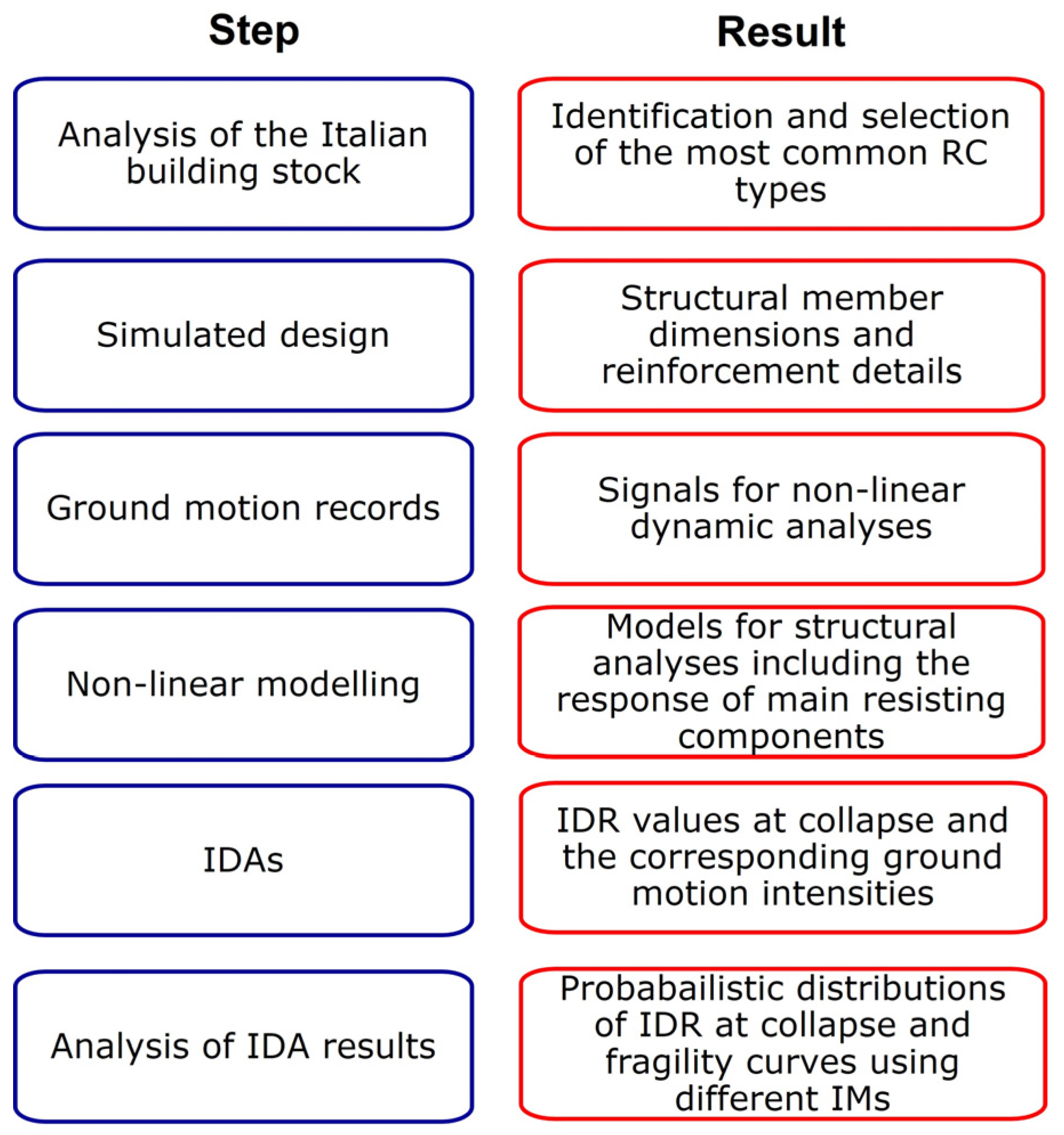
Assessing structural response at collapse is a delicate task, still a subject of active research. As reported in [1], it requires identifying several key aspects, such as possible modes of collapse, appropriate structural modeling of all main building components (structural and non-structural), ground motion selection, and the relevant epistemic and aleatory uncertainties.

Several studies have focused on these aspects. In the framework of non-linear dynamic response of structures, Ibarra and Krawinkler [21] studied the effect of stiffness and strength degradation by proposing a deteriorating hysteretic model that better represents the cyclic behavior of the structural members under large inelastic deformations, as observed in experimental tests. Based on the analyses carried out on several single-bay frames with varying number of storeys, they found that deterioration is of paramount importance in seismic collapse.

Haselton and Deierlein [18] focused on the role of modeling uncertainties, highlighting the influence of plastic rotation capacity as one of the main parameters affecting the seismic performance at collapse. Similarly, Goulte et al. [22] included both modeling uncertainties and spectral shape in the estimation of the collapse probability of a four-storey frame designed according to the 2003 International Building Code. Spectral shape was also investigated by Haselton and Baker [23] using single-degree-of-freedom models subjected to 70 ground motions. They found that the use of a more appropriate ground motion intensity measure (e.g., the spectral acceleration at a period approximately twice the fundamental period of the building) can reduce the sensitivity of collapse capacity estimates.

The key role of ground motion selection was also studied by Zhou et al. [24] through non-linear dynamic analyses of a modern 2D 6-storey Moment Resisting Frame (MRF). They found that ground motion selection plays a more significant role than modeling considerations on the predicted collapse probabilities and collapse risk. In the framework of ground motion selection, ten to twenty records are usually found to provide sufficient accuracy in the estimation of seismic demands, assuming a relatively efficient intensity measure is used (e.g., [25,26]).

Regarding the non-structural components to be used in seismic analyses, Sattar and Liel [27] focused on the role of infill in seismic collapse considering 2D frames representative of 1920s-era construction in Los Angeles. They pointed out that the presence of infill walls has a significant impact on the seismic response of a RC frame building, increasing strength, stiffness, and energy dissipation (relative to a bare frame), but simultaneously introducing brittle failure mechanisms associated with wall failure and wall-frame interaction.

Several studies were also carried out worldwide to assess the seismic collapse of building types using different analysis methods. In the framework of the RINTC project [28], which aims at estimating the annual failure rates of existing buildings designed according to the main Italian codes over time, Ricci et al. [14] studied the capacity at the Global collapse limit state of several code-conforming Italian RC building types by using non-linear static analyses. Roof drift ratio (RDR) values at collapse were identified along the post-peak softening branch corresponding to the 50% drop in base shear. They also emphasized the key role of infills: on the one hand, they significantly increase the base shear but, on the other hand, they fail in a brittle manner, leading to a sudden large drop in base shear, and thus resulting in a lower top displacement capacity compared to the corresponding bare types (i.e., in which infills were neglected). The same criterion was adopted by Pavel [29] for collapse assessment of some code-conforming RC frames in Romania.

Similarly, Di Domenico et al. [30] assessed the sidesway collapse capacity of some existing Italian RC buildings; the drop in base shear was evaluated by considering only the primary RC members, i.e., the infill contribution was excluded from the drop in base shear calculation.

The incremental non-linear dynamic analysis (IDA) method was adopted by Haselton et al. [18], who studied the collapse safety of twelve modern RC moment frames designed according to the governing provisions of the 2003 IBC, ASCE7-02 and the ACI 318-02. Similar analyses were also carried out by Mehrdad Shokrabadi et al. [31], who estimated the annual collapse risk for 30 modern, code-conforming RC moment frames without infills, designed based on the ASCE 7-05 and ACI 318-05.

Liel et al. [19] analyzed the seismic response at collapse of twelve non-ductile RC moment frames, varying in height from 2 to 12 storeys, representative of those built before the mid-1970s in California through IDAs performed with 80 signals. In modeling, special attention was paid to nonlinearities in beams, columns, beam-column joint and large P-Δ effects but the contribution of infills was not considered.

Noh and Tesfamariam [32] investigated the collapse risk assessment of code-conforming 2D RC MRF designed according to 2014 Canadian Building Code through IDAs, by varying the level of design (i.e., ductile and moderately ductile).

A comprehensive review of the analytical methods available to assess the capacity at collapse of buildings, which highlights the limitations of these methods and identifies what is required to accurately assess the seismic collapse capacity of a structure, is reported in [1]. The paper pointed out that methods based on non-linear static analyses may underestimate storey drift as certain aspects, such as cyclic effects, are neglected. Regarding IDA, the paper calls attention to some possible drawbacks related to the response-intensity curves, such as their nonmonotonic behavior, discontinuities, multiple collapse capacities, and variability from ground motion to ground motion, along with a high computational demand. However, these limitations can be mitigated by using larger set of signals and more efficient intensity measures able to reduce dispersion.

3. Methodology

According to the flowchart in Figure 1, the Italian building stock has been analyzed in the following sections to identify and select some of the most widespread RC types. The section dimensions and reinforcement details of these types have been obtained through the simulated design using the codes in force in the 1970s. After that, non-linear modeling has been defined to carry out incremental non-linear dynamic analyses (IDAs) using a set of real signals. Finally, the IDA results have been analyzed to estimate the probability distribution of inter-storey drift ratio values and the fragility curves at collapse in terms of different intensity measures.

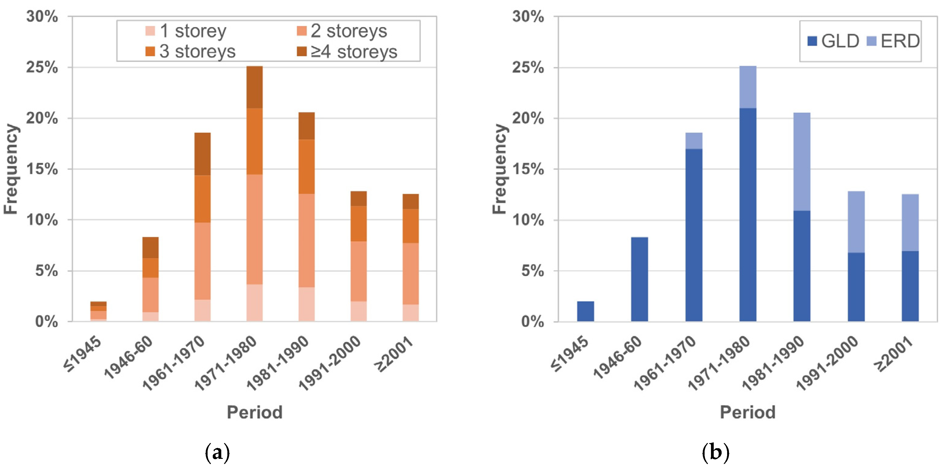
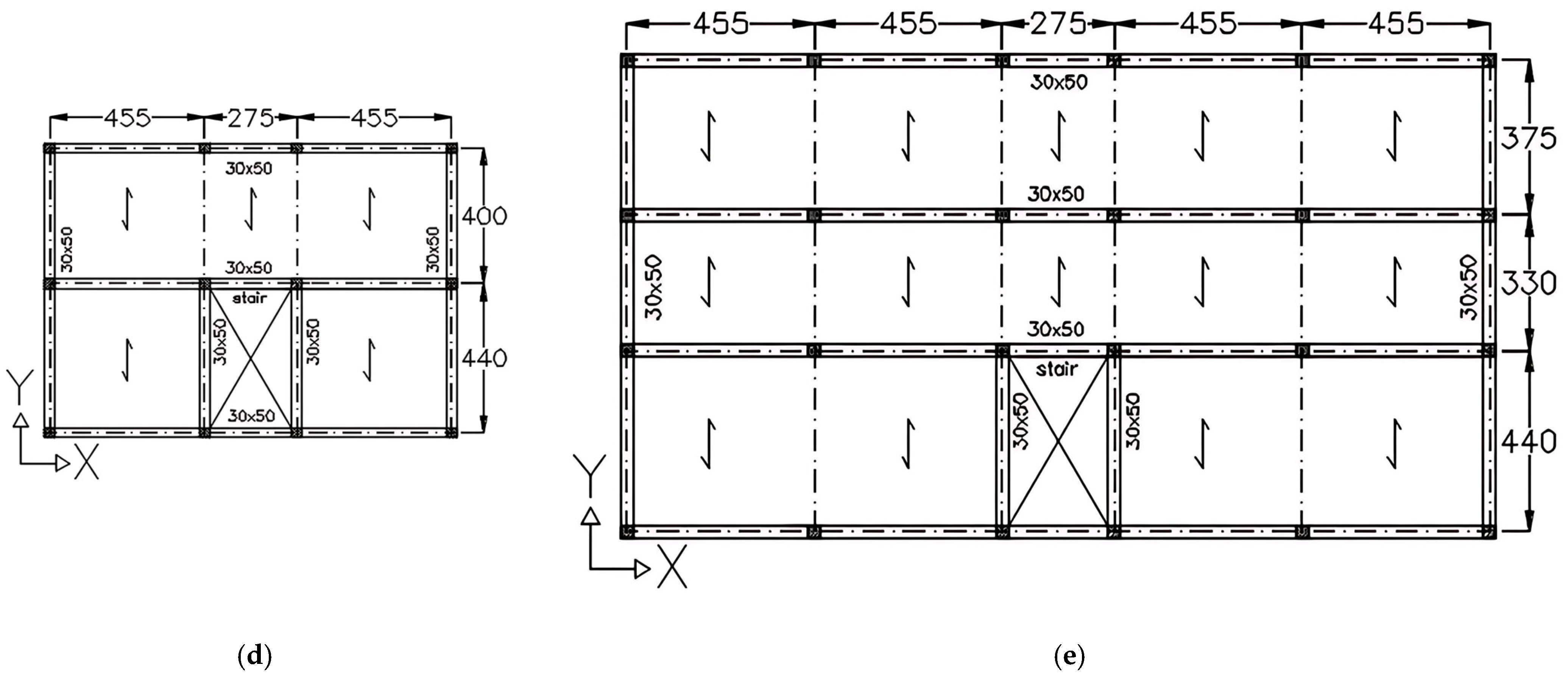
3.1. Selection of Building Types

Analyses at collapse have involved some building prototypes representative of the existing Italian RC building stock. The consistency of the Italian building stock was extensively analyzed in previous studies [33,34,35]. According to the ISTAT 2011 Census of Population and Houses [36], the Italian building stock amounts to about 12 million buildings, of which about 7 million are masonry structures mainly built before the end of World War II, whereas reinforced concrete (RC) buildings (about 4 million) became the main structural type starting from the 1950s.

Specifically for RC buildings, Figure 2 shows the distribution of the Italian RC building stock in terms of the number of storeys (Figure 2a). Most of the RC building stock was built in the period 1961–90, with a prevalence (about 25%) in the 1970s. The same figure also shows that most RC buildings have 1–2 storeys in elevation (i.e., low-rise types, 58%) while the remaining 42% consists of buildings with 3 or 4+ storeys (i.e., mid-rise types also including high-rise ones). Note that the considered database does not provide information on buildings with 6 or more storeys (i.e., high-rise types). However, other studies based on more refined data for specific towns (e.g., [35]) reveal a significant relative percentage (up to 25%) of high-rise building types.

In terms of design level, Figure 2b shows that about 73% of buildings was designed only for gravity loads. On the contrary, starting from the 1970s, an increasing percentage of buildings was seismically designed (about 15%), although adopting low lateral forces without any seismic details.

Design rules for RC buildings can be categorized into two major periods: before 1971 and after 1971. Indeed, in 1971, Law 1086 [37] and Law 64/1974 [38] implemented important administrative procedures related to both design and construction phases that generally ensured higher construction quality. For example, they established a systematic procedure to check the adopted material strength and formalized the role of a dedicated technician to verify the entire construction process. Furthermore, they permitted the use of stronger materials in design practices. Specifically, before 1971, Royal Decree 2229/1939 [39] considered three types of steel quality, i.e., low-carbon, medium-carbon and high-carbon steel, whose nominal tensile stress values at yielding are in the range of 230–310 MPa. Note that only smooth bars were produced during that period. In the 1970s, due to a more flexible code-upgrading process permitted by Law 1086/1971, several ministerial decrees were issued, addressing to the use of material with increasing strength. Deformed steel bars were introduced with yield stress values ranging from 380 to 440 MPa.

As for seismic design, Law 25/11/1962 [40] introduced the distribution of seismic forces as a function of the lateral stiffness of frames. Before that, according to Royal Decree 640/1935 [41], lateral forces had to be applied to each single plane frame based on the gravity loads (dead and live loads) acting on it, implicitly neglecting the in-plane redistribution due to RC slabs. Until OPCM 3274/2003 [42], which classified the entire Italian territory as seismic and introduced modern anti-seismic criteria for both new constructions and the assessment/retrofit of existing buildings according to international standards, there were no significant differences in design criteria compared to gravity load design. The main distinctions were in the lateral load distributions applied to structures (i.e., uniform and inverted triangular) and their intensities, which were 7% or 10% of the “seismic weight” (i.e., dead loads and a portion of the live loads, typically equal to 1/3) for categories I and II, respectively.

As for infills, the types mainly adopted changed over time due to the energy demand reduction requirements introduced by codes [43]. In the 1950s, infills typically consisted of a single layer of solid bricks (25 cm thick) or two layers (comprising solid or hollow clay bricks) with an empty cavity. This type was also common in the 1970s, featuring an external layer (12 cm thick), an internal layer (8 cm thick), and an empty cavity (10 cm thick), for a total thickness of 30 cm. In the 1990s, the two layers of hollow bricks were thicker, especially the external layer (15–20 cm thick).

Taking into account the most common Italian building types (Figure 2), prototypes with 2-, 4-, and 6-storeys (hereafter 2s, 4s, and 6s, respectively) have been selected to represent low-, mid-, and high-rise building types designed according to the codes in force in the 1970s by considering either only gravity loads (hereafter GLD) or low lateral forces (II category, hereafter ERD), consistent with pre-code and low-code types, respectively.

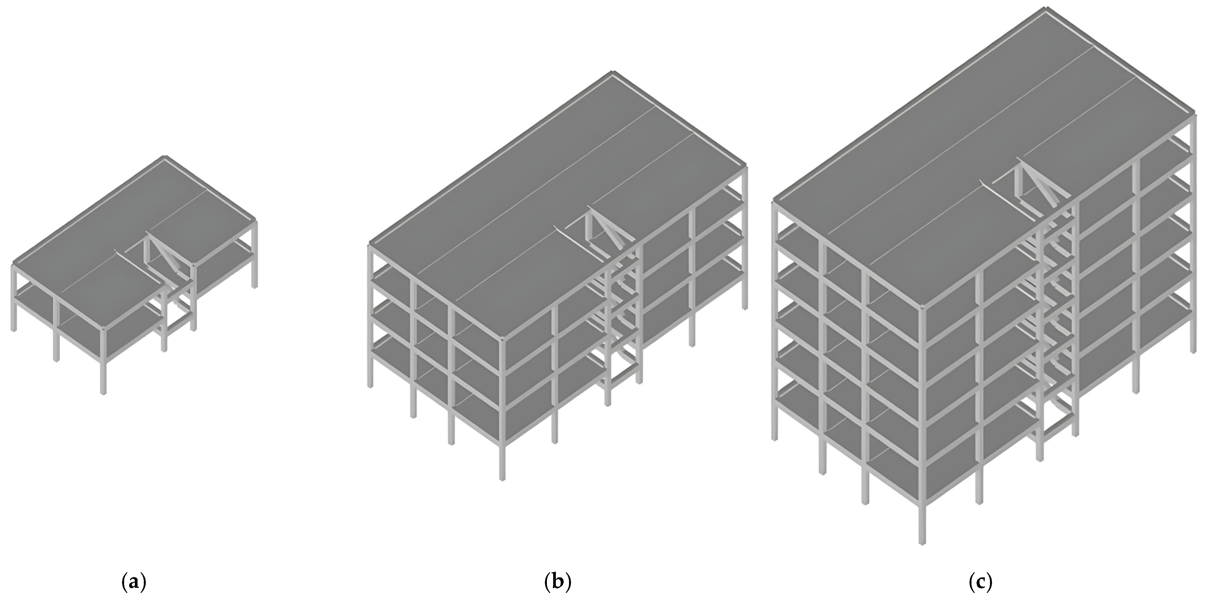
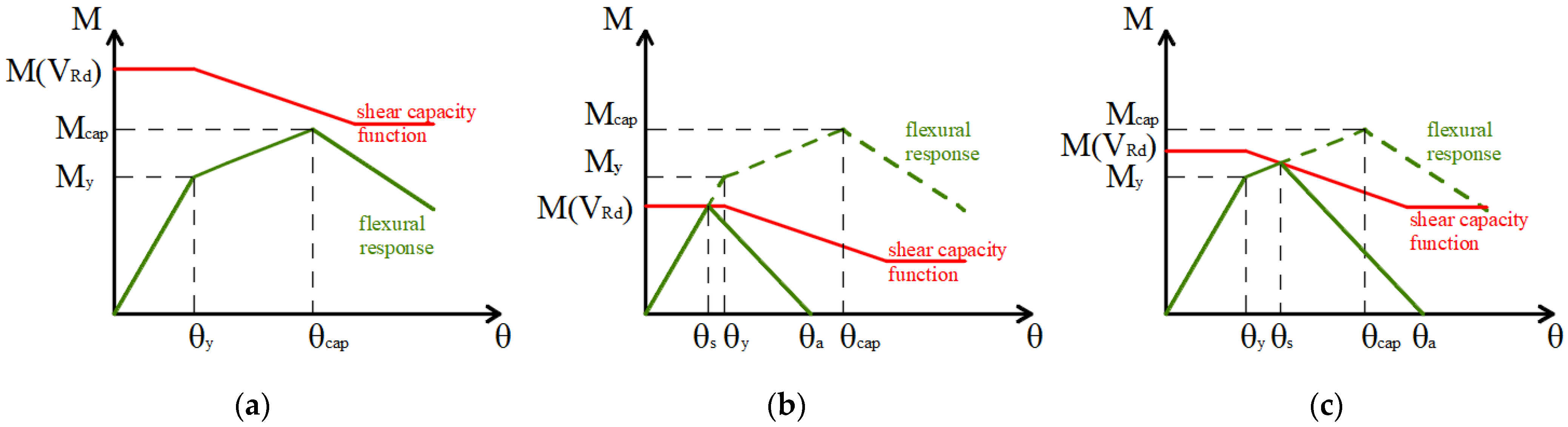
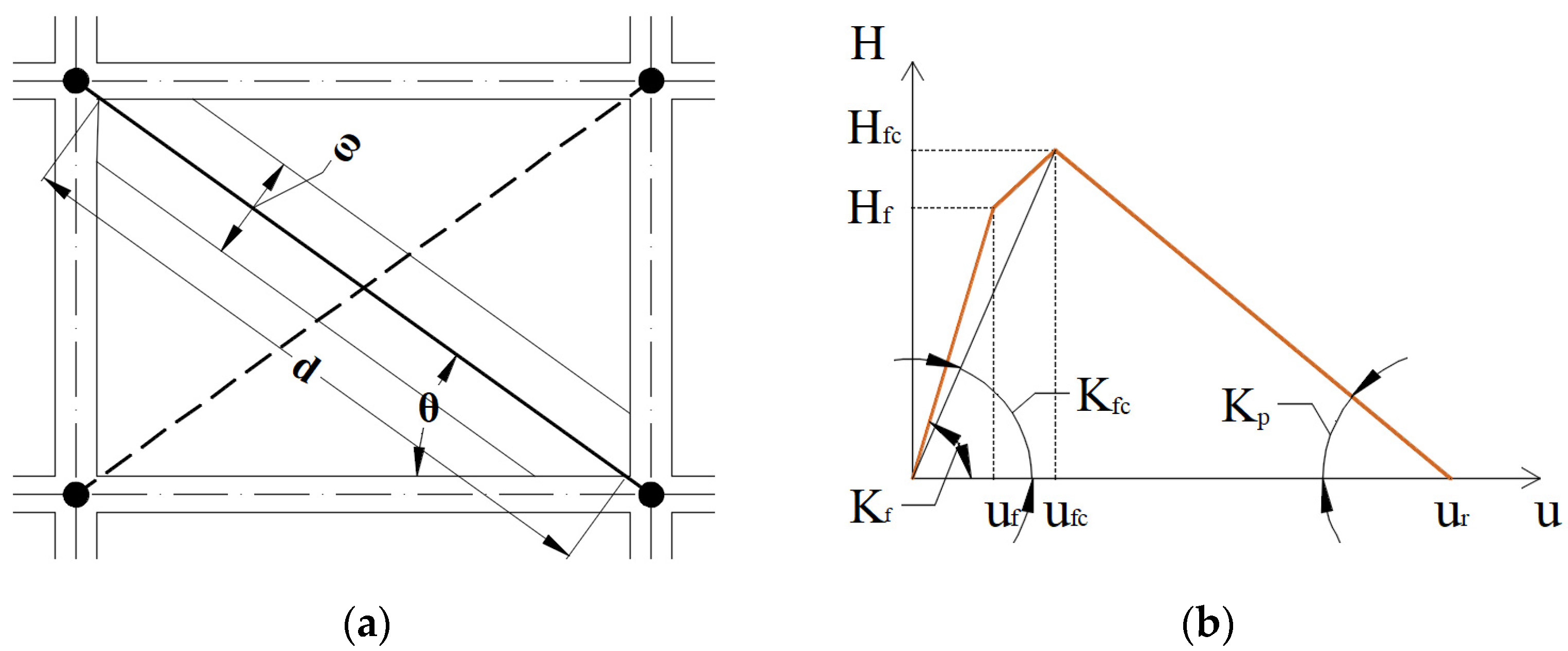
3.2. Design and Modeling

All building types have a rectangular in-plane shape (Figure 3) with different dimensions and numbers of bays along the two orthogonal directions. Specifically, 2s types have overall dimensions of 12.15 × 8.70 m², featuring three bays along the X direction and two bays along the Y direction. On the other hand, both 4s and 6s buildings have overall dimensions of 20.95 × 11.75 m², with five bays along the X direction and three bays along the Y direction. All prototypes have a uniform inter-storey height equal to 3.05 m.

In line with the common practice of the 1970s, the lateral resisting scheme comprises plane frames with rigid beams only along the X direction. Along the Y transverse direction, beams are present only in the exterior frames. The staircase sub-structure is symmetrically positioned with respect to the Y direction and includes knee-type beams.

As for infills, a double-layer configuration with hollow clay bricks and an empty cavity has been considered for all prototypes. The external and internal layers are 12 cm and 8 cm thick, respectively. The infills placed in the exterior frames along the Y direction have no openings, whereas the opening percentages of the infills along the X direction are in the range of 25–45%.

For each prototype, cross-section dimensions and reinforcement details have been determined using the simulated design [44], considering the codes in force in that period, common design practices, and typical material properties. Specifically, the Ministerial Decree of 30 May 1972 [45] has been considered for GLD types (i.e., types designed only for gravity loads), while Law 1684/1962 [40] was applied to ERD types (i.e., types designed with low lateral force without anti-seismic details). Note that Law 1684/1962 does not provide any anti-seismic prescriptions (e.g., transverse reinforcement in beam-column joints) while, for the 2nd seismic category, it sets the lateral forces to be applied at 7% of the “seismic weight” (i.e., dead loads and 1/3 of the live loads), with a constant distribution along the height. Internal forces have been determined using simplified models that, in the case of GLD types, resulted in continuous beams resting on simple supports and columns subjected to only axial loads according to the tributary area. As for ERD, seismic actions have been distributed among the plane frames based on their respective lateral stiffness.

For both GLD and ERD types, typical mechanical properties as a function of the period have been assumed from the literature. More specifically, concrete with a nominal compressive strength of 25 MPa and deformed bars with a nominal tensile yield strength of 380 MPa has been considered.

The large number of analyses has required pragmatic modeling choices. Specifically, to ensure both robustness and a reasonable computation demand, a lumped plasticity approach, along with the phenomenological response of hinges, has been adopted within the OpenSees package [46], following the main criteria defined by De Risi et al. [33] and Di Domenico et al. [30] in the RINTC project [28].

This approach effectively describes the post-peak degrading response, which is one of the most important aspects affecting the collapse of structures, along with cyclic deterioration effects, as reported in the Literature review (Section 2).

For this purpose, the flexural response of each hinge, expressed in terms of the moment–rotation relationship (M-θ), has been modeled according to the trilinear Ibarra–Medina–Krawinkler (IMK) model [21], which is able to take into account all the most important modes of deterioration observed in experimental tests under large inelastic deformations, including the effects of stiffness and strength degradation. The model, which consists of seven parameters, has been widely used in analyses of collapse for both existing and code-conforming structures (e.g., [19]).

The backbone parameters of the IMK model have been evaluated using the predictive equations by Haselton et al. [47], which were obtained by statistical regression on a large experimental database of RC members with deformed bars.

Unlike the fibre-based approach, which accounts for the interaction between the planes of flexure and axial load, in the adopted modeling approach, an independent M–θ relationship has been defined for each plane of flexure under a constant axial load. On the contrary, the phenomenological model allows to easily modify its response to account for shear effects. Specifically, in the case of brittle failure (e.g., the short columns of the staircase structure), the M–θ relationship has been modified to account for shear degradation as a function of ductility demand, following the Sezen and Moehle model [48]. Three cases emerge from the comparison between the flexural response and the corresponding shear capacity function: (i) flexural mode, where the column fails in flexure; (ii) shear mode, where the column fails in shear before reaching the yielding moment; and (iii) an intermediate condition (shear/flexural mode), where the column fails in flexure due to a bending moment within the yielding to capping range, as shown in Figure 4.

As for infill modeling, an equivalent single-strut approach (Figure 5a) has been adopted, with the cross-sectional area calculated by multiplying the panel thickness by an equivalent width, ω, evaluated according to the Decanini and Fantin model [49], as follows:

$$\omega =\left({\displaystyle \frac{K_1}{\lambda h}}+K_2\right)d$$

(1)

where λh is a non-dimensional parameter that depends on the geometric and mechanical characteristics of the frame-infill system, K₁ and K₂ are coefficients that change according to λh, and d is the length of the equivalent strut, as shown in Figure 5a.

The in-plane response of struts has been modeled based on the trilinear backbone model adopted by Ricci et al. ([14,50]), as reported in Figure 5b. The first linear elastic ascending branch corresponds to the un-cracked stage, and the second branch refers to the post-cracking phase up to the development of the maximum strength (H_fc). The descending third branch of the curve describes the post-peak strength deterioration of the infill until it reaches the residual (zero) strength at displacement u_r. The characteristic points of the in-plane response (Figure 5b) have been evaluated as follows:

$$K_{fc}={\displaystyle \frac{E_{wall}e\omega }{d}}co{s}^2\theta$$

(2)

$$K_p=-0.02K_{fc}$$

(3)

$$H_{fc}=f_{c,wall}e\omega cos\theta$$

(4)

$$H_f=0.8H_{fc}$$

(5)

where f_c,wall and E_wall are the compressive strength and the elastic modulus of infills and θ is the inclination of the diagonal strut. Further details can be found in Ricci et al. ([14,50]).

Considering the typical mechanical properties of materials used in buildings from the specified period ([51,52]), a mean concrete strength value (f_cm) of 20 MPa and a mean steel strength value (f_ym) of 400 MPa have been assumed for evaluating structural capacity. Based on literature values for the infill type ([43,53]), the compressive strength is assumed to be 1.2 MPa, with an elastic modulus of 2000 MPa.

Table 1. Main mechanical parameters considered in modeling, averaged over all columns of the first storey. The last column shows the fundamental period values of vibration (T1).

Type	ρl_X [%]	ρl_Y [%]	ρw_Y [%]	ρw_Y [%]	Mcap_X [kNm]	Mcap_Y [kNm]	θcap_X [-]	θcap_Y [-]	T1 [s]
2s-GLD	0.28	0.28	0.11	0.11	68.2	68.2	0.0235	0.0245	0.25
4s-GLD	0.25	0.29	0.11	0.10	101.2	88.3	0.0181	0.0131	0.49
6s-GLD	0.24	0.31	0.10	0.08	145.1	117.0	0.0106	0.0100	0.77
2s-ERD	0.50	0.31	0.09	0.09	114.3	102.2	0.0113	0.0135	0.23
4s-ERD	0.56	0.30	0.10	0.08	216.4	108.4	0.0165	0.0121	0.49
6s-ERD	0.53	0.27	0.07	0.07	320.3	195.2	0.0082	0.0082	0.70

Note: ρ_l_X/Y is the tension reinforcement ratio, defined as the ratio of the cross-sectional area of tensile reinforcement to the product of the compression zone width and the effective depth of the cross-section; ρ_w_X/Y is the transverse reinforcement ratio, defined as the ratio of the total cross-sectional area of the transverse reinforcement to the product of the transverse reinforcement spacing and the cross-section width; M_cap_X/Y and θ_cap_X/Y are the plastic moment and rotation at capping, respectively, evaluated according to the trilinear Ibarra–Medina–Krawinkler (IMK) model [21]. Each parameter is an average value calculated for all the columns of the first storey along the X and Y directions.

shows the main mechanical parameters considered in modeling and the fundamental period values of vibration for all the considered types.

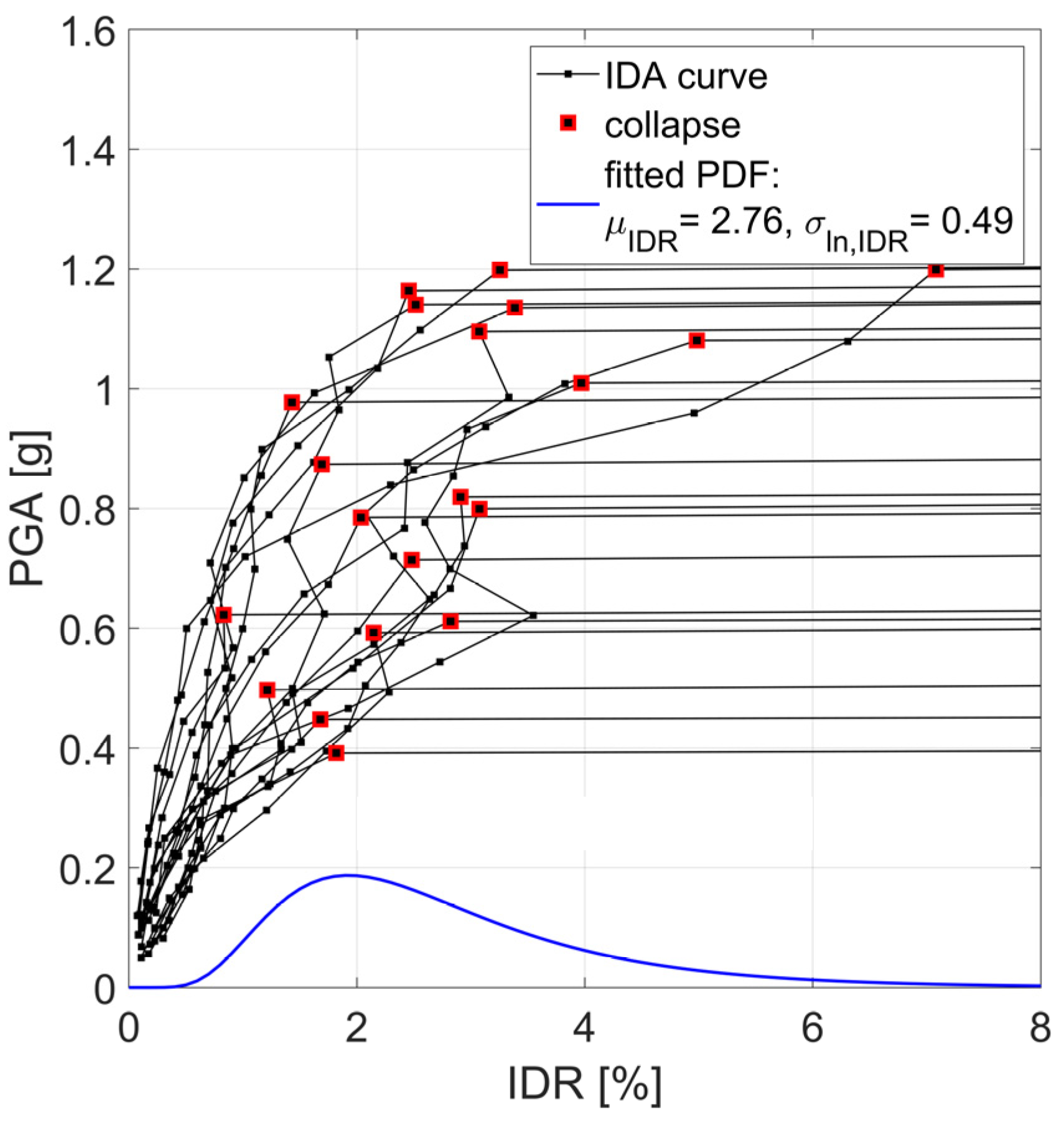
3.3. Incremental Dynamic Analyses

Keeping in mind the intrinsic advantages and limitations in performing IDA as reported in Section 2, in order to analyze the structural response at collapse, the Incremental non-linear Dynamic Analysis (IDA, [15]) method has been adopted. Although many analysis methods exist in the literature (e.g., [54,55]), IDA is one of the most powerful methods widely used by researchers for simulating structural response through non-linear dynamic analyses, able to account for record-to-record variability. For a given suite of records, IDA consists of performing non-linear dynamic analyses by monotonically scaling the considered dataset of signals until dynamic instability is reached, i.e., when deformations increase indefinitely with small increments of the considered intensity measure. In doing so, some drawbacks may arise due to excessive scaling (e.g., [16]), especially when a poor efficient intensity measure is considered, as the selected records at any given ground motion intensity level should ideally reflect the expected dominant ground motion characteristics [20]. Zacharenaki et al. [56], on a variety of structures, ranging from stiff to flexible, showed that for small periods, i.e., lower than 0.5 s, there is a significant bias, and the IDA method tends to underestimate the response, while the bias diminishes considerably as the period increases.

To adequately account for record-to-record variability, it is essential to consider a sufficient number of records. For this purpose, some studies suggest using 20–30 records [57], to ensure adequate variability while maintaining manageable computational demand.

In this paper, IDAs have been performed using a dataset of 20 real signals consistent with the Italian hazard characteristics, extracted from a large database of recorded signals, SIMBAD [58], using the S&M tool [59]. In S&M, signals are selected by approaching a user-defined target spectrum in a broad period range, with weighted selection parameters. In this study, the 5%-damped elastic design spectrum defined for L’Aquila city (design ground acceleration on rock, a_g = 0.261 g) according to the current Italian code [60] has been considered. Furthermore, magnitude values have been constrained to be lower than Mw 7 and soil conditions A/B (i.e., stiff soil, average shear wave velocity in the top 30 m, V_S30 > 360 m/s, according to the current Italian code [60]). As reported in

Table A1. Main parameters of the considered dataset of signals.

Signal	Mw	Repi [km]	VS30 [m/s]	PGA [g]	PGV [cm/s]	HI [m]	Sa (T1 = 0.25 s) [g]	Sa (T1 = 0.5 s) [g]	Sa (T1 = 0.75 s) [g]	Sa,avg [g]	AI [m/s]
#1	6.4	21.37	na	0.11	6.12	0.26	0.37	0.16	0.11	0.06	0.14
#2	5.7	18.73	408	0.12	8.44	0.23	0.32	0.10	0.05	0.06	0.08
#3	5.6	5.9	378	0.13	10.40	0.29	0.28	0.21	0.12	0.07	0.12
#4	5.9	27.77	363	0.10	4.46	0.22	0.12	0.08	0.07	0.05	0.11
#5	6.9	23.77	1149	0.06	5.06	0.20	0.13	0.11	0.06	0.05	0.06
#6	6	17.53	na	0.12	9.60	0.29	0.26	0.18	0.11	0.07	0.10
#7	5.6	10.33	626	0.14	6.65	0.22	0.30	0.19	0.08	0.05	0.10
#8	5.6	9.35	717	0.08	4.74	0.20	0.20	0.13	0.07	0.05	0.07
#9	5.5	15.81	452	0.09	5.60	0.17	0.27	0.09	0.05	0.04	0.07
#10	6.5	20.1	na	0.09	5.84	0.17	0.08	0.07	0.05	0.04	0.09
#11	6.4	20.83	852	0.10	9.09	0.28	0.21	0.27	0.12	0.07	0.09
#12	5.4	16.16	717	0.05	4.14	0.19	0.07	0.07	0.07	0.04	0.02
#13	6.4	30	na	0.12	8.39	0.32	0.33	0.21	0.08	0.08	0.14
#14	5.7	25.39	409	0.07	4.42	0.16	0.13	0.13	0.08	0.04	0.04
#15	5.9	10.04	901	0.13	6.34	0.18	0.27	0.11	0.11	0.04	0.16
#16	5.6	25.24	412	0.12	4.20	0.19	0.31	0.06	0.05	0.05	0.08
#17	6.1	29.53	403	0.11	4.24	0.16	0.24	0.10	0.11	0.04	0.14
#18	5	7.84	529	0.10	5.54	0.17	0.23	0.15	0.08	0.04	0.05
#19	5.9	23.85	601	0.08	6.73	0.16	0.13	0.13	0.09	0.04	0.05
#20	5.4	12.29	685	0.07	5.17	0.17	0.13	0.12	0.10	0.04	0.03

Note: Mw = moment magnitude; R_epi = epicentral distance; V_S30 = average shear wave velocity in the top 30 m; PGA = Peak Ground Acceleration; PGV = Peak Ground Velocity; HI = Housner intensity; Sa(T1) = pseudo-spectral acceleration evaluated at the fundamental period of vibration equal to 0.25 s, 0.50 s, and 0.75 s; Sa,avg = average spectral acceleration; AI = Arias intensity; na = not available.

(Appendix A), the selected records have magnitude values ranging from 5.0 to 6.9, epicentral distances R_epi between 5.9 and 30 km, and V_S30, between 363 and 540 m/s.

From each IDA, the maximum inter-storey drift ratio value (IDR), assumed as Earthquake Demand Parameter (EDP), reached at collapse along with the corresponding Intensity Measure (IM) value have been collected. The IM values include the most commonly used measures in earthquake engineering, such as Peak Ground Acceleration (PGA), Peak Ground Velocity (PGV), Housner intensity (HI), pseudo-spectral acceleration at the fundamental period of vibration Sa(T1) evaluated for each type (see Table 1), average spectral acceleration (Sa,avg) [61] and Arias intensity (AI).

As better explain in Section 4.1 and Section 4.2, the dataset of EDP values at the onset of collapse has been processed to estimate the IDR values for the considered types. A lognormal probability density function has been fitted to the data, and the mean and 16th and 84th percentiles have been estimated. Fragility curves at collapse have also been derived by fitting the fractions of records causing collapse at each IM value. For this purpose, a lognormal cumulative distribution function has been adopted in order to provide a continuous estimate of collapse probability as a function of IM.

4. Results

The methodology described above has been used to obtain IDA curves for all types. Figure 6 shows the median IDA curves in terms of PGA for 2s (Figure 6a), 4s (Figure 6b) and 6s (Figure 6c) types along the X and Y directions, by varying the design level (i.e., gravity load design, GLD, and earthquake resistant design with low lateral force intensity without anti-seismic details, ERD). For ERD types, the PGA values corresponding to almost all IDR values are generally higher than those for GLD, as expected, with larger differences observed at collapse (i.e., flatline) for 4s and 6s types. Two different trends are found for the IDA curves along the two in-plane directions. In the case of GLD, the X direction exhibits lower PGA values compared to the Y direction, whereas the opposite is observed for the ERD types. Since both GLD and ERD structures have the same lateral resisting scheme (see Figure 3) the higher lateral capacity observed for GLD in the Y direction is due to the staircase substructure and infill walls (which have no openings). On the contrary, lateral loads in ERD types increase the lateral capacity of the frames along the X direction more than those along the Y direction. For this purpose, it is worth noting that along the X direction there are a greater number of frames compared to the frames along the Y direction, which are placed only on the exterior sides. Furthermore, in the Y direction, a greater number of brittle failures have been detected in the columns’ response of ERD compared to both the X direction and the Y direction of GLD.

In the following sections, the results from IDA are further processed in order to determine the IDR distribution values at collapse (Section 3.1) and to derive fragility curves using different IMs (Section 3.2). Both results are compared in order to highlight the role of the considered typological parameters on collapse response.

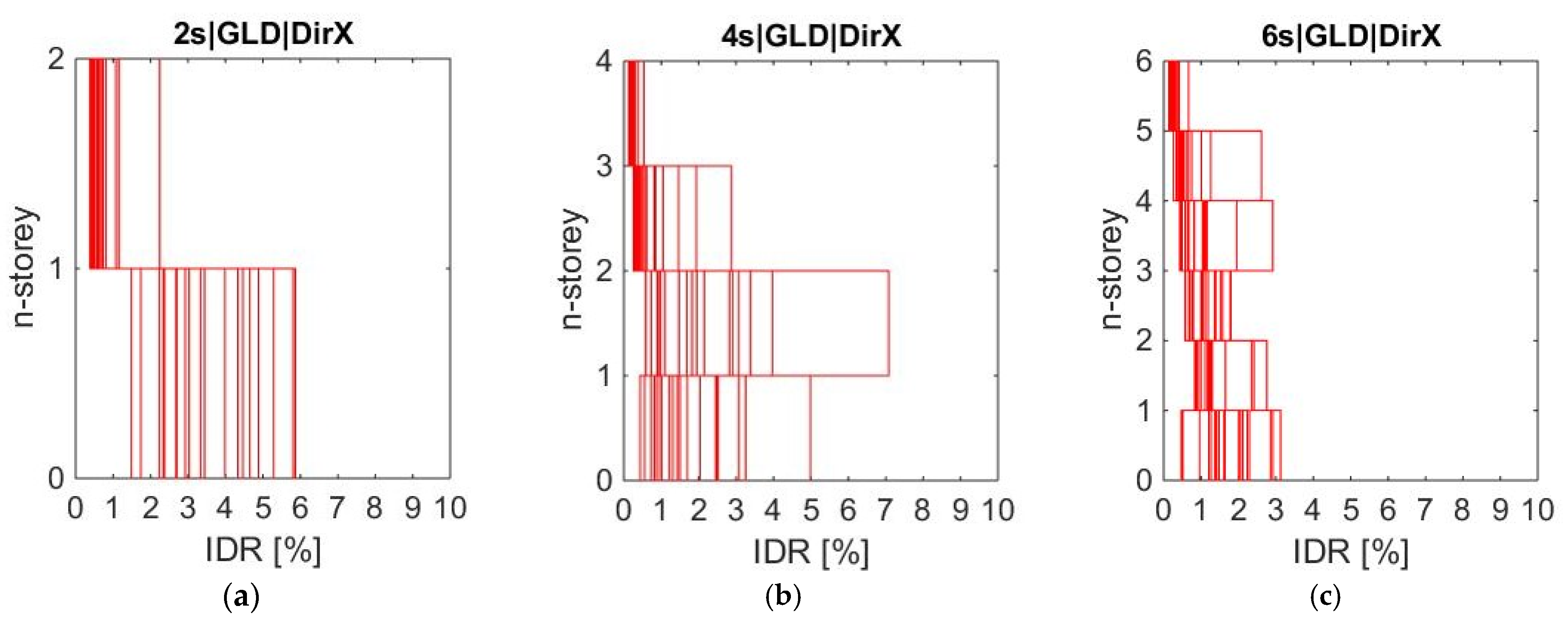
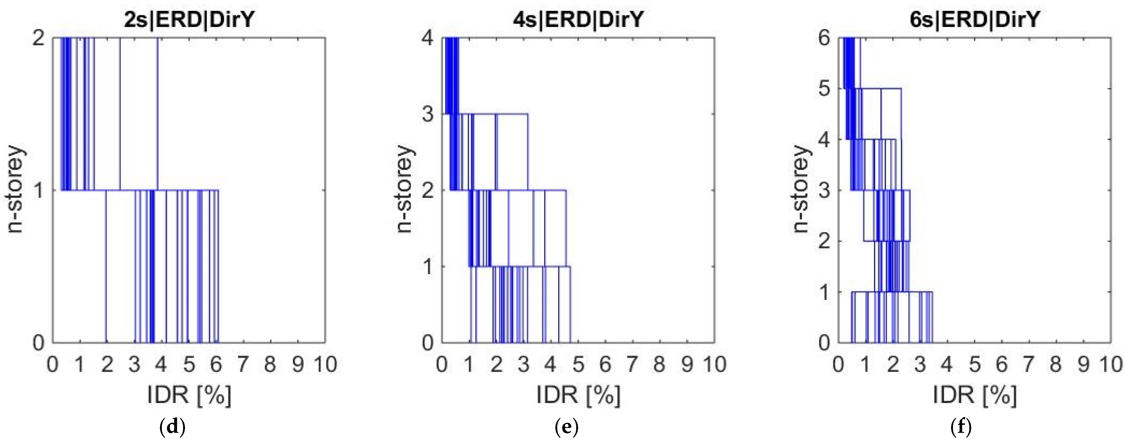
4.1. Inter-Storey Drift Ratio at Collapse

The IDR results at collapse obtained from IDAs for each considered type have been collected and fitted according to a lognormal distribution, whose equation is as follows:

$$f\left(x\right)={\displaystyle \frac{1}{\sqrt{2\pi }\left({\sigma }_{ln}x\right)}}{e}^{-{\displaystyle \frac{1}{2}}({\displaystyle \frac{lnx-\mu }{{\sigma }_{ln}}}{)}^2}$$

(6)

where x is the IDR variable, µ and σ_ln are the mean and lognormal standard deviation of the distribution. These two parameters have been obtained by fitting each set of IDR data using common computational software programs (e.g., Matlab R2024b, https://it.mathworks.com/products/matlab.html, accessed on 7 April 2025).

As an example, Figure 7 shows the results obtained from the IDAs performed for the 4s-GLD type along the X direction in terms of PGA. In the plot, the dynamic instability is graphically represented by the flatline, and the point where the flatline begins indicates the IDR value at collapse (black squares with a red marker edge in Figure 7). Figure 7 also shows the fitted lognormal probability density function (blue line in Figure 7), along with µ_IDR and σ_ln,IDR values.

Table 2. Mean values (with the 16th- and 84th-percentiles) and lognormal standard deviations of the lognormal distribution of IDR values along the X- and Y-directions for all types. The minimum values between the in-plane directions are highlighted in bold.

		GLD			ERD
		2s	4s	6s	2s	4s	6s
IDR dirX	µ (16th–84th) [%]	3.52 (2.19–4.82)	2.76 (1.50–3.99)	1.93 (1.28–2.57)	7.38 (5.02–9.72)	5.37 (2.87–7.80)	6.31 (3.18–9.33)
	σln	0.40	0.49	0.35	0.33	0.50	0.54
IDR dirY	µ (16th–84th) [%]	4.81 (3.03–6.57)	3.56 (2.29–4.82)	2.53 (1.82–3.24)	4.43 (3.22–5.64)	2.89 (1.93–3.84)	2.40 (1.87–2.93)
	σln	0.39	0.37	0.29	0.28	0.35	0.22

shows the main statistical parameters of Equation (6) (i.e., µ and σ_ln), along with the 16th and 84th percentile values, estimated for both in-plane directions of each type.

From these results, some general remarks can be made.

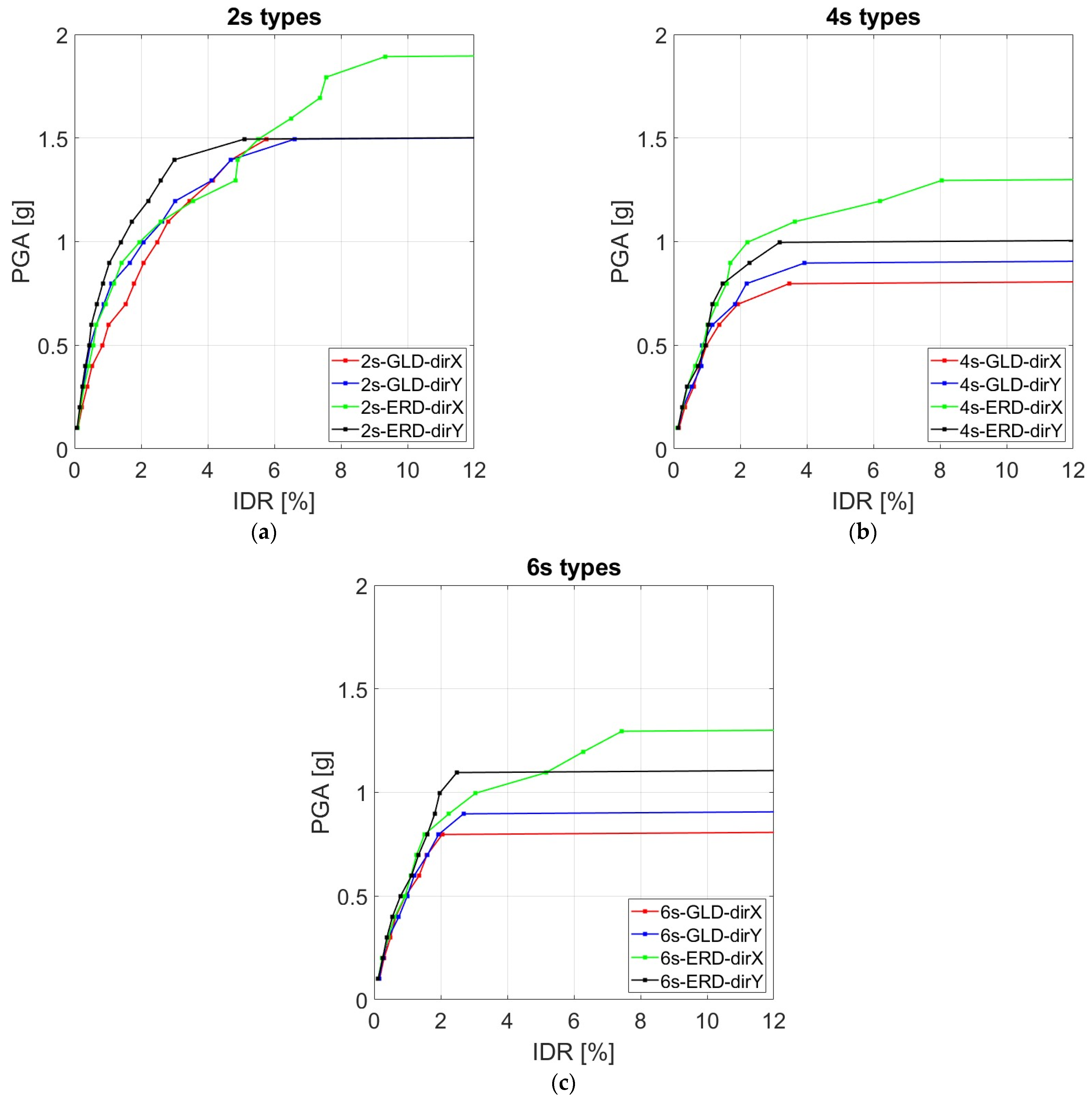
• IDR values decrease as the number of storeys increases for both GLD and ERD types. Specifically, the minimum mean values for GLD are approximately 3.5%, 2.8%, and 1.9% for 2s, 4s, and 6s types, respectively, while they become 4.4%, 2.9%, and 2.4% for ERD. To understand the observed trend, it is important to note that the collapse mechanism for each type generally involves the bottom storeys, as illustrated in Figure 8, which illustrates the IDR profiles related to the minimum values along the X and Y directions. Since cross-section dimensions of columns and the related reinforcement details do not change significantly across the storeys, the displacement capacity reduces with the number of storeys (i.e., as axial forces increase). This aspect can be better acknowledged in Table 1, where the plastic rotation values (at capping) for the columns of the first storey are reported for all types.
• The minimum IDR values among the two in-plane directions detected for ERD are higher compared to GLD types, with increments of about 25% for 2s and 6s and about 5% for 4s. A different trend is observed between the two in-plane directions. For GLD, the X direction exhibits lower IDR values compared to the Y direction, whereas the opposite is found for the ERD types, with notable differences between the X and Y directions. For this purpose, it is worth noting that, in GLD, the cross-section dimensions and reinforcements details of the columns are quite similar for both in-plane directions. Therefore, the greater lateral displacement capacity along the Y direction mainly depends on the contribution of stairs and infills (which have no openings along the Y direction). On the contrary, lateral forces considered for ERD types significantly increase the lateral displacement capacity of the frames along the X direction compared to those along the Y direction. Indeed, as previously described, the lateral resisting scheme of the considered prototypes has a greater number of frames along the X direction compared to those along the Y direction, which are placed only on the exterior sides. Furthermore, the columns’ response along the Y direction exhibits a greater number of brittle failures compared to the X direction. Finally, note that, according to the common practice of the period, the contribution of the staircase sub-structure is the same as in GLD, since it has been designed only for vertical loads.
• As for dispersion, the σln values associated with the minimum IDR range from 0.35 to 0.49 for GLD, while lower values (0.22–0.35) are observed for ERD. Although simple schemes have been adopted, the interior force analyses carried out for EDR types generally reduce the variability of the response at collapse with respect to GLD, whose structural members have mainly been designed by adopting the minimum requirements of codes.

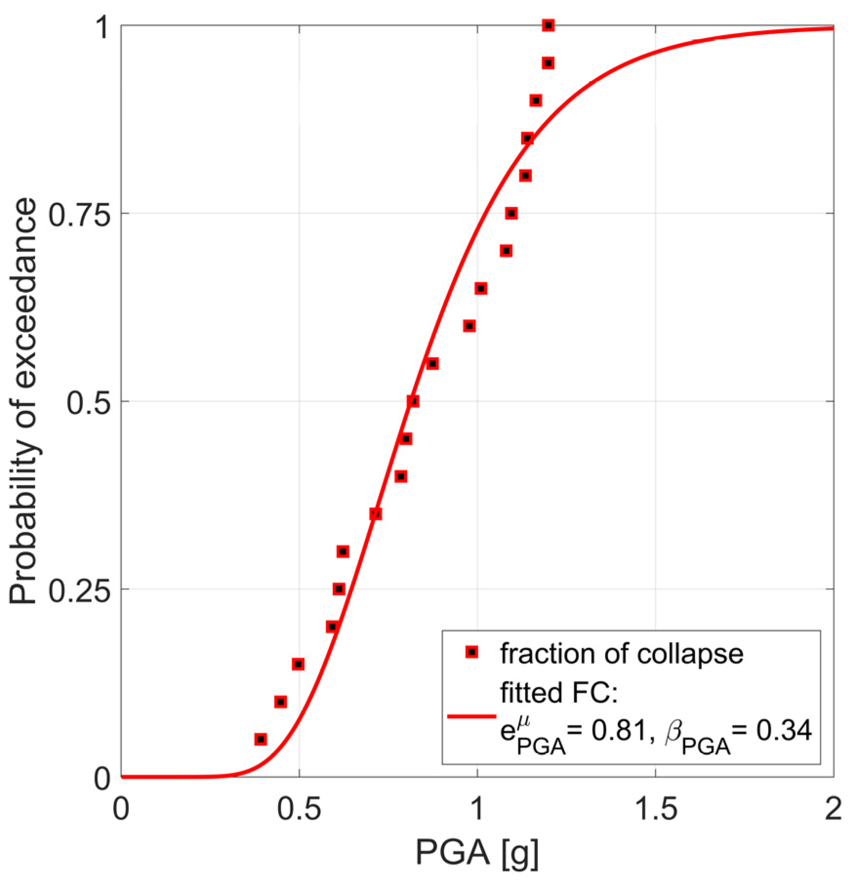
4.2. Fragility Curves at Collapse

The dataset of IDR values from has also been used to estimate the conditional probability of exceedance (i.e., Fragility Curve, FC) of collapse, as a function of the intensity measure (IM). For this purpose, the commonly adopted lognormal cumulative distribution function (CDF, [62]) has been used, as follows:

$$P(C|IM=x)=\mathsf{\Phi }\left[{\displaystyle \frac{\ln \left(\frac{x}{e^{\mu }}\right)}{\beta }}\right],$$

(7)

where $P(C|IM=x)$ is the probability of exceedance of collapse (C) given an IM value equal to x (IM = x), $\mathsf{\Phi }$ is the standard normal (Gaussian) cumulative distribution function, and β and $e^{\mu }$ denote the logarithmic standard deviation and median (i.e., 50% probability of not exceeding) values of IM related to collapse, respectively. The two parameters characterizing the CDF, i.e., β and $e^{\mu }$, have been calculated as reported in Appendix B, by using the common procedure provided by Baker [63].

As an example, Figure 9 shows the fragility curve derived for the 4s-GLD type along with the cumulative distribution of records causing collapse as obtained from IDAs.

Table 3. Median e^µ and lognormal standard deviation β related to the fragility curves derived for all types in terms of different IMs. The minimum values between the in-plane directions are highlighted in bold.

Type	In-Plane Direction	PGA		PGV		HI		Sa(T1)		Sa,avg		AI
		eµ [g]	β [-]	eµ [cm/s]	β [-]	eµ [m]	β [-]	eµ [g]	β [-]	eµ [g]	β [-]	eµ [m/s]	β [-]
2s-GLD	Dir-X	1.38	0.32	86.01	0.28	2.95	0.15	2.84	0.51	0.71	0.16	15.99	0.55
	Dir-Y	1.41	0.31	88.22	0.25	3.02	0.13	3.12	0.46	0.73	0.14	16.82	0.53
4s-GLD	Dir-X	0.81	0.34	50.86	0.31	1.74	0.20	1.04	0.73	0.42	0.20	5.59	0.53
	Dir-Y	0.93	0.35	57.99	0.32	1.99	0.24	1.02	0.69	0.48	0.23	7.27	0.60
6s-GLD	Dir-X	0.81	0.39	50.80	0.30	1.74	0.22	0.68	0.47	0.42	0.21	5.58	0.69
	Dir-Y	0.84	0.34	52.28	0.24	1.79	0.16	0.72	0.56	0.43	0.15	5.91	0.63
2s-ERD	Dir-X	1.69	0.28	105.7	0.21	3.62	0.11	3.49	0.46	0.87	0.12	24.18	0.49
	Dir-Y	1.45	0.29	90.39	0.26	3.10	0.18	3.20	0.47	0.74	0.19	17.66	0.53
4s-ERD	Dir-X	1.29	0.32	79.02	0.30	2.77	0.22	1.61	0.41	0.65	0.22	14.14	0.53
	Dir-Y	1.09	0.40	68.22	0.31	2.34	0.21	1.09	0.68	0.56	0.21	10.06	0.72
6s-ERD	Dir-X	1.26	0.38	80.87	0.34	2.71	0.21	1.08	0.43	0.67	0.23	13.50	0.63
	Dir-Y	0.98	0.34	61.46	0.31	2.10	0.20	0.94	0.56	0.51	0.20	8.16	0.57

summarizes all results obtained for the considered types along the two in-plane directions, by varying IM while the FCs are plotted in Figure A1 (in Appendix C).

The FCs results reflect the same trend already observed for IDR. Specifically, for GLD types, the median values in the X direction are always higher compared to those in the Y direction across all the considered IMs, whereas ERD types exhibit the opposite trend. Additionally, for a given direction, the median values for ERD are higher than those for GLD, both showing a decreasing trend as the number of storeys increases.

To facilitate comparisons of the FCs results, the minimum values of the median e^µ between the X and Y directions are plotted in Figure 10 for all IMs, while Figure 11 shows the dispersion β values, separately for GLD (Figure 11a) and ERD (Figure 11b) types.

For all IMs, the median values for 2s are higher than those for 4s and 6s, which exhibit negligible differences. In the case of GLD types, the reduction is about 40% for all IMs, except for Sa(T1) and AI, where the reduction is about 64%. In the case of ERD, a lower reduction value is found (about 25%), whereas it is about 66% and 43% for Sa(T1) and AI, respectively.

As mentioned above, lateral loads considered in ERD design result in higher median values compared to GLD, with lower differences for 2s (in the range of about 5–10%) and significant increments for 4s and 6s (in the range of about 20–80%). In order to understand these results, it is important to note that, due to the minimum reinforcement details prescribed by codes, the cross-section dimensions of columns for the 2s-GLD type do not significantly change in the case of ERD. On the contrary, larger cross-dimensions of column members are required for 4s- and 6s-ERD compared to GLD, thus determining greater differences in FCs results.

As for dispersion (Figure 11), integral IMs, such as HI and Sa,avg, exhibit lower dispersion values compared to PGA, Sa(T1) and AI. Specifically, the β values associated with the minimum median values for HI range from 0.15 to 0.22, similar to those for Sa,avg (0.16–0.21), with a slight increasing trend as the number of storeys increases but without any significant differences between GLD and ERD types. PGV also shows low β values, ranging from 0.26 to 0.31. Conversely, higher dispersion values are obtained for PGA (0.29–0.4) and, especially, for Sa(T1) (0.47–0.69) and AI (0.53–0.72). For Sa(T1), in particular, the results highlight its limited efficiency at high ground motion intensity levels, consistent with other studies [64], due to the elongation of the fundamental period of vibration experienced in buildings undergoing large inelastic deformations.

5. Conclusions

This study investigates the seismic response at collapse of some RC building types representative of the existing Italian building stock built in the 1970s. The selected types include 2-, 4-, and 6-storey prototypes designed for either only gravity loads (GLD, representative of pre-code types) or low lateral forces without anti-seismic details (ERD, representative of low-code types) according to the 1970s codes. Simulated design has been carried out for reinforcement details by considering the design practice and materials used during that period. Three-dimensional non-linear models have been defined and incremental non-linear dynamic analyses (IDAs) have been performed using a set of 20 records scaled up to collapse. For each analysis, inter-storey drift ratio (IDR) values have been collected, and the resulting IDR dataset for each type has been fitted to a lognormal probability density function to estimate the IDR threshold at collapse and its variability.

The main results obtained can be summarized as follows:

• Ground motion intensities at collapse evaluated for ERD types are generally higher than those for GLD, as expected, with larger differences for 4s and 6s types;
• In GLD, the Y direction is stronger than the X direction. On the contrary, in ERD types, lateral load design increases the lateral capacity of frames along the X direction more than along the Y direction, mainly due to the number of frames along the two in-plane directions, which affects the distribution of lateral loads, and the higher occurrence of brittle failures;
• IDR values at collapse decrease as the number of storeys increases, with ERD types exhibiting higher values compared to GLD ones. More specifically, the minimum mean IDR values for GLD are approximately 3.5%, 2.8%, and 1.9% for 2s, 4s, and 6s types, respectively, while for ERD types, the values are 4.4%, 2.9%, and 2.4%. The same trend previously described for ground motion intensities in the two in-plane directions is also found for IDR results.
• As for dispersion, the values range from 0.35 to 0.49 for GLD types, while lower values (0.22–0.35) are found for ERD.

Fragility curves at collapse have also been derived using the most common Intensity Measures (IMs). The results show that:

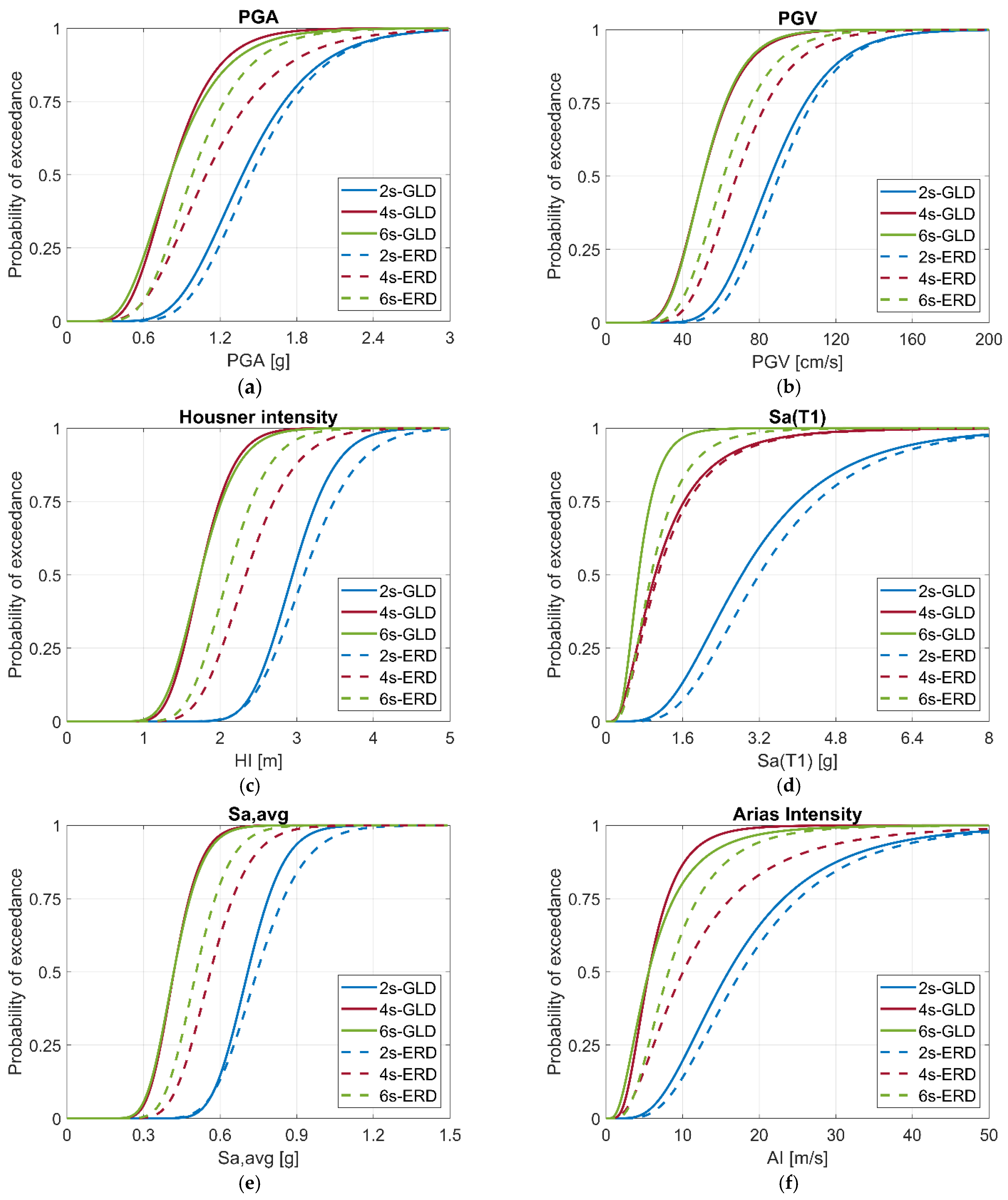
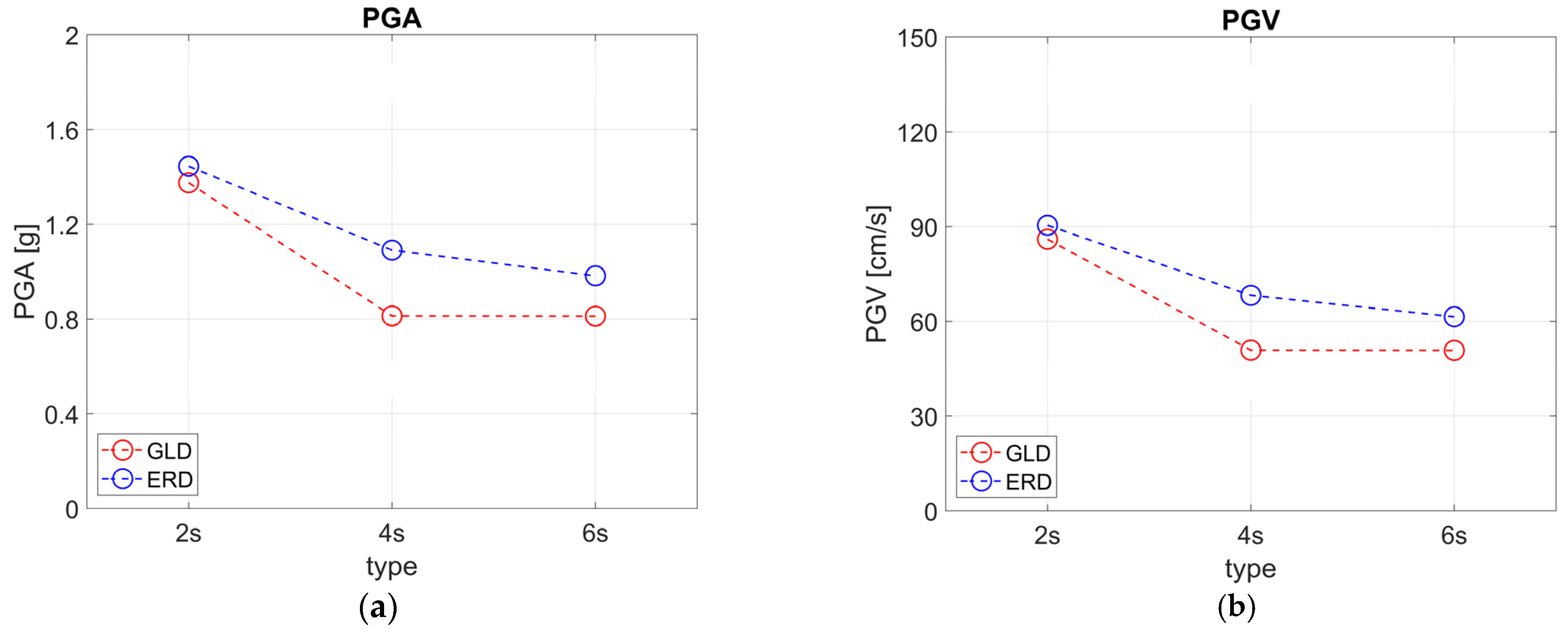
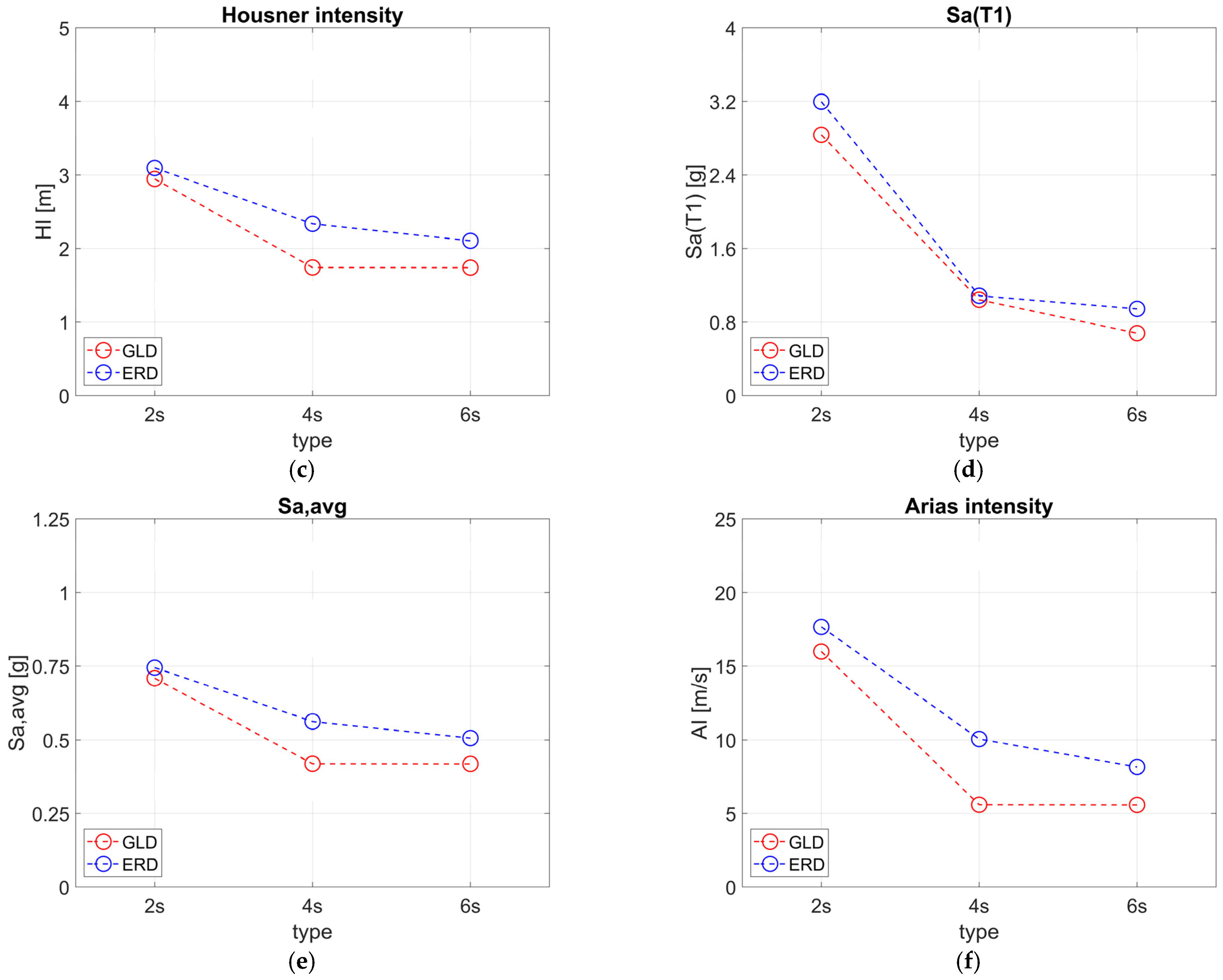
• As expected, for all IMs, ERD types exhibit higher median values compared to GLD ones, with more significant differences observed for 4s and 6s types (in the range of about 20–80%). Lower differences are found for 2s types (in the range of about 5–10%).
• The median values for 2s are higher than those for 4s and 6s, which have similar values. The differences between 2s and 4–6s types are about 40% for GLD and 25% for ERD for all IMs, except for Sa(T1) and AI, which exhibit greater differences (in the range of about 43–66%).
• For GLD types, the median values in the X direction are always higher than those in the Y direction across all the considered IMs, whereas ERD types exhibit the opposite trend.
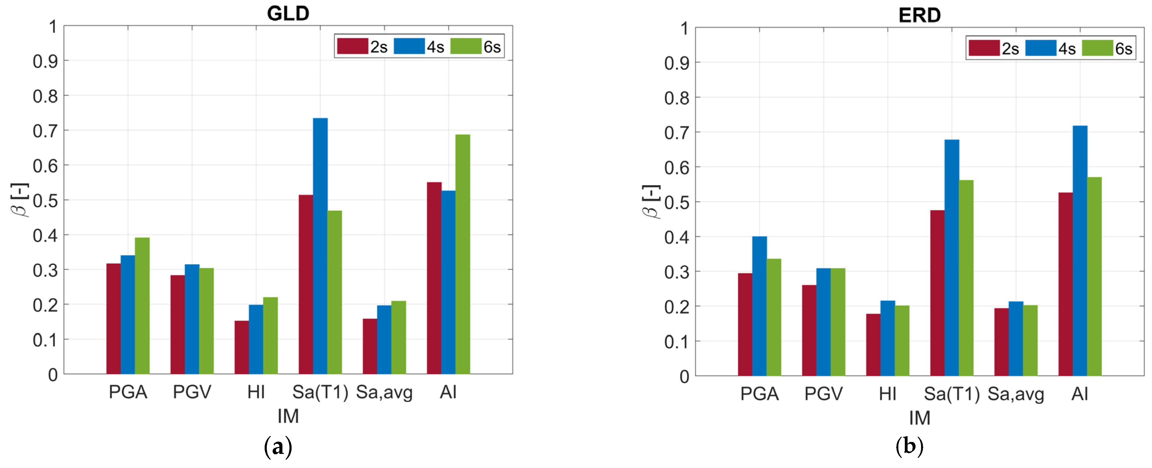
• The lowest dispersion values are found for HI (0.15–0.22) and Sa,avg (0.16–0.22), revealing greater efficiency compared to the other IMs such as Sa(T1) and AI, whose values are in the range 0.47–0.69 and 0.53–0.72, respectively.
• In general, the dispersion values slightly increase as the number of storeys increases without any significant differences between GLD and ERD types.

Further collapse analyses are currently being carried out involving other types such as retrofitted and modern anti-seismic RC buildings. The obtained results will allow for the vulnerability assessment of the most common building types to be used in seismic risk analyses.

References

1. Villaverde, R. Methods to assess the seismic collapse capacity of building structures: State of the art. J. Struct. Eng. 2007, 133, 57–66. [Google Scholar] [CrossRef]
2. Adam, C.; Ibarra, L.F. Seismic Collapse Assessment. In Encyclopedia of Earthquake Engineering; Beer, M., Kougioumtzoglou, I., Patelli, E., Au, I.K., Eds.; Springer: Berlin/Heidelberg, Germany, 2014. [Google Scholar] [CrossRef]
3. Lignos, D.; Krawinkler, H. Sidesway Collapse of Deteriorating Structural Systems Under Seismic Excitations; Report No. 177/2012; The John A. Blume Earthquake Engineering Center, Department of Civil and Environmental Engineering, Stanford University: Stanford, CA, USA, 2012. [Google Scholar]
4. Galanis, P.H.; Moehle, J.P. Development of collapse indicators for risk assessment of older-type reinforced concrete buildings. Earthq. Spectra 2015, 31, 1991–2006. [Google Scholar] [CrossRef]
5. Del Gaudio, C.; Ricci, P.; Verderame, G.M.; Manfredi, G. Urban-scale seismic fragility assessment of RC buildings subjected to L’Aquila earthquake. Soil. Dyn. Earthq. Eng. 2017, 96, 49–63. [Google Scholar] [CrossRef]
6. Gaetani d’Aragona, M.; Polese, M.; Prota, A. Seismic fragility curves for infilled RC building classes considering multiple sources of uncertainty. Eng. Struct. 2024, 321, 118888. [Google Scholar] [CrossRef]
7. Terrenzi, M.; Spacone, E.; Camata, G. Collapse limit state definition for seismic assessment of code-conforming RC buildings. Int. J. Adv. Struct. Eng. 2018, 10, 325–337. [Google Scholar] [CrossRef]
8. Federal Emergency Management Agency. Hazus Earthquake Model-Technical manual Hazus 6.1.; Department of Homeland Security, Federal Emergency Management Agency, Mitigation Division: Washington, DC, USA, 2024.
9. Celik, O.C.; Ellingwood, B.R. Seismic fragilities for non-ductile reinforced concrete frames—Role of aleatoric and epistemic uncertainties. Struct. Saf. 2010, 32, 1–12. [Google Scholar] [CrossRef]
10. Erberik, M.A. Fragility-based assessment of typical mid-rise and low-rise RC buildings in Turkey. Eng. Struct. 2008, 30, 1360–1374. [Google Scholar] [CrossRef]
11. Ghobarah, A. On drift limits associated with different damage levels. In Proceedings of the International Workshop on Performance-Based Seismic Design, Bled, Slovenia, 28 June–1 July 2004. [Google Scholar]
12. Rossetto, T.; Elnashai, A. Derivation of vulnerability functions for European-type RC structures based on observational data. Eng. Struct. 2003, 25, 1241–1263. [Google Scholar] [CrossRef]
13. Kappos, A.J.; Panagopoulos, G. Fragility curves for R/C buildings in Greece. Struct. Infrastruct. Eng. 2010, 6, 39–53. [Google Scholar] [CrossRef]
14. Ricci, P.; Manfredi, V.; Noto, F.; Terrenzi, M.; Petrone, C.; Celano, F.; De Risi, M.T.; Camata, G.; Franchin, P.; Magliulo, G.; et al. Modeling and seismic response analysis of Italian code-conforming reinforced concrete buildings. J. Earthq. Eng. 2018, 22 (Suppl. S2), 105–139. [Google Scholar] [CrossRef]
15. Vamvatsikos, D.; Cornell, C.A. Incremental dynamic analysis. Earthq. Eng. Struct. Dyn. 2002, 31, 491–514. [Google Scholar] [CrossRef]
16. Baker, J.W.; Cornell, C.A. Spectral shape, epsilon and record selection. Earthq. Eng. Struct. Dyn. 2006, 35, 1077–1095. [Google Scholar] [CrossRef]
17. Krawinkler, H.; Lignos, D.G. How to Predict the Probability of Collapse of Non-Ductile Building Structures. In Seismic Risk Assessment and Retrofitting. Geotechnical, Geological and Earthquake Engineering; Ilki, A., Karadogan, F., Pala, S., Yuksel, E., Eds.; Springer: Dordrecht, The Netherlands, 2009. [Google Scholar]
18. Haselton, C.B.; Deierlein, G.G. Assessing Seismic Collapse Safety of Modern Reinforced Concrete Moment Frame Buidings; Report n. 156 February 2007; The John A. Blume Earthquake Engineering Centre, Standford University: Stanford, CA, USA, 2007. [Google Scholar]
19. Liel, A.B.; Haselton, C.B.; Deierlein, G.G. Seismic Collapse Safety of Reinforced Concrete Buildings. II: Comparative Assessment of Nonductile and Ductile Moment Frames. J. Struct. Eng. 2011, 137, 492–502. [Google Scholar] [CrossRef]
20. Miano, A.; Jalayer, F.; Ebrahimian, H.; Prota, A. Cloud to IDA: Efficient fragility assessment with limited scaling. Earthq. Engng Struct. Dyn. 2018, 47, 1124–1147. [Google Scholar] [CrossRef]
21. Ibarra, L.F.; Medina, R.A.; Krawinkler, H. Hysteretic models that incorporate strength and stiffness deterioration. Earthq. Eng. Struct. Dyn. 2005, 34, 489–1511. [Google Scholar] [CrossRef]
22. Goulet, C.A.; Haselton, C.B.; Mitrani-Reiser, J.; Beck, J.L.; Deierlein, G.G.; Porter, K.A.; Stewart, J.P. Evaluation of the seismic performance of a code-conforming reinforced-concrete frame building—From seismic hazard to collapse safety and economic losses. Earthq. Engng Struct. Dyn. 2007, 36, 1973–1997. [Google Scholar] [CrossRef]
23. Haselton, C.B.; Baker, J.W. Ground Motion Intensity Measures for Collapse Capacity Prediction: Choice of Optimal Spectral Period and Effect of Spectral Shape. In Proceedings of the 8th National Conference on Earthquake Engineering, San Francisco, CA, USA, 18–22 April 2006. [Google Scholar]
24. Zhou, J.; Zhang, Z.; Williams, T.; Kunnath, S.K. Challenges in Evaluating Seismic Collapse Risk for RC Buildings. Int. J. Concr. Struct. Mater. 2021, 15, 27. [Google Scholar] [CrossRef]
25. Shome, N.; Cornell, C.A. Probabilistic Seismic Demand Analysis of Nonlinear Structures; Report No. RMS-35; RMS Program, Stanford University: Stanford, CA, USA, 1999. [Google Scholar]
26. Kiani, J.; Camp, C.; Pezeshk, S. On the number of required response history analyses. Bull. Earthq. Eng. 2018, 16, 5195–5226. [Google Scholar] [CrossRef]
27. Sattar, S.; Liel, A.B. Seismic Performance of Nonductile Reinforced Concrete Frames with Masonry Infill Walls—II: Collapse Assessment. Earthq. Spectra 2016, 32, 819–842. [Google Scholar] [CrossRef]
28. Iervolino, I.; Baraschino, R.; Spillatura, A. Evolution of seismic reliability of code-conforming Italian buildings. J. Earthq. Eng. 2023, 27, 1740–1768. [Google Scholar] [CrossRef]
29. Pavel, F. Collapse Assessment for Code-Conforming Reinforced Concrete Frame Structures in Romania. Front. Built Environ. 2018, 4, 50. [Google Scholar] [CrossRef]
30. Di Domenico, M.; De Risi, M.T.; Manfredi, V.; Terrenzi, M.; Camata, G.; Mollaioli, F.; Noto, F.; Ricci, P.; Franchin, P.; Masi, A.; et al. Modelling and seismic response analysis of Italian pre-code and low-code reinforced concrete buildings. Part II: Infilled Frames. J. Earthq. Eng. 2022, 27, 1534–1564. [Google Scholar] [CrossRef]
31. Shokrabadi, M.; Banazadeh, M.; Shokrabadi, M.; Mellati, A. Assessment of seismic risks in code conforming reinforced concrete Frames. Eng. Struct. 2015, 98, 14–28. [Google Scholar] [CrossRef]
32. Noh, N.M.; Tesfamariam, S. Seismic Collapse Risk Assessment of Code-Conforming RC Moment Resisting Frame Buildings Designed with 2014 Canadian Standard Association Standard A23.3. Front. Built Environ. 2018, 4, 53. [Google Scholar] [CrossRef]
33. De Risi, M.T.; Di Domenico, M.; Manfredi, V.; Terrenzi, M.; Camata, G.; Mollaioli, F.; Noto, F.; Ricci, P.; Franchin, P.; Masi, A.; et al. Modelling and seismic response analysis of Italian pre-code and low-code reinforced concrete buildings. Part I: Bare Frames. J. Earthq. Eng. 2022, 27, 1482–1513. [Google Scholar] [CrossRef]
34. Manfredi, V.; Masi, A.; Nicodemo, G.; Digrisolo, A. Seismic fragility curves for the Italian RC residential buildings based on non linear dynamic analyses. Bull. Earthq. Eng. 2023, 21, 2173–2214. [Google Scholar] [CrossRef]
35. Masi, A.; Lagomarsino, S.; Dolce, M.; Manfredi, V.; Ottonelli, D. Towards the updated Italian seismic risk assessment: Exposure and vulnerability modelling. Bull. Earthq. Eng. 2021, 19, 3253–3286. [Google Scholar] [CrossRef]
36. Italian National Institute of Statistics, ISTAT. Website and Data Warehouse 2011. Available online: https://www.istat.it/ (accessed on 11 March 2025). (In Italian)
37. Law n. 1086, 5 November 1971. Norme per la disciplina delle opere di conglomerato cementizio armato, normale e precompresso ed a struttura metallica. Official Journal n. 321, 21 December 1971. (In Italian)
38. Law n. 64, 2 February 1974. Provvedimenti per le costruzioni con particolari prescrizioni per le zone sismiche. Official Journal n. 76, 21 March 1974. (In Italian)
39. Royal Decree n. 2229, 16 November 1939. Norme per l’accettazione dei leganti idraulici. Official Journal n.92, 18 April 1940. (In Italian)
40. Law n. 1684 25 November 1962. Provvedimenti per l’edilizia, con particolari prescrizioni per le zone sismiche. Official Journal n. 326, 25 November 1962. (In Italian)
41. Royal Law Decree n. 640, 25 March 1935. Nuovo testo delle norme tecniche di edilizia con speciali prescrizioni per le localita colpite dai terremoti. Official Journal n. 120, 22 May 1935. (In Italian)
42. Ordinance of the President of the Council of Ministers (OPCM) 20 March 2003, n.3274, Official Journal n. 72, 8 May 2003. (In Italian)
43. Manfredi, V.; Masi, A. Seismic Strengthening and Energy Efficiency: Towards an Integrated Approach for the Rehabilitation of Existing RC Buildings. Buildings 2018, 8, 36. [Google Scholar] [CrossRef]
44. Masi, A. Seismic vulnerability assessment of gravity load designed R/C frames. Bull. Earthq. Eng. 2003, 1, 371–395. [Google Scholar] [CrossRef]
45. Ministerial Decree 30 May 1972. Norme tecniche alle quali devono uniformarsi le costruzioni in conglomerato cementizio, normale e precompresso ed a struttura metallica. Official Journal n. 190 22 July 1972. (In Italian)
46. McKenna, F. OpenSees: A framework for earthquake engineering simulation. Comput. Sci. Eng. 2011, 13, 58–66. [Google Scholar] [CrossRef]
47. Haselton, C.B.; Liel, A.B.; Lange, S.T.; Deierlein, G.G. Beam-Column Element Model Calibrated for Predicting Flexural Response Leading to Global Collapse of RC Frame Buildings; PEER Report No. 2007/03; University of California: Berkeley, CA, USA, 2008. [Google Scholar]
48. Sezen, H.; Moehle, J.P. Shear strength model for lightly reinforced concrete columns. J. Struct. Eng. 2004, 130, 1692–1703. [Google Scholar] [CrossRef]
49. Decanini, L.D.; Fantin, G.E. Modelos simplificados de la mampostería incluidas en porticos. Características de rigidez y resistencia lateral en estado límite. In Proceedings of the Actas de las VI Jornadas Argentinas de Ingenieria Estructural, Buenos Aires, Argentina, 1–3 October 1986; Volume 2, pp. 817–836. [Google Scholar]
50. Ricci, P.; Manfredi, V.; Noto, F.; Terrenzi, M.; De Risi, M.T.; Di Domenico, M.; Camata, G.; Franchin, P.; Masi, A.; Mollaioli, F.; et al. RINTC-e: Towards seismic risk assessment of existing residential reinforced concrete buildings in Italy, In Proceedings of the COMPDYN 2019-7th International Conference on Computational Methods in Structural Dynamics and Earthquake Engineering, Crete, Greece, 24–26 June 2019.
51. Masi, A.; Digrisolo, A.; Santarsiero, G. Analysis of a Large Database of Concrete Core Tests with Emphasis on Within-Structure Variability. Materials 2019, 12, 1985. [Google Scholar] [CrossRef] [PubMed]
52. Verderame, G.M.; Ricci, P.; Esposito, M.; Manfredi, G. STIL v1.0—Software per la caratterizzazione delle proprietà meccaniche degli acciai da c.a. tra il 1950 e il 2000. ReLUIS, Naples, Italy. Available online: http://www.reluis.it/ (accessed on 10 February 2025).
53. Calvi, G.M.; Bolognini, D. Seismic response of reinforced concrete frames infilled with weakly reinforced masonry panels. J. Earthq. Eng. 2001, 5, 153–185. [Google Scholar] [CrossRef]
54. Jalayer, F.; Cornell, C.A. Alternative non-linear demand estimation methods for probability-based seismic assessments. Earthq. Eng. Struct. Dyn. 2009, 38, 951–972. [Google Scholar] [CrossRef]
55. Cornell, C.A.; Jalayer, F.; Hamburger, R.O.; Foutch, D.A. Probabilistic basis for 2000 SAC Federal Emergency Management Agency steel moment frame guidelines. J. Struct. Eng. (ASCE) 2002, 128, 526–533. [Google Scholar] [CrossRef]
56. Zacharenaki, A.; Fragiadakis, M.; Assimaki, D.; Papadrakakis, M. Bias assessment in Incremental Dynamic Analysis due to record scaling. Soil. Dyn. Earthq. Eng. 2014, 67, 158–168. [Google Scholar] [CrossRef]
57. Vamvatsikos, D.; Cornell, C.A. Applied incremental dynamic analysis. Earthq. Spectra 2004, 20, 523–553. [Google Scholar] [CrossRef]
58. Smerzini, C.; Galasso, C.; Iervolino, I.; Paolucci, R. Ground motion record selection based on broadband spectral compatibility. Earthq. Spectra 2014, 30, 1427–1448. [Google Scholar] [CrossRef]
59. Manfredi, V.; Masi, A.; Özcebe, A.G.; Paolucci, R.; Smerzini, C. Selection and spectral matching of recorded ground motions for seismic fragility analyses. Bull. Earthq. Eng. 2022, 20, 4961–4987. [Google Scholar] [CrossRef]
60. Ministrial Decree 17 January 2018, NTC 2018. Aggiornamento delle “Norme Tecniche per le Costruzioni”. Official Journal n. 42, 20 February 2018. (In Italian)
61. Kazantzi, A.K.; Vamvatsikos, D. Intensity measure selection for vulnerability studies of building classes. Earthq. Eng. Struct. Dyn. 2015, 44, 2677–2694. [Google Scholar] [CrossRef]
62. Porter, K.; Kennedy, R.; Bachman, R. Creating Fragility Functions for Performance-Based Earthquake Engineering. Earthq. Spectra 2007, 23, 471–489. [Google Scholar] [CrossRef]
63. Baker, J.W. Efficient analytical fragility function fitting using dynamic structural analysis. Earthq. Spectra 2015, 31, 579–599. [Google Scholar] [CrossRef]
64. O’Reilly, G.J. Limitations of Sa(T1) as an intensity measure when assessing non-ductile infilled RC frame structures. Bull. Earthq. Eng. 2021, 19, 2389–2417. [Google Scholar] [CrossRef]
Figure 1. Flowchart of the study.
Buildings 15 01263 g001
Figure 2. Italian building stock: distribution in terms of number of storeys (a) and design levels (b). Adapted from [34].
Buildings 15 01263 g002
Figure 3. Three-dimensional view for 2- (a), 4- (b), 6-storey types (c) and in-plane layout considered for 2-storey (d) and for 4-6-storey types (e).
Buildings 15 01263 g003aBuildings 15 01263 g003b
Figure 4. M–θ relationships (in green) in the cases of flexural failure (a), shear failure (b) and intermediate (flexural/shear) failure (c), evaluated as a function of the shear capacity function (in red).
Buildings 15 01263 g004
Figure 5. Equivalent strut model (a) and in-plane response for the strut (b).
Buildings 15 01263 g005
Figure 6. Median IDA curves for 2s (a), 4s (b) and 6s (c) types.
Buildings 15 01263 g006
Figure 7. IDA curves (in black) for the X direction of the 4s-GLD type, along with the lognormal distribution function (in blue) fitted for the IDR values at collapse (black squares with a red marker edge).
Buildings 15 01263 g007
Figure 8. IDR profiles for 2s-, 4s-, and 6s-GLD types along the X (ac) and Y (df) directions.
Buildings 15 01263 g008aBuildings 15 01263 g008b
Figure 9. Fragility curve (red line) in terms of PGA derived from the cumulative fractions of collapse (black squares with a red marker edge), derived for the 4s-GLD type.
Buildings 15 01263 g009
Figure 10. Median values eµ for all the considered types in terms of PGA (a), PGV (b), HI (c), Sa(T1) (d), Sa,avg (e), and AI (f).
Buildings 15 01263 g010aBuildings 15 01263 g010b
Figure 11. Values of dispersion β for all the considered IMs, separately for GLD (a) and ERD (b) types.
Buildings 15 01263 g011