A Mindlin-Based Improved Newmark Method for the Seismic Stability of Anchored Slopes with Group Anchor Effects

Abstract

As the lifespan of many anchored slope reinforcements in China approaches its end, there is an increased need for secondary reinforcement. This study addresses the interaction between new and existing anchors, a critical but challenging aspect. The study introduces the Anchor Rod Modified Newmark Sliding Block Method (AMNB), which enhances the traditional Newmark Sliding Block Method (NSBM) by incorporating maximum anchor rod tension, dynamic tension changes, and group anchor effects. This improvement enhances the prediction of seismic displacement in slopes with multiple anchors. The AMNB method represents an innovation in slope stability analysis, as it is the first to integrate these dynamic and interactive factors into a unified framework. Validation through comparison with established seismic permanent displacement calculations and the analysis of three typical seismic motions show the AMNB’s effectiveness in capturing dynamic behaviors under seismic excitation. Additionally, numerical simulations using FLAC3D were conducted to validate the proposed method. The results indicate that considering group anchor effects and dynamic tension changes reduces the predicted seismic permanent displacement by up to 10% compared to traditional methods. The proposed AMNB method aligns more closely with the numerical simulation results. The findings indicate that group anchor effects negatively impact anchor forces, dynamic yield accelerations, and seismic displacements, leading to lower anchor tensions and dynamic yield accelerations. This, in turn, results in larger final slope permanent displacements under the same conditions.

1. Introduction

Since the 1950s, soil and rock anchoring technology has played a pivotal role in Chinese engineering, with applications spanning over tens of thousands of projects across the country [1]. However, as many of these anchored slopes near or exceed their intended service life, they encounter various challenges, including natural degradation, inadequate corrosion protection, and insufficient maintenance [2]. These issues are further compounded by changes in site conditions due to human activities, such as additional loading or excavations, which can exacerbate stability problems. The combined effects of aging infrastructure and changing site conditions often result in insufficient support force from anchor rods, potentially compromising slope stability.

When the safety of existing anchoring projects is compromised, effective reinforcement measures become imperative. According to the “Technical Code for Building Slope Engineering” [3], one of the most recognized methods for reinforcing slopes is the addition of new anchor rods to existing walls. However, this approach introduces new design challenges, particularly in high-density configurations where the reduced spacing between new and existing anchor rods may not comply with current standards. The interaction between new and existing anchors is a critical factor that significantly influences the overall system performance. Despite its acknowledged importance [4,5], there is a significant gap in the quantitative evaluation and integration of these interactions into design practices.

To address these challenges, it is crucial to continuously optimize slope stability analysis methods to adapt to the stability assessment of slopes after secondary reinforcement [1,6,7,8,9,10]. The dynamic response of slopes under strong seismic loading remains a key focus in geotechnical engineering. Seismic activity can cause significant damage to anchoring projects, leading to substantial losses in terms of safety and property. The seismic performance of geotechnical structures is typically evaluated from the perspectives of strength and deformation, with slope displacement being a critical aspect in assessing seismic stability [11,12].

Scholars have endeavored to establish seismic slope stability analysis methods from various perspectives, including the pseudo-static method, rigid block sliding method, model testing method, and other numerical simulation approaches. The pseudo-static method cannot account for the dynamic and cyclic nature of seismic loading, including temporal changes in ground motion during the seismic event. The physical model testing methods based on similarity theory allow for more realistic simulations of seismic effects on slopes [13]. Kuo-Lung Wang [6] adopted the shaking table model slope test for the study of slope failure initiation based on analyses of limit equilibrium, particle image velocimetry (PIV) analysis, and acceleration time history recorded within the model slope. Liping Wang [14] conducted dynamic centrifuge model tests to investigate the dynamic response of cohesive soil slopes with the use of stabilizing piles during an earthquake. The behavior of the pile reinforcement was analyzed based on the obtained deformation over the entire slope through image-based measurement, and the behavior of the slope was compared to that of an unreinforced slope. These methods effectively simulate and analyze the dynamic response of prototype slopes. However, they face challenges in selecting model materials that meet all scaling laws and similarity criteria. Environmental factors and boundary conditions also significantly influence test results, and the method often requires substantial financial investment in specialized equipment.

Various scholars have employed numerical simulation approaches to analyze the seismic response process of slopes. For instance, Markus Goldgruber compared the qualitative possible and critical displacements of the Newmark’s sliding block analysis and a Fluid–Foundation–Structure Interaction simulation with the finite elements method. The conclusion is that Newmark Sliding Block Method (NSBM) [15] analysis and the finite elements simulation are only comparable for high friction angles [16]. Linlu Zhou employed Fast Lagrangian Analysis of Continua in Two Dimensions (FLAC2D) in the numerical simulation to explore the stability of the slope before and after treatment under earthquake action. The computed results show that the stability of the slope is greatly influenced by earthquakes, and the slope displacement under seismic conditions is far larger than that under natural conditions. Three treatment measures, including excavation, anti-slide piles, and anchor cables, can significantly reduce slope displacement and the internal force on anti-slide piles, and can improve the stability of a slope during an earthquake [17]. These methods effectively replicate actual deformations and consider factors like material non-linearity, discontinuities, and dynamic loading conditions. However, they are complex and sensitive to grid partitioning and parameter settings, requiring high proficiency from analysts. Their use is often limited to research professionals and less prevalent in practical engineering applications.

NSBM provides a more efficient approach for these limitations. This method simplifies the analysis by using rigid body motion equations for potential sliding masses, incorporating time-varying ground motions, and determining the cumulative permanent displacement of the slope during an earthquake. The method initially gained widespread application in the analysis of regional seismic slope stability, and it was rapidly extended to various types of slopes, including natural hillsides, engineered embankments, and earth dams; its applicability stems from its relatively simple yet effective formulation, clear physical interpretation, and the accessibility of the required input parameters [18,19]. Despite its widespread use, the traditional NSBM has limitations when applied to anchored slopes, particularly in its treatment of anchor forces during seismic events. The conventional approach makes key simplifications: the initial pre-stress is assumed to be constant and equal to the axial force in the anchor cables, and both the axial force in the anchors and the yield acceleration of the slope are considered invariant throughout the seismic event. Therefore, the yield acceleration is commonly regarded as a constant parameter in the conventional method to determine the seismic displacement of the slope [20,21]. However, research by Gordan et al. [22] has shown that structural discontinuities in rock masses significantly reduce their integrity, making them more susceptible to deformation and failure under seismic loading. As a result, support anchors (cables) often experience complex and varying tensile-shear forces during seismic events, leading to substantial fluctuations in their axial forces [10]. To more accurately reflect the true seismic displacement behavior, they established a dynamic mechanics failure mechanism and instantaneous displacement model for pre-stressed anchor-reinforced slopes over infinitesimal time intervals. Based on the upper bound theorem, a time-dependent formula for dynamic yield acceleration was derived and a modified method for determining the seismic permanent displacement was proposed. However, the influence of the maximum axial force of the anchor is neglected. In extreme cases, these force variations may exceed the ultimate anchoring capacity, potentially leading to anchor failure or the significant loss of stabilizing forces. On the other hand, as mentioned earlier, the effect of group anchor interaction in secondarily reinforced slopes cannot be ignored. Therefore, considering the dynamic changes in the axial forces of pre-stressed anchor bolts, the impact of the maximum axial force and group anchor effects is crucial for the accurate seismic design and risk assessment of anchored slopes.

Despite the widespread use of anchoring technology in slope stabilization, there remains a significant gap in the quantitative evaluation of the interaction between new and existing anchors, particularly in high-density configurations. Traditional methods, such as the conventional NSBM and the pseudo-static approach [23], often assume constant anchor forces and neglect the dynamic changes in tension during seismic events. Furthermore, the effects of group anchor interactions, which can significantly influence the overall stability of the slope, are rarely considered in design practices. These simplifications can lead to non-conservative stability assessments, potentially compromising the safety of engineering projects. To address these limitations, an AMNB method was developed to account for the maximum anchor rod tension and group anchor effects in slope stability analysis. The AMNB method provides a more accurate and practical tool for evaluating the seismic performance of anchored slopes, particularly in scenarios involving secondary reinforcement or limited anchor spacing. First, based on Mindlin’s solution in elastic mechanics, the method to calculate the maximum anchor rod tension and the group anchor effect coefficient was formulated. Then, building upon the traditional Newmark method and the proposed calculation method, the AMNB was established for slopes reinforced with multiple anchors, considering the constraints on the slope maximum anchor rod tension and the influence of group anchor effects. To validate the proposed AMNB method, numerical simulations were conducted using FLAC3D 6.0, a widely used software in geotechnical engineering for modeling the dynamic response of slopes under seismic loading. FLAC3D was chosen for its ability to accurately simulate complex geotechnical problems, including the interaction between anchor rods and the surrounding soil or rock mass, as well as for its robust handling of dynamic loading conditions. The use of FLAC3D provides a reliable benchmark for comparing the results of the AMNB method, ensuring the accuracy and robustness of the proposed approach. Finaly, a case study of a typical reinforced slope was conducted to validate the AMNB, comparing results with existing work. The results of this study demonstrate the effectiveness of the proposed AMNB method in improving the accuracy of seismic displacement predictions for anchored slopes. The study shows that anchor spacing of less than 3 m significantly reduces the forces on individual anchors due to group effects. Additionally, group anchor effects can reduce the maximum anchor rod force by up to 5.1%, and the presence of vertical seismic acceleration can increase the permanent displacement by up to 10%. These quantitative results highlight the importance of considering dynamic tension changes and group anchor effects in the design and analysis of anchored slopes under seismic conditions.

2. Theoretical Analysis Model

2.1. Analysis of Maximum Axial Force in Anchor Cables

The Mindlin displacement solution [24] is a fundamental theoretical framework for understanding stress and displacement distributions in elastic media. The Mindlin solution has significant advantages in solving the deformation and stress distribution problems caused by concentrated forces in elastic media, especially when considering the interaction between anchors and surrounding soil or rock. Compared with other solutions, the Mindlin solution can more accurately describe the stress and displacement distributions at greater depths and has more advantages in deformation analysis under the action of multiple forces. This is very important for the multi-anchor effect and dynamic response considered in our research [25]. Therefore, the Mindlin solution is used to further construct the effect of group anchorage effect on the axial force of bolts. Mindlin developed this solution to address the problem of deformations and stresses induced within a semi-infinite elastic medium subjected to a concentrated force. The solution is based on the following key assumptions:

(a)

The medium is homogeneous and isotropic.

(b)

The material behavior is linearly elastic.

(c)

The medium is semi-infinite in extent.

(d)

Gravitational effects are neglected.

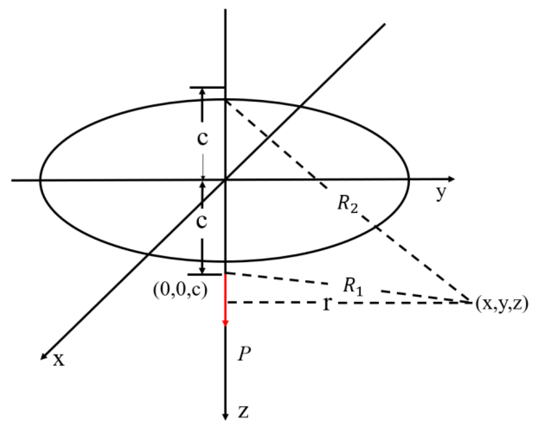
As shown in Figure 1, the solution considers a vertically concentrated force P applied at a point within the medium, at a depth c below the free surface. The solution provides the vertical displacement and vertical stress ${\tau }_{\mathrm{rz}}$ induced at various points in three-dimensional space due to the concentrated load.

$$w={\displaystyle \frac{P(1+\nu )}{8\pi E(1-\nu )}}{\displaystyle \frac{3-4\nu }{R_1}}+{\displaystyle \frac{8{(1-\nu )}^2-(3-4\nu )}{R_2}}+{\displaystyle \frac{{(z-c)}^2}{R_1^3}}+{\displaystyle \frac{(z-4\nu ){(z+c)}^2-2cz}{R_2^3}}+{\displaystyle \frac{6cz{(z+c)}^2}{R_2^3}}$$

(1)

$${\tau }_{rz}={\displaystyle \frac{Pr}{8\pi (1-\nu )}}[-{\displaystyle \frac{1-2\nu }{R_1^3}}+{\displaystyle \frac{1-2\nu }{R_2^3}}-{\displaystyle \frac{3{(z-c)}^2}{R_1^5}}-{\displaystyle \frac{3(3-4\nu )z(z+c)-3c(3z+c)}{R_2^5}}-{\displaystyle \frac{30cz{(z+c)}^2}{R_2^5}}]$$

(2)

In the above equations, the following applies:

$$R_1=\sqrt{x^2+y^2+{(z-c)}^2}$$

(3)

$$R_2=\sqrt{x^2+y^2+{(z+c)}^2}$$

(4)

E represents the elastic modulus of the rock and soil, and ν denotes the Poisson’s ratio of the surrounding rock and soil in the anchored segment.

Assume that the rock and soil within the range of anchor cable action are linearly elastic, uniformly isotropic, and semi-infinite, and the anchor body is a linearly elastic body. The plane z = 0 is taken as the plane passing through the near end of the anchor body and perpendicular to the anchor rod. The anchor cable is assumed to deform compatibly with the surrounding rock and soil mass under applied stresses, and the grouting body of the anchored segment is assumed to maintain constant material properties throughout the loading process. Under the action of pre-stress loads in the semi-infinite rock mass, lateral frictional resistance ${\tau }_Z$ is generated along the interface between the anchored segment and the surrounding medium. The following is given according to Equation (1), when x = y = z = 0:

$$W={\displaystyle \frac{2\pi a{\tau }_z(1+\nu )(3-2\nu )}{2Ec}}$$

(5)

In the linear elastic stage, the deformation occurring within the anchorage section itself is as follows:

$$W_a={\displaystyle {\int }_0^{L_m}}{\displaystyle \frac{1}{E_{a}A}}(P-2\pi a{\displaystyle {\int }_0^{L_m}}{\tau }_{z}dz)dz$$

(6)

Here, G, ν represent the shear modulus and Poisson’s ratio of the rock and soil mass, respectively. $E_a, A$, a are the elastic modulus, cross-sectional area, and radius of the anchor rod, respectively. P denotes the applied pre-stress load. The point z = 0 is the starting point of the shear stress distribution and the near end of the anchored segment, and $L_m$ is the length of the anchored segment at the far end.

Expressing Equation (6), and then taking the third derivative with respect to L for both sides, can simplify the resulting equation into a second-order, variable-coefficient homogeneous ordinary differential equation:

$${\tau }_z^{\prime \prime }+kz{\tau }_z^{\prime }+2k{\tau }_z=0$$

(7)

In the equation, the following applies:

$$k={\displaystyle \frac{4\pi G}{(3-2\nu )E_{a}A}}$$

(8)

The above equation is transformed as follows:

$${\tau }_z=\eta (\xi )exp\left({\displaystyle \frac{1}{4}}{\xi }^2\right)$$

(9)

$$z=-i{\displaystyle \frac{1}{\sqrt{k}}}\xi$$

(10)

Substituting them into Equation (8), the standard form of the Weber equation can be obtained [26]:

$$4{\eta }^{\prime }-({\xi }^2+3)\eta =0$$

(11)

The general solution to this equation is found to be as follows:

$$\eta =\xi e^{-{\displaystyle \frac{1}{2}}{\xi }^2}\left(c_1+c_2{\displaystyle \int \frac{1}{{\xi }^2}}\cdot e^{-{\xi }^2}d\xi \right)$$

(12)

Performing the inverse transformation on the above equation and incorporating the boundary conditions $\tau =$0 when L = 0 and $\tau =$0 as $L_m\to \infty$, the distribution function of the shear stress on the surface of the anchored segment can be obtained:

$${\tau }_z={\displaystyle \frac{Pt}{2\pi a}}\cdot z\cdot exp\left(-{\displaystyle \frac{1}{2}}t{z}^2\right)$$

(13)

In the equation, the following applies:

$$t={\displaystyle \frac{1}{(1+\nu )(3-2\nu )a^2}}\left({\displaystyle \frac{E}{E_a}}\right)$$

(14)

Taking the partial derivative of the shear stress with respect to z in Equation (14), the following is obtained:

$${\displaystyle \frac{\partial \tau }{\partial z}}={\displaystyle \frac{Pt}{\pi a}}[1-t{z}^2\cdot exp\left(-{\displaystyle \frac{1}{2}}t{z}^2\right)]$$

(15)

Setting ${\displaystyle \frac{\partial \tau }{\partial z}}=0$, have $z_0={\displaystyle \frac{1}{\sqrt{t}}}$. Therefore, when $z=z_0$, the maximum shear stress on the surface of the anchored segment can be obtained. Substituting $z_0$ into Equation (13), the following equation is obtained:

$${\tau }_{max}=exp\left(-{\displaystyle \frac{1}{2}}\right){\displaystyle \frac{p\sqrt{t}}{2\pi a}}$$

(16)

According to engineering practice, two primary force components act at the interface between the anchored segment and the surrounding rock and soil mass: (1) the normal force perpendicular to the surface of the anchored segment, and (2) the adhesive force on the surface of the anchored segment at the rock–soil interface. Therefore, Coulomb’s law can also be used to calculate the shear resistance between the anchored segment and the rock–soil interface:

$${\tau }_{max}=exp\left(-{\displaystyle \frac{1}{2}}\right)\cdot {\displaystyle \frac{P\sqrt{t}}{2\pi a}}\le \tau =c+\sigma tan\phi$$

(17)

$$P\le exp\left({\displaystyle \frac{1}{2}}\right){\displaystyle \frac{2\pi a}{\sqrt{t}}}\left(c+\sigma \tan \phi \right)$$

(18)

In the equation, c, $\phi$ represent the effective cohesive strength and internal friction angle of the rock and soil, respectively. $\sigma$ is the normal stress on the borehole wall.

Therefore, the maximum pull-out force of the anchor rod is given by the following:

$$P_{max}=exp\left({\displaystyle \frac{1}{2}}\right){\displaystyle \frac{2\pi a}{\sqrt{t}}}\left(c+\sigma \tan \phi \right)$$

(19)

2.2. Analysis of Group Anchor Effect on Anchor Cables

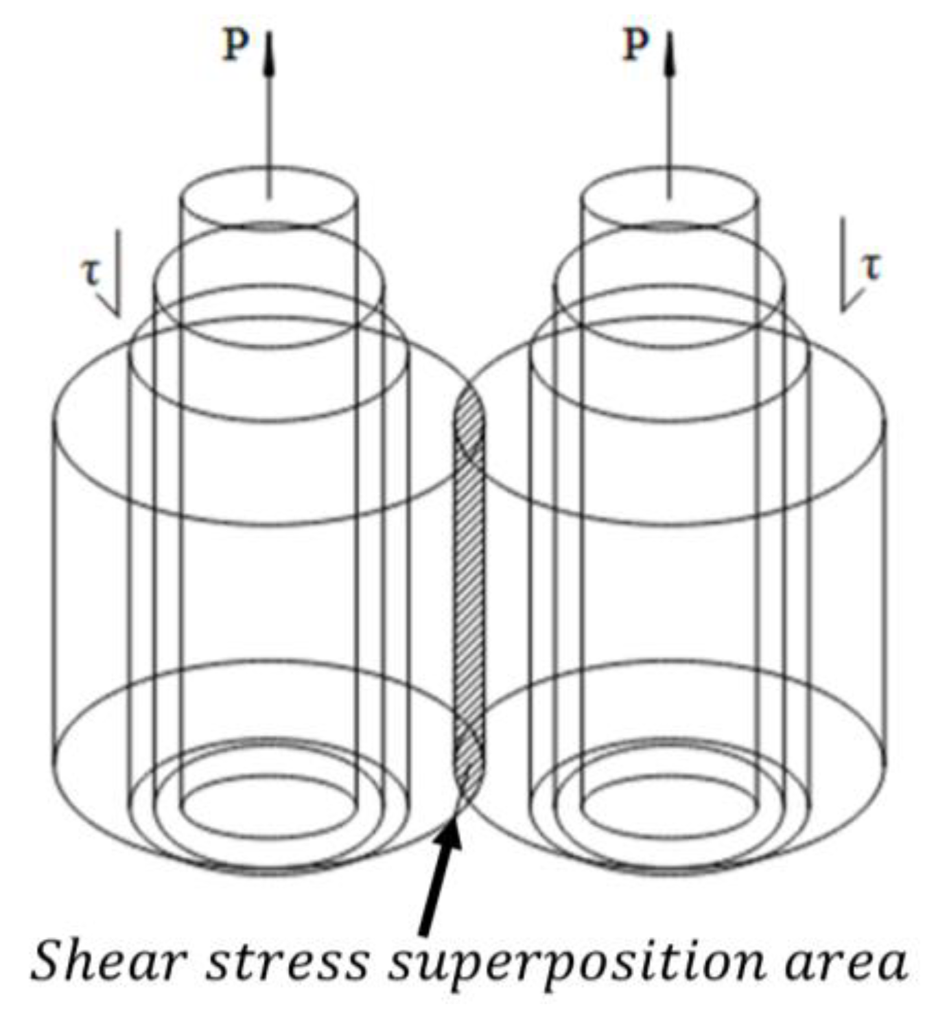
When anchor cables are subjected to pre-stress loads in semi-infinite rock and soil media, they primarily transfer these loads to the surrounding medium through shear forces generated along the surface of the anchoring sections. In situations where multiple anchor cables operate simultaneously, a complex three-dimensional shear stress field is formed within the surrounding rock and soil mass. If the spacing between anchor cables is insufficient, the individual shear stress fields may overlap and interact. 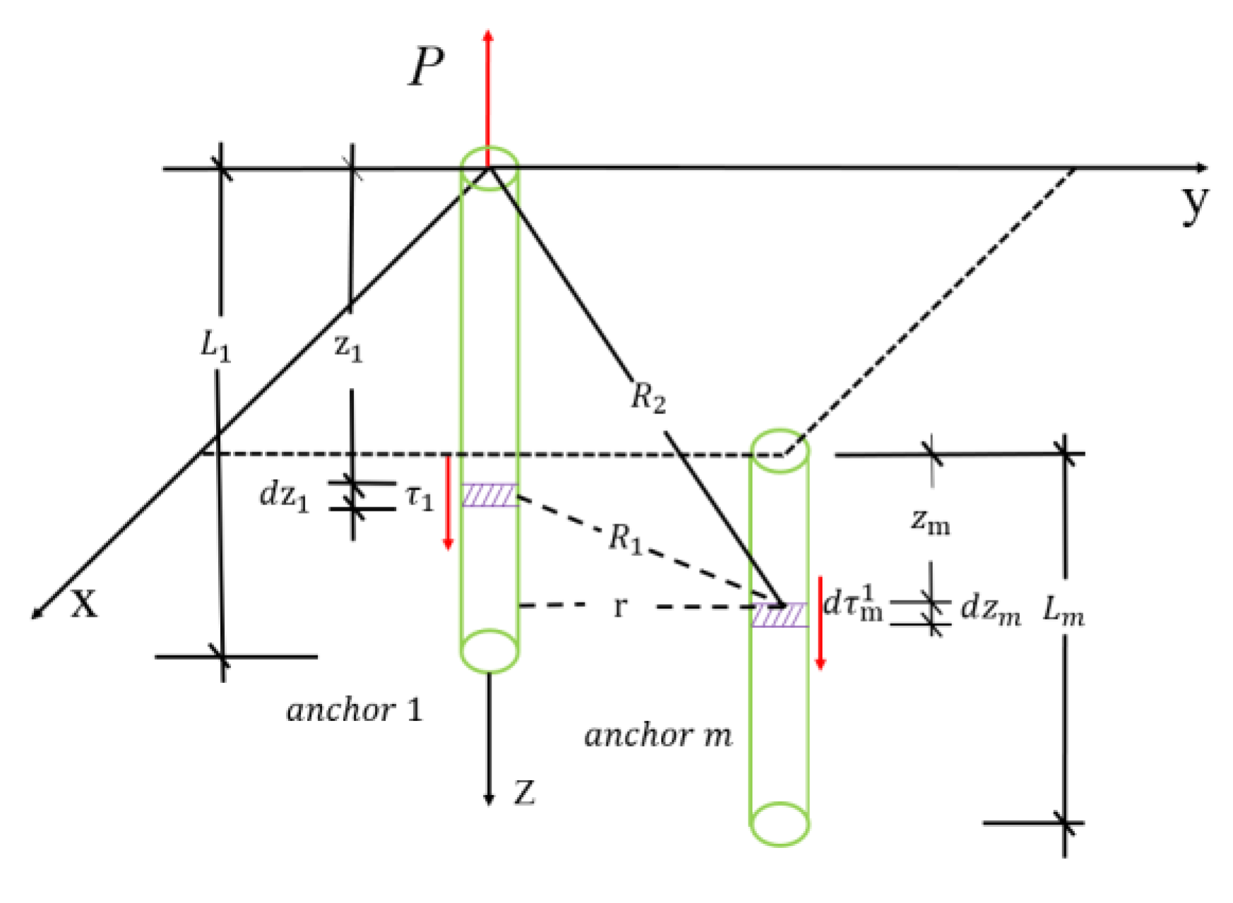This interaction can lead to stress concentrations and potentially cause shear failure in the anchored rock and soil mass, as illustrated in Figure 2. The superimposition of shear stresses between anchoring sections directly influences the load-carrying capacity of anchor groups. This interaction often results in a group efficiency factor, where the capacity of the group may be less than the sum of the individual anchor capacities. To accurately assess the group anchor effect, it is necessary to analyze the additional shear stresses that arise from the interaction between neighboring anchoring sections. These interaction stresses are distinct from the primary shear stresses developed around individual anchors. A differential element approach is used to study the distribution of shear stresses at any point within the rock and soil mass when loads act on arbitrary sections of the anchoring segments during the elastic phase. A micro-element of the anchoring section is isolated and a detailed mechanical analysis is conducted, as illustrated in Figure 3.

According to the aforementioned Formula (2), as shown in Figure 3, the differential shear stress $d{\tau }_m^1$ generated at any point in space by the micro-element anchoring section can be expressed as follows:

$$\begin{array}{l}d{\tau }_m^1={\displaystyle \frac{{\tau }_{1}2\pi ad{z}_{1}r}{8\pi (1-\nu )}}[-{\displaystyle \frac{1-2\nu }{R_1^3}}+{\displaystyle \frac{1-2\nu }{R_2^3}}-{\displaystyle \frac{3{(z_m-z_1)}^2}{R_1^5}}\\ -{\displaystyle \frac{3z_m(3-4\nu )(z_m+z_1)-3\mathrm{c}(3z_m+z_1)}{R_2^5}}+{\displaystyle \frac{30c{z}_m{(z_m+z_1)}^2}{R_1^5}}]\end{array}$$

(20)

This allows us to determine the additional shear stress ${\tau }_{\mathrm{m}}^1$ exerted by anchor rod 1 on another anchor rod m, where${\tau }_1$ can be obtained using Formula (7):

$$\begin{array}{l}{\tau }_m^1={\displaystyle {\int }_0^{L_m}{\displaystyle {\int }_0^{L_1}}}d{\tau }_m^1\cdot d{z}_m={\displaystyle {\int }_0^{L_m}{\displaystyle {\int }_0^{L_1}}}{\displaystyle \frac{ptar{z}_1\exp (-\frac{1}{2}t{z}_1^2)}{4\pi (1-\nu )d}}[-{\displaystyle \frac{1-2\nu }{R_1^3}}+{\displaystyle \frac{1-2\nu }{R_2^3}}\\ -{\displaystyle \frac{3{(z_m-z_1)}^2}{R_1^5}}-{\displaystyle \frac{3z_m(3-4\nu )(z_m+z_1)-3\mathrm{c}(3z_m+z_1)}{R_2^5}}+{\displaystyle \frac{30c{z}_m{(z_m+z_1)}^2}{R_1^5}}]\end{array}$$

(21)

In the bonded interface between the anchoring section and the surrounding rock and soil, two distinct components of shear stress emerge: the shear stress ${\tau }_{\mathrm{m}}$ generated by the anchor’s self-load and the additional shear stress ${\tau }_{\mathrm{m}}^1$ transmitted from the neighboring anchoring section’s shear stress field. The total shear stress acting on the anchoring section can be mathematically expressed as follows:

$$\tau ={\tau }_{\mathrm{m}}+{\tau }_{\mathrm{m}}^1$$

(22)

The anchoring force primarily results from the interaction forces, namely, the bonded surface shear stress, transmitted through the anchoring section by the pre-stressed loads of the anchor cables in the rock and soil. To facilitate the calculation of the anchoring section load capacity and to better characterize the situation of group anchor effects, the group anchor effect coefficient (denoted as φ) is introduced. This coefficient accounts for the interaction between multiple anchor rods in close proximity to one another. When anchors are placed too closely together, the shear stress fields generated around each anchor can overlap, leading to a reduction in their individual load-carrying capacities due to mutual interference. The group anchor effect coefficient quantifies this phenomenon by adjusting the predicted load capacity of the anchor cables, thus providing a more accurate representation of the actual forces acting on each anchor in a multi-anchor configuration. Let P represent the design load capacity of an anchor cable, assuming no group anchor effects. The actual load capacity of the anchor cable considering group anchor effects is denoted P′. The relationship between the design load capacity and the actual load capacity, incorporating the group anchor effect, can be expressed as follows:

$$\phi ={\displaystyle \frac{P^{\prime }}{P}}=1-{\displaystyle \frac{{\tau }_m^1}{{\tau }_m}}$$

(23)

The derivation process presented above is based on a model incorporating two anchor rods, which serves as a fundamental reference for analyzing anchoring systems. According to the principle of force superposition, it is evident that as the number of anchor rods increases beyond two, the group anchor effect coefficient can be generalized as follows:

$$\phi ={\displaystyle \frac{P^{\prime }}{P}}=1-{\displaystyle \frac{{\displaystyle \sum {\tau }_m^i}}{{\tau }_m}}i=1,2\dots \dots n$$

(24)

2.3. Physical Model

The stability of rocky slopes is governed by numerous factors, but in most cases, the primary factors affecting their stability, such as rock mass structural properties, groundwater, and topography, remain stable. However, when external forces, such as seismic actions, are applied, they can increase the downhill forces acting on the slope, thereby reducing its resistance to sliding. In these scenarios, the previously balanced stress relationships may be disrupted, leading to slope instability.

According to the NSBM theory, when seismic acceleration exceeds the yield acceleration, rigid soil begins to slide along the potential sliding surface. To determine the seismic permanent displacement of a pre-stressed anchored slope, an instantaneous displacement model was established within an infinitesimally small interval dt, as illustrated in the typical anchored rocky slope model in Figure 4. Reasonable assumptions were made for the model, assuming that tension cracks are located at the top of the slope and are upright. Given that rocky slopes often fail along joint surfaces, the sliding or failure surface is assumed to be a plane inclined at an angle θ that is less than the slope angle β. The potential sliding mass is considered completely rigid during the sliding process and is supported by multiple anchor rods. Using the pseudo-static method, seismic loads are simplified into horizontal and vertical inertial forces, with horizontal and vertical seismic acceleration coefficients denoted as $k_h$ and $k_v$, respectively. The vertical seismic component is assumed to be proportional to the horizontal seismic component, with their ratio represented by λ expressed mathematically as $K_v=\lambda \cdot K_h$. Parameters such as soil cohesion c, internal friction angle φ, and soil unit weight γ are assumed not to be affected by seismic loads.

2.4. Force Analysis

Considering seismic loads, slope top overload, and anchor tension, the force state at a given time during the seismic time history is illustrated in Figure 5. Due to the small displacement relative to the length of the sliding surface, the reduction in the length of the sliding surface is not considered. Based on geometric relationships, the lengths of the sliding surface $L_{OC}$, the weight of the sliding block W, the length of the slope top load $L_{AB}$, and the slope top load Q are given by the following:

$$L_{OC}={\displaystyle \frac{H-h}{sin\theta }}$$

(25)

$$W=0.5\gamma [(H^2-h^2)cot\theta -H^{2}cot\beta ]$$

(26)

$$Q=q{L}_{AB}=q\left[{\displaystyle \frac{0.5{\gamma }_w(H-h)}{tan\theta }}-{\displaystyle \frac{H}{tan\beta }}\right]$$

(27)

In the equation, H represents the slope height, h is the depth of the tension cracks, W denotes the weight of the sliding block, and q stands for the top overload.

The horizontal and vertical seismic forces are represented by $Q_h^{\mathrm{t}}$ and $Q_v^t$, respectively. Additionally, $K_h^t$ denotes the horizontal acceleration component coefficient of the seismic wave at time t, $K_v^t$ represents the vertical acceleration component coefficient at the same time, and $\xi$ is the ratio of the vertical to horizontal seismic acceleration coefficients. The equation can be expressed as follows:

$$Q_h^t=K_h^{t}W$$

(28)

$$Q_v^t=K_v^{t}W$$

(29)

$$K_v^t=\xi K_h^t$$

(30)

2.5. Dynamical Analysis of Anchor Cable

The initial pre-stress of the anchor cable is denoted as the initial pre-stress P, accounting for the group anchor effect. Given the small displacement of the slope relative to the length of the anchor rod during the seismic process, the inclination angle change of the anchor rod is ignored. It can be approximately assumed that the instantaneous sliding displacement increments $x_t$ within the time interval dt at time t is equal to the elongation of the anchor cable. Therefore, the axial force $P^t$ of the anchor cable at time t can be calculated by the following formula:

$$P^{\mathrm{t}}=\phi (P+\Delta P^{\mathrm{t}})$$

(31)

$$\Delta P^t={\displaystyle \frac{K_L{x}_t}{cos{\alpha }_i}}$$

(32)

The stiffness coefficient $K_L$ of the anchor rod, as specified in the Chinese standard “Technical Code for Building Slope Engineering” Article 8.2.6, for tension-type anchor rods, can be calculated using the following formula:

$$K_L={\displaystyle \frac{E_f{A}_f}{L_f}}$$

(33)

Here, $L_f$, $A_f$, and $E_f$ represent the free segment length, cross-sectional area of the free segment material, and the elastic modulus of the free segment material, respectively. Additionally, during the seismic process, the axial force in the anchor rod is constrained by the maximum anchoring force. Therefore, it can be expressed from Equation (18):

$$P^t\le exp\left({\displaystyle \frac{1}{2}}\right){\displaystyle \frac{2\pi a}{\sqrt{t}}}\left(c+\sigma \tan \phi \right)$$

(34)

2.6. Dynamic Safety Factor and Dynamic Yield Acceleration of the Slope

Considering the dynamic variation in the anchor rod tension, the instantaneous anti-sliding force $F_r^t$ of the slope block at time t within dt can be expressed as follows:

$$F_r^t=C_f{L}_{oc}+\left[\left(W+Q_v^t+Q\right)cos\theta +Q_h^{t}sin\theta -{\displaystyle \sum P_i^t}sin(\alpha +\theta )\right]tan{\phi }_f$$

(35)

In this equation, $C_f$ and ${\phi }_f$ represent the effective cohesive force and effective internal friction angle of the sliding surface, respectively. Similarly, the downslope force $F_i^t$ of the slope block is given by the following:

$$F_i^t=(W+Q_v^t+Q)sin\theta +Q_h^{t}cos\theta -{\displaystyle \sum P_i^t}cos(\alpha +\theta )$$

(36)

The dynamic safety factor $F_s^t$ of the slope during the seismic process can be defined as follows:

$$F_s^t={\displaystyle \frac{F_r^t}{F_i^t}}$$

(37)

When the dynamic safety factor is 1, the value of the seismic acceleration coefficient $k_h^t$ at that moment is the real-time yield acceleration coefficient of the slope, denoted as $k_y^t$.

2.7. Dynamical Permanent Displacement

This paper utilizes the NSBM proposed by Newmark to calculate the post-earthquake displacement of the slope. By cumulatively summing the seismic displacements at each time interval during seismic excitation, the seismic permanent displacement is expressed as follows. The rocky slope is considered a continuous, uniformly isotropic rigid body, and the reverse yield acceleration coefficient is assumed to be infinite. Therefore, when the input seismic wave acceleration coefficient $k_h^t$ is less than the slope’s yield acceleration $k_y^t$, the permanent displacement of the slope is zero. However, when the input seismic wave acceleration coefficient $k_h^t$ exceeds the slope’s yield acceleration $k_y^t$, acceleration along the sliding surface $x_t^{‘‘}$ is generated and can be calculated using the following formula:

$$x_t^{\prime \prime }={\displaystyle \frac{\left(k_h^t-k_y^t\right)gcos(\phi -\theta )}{cos\phi }}$$

(38)

According to the formula, integrating the acceleration twice yields the post-earthquake displacement x along the sliding surface, where n is the total number of instances when the input seismic wave acceleration coefficient $k_h^t$ exceeds the slope’s yield acceleration $k_y^t$.

$$x_{\mathrm{t}}={\displaystyle \sum _{t=0}^{n}d}{x}^i={\displaystyle \sum _{t=0}^n{\displaystyle {\int }_0^{dt}{\displaystyle {\int }_0^{dt}{x}_t^{\prime \prime }}}}dtdt$$

(39)

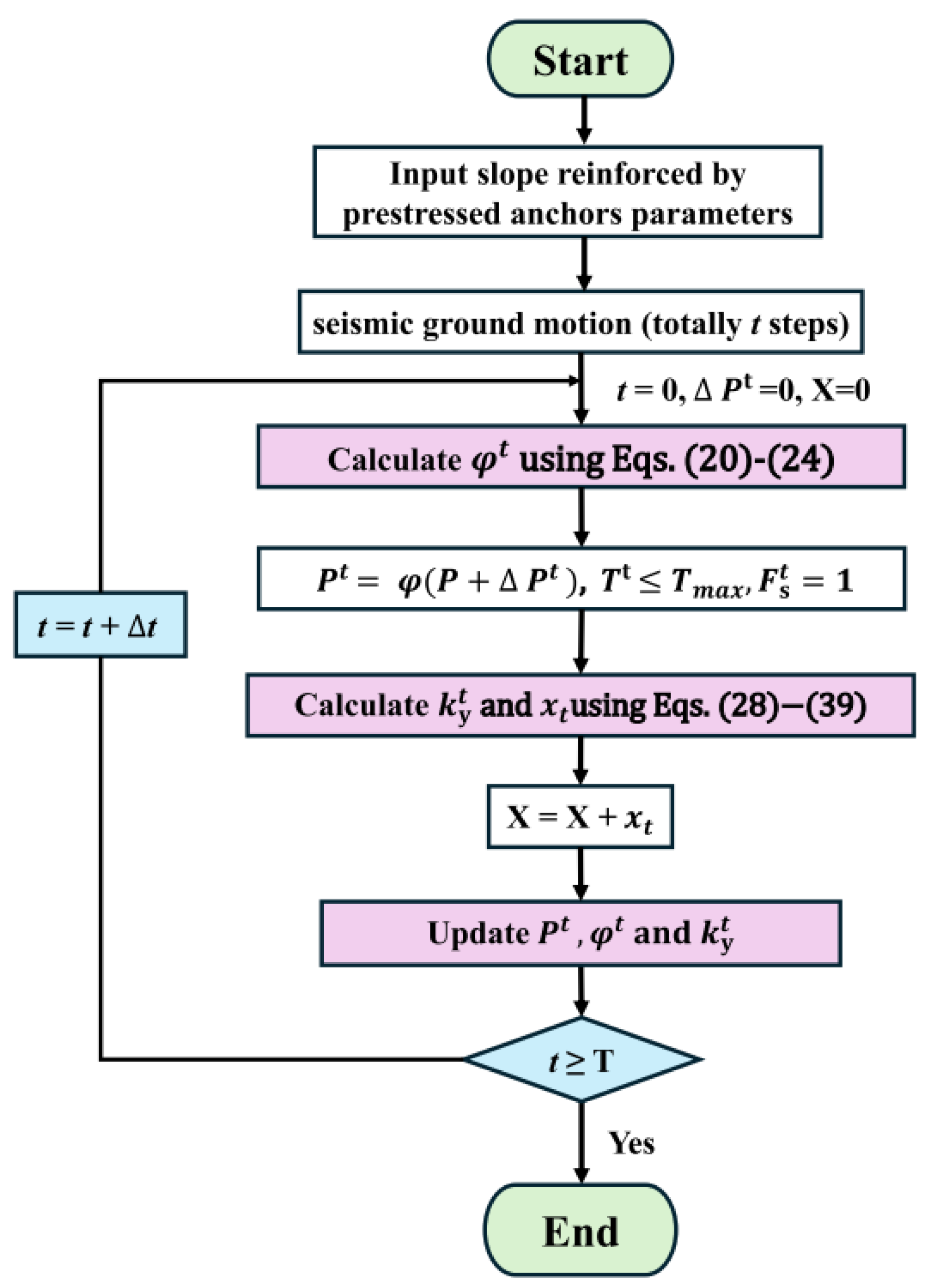
To provide a clearer presentation of the entire calculation process of the AMNB, Figure 6 summarizes the entire process as a flowchart.

3. Validation of the Proposed Method

To ensure the validity and reliability of the AMNB, a case study has been conducted. This case study serves not only as an application of the proposed method but also as a verification of its effectiveness in predicting seismic displacement. By comparing the results from the AMNB method with those from established seismic displacement calculations and numerical simulations, we demonstrate the robustness and accuracy of the method.

The typical slope analyzed had a height of 20 m, a slope angle of 55°, and a sliding surface inclination of 35°. The crack depth was 5 m, and the sliding block weight was 25 kN/m. The angle of the anchor relative to the horizontal direction was 15°. The cohesion of the sliding surface was 100 kPa, and the internal friction angle was 25°. The slope experienced a top surcharge of 150 kN/m, and the ratio of vertical to horizontal seismic acceleration was 0.5. The vertical distance from the end of the anchor cable to the foot of the slope is 10 m. The initial pre-stress of the anchor was 50 KN, and the seismic wave adopted was the El-Centro wave, with its peak acceleration coefficient adjusted to 0.3. The seismic duration was 30 s, and the time interval for the seismic calculation was 0.02 s.

The proposed AMNB method determines the permanent displacement of the slope by considering the maximum anchoring forces and the group anchor effect. Assuming only one anchor, the group anchor effect is not considered.

Table 1. A comparison between the AMNB method and the traditional method.

Initial Press (KN)	Seismic Permanent Displacement (mm)
	Traditional Method	AMNB
		Fixed Axial Force (Deviation)	Dynamic Axial Force (Deviation)
50	16.68	16.58 (0.59%)	15.36 (7.9%)
75	14.90	14.82 (0.57%)	13.90 (6.6%)
100	14.04	14.10 (0.42%)	12.55 (10.5%)
125	12.68	12.72 (0.35%)	11.37 (10.3%)

provides the results of the permanent displacement of the slope using the AMNB, comparing fixed and dynamic forces. In the case where a fixed force is applied, the AMNB method simplifies to the traditional NSBM. This simplification occurs because, under the assumption of a fixed force, the dynamic changes in anchor tension—central to the AMNB approach—are neglected. As a result, the anchor forces remain constant throughout the seismic event, and the model reverts to the original form of the traditional NSBM, where the force applied to the slope is treated as a fixed value rather than a time-dependent variable. The result indicates that, when using a fixed force, the permanent displacement calculated by the AMNB is within 1% of the traditional NSBM, which is acceptable within engineering errors. Using the dynamic force method, the calculated permanent displacement of the slope is generally smaller than that obtained from the traditional NSBM.

Figure 7 and Figure 8 illustrate the variation in anchor force over time for each initial anchor pre-stress under the dynamic force approach. In the traditional NSBM, the pre-stressed anchor force is assumed to remain constant during the calculation of the slope’s post-seismic displacement, potentially leading to inaccurate results. In contrast, the AMNB accounts for the progressive increase in anchor force as seismic displacement occurs, thereby offering enhanced resistance. Consequently, the AMNB method predicts relatively small post-seismic slope displacements, underscoring the effectiveness of the anchoring structure in mitigating seismic risks for reinforced slopes.

Simultaneously, FLAC3D was employed to perform a numerical simulation analysis of the slope model to evaluate its seismic response. The establishment of the numerical model refers to previous studies [27]. The constitutive model utilized was the Mohr–Coulomb model, and the interface command was utilized to establish the structural surface. The basic physical properties of the structural surface and rock–soil mass were consistent with those mentioned earlier. As regards the boundary conditions, the nodes at the base of the dashpot were constrained only in the z-direction [28]. The reaction forces of the base boundary were automatically calculated and maintained during the dynamic loading phase. Meanwhile, free field boundaries were implemented for the lateral sides to absorb the earthquake waves. This allows stress waves to propagate freely without any reflection or attenuation [29]. To minimize excessive deformation at the free field boundary during the calculations, the model dimensions were set to 80 m × 60 m × 8 m. The size of the mesh element was chosen to ensure an efficient reproduction of all the waveforms of the whole frequency range under study (the element size should be one-eighth of the minimum wavelength) [28], with the grid refined at the center of the mesh to capture high-frequency seismic components. This approach ensures accurate representation of the seismic motion and avoids boundary effects [30]. Additionally, the vertical component of seismic excitation was neglected, following the assumptions made in prior research on similar slope models [10]. Cable structure elements were employed to simulate the anchor rods, with an initial constant rod force of 50 kN was applied. The EI-Centro seismic wave was adjusted for peak acceleration and duration, and baseline correction and filtering were applied to prevent baseline drift and high-frequency seismic wave interference [31]. To minimize the numerical distortion, Rayleigh damping was applied in this study with a minimum central frequency f_min of 1.5 Hz and minimum critical damping ratio ξ_min of 0.03 [32].

The final computed permanent displacement of the slope is illustrated in Figure 9. According to the contour plot, the slope experienced a displacement of approximately 13.504 mm along the structural surface. Under the same conditions, the calculated permanent displacements for the slope using the traditional Newmark method and AMNB method were 16.68 mm and 15.36 mm, respectively. It can be observed that the newly proposed AMNB method provides results more closely aligned with the numerical simulation results. However, it still overestimates the seismic permanent displacement of the reinforced slope by approximately 13.7%. This is because the proposed method assumes an infinite reverse yield acceleration coefficient, leading to smaller seismic permanent displacements of the slope due to significant reverse displacements during the seismic process. Nonetheless, this slight overestimation is acceptable in engineering practice and can enhance the safety margin of slope stability [10,29].

The results from the case study provide support for the proposed method by comparing the seismic permanent displacement predicted by the AMNB method with that obtained from numerical simulations. Specifically, the displacement differences between the two methods were quantified and the results demonstrated that the AMNB method closely approximates the numerical simulation outcomes, confirming its ability to predict seismic permanent displacement accurately. This comparison serves as a crucial validation step in establishing the practical applicability of the AMNB method in real-world engineering scenarios.

4. Parameter Analysis

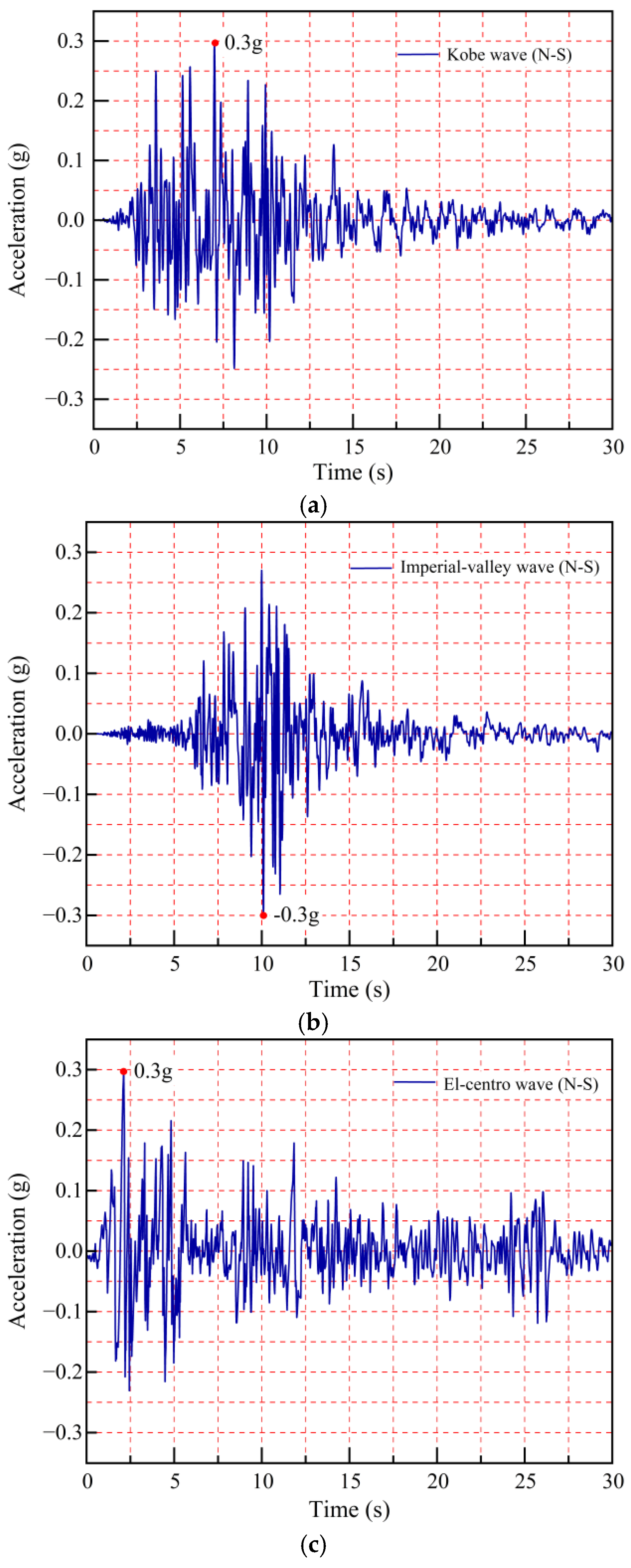
To account for the group anchor effect, an additional anchor 2 was introduced at a height of 8 m on top of the slope for further analysis. The impacts on the anchor rod force, dynamic yield acceleration, and seismic permanent displacement of the slope were thoroughly investigated. The original anchor was named anchor 1. Three distinct seismic records—the Kobe, El-Centro, and Imperial Valley earthquakes (Figure 10)—were selected to evaluate the proposed method under diverse seismic scenarios. The selected seismic records represent surface-level ground motions rather than bedrock-level inputs, as they inherently incorporate site-specific amplification effects. According to the previous study [16,20,33], these motions were chosen from a comprehensive database of accelerograms based on their heterogeneous frequency contents and intensity measures (e.g., peak ground acceleration, PGA), ensuring a robust assessment of the method’s performance across varying ground motion characteristics. To facilitate the comparative analysis, the PGA values of all records were normalized to 0.3 g, and the duration of each seismic time history was truncated to 30 s. To better understand the frequency characteristics of the seismic waves used in this study, a Fourier transformation analysis was conducted. The acceleration–time curves for these seismic waves are shown in Figure 11. The predominant frequencies of the El-Centro, Kobe, and Imperial Valley waves were found to be 2.5 Hz, 0.8 Hz, and 2.0 Hz, respectively. These predominant frequencies are consistent with those reported in previous studies [10,34,35,36] and provide valuable insights into the dynamic response of the anchored slopes under seismic loading. Consequently, the ratio of vertical seismic acceleration to horizontal seismic acceleration ($\lambda$) was varied, set to 0, 1/3, and 2/3.

4.1. Anchor Force

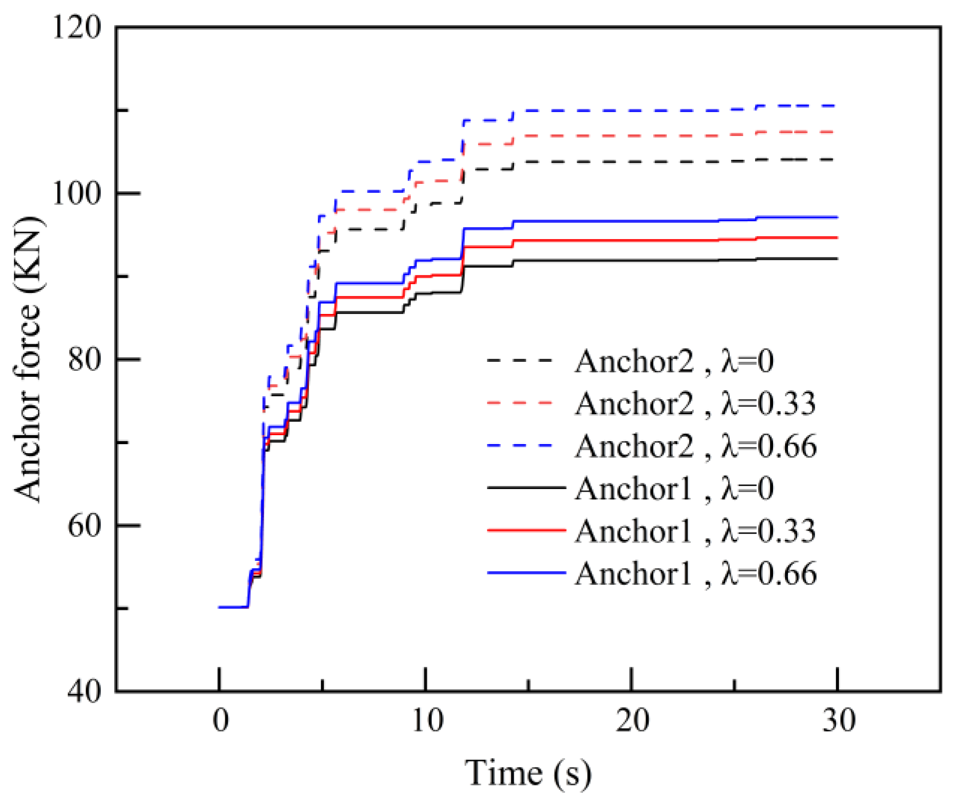
Figure 12 depicts the variation in anchor rod forces at different heights over time under the El-Centro seismic wave with varying ratios of $\lambda$, utilizing the AMNB method. During seismic activity, the slope experiences displacement, resulting in the elongation of the anchor rod. Consequently, the anchor rod force continuously increases with slope displacement, effectively restraining further slope deformation.

The initial pre-stress for both Anchor 1 and Anchor 2 is 50 kN. From the graph, it can be observed that when $\lambda$ is 0, 0.33, and 0.66, the maximum axial force on Anchor 1 increases to 92.1 kN, 94.6 kN, and 97.1 kN during the seismic event. Similarly, for Anchor 2, the maximum axial force rises to 104.1 kN, 107.4 kN, and 110.6 kN. These data highlight the significant influence of vertical seismic motion on the maximum axial force of anchor rods supporting the slope. For example, with λ = 0, both Anchor 1 and Anchor 2 exhibit a similar increasing trend under seismic action, with growth rates of 84.2% and 108.2%, respectively. This indicates that the axial force in the lower anchor rod increases more rapidly than the upper anchor rod. The lower anchor rod at the bottom of the slope bears a greater tensile force during the seismic process, which aligns with findings from previous studies [8,37,38].

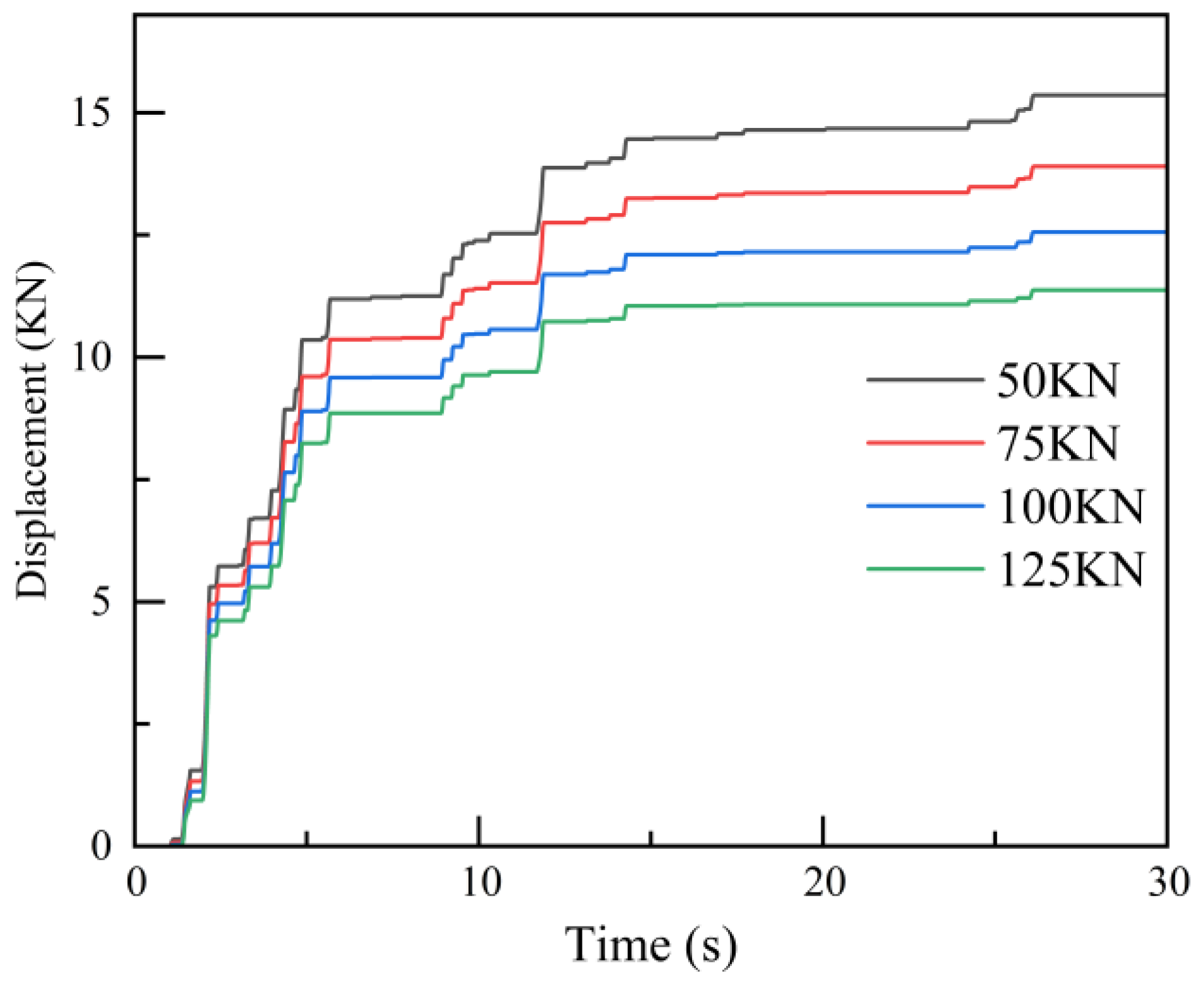
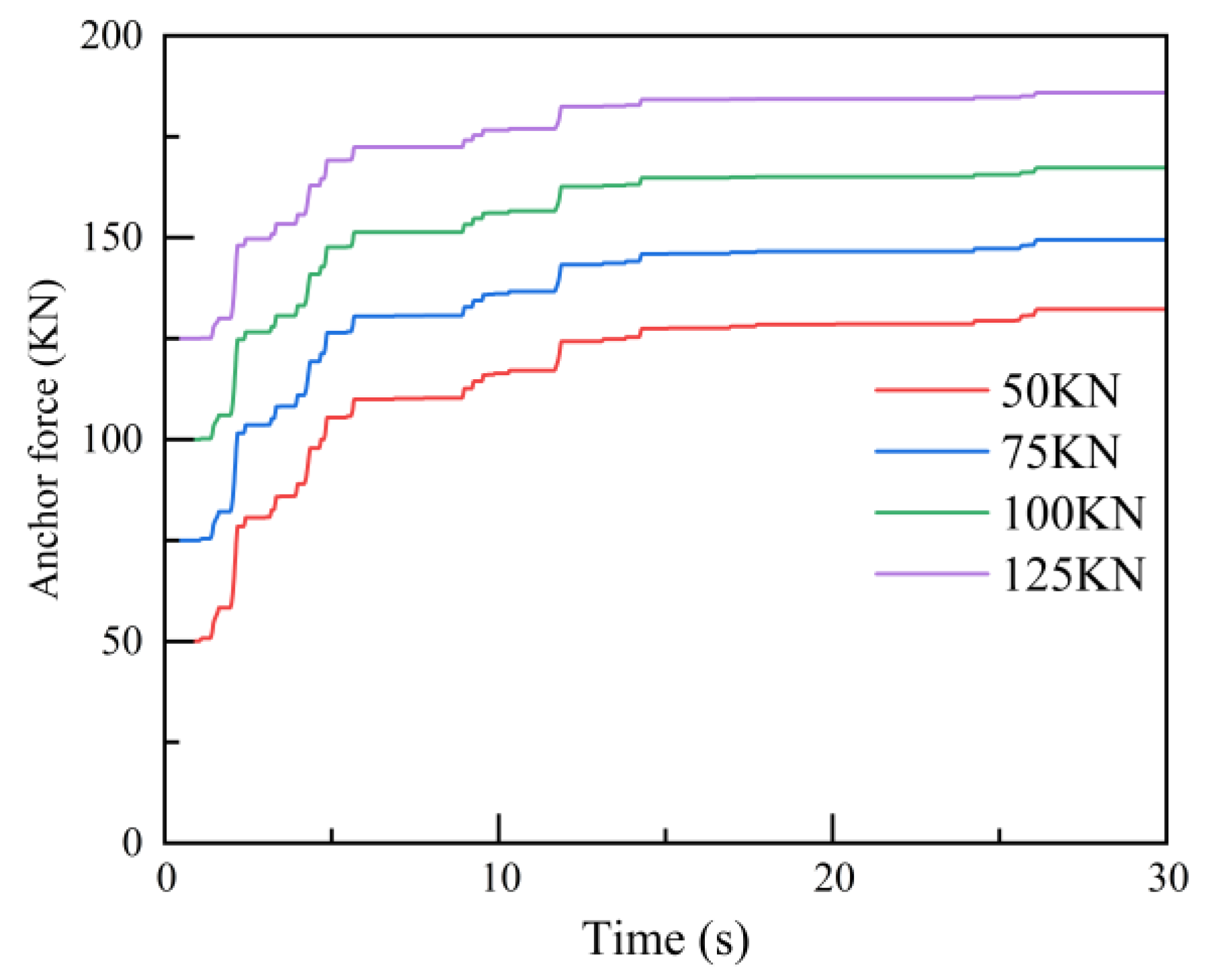
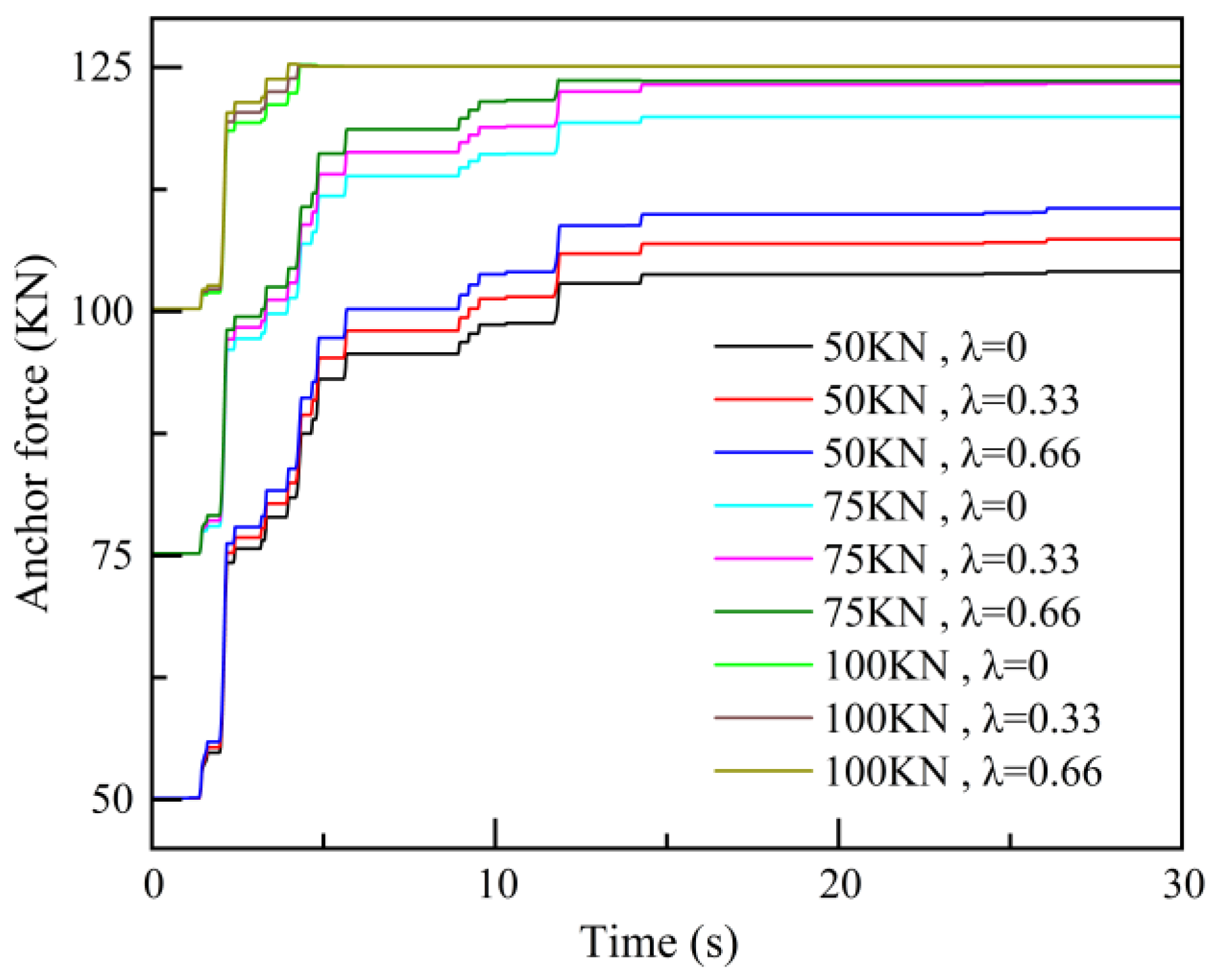
Figure 13 shows the variation in anchor axial forces under the influence of the El-Centro earthquake wave for different initial pre-stresses in Anchor 2. When the initial pre-stress is 50 KN, the axial force of the anchor continuously increases during the seismic process, peaking at 26.1 s. On the other hand, when the initial pre-stress is 100 KN, the axial force reaches its peak at 4.4 s. This difference arises because, with an initial pre-stress of 50 kN, the axial force continues to rise throughout the seismic process but does not reach the maximum pull-out force of the anchor by the end of the earthquake. Conversely, with an initial pre-stress of 100 kN, the axial force reaches the maximum pull-out capacity during the seismic event, and thereafter, the axial force remains constant. 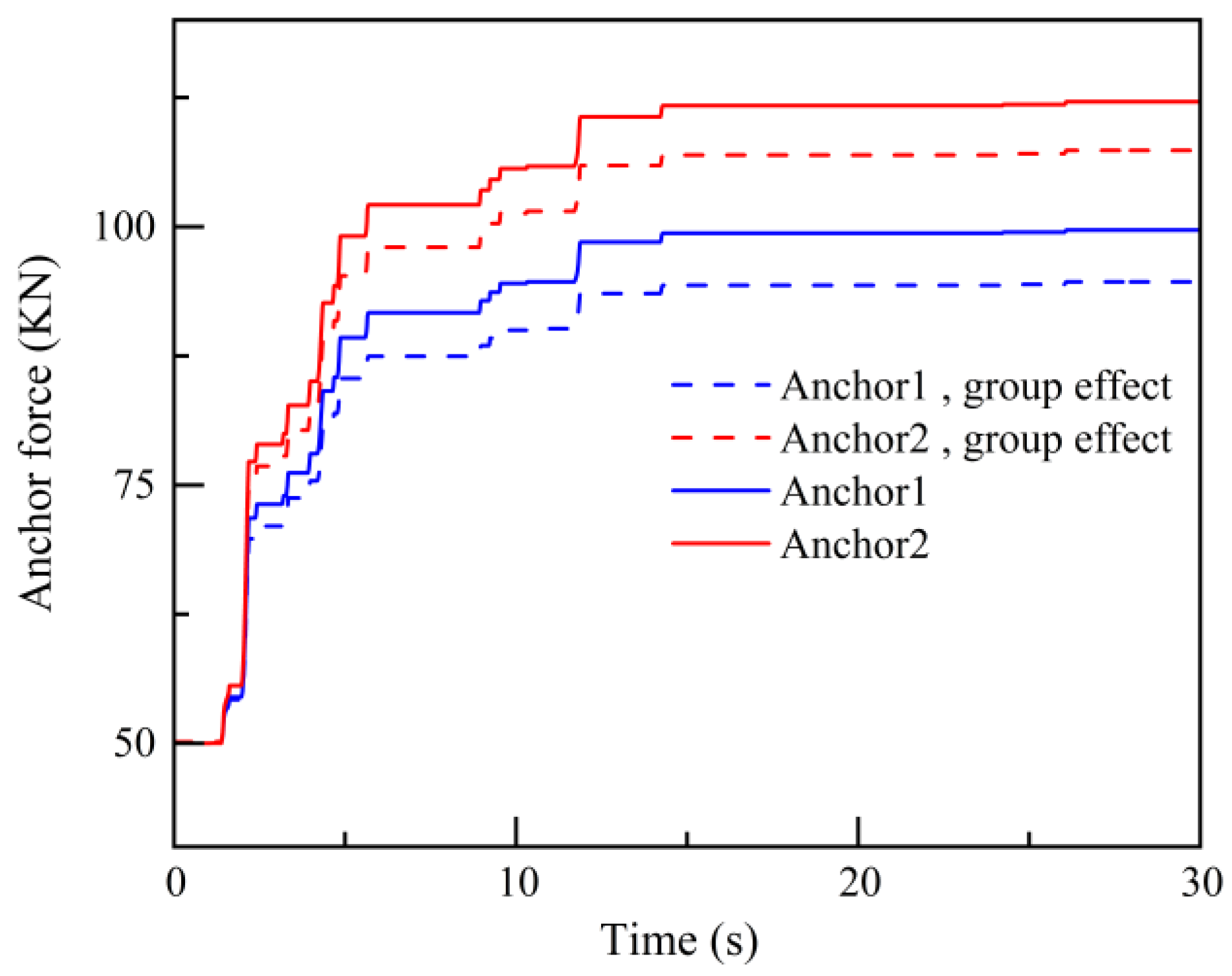Figure 14 illustrates the influence of group anchor effects on the variation in anchor rod axial forces when λ = 0.33. From the graph, it can be observed that the maximum anchoring forces in Anchor 1 and Anchor 2 decrease by 5.1% and 4.6%, respectively, due to the impact of group anchor effects. This indicates that group anchor effects are significant and should not be overlooked in the stability analysis of slopes. These findings demonstrate that neglecting the influence of the maximum axial force and group effect on anchor bolts in slope stability results in non-conservative stability assessments, potentially compromising the safety of practical engineering projects.

4.2. Dynamical Yield Acceleration

In the traditional NSBM, the yield acceleration remains constant throughout the calculation process. However, as discussed in the previous section, during a seismic event, the axial force in the anchor changes continuously over time and with slope displacement. Therefore, for an anchor-supported slope, the yield acceleration is not static; it varies with time and is referred to as the dynamic yield acceleration.

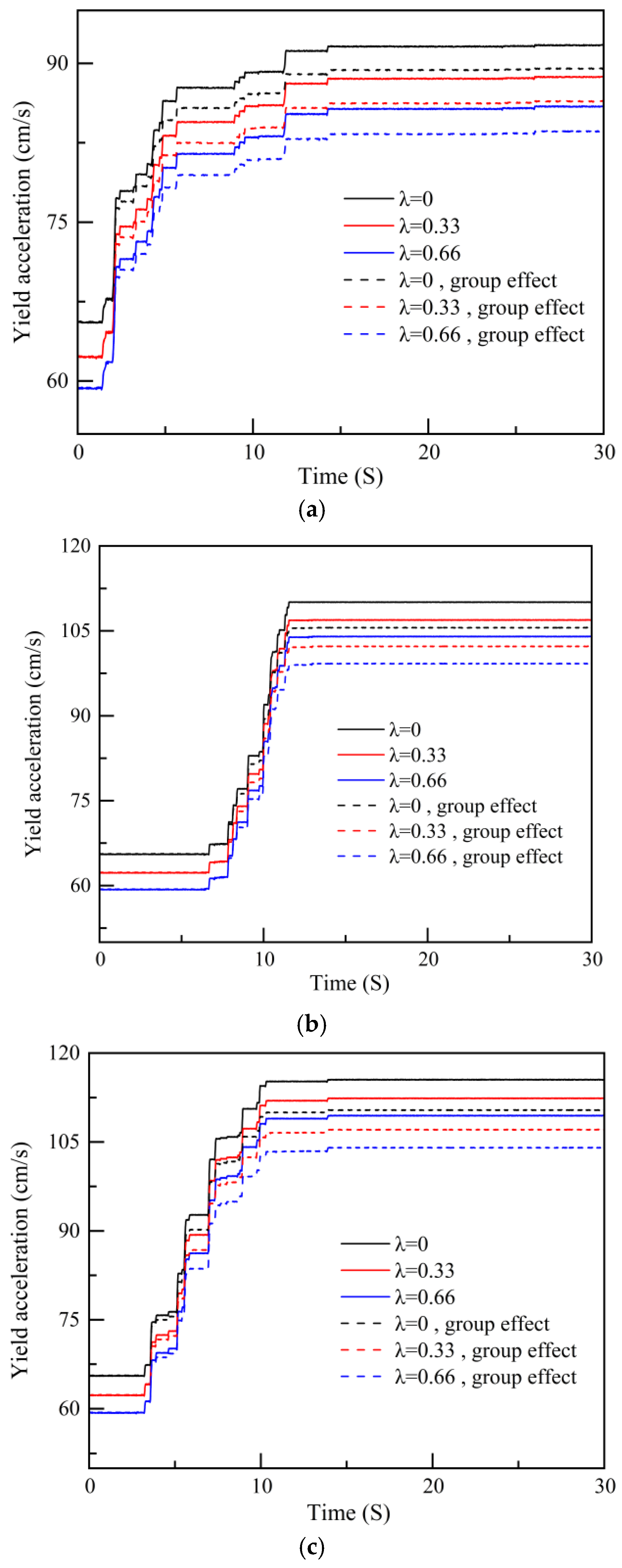
Figure 15 illustrates the dynamic yield acceleration of a slope reinforced by pre-stressed anchors under different seismic ground motions. During the excitation of seismic ground motion, the dynamic yield acceleration continuously increases. For example, when $\lambda$ = 0.33 and considering the group anchor effect, the dynamic yield acceleration increased by 37.5%, 39.3%, and 44.2% during the processes of El-Centro, Imperial Valley, and Kobe seismic motions, respectively. The graph reveals that the trends and magnitudes of dynamic yield acceleration vary with different seismic waves. Under the El-Centro seismic motion, the dynamic yield acceleration increases rapidly from 2 to 15 s. For the Imperial Valley seismic motion, a rapid increase in dynamic yield acceleration is observed from 7 to 11 s. In the case of the Kobe seismic motion, the dynamic yield acceleration increases significantly from 3 to 11 s. To verify the validity of the predicted yield acceleration, a comparison between yield acceleration and input base acceleration is presented in Figure 16. The input base acceleration exceeding the yield acceleration is defined as the effective acceleration required for calculating seismic displacement. The results indicate that the occurrence time of effective acceleration coincides with the growth period of yield acceleration, which is consistent with the pattern observed in Figure 15, indirectly corroborating the accuracy of the calculation results. This increase is attributed to the sustained augmentation in anchor rod axial force throughout the seismic event. When the base acceleration exceeds the yield acceleration, slope displacement occurs, causing anchor elongation and increased axial force, which in turn leads to an increase in yield acceleration. This dynamic interplay underscores the crucial role of anchor support in augmenting slope stability under seismic conditions.

From the graph, it can be observed that when considering group anchor effects, the dynamic yield accelerations for each scenario are reduced to varying degrees. Taking $\lambda$ = 0.33 as an example, when considering group anchor effects, the maximum dynamic yield accelerations under El-Centro, Imperial Valley, and Kobe seismic motions are 85.81 cm/s², 106.51 cm/s², and 106.92 cm/s², respectively. Without considering group anchor effects, the maximum dynamic yield accelerations are 88.71 cm/s², 112.41 cm/s², and 101.62 cm/s², respectively. As a result, the maximum dynamic yield accelerations are reduced by 3.2%, 5.2%, and 4.9% under the respective seismic motions when group anchor effects are considered. This reduction is unfavorable for slope stability, the lower yield acceleration means that the slope will produce greater displacement during the earthquake, highlighting the importance of considering group anchor effects when evaluating the stability of supported slopes.

Additionally, it can be observed from the graph that vertical seismic acceleration significantly impacts the magnitude of dynamic yield acceleration. When considering group anchor effects, the maximum dynamic yield accelerations under El-Centro seismic motion for $\lambda$ values of 0, 0.33, and 0.66 are 88.8 cm/s², 85.8 cm/s², and 83.0 cm/s², respectively. Similarly, under Imperial Valley seismic motion, the values are 59.9 cm/s², 63.1 cm/s², and 66.0 cm/s², and under Kobe seismic motion, the values are 67.2 cm/s², 70.9 cm/s², and 74.1 cm/s². Therefore, the presence of vertical seismic acceleration is detrimental to slope stability, and as λ increases, the slope yield acceleration decreases. Hence, the influence of vertical seismic acceleration on slope stability should not be ignored in design, consistent with previous research findings [10]. In summary, the presence of anchor rod support enhances the dynamic yield acceleration of the slope; the existence of group anchor effects and vertical seismic acceleration results in a reduction in the slope yield acceleration, adversely affecting slope stability.

4.3. Seismic Permanent Displacement

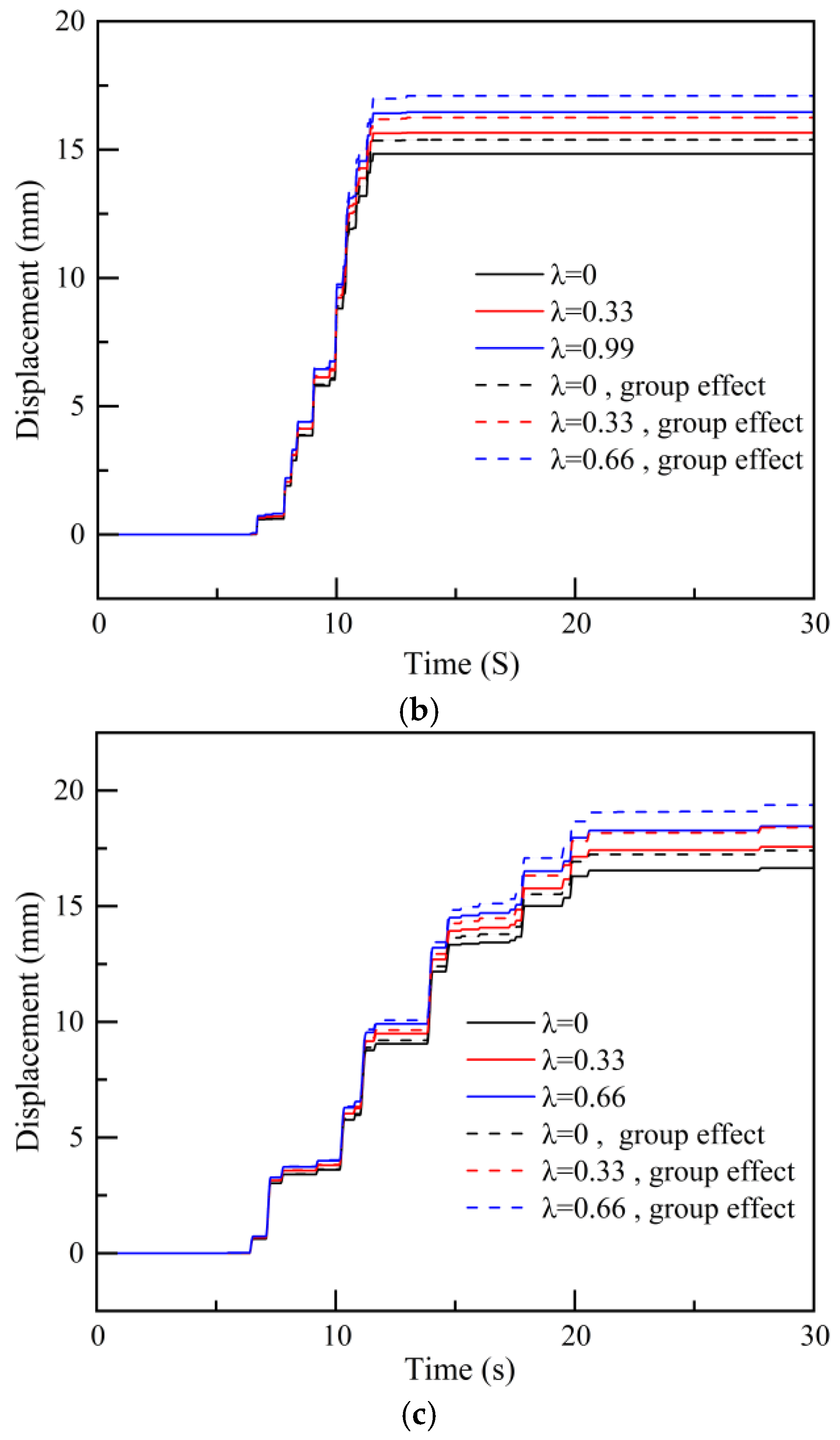
Figure 17 illustrates the seismic permanent displacement of the slope reinforced by pre-stressed anchors under different ground motions. Despite having the same peak acceleration and seismic duration for each seismic motion, the seismic permanent displacement of the slope varies significantly under different seismic actions. Taking $\lambda$ = 0.33 as an example, considering group anchor effects, the maximum displacement under Kobe seismic action is 18.6 mm, followed by 16.2 mm under Imperial Valley seismic action, and the minimum is 9.63 mm under El-Centro wave action.

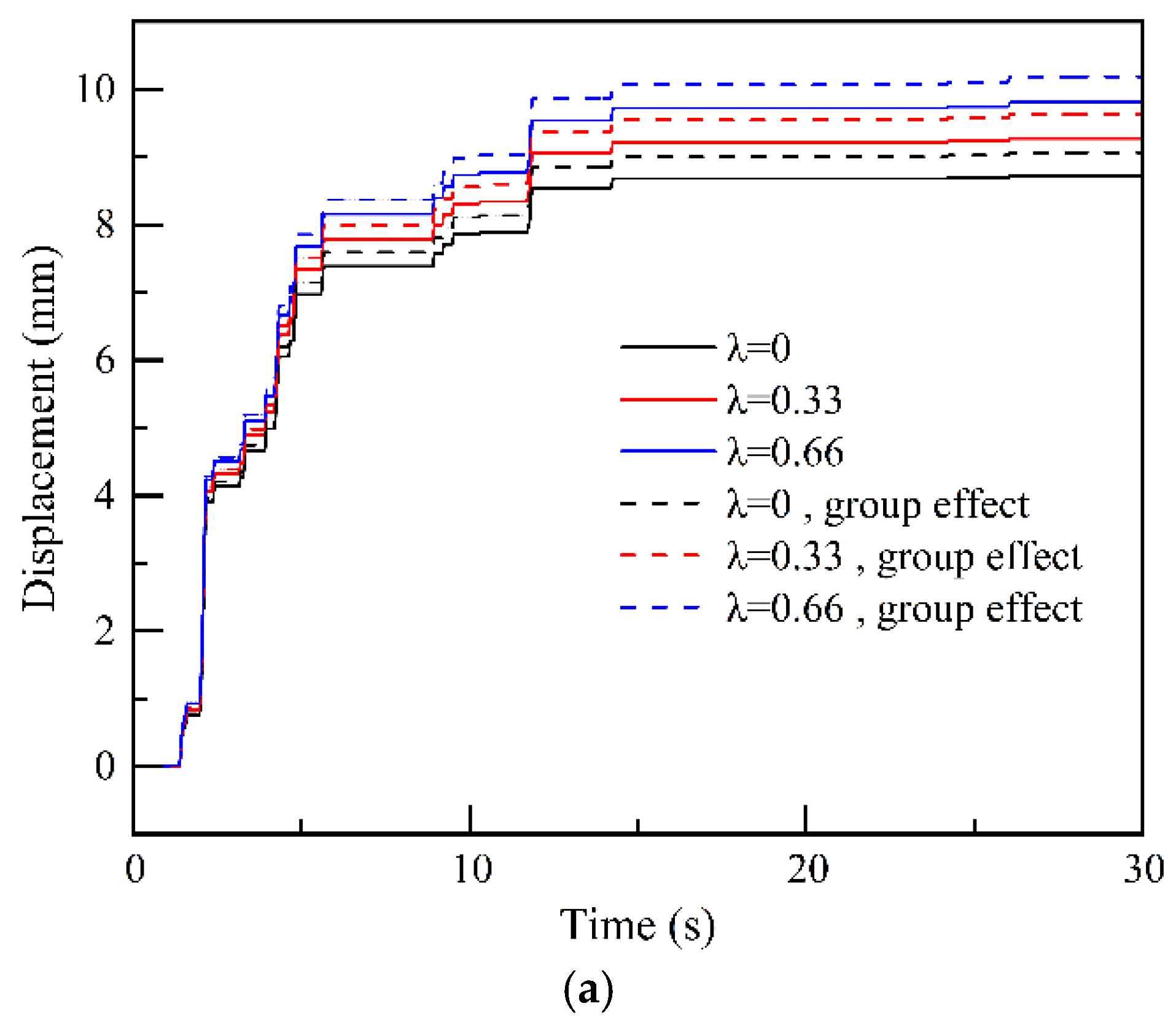
From the figure, it is also evident that the horizontal seismic permanent displacement is related to the duration of seismic motion, and the seismic permanent displacement of the slope is 5~10% larger when considering group anchor effects. Using $\lambda$ = 0.33 as an example, under El-Centro, Kobe, and Imperial Valley seismic actions, considering group anchor effects increases the slope’s seismic permanent displacement by 0.3 mm, 1.1 mm, and 0.6 mm, respectively. This also indicates that the presence of group anchor effects is detrimental to the stability of the slope supported by anchor rods. Similarly, the presence of vertical seismic acceleration increases the seismic permanent displacement of the slope. For instance, when considering group anchor effects under El-Centro seismic motion, the seismic permanent displacement increases by 0.56 mm and 1.11 mm for $\lambda$ = 0.33 and 0.66, respectively, compared to $\lambda$ = 0.

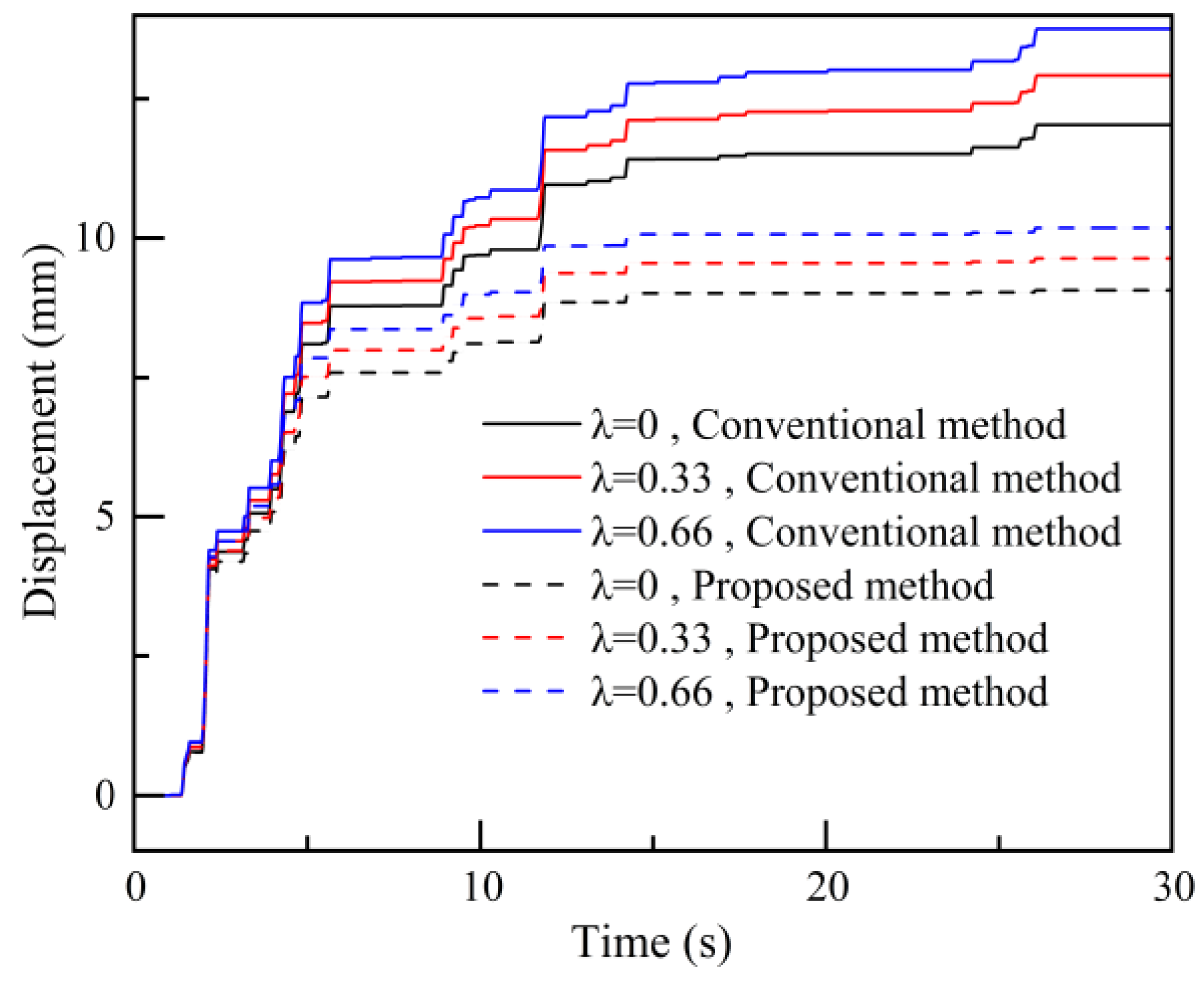
Additionally, to investigate the impact of dynamic yield acceleration on the slope’s permanent displacement, Figure 18 compares the horizontal seismic permanent displacement results determined by the proposed method and the conventional method under the El-Centro seismic action. In the conventional method, a constant yield acceleration is used to calculate the horizontal seismic permanent displacement, with fixed values of 65.6 cm/s², 62.3 cm/s², and 11.446 cm/s² for $\lambda$= 0, 0.33, and 0.66, respectively. In contrast, under the same conditions, the maximum dynamic yield acceleration determined by the anchor rod force-corrected Newmark method is 92.1 cm/s² (refer to Figure 16a). It is evident that the horizontal seismic permanent displacement determined using the dynamic yield acceleration method is significantly smaller than that calculated by the conventional method. For instance, at $\lambda$ = 0, the final slope’s seismic permanent displacement calculated by the anchor rod force-corrected method is 9.1 mm, while the conventional method calculates a final slope’s seismic permanent displacement of 12.1 mm. This indicates that the substantial increase in dynamic yield acceleration during the seismic process, due to anchor rod forces, significantly reduces the slope’s seismic permanent displacement. Consequently, this suggests that the traditional NSBM is conservative when calculating the displacement of bolt-supported slopes.

4.4. Group Anchor Effect Coefficient

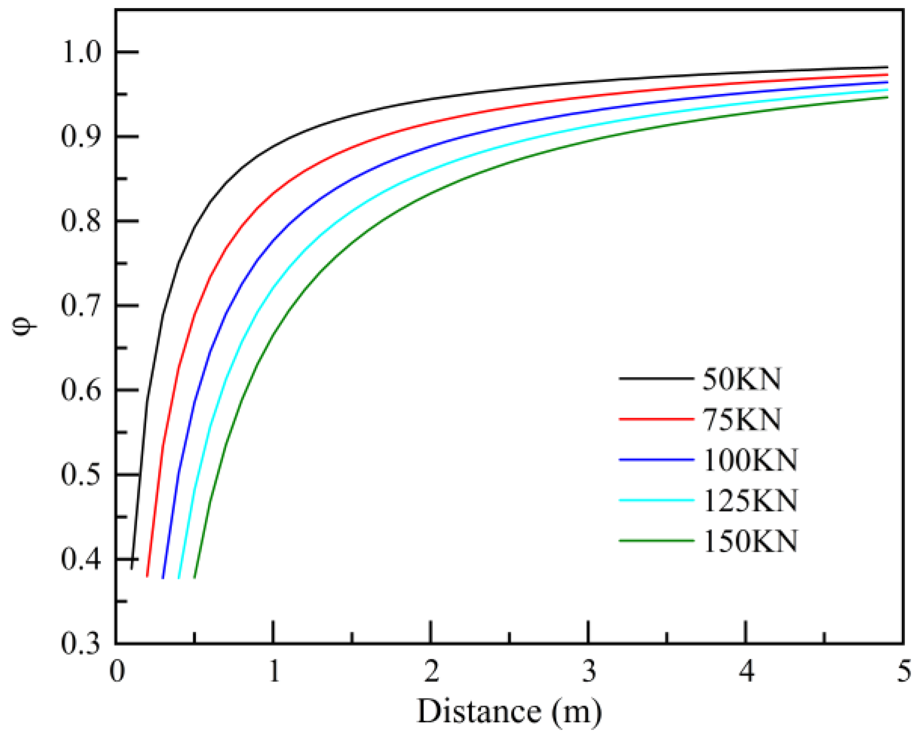
According to the conclusions drawn from the Mindlin solution theory, the group anchor effect coefficient can be calculated for different anchor spacings and anchor pre-stressed forces. Figure 19 illustrates the variation in the group anchor effect coefficient for an anchor rod with a force of 50 KN, considering different forces and spacings for surrounding single anchors.

From the figure, it is evident that the group anchor effect coefficient is significantly influenced by anchor spacing. When the spacing exceeds 3 m, the group anchor effect coefficient approaches 1, indicating that the effect is minimal. In contrast, the coefficient rapidly decreases when the spacing is less than 1.5 m. This suggests that at spacings greater than 3 m, the group anchor effect is not pronounced, and the anchor rod force is only slightly affected by the surrounding anchors. However, within a spacing of 3 m, the group anchor effect becomes significant, with the anchor rod force being substantially influenced by the forces from neighboring anchors. When the spacing is less than 1.5 m, the anchor rod is heavily impacted by the group anchor effect, potentially leading to a rapid decrease in anchor rod force and posing a significant risk.

The graph also indicates that the group anchor effect coefficient is significantly influenced by the surrounding anchor rod forces. For example, at a spacing of 2 m, the group anchor effect coefficients for surrounding anchor rod forces of 50 kN, 75 kN, 100 kN, 125 kN, and 150 kN are 0.94, 0.92, 0.89, 0.86, and 0.83, respectively. This demonstrates that as the surrounding anchor rod forces vary, the axial force of the central anchor rod decreases by 6% to 13%. As mentioned earlier, the anchor rod force increases continuously during the seismic process, leading to a corresponding increase in the group anchor effect coefficient. Therefore, the group anchor effect is crucial in the analysis of slope stability and should be given adequate attention in the analytical process.

5. Discussion

The AMNB method represents a significant advancement in slope stability analysis, particularly for predicting seismic permanent displacements in anchored slopes. Traditional methods often fail to account for factors such as group anchor effects and dynamic tension changes, which the AMNB method incorporates to offer more accurate predictions of slope behavior. This improvement is essential for ensuring the safety and performance of slopes in seismic regions.

Despite these benefits, the AMNB method has limitations. It assumes homogeneous soil conditions and linear elastic anchor behavior, simplifying real-world scenarios. In practice, materials often exhibit non-linear behavior, geological formations are often heterogeneous, and the simplification of homogeneity and linear elastic anchor behavior could affect the accuracy of predictions related to anchor forces and displacement. Future research should focus on incorporating the non-linear behavior of anchors, the heterogeneity of slope materials, and anchor–soil interaction under large deformations into the analysis. This would improve prediction accuracy and offer a more comprehensive understanding of system behavior.

The method also simplifies seismic loading into horizontal and vertical components, neglecting the effects of rotational or shear forces, which can have significant impacts on slope behavior during seismic events. These simplifications, while balancing efficiency and accuracy, limit the model’s ability to fully replicate real-world conditions. Future work should focus on incorporating more complex, non-homogeneous material models to better capture the variability of soil and rock masses, improving prediction accuracy.

While the current study introduces a group anchor effect coefficient to address interactions between closely spaced anchors, it does not fully capture the local stress redistribution that occurs in these configurations. Incorporating stress redistribution would increase the model’s complexity, requiring advanced 3D numerical simulations or finite element modeling. Furthermore, integrating detailed 3D analysis and local stress redistribution effects would improve the precision of anchor force predictions and displacement estimates in closely spaced configurations, though this would increase model complexity.

Another limitation is that the model does not account for long-term degradation factors, such as the corrosion, creep, or relaxation of pre-stressed anchors. These factors are crucial for assessing the long-term stability and performance of reinforced slopes, especially in aging infrastructure. As the current model focuses primarily on the immediate seismic response, it overlooks the gradual changes in anchor behavior caused by environmental and material degradation. Future research should incorporate time-dependent material models to account for these degradation mechanisms. This would provide a more realistic assessment of slope stability over the lifespan of reinforcement and improve the method’s applicability in long-term engineering scenarios.

6. Conclusions

This study presents an AMNB method for calculating seismic permanent displacement in anchored slopes, incorporating critical factors such as maximum anchor rod tension and group anchor effects. Based on Mindlin’s solution in elastic mechanics, the method formulates the calculation of maximum anchor rod tension and the group anchor effect coefficient. A case study of a typical reinforced slope was conducted to validate the AMNB method, with results compared to existing methods and numerical simulations. The key findings and conclusions are as follows:

• The AMNB method significantly improves the traditional NSBM approach by integrating group anchor effects and maximum axial force considerations. It quantifies the influence of overlapping shear stress fields on anchor group capacity, highlighting that anchor spacing below 3 m significantly reduces individual anchor forces due to group effects. Additionally, the method demonstrates that axial forces may reach their maximum pull-out capacity during seismic events, compromising slope stability. Neglecting these effects can lead to non-conservative stability assessments, posing risks to engineering safety.
• By accounting for dynamic changes in anchor tension and group anchor interactions, the AMNB method provides seismic permanent displacement predictions that align more closely with numerical simulations, typically yielding 5–10% smaller displacements. This validates the method’s effectiveness in delivering more accurate stability assessments for anchored slopes during seismic events, improving the reliability of seismic stability predictions.
• The study also reveals that different seismic waveforms significantly affect dynamic yield acceleration and permanent displacement. Vertical seismic acceleration was found to reduce yield acceleration by up to 5% and increase permanent displacement by 10%, negatively impacting slope stability. These findings emphasize the importance of including vertical seismic effects in the design and analysis of anchored slopes to ensure more accurate safety assessments.

This method provides several practical advantages for engineers and researchers working with slope stabilization in seismic areas. By incorporating dynamic anchor behavior, it accounts for group anchor effects and variations in anchor tension during seismic events. This enables more informed design choices, and improving efficiency while reducing material costs. This capability is particularly useful for assessing the performance of secondary reinforcements in aging infrastructure. Although the AMNB method shows significant promise, future work should focus on incorporating non-linear behavior, heterogeneous materials, and multi-directional seismic forces for improved accuracy and a more comprehensive understanding of slope dynamics.