Uncertainty and Prediction Intervals of New Machine Learning Approach for Non-Destructive Evaluation of Concrete Compressive Strength

Abstract

This paper presents a machine learning (ML) model for predicting concrete strength using a combination of two non-destructive testing (NDT) methods: ultrasonic pulse velocity (UPV) and rebound number (RN). The model was developed using an extensive and diverse dataset and is the first such model to consider the effect of three different sample types: cubic, cylindrical, and core samples. This study is also the first of its kind to present an in-depth analysis of the results to quantify model uncertainty, which is an important prerequisite for its use in practice. Accordingly, two ML models were trained using 620 data points from the aforementioned sample types. The prediction intervals and associated uncertainties of the ML-based approach were thoroughly examined. Validation with the testing dataset showed that 93% of the testing data points for the combined cylindrical and cubic dataset fell within the 95% prediction interval, indicating strong alignment with expected results. Based on the findings, a roadmap is also proposed for future work.

1. Introduction

In the evaluation of concrete infrastructure, the most important mechanical parameter is the compressive strength (CS) of the concrete [1,2], whether in structures under construction or those already built. For structures under construction, the CS of the concrete is measured on cylindrical or cubic samples taken from fresh concrete during pouring. However, for reinforced concrete (RC) structures that were built many years ago, other means of determining concrete CS are required. Structures being considered for structural health monitoring, rehabilitation or repair, or detailed condition assessments first require engineers to find ways to assess the CS of the concrete. Usually, the most prominent option for engineers is drilling and extracting cores followed by compressive tests on the cores, which are known as a “core test” or “destructive test (DT)”.

In recent years, due to issues associated with core tests, such as safety considerations, high costs, limitations of access, and repeatability, engineers and researchers have sought alternative approaches [3]. One method that has attracted engineers’ attention is non-destructive testing (NDT) of concrete [4,5,6]. In this method, tests are conducted using devices that do not damage the concrete, and the results are usually used to indirectly estimate the CS of the concrete [7]. Two such tests are the rebound number (RN) test, conducted with a Schmidt hammer, and the ultrasonic pulse velocity (UPV) test, conducted with a UPV device. The combined use of these two NDT methods is known as the “SONREB method” [8].

To convert the results of SONREB to CS, there are a number of traditional empirical equations (traditional approach) used. However, according to previous research [3,9,10,11,12], these traditional empirical equations are typically based on specific datasets, which often represent a limited range of concrete types or conditions. These equations are not necessarily applicable to a wider variety of concrete mixes or environmental factors [12,13]. In contrast, ML models are trained on much larger and more diverse datasets, allowing for them to capture more complex, non-linear relationships between input variables and CS. This is one of the main reasons why, in recent years, machine learning (ML) and artificial intelligence (AI) have attracted the attention of engineers and researchers [9].

Over the past two decades, alongside advancements in AI and its most important method of ML, researchers have also been drawn to providing ML-based engineering solutions in the construction and civil engineering industry. Based on previous studies that reviewed the application of AI and ML in civil and structural engineering, a significant increase in research in this field has been observed in recent years [14,15,16,17]. Most of these studies focus on predicting the mechanical properties of concrete, including compressive strength.

One such topic is predicting the CS of concrete based on the results of the SONREB method. By investigating the reviewed papers on predicting concrete strength using ML/AI methods, it becomes clear that among all the studied scenarios (e.g., predicting concrete strength based on mix design, age, type of cement, etc.), relatively few studies have exclusively used data obtained from SONREB testing [14,15,18,19], despite the fact that in many cases, detailed mix design information is unavailable. The use of multiple parameters in a prediction model is understandable when trying to achieve the highest possible accuracy; however, it is worth considering that 1) such an approach makes complex models impractical for many real applications due to the lack of available data, and 2) engineers are accustomed to a certain degree of uncertainty when it comes to concrete CS (since even cylinder test results are characterized by considerable scatter) and in many cases, a good approximation may be sufficient provided that the uncertainty can be quantified. Given the simplicity and accessibility of the SONREB method, it is therefore interesting to consider the limits of its predictive ability when paired with advanced tools such as ML.

Na et al. conducted the first study that utilized a neuro-fuzzy system to improve result accuracy [20]. Subsequently, several other researchers have applied ANNs to estimate CS [21,22,23,24,25]. Demir applied ANNs for hybrid fiber-added concrete to predict CS, while Almasaeid et al. applied ANNs to the CS of geopolymer concrete [26,27]. Additionally, Almasaeid et al. used ANNs for the assessment of high-temperature damaged concrete [28]. Kumar and Kumar used genetic programming, while Shih et al. and Sai and Singh employed support vector machines (SVMs) to enhance result accuracy [29,30,31]. Poorarbabi et al. combined ANNs with response surface methodology for better predictions of CS [32]. Du et al. integrated GA-BP neural networks for high-performance self-compacting concrete, while Thapa et al. developed models for concrete with recycled brick aggregates [33,34]. Ngo et al., Shishegaran et al., Arora et al., Ramadevi et al., Erdal et al., and Asteris et al. discussed AI and soft computing advancements [35,36,37,38,39,40]. Park et al. used ML to extract new equations to convert the results of UPV and RN to CS [41]. Alavi et al. developed the first graphical user interface (GUI) app based on ML for on-site CS evaluations and then investigated its performance on case studies [3,11]. Additionally, Alavi and Noel applied ML and deep learning (DL) to propose a model that could work for both cylindrical and cubic strength standards [9,10].

Collectively, these previous studies provide a better understanding of how to develop and apply ML-based approaches for concrete CS predictions. However, before such an approach can be confidently applied in practice, it is essential that tools be developed to evaluate model performance and quantify the uncertainty that is inherent in any prediction method.

Therefore, the main objective of this study is to investigate, for the first time, the uncertainty in concrete strength prediction through a comprehensive analysis of new ML-based approaches in evaluating the CS of concrete without applying a calibration procedure (which requires core tests).

This study also introduces the first machine learning-based model that accounts for the differences between cubic, cylindrical, and core specimens and their effects on CS, while also discussing the remaining challenges. A roadmap for future model development is provided to address these challenges and help develop a universal ML model based on the SONREB method for CS prediction in future. The results show that ML could improve the accuracy and reliability of concrete strength prediction and provide better results compared to traditional mathematical models at this stage with the available data, despite the challenges that remain.

2. SONREB

The SONREB method combines two NDT techniques, UPV and RN, used for CS evaluation in existing RC structures to provide more reliable estimates than either method on their own [12,42] as shown in Figure 1. The UPV device measures the transmission time ($t$) of an ultrasonic pulse that passes through the concrete between the transmitter and receiver. By dividing the distance between transmitter and receiver ($l$) by the transmission time ($t$) the pulse velocity ($V$) will be obtained. The RN test is performed at the same location using the rebound hammer (also known as the Schmidt hammer), a simple mechanical tool that releases a spring-loaded mass that strikes the target surface of the concrete with a defined force (based on the type and manufacturer). ASTM C805 [43] requires ten readings at each location and the average is considered the final RN.

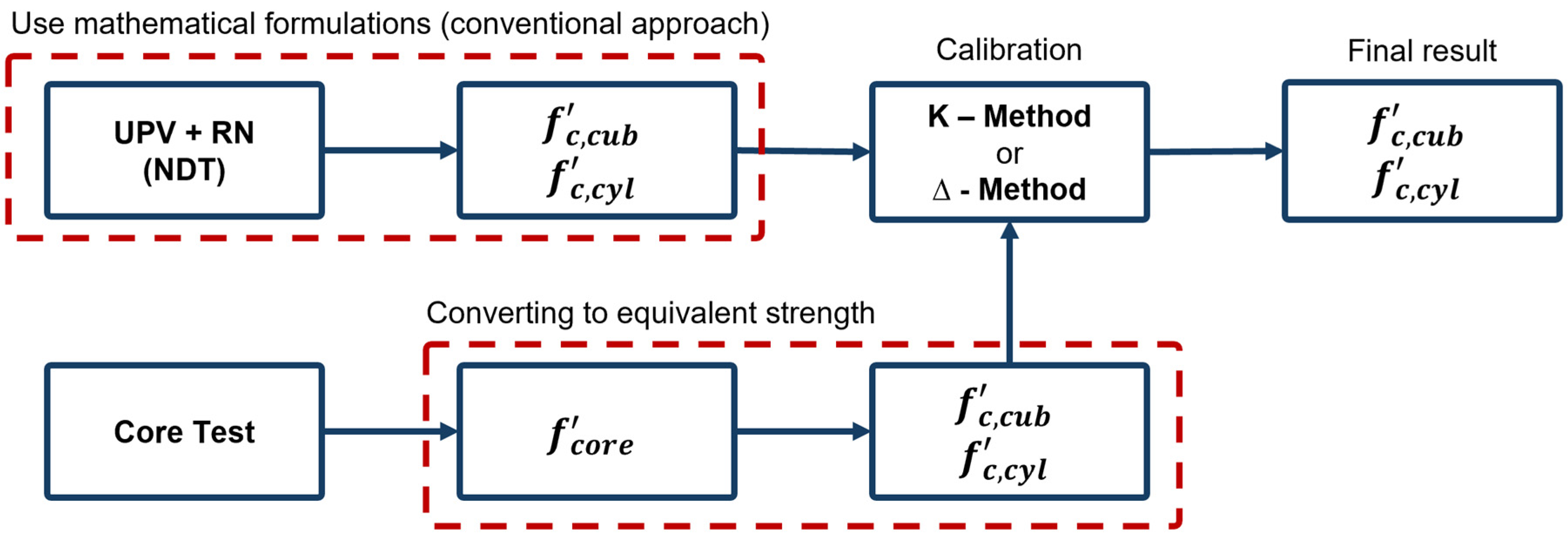
Based on the SONREB method, many models or equations have been proposed to predict the CS of concrete [11,12,44]. These models can be divided into two general categories. The conventional approach is to use regression analysis to develop empirical equations, while more recently ML-based models have been proposed [3]. The main difference between conventional regression analysis and ML-based models lies in the calibration process. The former relies on closed-form mathematical relationships with a specified form that are “fitted” with experimental data. As shown in Figure 2, current code provisions [3,11], allow for engineers to use results from these mathematical relationships following a calibration process using core data from a particular structure. Two general methods are used for calibration, which are the shifting factor method (D-method) and the multiplying factor method (K-method), to adjust model outputs with site-specific data [45,46,47]. The calibrated model can then be used to evaluate concrete CS based on NDT results at other points of the structure. While the number of cores required may be potentially reduced through the use of this NDT-based approach, the aforementioned challenges associated with core extraction remain. It should also be noted that due to safety concerns and other issues related to coring, the required core size has decreased in codes and guidelines in recent years (diameter less than 100 mm) [3]. Therefore, it is necessary to convert the CS obtained from tests on cores into equivalent cylinder or cube CS with standard sizes, depending on the applicable standard [48]. Numerous mathematical relationships have been proposed to convert SONREB to CS in recent decades [12,13]. In

Table 1. Selected formulations for converting SONREB to CS.

ID	Formulation	Unit	Ref.
Equation (1)	$f_{c,cyl}^{\prime }=-24.1+1.24\times \left(RN\right)+0.058\times \left({UPV}^4\right)$	MPa, km/s	[49]
Equation (2)	$f_{c,cyl}^{\prime }=-12+0.76\times \left(RN\right)+0.1\times \left({UPV}^4\right)$	MPa, km/s	[50]
Equation (3)	$f_{c,cyl}^{\prime }=-39.57+1.532\times \left(RN\right)+5.0614\times \left(UPV\right)$	MPa, km/s	[51]
Equation (4)	$f_{c,cyl}^{\prime }=5.9+2.712\times {10}^{-15}\times \left(RN\right)\times \left({UPV}^4\right)$	MPa, m/s	[52]
Equation (5)	$f_{c,cub}^{\prime }=0.0286\times \left({RN}^{1.246}\right)\times \left({UPV}^{1.85}\right)$	MPa, km/s	[53]
Equation (6)	$f_{c,cub}^{\prime }=0.0158\times \left({RN}^{1.1171}\right)\times \left({UPV}^{0.4254}\right)$	MPa, m/s	[54]
Equation (7)	$f_{c,cub}^{\prime }=2.6199\times {10}^{-8}\times \left({RN}^{0.5341}\right)\times \left({UPV}^{2.2878}\right)$	MPa, m/s	[55]
Equation (8)	$f_{c,cub}^{\prime }=0.26511\times \left(RN\right)+0.01385\times \left(UPV\right)-34.51583$	MPa, m/s	[55]

Note: $RN$: rebound number; $UPV$: pulse velocity; $f_{c,cyl}^{\prime }$: cylindrical strength; $f_{c,cub}^{\prime }$: cubic strength.

, eight well-known mathematical formulations are listed; Equations (1)–(4) are based on the cylinder standard ($f_{c,cyl}^{\prime }$) and Equations (5)–(8) are based on the cubic standard ($f_{c,cub}^{\prime }$).

The main goal of new ML-based approaches is to harness the power of computer models to minimize the need for calibration as much as possible. This approach is based on the premise that more complex ML models may be developed to potentially address the challenges faced with the conventional mathematical approach. However, as previously noted, available studies in this area are still limited and the reliability of this approach requires further investigation.

3. New ML-Based Approach

It can be said that machine learning (ML) is one of the most important subfields of artificial intelligence (AI). This method is used when humans cannot establish a relationship between inputs and outputs using a mathematical formula, or the problem might be so complex that this process would be time-consuming and costly. By using ML algorithms and raw data, computers can learn, find the relationships, and then provide a model that can be used for new inputs (this method is generally known as supervised machine learning, Figure 3).

As mentioned, numerous studies in recent years have focused on applying ML to the SONREB method, targeting various objectives. These studies frequently report statistical measures such as mean absolute percentage error (MAPE), correlation (R), and other performance indicators, which provide a useful overview of model accuracy. However, these metrics alone do not fully address the practical concerns of engineers, who must evaluate the risks associated with deploying these models in real-world scenarios without prior calibration. Specifically, there is a need to understand the probability that actual strength in specific parts of a structure may significantly deviate from the predicted values, along with the potential range of errors. These considerations are crucial for assessing the reliability of ML models in this context.

Recognizing this gap, the present study not only develops a comprehensive ML model based on a large dataset but also conducts a thorough reliability analysis to quantify the likelihood of error and the tolerance level between predicted and actual CS, providing a more detailed assessment of the risks associated with using ML-based approaches.

3.1. Data

The first step in developing any ML model based on the supervised method is creating a database. In this specific case, developing a model that can predict concrete CS is challenging, as sufficient and reliable data are limited [56]. However, through extensive review of past studies, a total of 620 data points were collected (

Table 2. Dataset information.

Dataset	ID	Ref.	Number	Geometry of Specimens	Detail
Training	No. 1	[57]	209	Cubic	-
	No. 2	[32]	56 *	Cubic	-
	No. 3	[58]	26	Cubic	-
	No. 4	[20]	20	Cubic	-
	No. 5	[59]	12	Cubic	-
	No. 6	[60]	39	Cubic	-
	No. 7	[61]	32	Cubic	-
	No. 8	[11]	8	Cylindrical	Company A ready-mix
	No. 9	[62]	60 *	Cylindrical	-
	No. 10	[10]	24 *	Cylindrical	Lab-prepared specimens
	No. 11	[22]	16	Core	-
	No. 12	[13]	69	Core	-
	No. 13	[11]	12 *	Core	RC slab
Testing	No. 14	[10]	12 *	Cylindrical	Company B ready-mix
	No. 15	[11]	8 *	Cylindrical	Lab-prepared specimens
	No. 16	[11]	8 *	Cubic	Lab-prepared specimens
	No. 17	[63]	9	Core	-

Note: (*) Each data point was extracted from the average results of three similar specimens.

). The database includes experimental data from the authors’ previous studies that were obtained from multiple sources as briefly noted in the ‘Detail’ section of Table 2. More information on those tests are reported elsewhere [10,11].

As shown in Table 2, seventeen different datasets were compiled to develop the ML model. The first thirteen datasets are considered as the training data, and the last four datasets (fourteen to seventeen) are used for testing. This approach for selecting training and testing data from distinct datasets is utilized according to the outcome of a previous study [11], which showed that using distinct data sources instead of randomly splitting the data into training and testing sets both reduces the bias between the testing and training data and increases the number of training data points. Figure 4 illustrates the distribution of data according to their geometry (core, cubic, and cylindrical).

Figure 5 shows the distribution of data according to three variables: UPV, RN, and CS. The upper graph plots UPV (Km/s) against CS (MPa), with blue points representing the training data and red points representing the testing data. The histograms show the frequency distribution of UPV and RN for both datasets, highlighting how the values are spread. The lower graph plots RN against CS (MPa), again with blue points for training data and red points for testing data. These visualizations are crucial for understanding the differences between the training and testing datasets, ensuring that the training data are adequate for training the model and that the testing data will be effective for evaluation. The training data shown in the two graphs are scattered over a wide range of 10 to 76 MPa, while the testing data range between 26 and 65 MPa. Additionally, the testing data are a good representation of the concrete typically used for structural purposes.

Table 3. Statistical features of NDT and DT variables.

Variable	Unit	Training			Testing
		Min	Max	Mean	Min	Max	Mean
UPV	Km/s	2.450	5.400	4.369	2.500	5.239	4.539
RN	-	10.33	55.50	30.05	24.07	50.90	38.96
CS	MPa	10.00	76.32	32.41	26.10	70.78	49.67

also provides more statistical information on the training and testing datasets.

3.2. ML Model Development

In this study, the adaptive neuro-fuzzy inference system (ANFIS) method was used following a comparison with other ML model types that is discussed elsewhere [10,36]. ANFIS is a single-output method, making it well suited for this study’s purpose. As shown in Figure 6, models based on the ANFIS method have a structure that includes five different layers [64], which is technically based on the feedforward neural network (NN) that merges fuzzy logic (FL) with neural networks [65,66,67]. Layer 1, the fuzzification layer, converts crisp input values into fuzzy membership values using membership functions. In this study, triangular membership functions were utilized. Layer 2, the fuzzy rule base layer, processes these values through fuzzy if–then rules to determine rule firing strengths. Layer 3, the inference engine layer, applies fuzzy logic operations to compute output fuzzy sets. Layer 4, the defuzzification layer, transforms these fuzzy sets into crisp output values. Finally, Layer 5, the output layer, produces the final ANFIS output, which in this case is a CS value (MPa). Each layer’s processing allows for the model to learn and adapt, optimizing fuzzy rules and membership functions during training for accurate predictions of CS.

Two ML models were developed using ANFIS and a dataset of 620 data points in MATLAB. Model No. 1 includes only two continuous numerical inputs, UPV and RN, to predict CS. In Model No. 2, two binary inputs were added to account for the differences between cylindrical, core, and cubic data. For the first and second inputs of both models (UPV and RN) and the output value (CS), which are continuous numerical variables, normalized values between 0.1 and 0.9 were used. Based on the minimum and maximum values of UPV, RN, and CS in Table 3, the actual data values were normalized to values between 0.1 and 0.9 according to the equations provided in

Table 4. Normalization equations for continuous numerical variables.

Variable	Unit	Equation
UPV	(km/s)	${\mathrm{U}\mathrm{P}\mathrm{V}}_{\mathrm{n}\mathrm{o}\mathrm{r}\mathrm{m}}=\left[(0.9-0.1)\times \left({\displaystyle \frac{\mathrm{U}\mathrm{P}\mathrm{V}-2.45}{2.95}}\right)\right]+0.1$	(Equation (9))
RN	--	${\mathrm{R}\mathrm{N}}_{\mathrm{n}\mathrm{o}\mathrm{r}\mathrm{m}}=\left[(0.9-0.1)\times \left({\displaystyle \frac{\mathrm{R}\mathrm{N}-10.33}{45.17}}\right)\right]+0.1$	(Equation (10))
CS	(MPa)	${\mathrm{C}\mathrm{S}}_{\mathrm{n}\mathrm{o}\mathrm{r}\mathrm{m}}=\left[(0.9-0.1)\times \left({\displaystyle \frac{\mathrm{C}\mathrm{S}-10}{66.32}}\right)\right]+0.1$	(Equation (11))

. The normalization process is used to increase the speed and accuracy of the training process.

In Model No. 2, the third and fourth input variables are binary inputs used to define the geometry type of specimens for the model. This approach was first employed in a previous study by Alavi and Noel, in which a new method was introduced to define the difference between cylindrical and cubic geometry for the AI model [10]. In this study, an attempt was made for the first time to develop a more powerful and comprehensive model by utilizing data obtained from core sampling alongside data from cylindrical and cubic specimens prepared in a laboratory. These differences were defined for the model: if both binary inputs are zero (0), the data correspond to cubic specimens; if the third input is one (1) and the fourth input is zero (0), the data correspond to core sampling; and if both inputs are one (1), the data correspond to cylindrical specimens. Accordingly, CS output for each of these three situations will be based on the different standard ($f_{c,cub}^{\prime }$, $f_{core}^{\prime }$, and $f_{c,cyl}^{\prime }$).

3.3. ML Model Results

The results were evaluated using three performance metrics: mean absolute percentage error (MAPE) (Equation (12)), root mean squared error (RMSE) (Equation (13)), and correlation coefficient (R) (Equation (14)). MAPE provides information about the exact percentage error value, making it a good metric for evaluating the accuracy of CS predictions. RMSE provides information about the magnitude of the error based on the parameter’s unit, which is useful for evaluating model reliability in CS prediction. Finally, R measures the correlation between predicted and actual values of CS, providing a clear understanding of how well the model prediction aligns with the actual value of CS [10,68,69].

Therefore, these metrics were selected to evaluate error, accuracy, and the correlation between the actual value of CS from experimental tests and the predicted value of CS obtained from the ML models. Indicators of good performance are a low MAPE value, low RMSE, and a number close to one (1) for R. In the following equations, ${CS}_{Pred}$, ${CS}_{Exp}$, $\overline{{CS}_{Pred}}$, and $\overline{{CS}_{Exp}}$ represent the predicted value, experimental value, mean predicted value, and mean experimental value of CS, respectively. The results are presented in

Table 5. Comparing the performance of Model No. 1 and No. 2.

Geometry	Parameter	Model No. 1			Model No. 2
		Training	Testing	All	Training	Testing	All
Cylindrical	MAPE (%)	12.33	15.24	12.85	7.01	9.63	7.48
	RMSE (MPa)	4.59	9.18	5.69	2.47	5.90	3.35
	R	0.982	0.878	0.977	0.985	0.897	0.979
Cubic	MAPE (%)	13.19	13.55	13.2	11.57	14.62	11.63
	RMSE (MPa)	4.77	7.06	4.83	4.41	7.32	4.49
	R	0.936	0.894	0.937	0.944	0.88	0.944
Core	MAPE (%)	17.44	56.12	20.72	15.06	58.31	18.73
	RMSE (MPa)	5.52	26.51	9.36	4.74	27.50	9.21
	R	0.797	0.881	0.576	0.852	0.902	0.602

, based on the type of geometry.

$$MAPE={\displaystyle \frac{1}{n}}\sum _{i=1}^n\left({\displaystyle \frac{\left|{CS}_{Pred}-{CS}_{Exp}\right|}{{CS}_{Exp}}}\right)\times 100$$

(12)

$$RMSE=\sqrt{{\displaystyle \frac{1}{n}}{\sum }_{i=1}^n{({CS}_{Pred}-{CS}_{Exp})}^2}$$

(13)

$$R={\displaystyle \frac{{\sum }_{i=1}^n({CS}_{Exp}-\overline{{CS}_{Exp}})({CS}_{Pred}-\overline{{CS}_{Pred}})}{\sqrt{{\sum }_{i=1}^n{({CS}_{Exp}-\overline{{CS}_{Exp}})}^2{({CS}_{Pred}-\overline{{CS}_{Pred}})}^2}}}$$

(14)

According to Table 5, Model No. 2 significantly improves the performance of the ML model for cylindrical samples. Model No. 2 outperforms Model No. 1 across all metrics, with lower MAPE values (7.01% for training, 9.63% for testing, and 7.48% overall datasets) compared to Model No. 1 (12.33%, 15.24%, and 12.85%, respectively), indicating higher prediction accuracy. It also shows better performance in RMSE (2.47 MPa for training, 5.9 MPa for testing, and 3.35 MPa overall) compared to Model No. 1 (4.59 MPa, 9.18 MPa, and 5.69 MPa, respectively), reflecting smaller deviations from actual values. Additionally, Model No. 2 achieves a slightly higher correlation coefficient (R) of 0.985 in training, 0.897 in testing, and 0.979 overall, compared to Model No. 1’s R values of 0.982, 0.878, and 0.977. Thus, the inclusion of binary inputs to account for geometry effects in Model No. 2 results in improved accuracy, reduced error, and a stronger correlation across both training and testing datasets.

According to cubic geometry’ data in Table 5, Model No. 2 also shows superior performance for cubic specimens when considering the training data, with a lower MAPE (11.57% vs. 13.19%) and RMSE (4.41 MPa vs. 4.77 MPa) compared to Model No. 1. This indicates that Model No. 2, incorporating binary inputs for geometry effects, is more accurate and precise in training scenarios. Although its testing MAPE of 14.62% and RMSE of 7.32 MPa are slightly higher than Model No. 1’s MAPE of 13.55% and RMSE of 7.06 MPa, the overall correlation coefficient (0.944) surpasses Model No. 1’s (0.937). Despite a slight decrease in the testing dataset’s performance, Model No. 2’s inclusion of geometry effects provides notable advantages in capturing the complexities of the training data and gives better overall performance.

Both models performed comparatively worse for the core dataset. As summarized in Table 5, Model No. 2 shows a slight improvement in training accuracy (15.06% vs. 17.44%) but a modest decrease in testing accuracy (58.31% vs. 56.12%) in terms of MAPE value. In terms of RMSE, Model No. 2 performs better in training (4.74 MPa vs. 5.52 MPa) but has a higher error in testing (27.5 MPa vs. 26.51 MPa). The correlation coefficient (R) indicates that Model No. 2 has a higher correlation in both training (0.852 vs. 0.797) and testing (0.902 vs. 0.881), with a marginal improvement in the overall R value (0.602 vs. 0.576). However, there is a significant decrease in the overall R value for Model No. 2 with core geometry (0.602) compared to cylindrical (0.979) and cubic (0.944) geometries. This clearly shows a significant incompatibility between the training and testing data for core samples.

To further explore this discrepancy, Figure 7 presents the distribution of each dataset according to the geometry of the specimens in three-dimensional axes (UPV vs. RN vs. CS). By comparing Figure 7B–D, it can be seen that there is a discernable trend for cylindrical and cubic datasets (Figure 7B,C) where an increase in UPV or RN generally corresponds to an increase in CS. However, it is evident in Figure 7D that there is dispersion and irregularity in the dataset from core specimens. Notably, the data from source No. 17, which was the only source with core samples included in the test dataset, lie well outside the data cloud containing all other data points, which explains the low accuracy of both models for this subset.

One important consideration related to the core data is that while the UPV and RN tests were conducted on the structure before coring, the CS value was obtained from the core after extraction. In contrast, for cylindrical and cubic specimens, all UPV, RN, and CS values were directly obtained from tests performed on the small-scale samples. Furthermore, a detailed investigation of the core data sources mentioned in Table 2 suggests that the size of the core was not constant among the various studies. Other factors including potential deterioration, presence of reinforcement, imprecise field measurements, moisture gradients, etc., can also affect in situ test results. This highlights the challenge of developing a universal model for field applications and is further discussed in Section 6.

Therefore, Model No. 2 performed well for cylindrical and cubic samples but showed poor results for core samples, as indicated by the high MAPE and RMSE values and lower R in the testing phase. This suggests greater prediction errors and reduced reliability in estimating concrete strength for core samples, likely due to higher variability in core extraction and testing conditions.

It can be concluded that the inclusion of additional binary inputs in Model No. 2 generally led to improved performance, although it is acknowledged that the incompatibility between the core’s training data and testing data negatively affected its overall performance.

4. ML Model vs. Conventional Approach—Comprehensive Analysis

Model No. 2 is the first ML-based model capable of considering the geometry of three specimen types: cylindrical, cubic, and core (issues with core data are further discussed in Section 6). However, as indicated in Table 1, the proposed mathematical equations are limited to either cylindrical or cubic CS ($f_{c,cyl}^{\prime }$ and $f_{c,cub}^{\prime }$). Therefore, this section assesses model performance using two datasets: 402 cubic data points and 112 cylindrical data points. According to Table 1, the performance of Equations (1)–(4) are compared to Model No. 2 using the 112 cylindrical data points, while Equations (5)–(8) are compared to Model No. 2 using the 402 cubic data points.

Table 6. Comparing the performance of Equations (1)–(4) and Model No. 2 based on cylindrical data.

Parameter	Equation (1)	Equation (2)	Equation (3)	Equation (4)	Model No. 2
MAPE (%)	16.13	62.00	33.56	23.25	7.48
RMSE (MPa)	5.86	21.36	8.69	12.23	3.35
R	0.977	0.975	0.977	0.976	0.979

and

Table 7. Comparing the performance of Equations (5)–(8) and Model No. 2 based on cubic data.

Parameter	Equation (5)	Equation (6)	Equation (7)	Equation (8)	Model No. 2
MAPE (%)	22.88	15.85	35.84	35.36	11.63
RMSE (MPa)	8.23	8.53	10.05	9.91	4.49
R	0.924	0.894	0.927	0.903	0.944

summarize the performance of the equations and Model No. 2 on three metrics: MAPE, RMSE, and R. Table 6 presents data based on cylindrical measurements, comparing Equations (1)–(4) with Model No. 2. Conversely, Table 7 presents data based on cubic measurements, comparing Equations (5)–(8) with Model No. 2.

According to Table 6, Model No. 2 outperforms all equations for cylindrical specimens with a notably lower MAPE of 7.48%. Equation (1) has the next best performance with a MAPE of 16.13%, while Equation (2) has the highest error rate at 62.0%. Model No. 2 also shows superior performance with the lowest RMSE of 3.35 MPa. Equation (1) follows with an RMSE of 5.86 MPa, while Equation (2) has the highest RMSE at 21.36 MPa. Regarding the correlation coefficient (R), which reflects the relationship between predicted and actual values, Model No. 2 has the highest R value at 0.979, slightly better than the equations, indicating a marginally stronger correlation. Overall, Model No. 2 demonstrates the most accurate and consistent performance across all metrics compared to the equations without performing calibration. Similarly, Model No. 2 performed better than the proposed equations for cubic data. It has the lowest MAPE of 11.63%, indicating the closest agreement between predicted and actual values. This is further confirmed by an RMSE of 4.49 MPa and an R-value of 0.944.

Figure 8 and Figure 9 present X-Y scatter plots comparing predicted (PRED) and experimental (EXP) CS values for each equation against the results of Model No. 2. Figure 8 displays the data for the cylindrical dataset (Equations (1)–(4)), while Figure 9 shows the data for the cubic dataset. Each scatter plot includes a diagonal line representing perfect agreement between predicted and experimental values, as well as lines indicating ±20% deviation from perfect agreement. Overall, a comparison of Figure 8 and Figure 9 reveals that Model No. 2 consistently outperforms all equations in terms of predictive capability.

Figure 10 and Figure 11 depict the histogram and normal distribution curve of experimental-to-predicted CS ratios based on the cylindrical dataset (Figure 10) and cubic dataset (Figure 11). Also, all the normal distribution curves are merged in Figure 12 and Figure 13. The normal distribution curve is a symmetric bell-shaped curve illustrating how data are spread around the average, using two statistical parameters, mean and standard deviation (SD). The vertical dashed line in the figures indicate the ideal ratio (value of one) where predictions perfectly match the experimental values. Model No. 2 has the closest mean to 1 (1.0082) with a low SD (0.0984), providing the most accurate and consistent predictions. Equations (1) and (4) also have means close to 1 but with higher SDs, while Equation (2) has the lowest mean (0.6270) and Equation (3) the highest mean (1.6228), indicating significant under- and over-prediction, respectively. The wider curves for Equations (1), (3), and (4) compared to Model No. 2 indicate higher variability in their predictions (as also shown in Figure 8). This is reflected in their SDs, where Equations (3) and (4) have larger SDs (0.9770 and 1.1067, respectively), leading to wider curves that show a broader spread in the ratio of experimental to predicted strength. Although Equation (2) has a relatively low SD (0.0806), its predictions are less accurate due to the lower mean value (0.6270). In contrast, Model No. 2 predictions are more consistent and closer to the experimental values.

According to Figure 13, Model No. 2 also shows the best performance for cubic samples with a mean of 0.9999 and a low SD of 0.1483, indicating the closest agreement with experimental values and low variability. Equation (5) also performs reasonably well, with a mean of 0.8637 and a low SD of 0.1497 in comparison to Equations (5)–(7). Model No. 2 gives the most accurate and consistent predictions, while Equation (6) performs the worst in terms of accuracy and consistency.

Table 8. Error distribution (count), min, and max based on cylindrical data.

Geometry	Model	Absolute Error Range					Min Error (%)	Max Error (%)
		<10%	(10–20]%	(20–30]%	(30–40]%	40%<
Cylindrical	Equation (1)	40	44	17	6	5	0.19	128.28
	Equation (2)	0	1	2	9	100	10.53	124.78
	Equation (3)	9	29	27	17	30	1.03	156.97
	Equation (4)	25	23	28	21	15	0.74	61.98
	Model No. 2	78	29	4	1	0	0.10	33.58
Cubic	Equation (5)	79	100	98	81	44	0.68	58.72
	Equation (6)	145	129	84	28	16	0.08	45.09
	Equation (7)	58	57	69	71	147	0.23	109.76
	Equation (8)	87	68	49	58	140	0.02	112.94
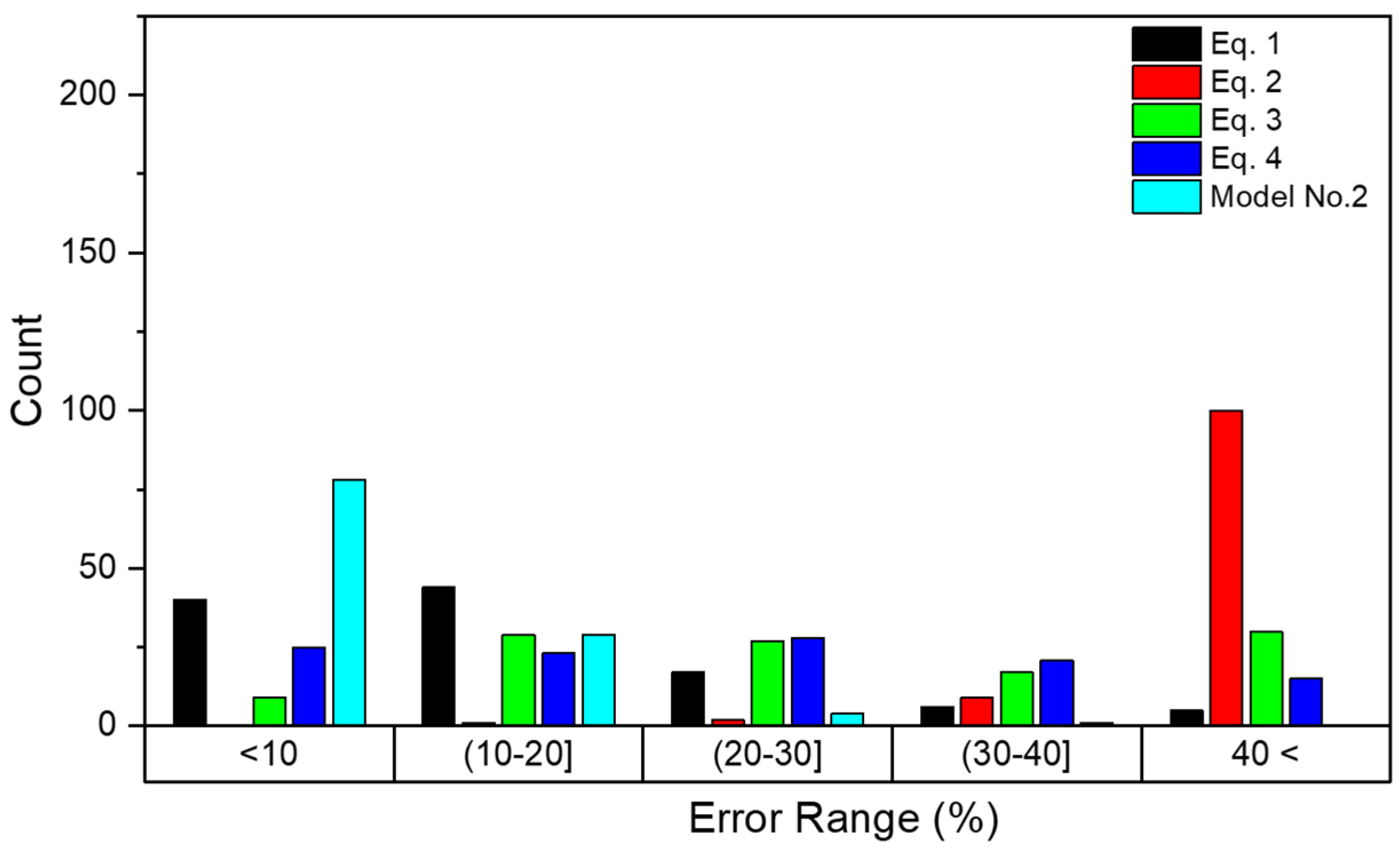
	Model No. 2	206	122	58	14	2	0.06	46.57

provides detailed information about the error distribution of each model across various ranges, while Figure 14 and Figure 15 depict the error distribution. Figure 14 is based on the cylindrical dataset, while Figure 15 is based on the cubic dataset. According to Table 8 and Figure 14, it is clear that Model No. 2 exhibits superior performance, with a significantly higher count of errors within the 10% range and minimal counts in other categories. Additionally, the minimum error of 0.1% and maximum error of 33.6% in CS prediction for cylindrical data confirm this. In contrast, Equation (2) shows a concerningly high number of errors exceeding 40%.

For the cubic dataset, as shown in Table 8 and Figure 15, Model No. 2 exhibits the best performance in the below 10 percent error (<10%) range with 206 predictions but also has a moderate maximum error of 46.6%. Overall, Model No. 2 demonstrates the most robust performance for lower error ranges, while Equation (6) shows the lowest maximum error among all models.

Table 9. The average value of MAPE based on the range of CS for cylindrical data.

CS Range (MPa)	Average MAPE (%)
	Equation (1)	Equation (2)	Equation (3)	Equation (4)	Model No. 2
(0–20]	23.70	71.38	50.95	16.99	8.96
(20–35]	11.01	61.76	29.08	13.81	8.61
(35–50]	14.72	62.61	16.32	31.72	4.66
(50–65]	11.60	49.04	21.00	33.12	6.95
65<	1.95	34.99	26.67	30.70	12.57

and

Table 10. The average value of MAPE based on the range of CS for cubic data.

CS Range (MPa)	Average MAPE (%)
	Equation (5)	Equation (6)	Equation (7)	Equation (8)	Model No. 2
(0–20]	29.53	18.74	67.41	83.11	19.93
(20–35]	23.33	10.10	39.17	36.41	10.10
(35–50]	20.66	17.95	19.64	6.83	9.48
(50–65]	18.89	27.40	10.00	13.41	8.96
65<	7.11	39.15	9.39	28.71	15.36

show the average MAPE for different models across various ranges of CS measured in MPa. Table 9, which is based on the cylindrical dataset, reveals that Model No. 2 exhibits the lowest MAPE across most CS ranges, making it the most accurate and reliable model overall. Specifically, it achieves the best performance in the ranges (0–20 MPa), (20–35 MPa), (35–50 MPa), and (50–65 MPa), indicating its robustness across a wide spectrum of CS values. In the highest CS range (65< MPa), Equation (1) outperforms the others, achieving the lowest MAPE, while Model No. 2’s performance, though still reasonable, is not the best in this range.

According to Table 10, which is based on the cubic dataset, for the lowest CS range (0–20 MPa), Model No. 2 shows the best performance with a MAPE of 19.93%, significantly lower than the other equations. As the CS increases to the 20–35 MPa range, Model No. 2 maintains its leading position with a MAPE of 10.10%, matching the lowest error of the other models. In the 35–50 MPa range, Model No. 2 again performs best with a MAPE of 9.48%, highlighting its consistent accuracy across different CS levels. For the 50–65 MPa range, Model No. 2 continues to show superior performance with an average MAPE of 8.96%, while the other equations vary more in their accuracy. However, for CS greater than 65 MPa, Model No. 2’s MAPE rises to 15.36%, which is still relatively low but not the best in this range, where Equation (5) shows the lowest error of 7.11%.

Figure 16 provides the prediction intervals (PIs) defined in Equation (15) for a 95% probability for various models predicting concrete strength based on the dataset type. The PI indicates the range within which future observations are expected to fall and is computed as follows:

$$Prediction Interval=[\mu -z\sigma ,\mu +z\sigma ]$$

(15)

where $\mu$ represents the mean of the experimental-to-predicted ratio, $\sigma$ is the standard deviation of the experimental-to-predicted ratio, and the z-value corresponding to the selected probability level (z = 1.96 for 95% probability). Accordingly, in Figure 16A, which corresponds to the cylindrical dataset, the ML model demonstrates the narrowest PI, ranging from 0.815 to 1.201, indicating higher consistency and reduced variability in predictions compared to the equations. Equation (3) exhibits the widest PI, spanning from −0.423 to 3.606, reflecting substantial uncertainty and reduced reliability for this dataset type and rendering it ineffective for practical use. Similarly, in Figure 16B, the ML model again outperforms the equations with the narrowest PI (0.709 to 1.290), while equations (e.g., Equations (6) and (8)) show relatively wider intervals, suggesting higher prediction uncertainty. Overall, the ML model consistently shows narrower PIs in both dataset types, implying better reliability and precision in predictions compared to the equations.

5. Prediction Uncertainty

The information provided in the previous section gives a comprehensive overview of the performance of the ML and regression models. However, it is important to note that this comparison may not be entirely fair because the ML model was trained on a large portion of the data (training data), which were also part of the overall dataset used for evaluation in the previous section. A more equitable comparison would involve assessing the performance of each model using only testing data from different sources not seen during the training phase.

Table 11. Comparing the performance of Equations (1)–(4) and Model No. 2 based on testing data of cylindrical geometry.

Parameter	Equation (1)	Equation (2)	Equation (3)	Equation (4)	Model No. 2
MAPE (%)	12.73	53.52	20.35	29.60	9.63
RMSE (MPa)	6.87	25.71	12.41	15.93	5.90
R	0.880	0.881	0.828	0.877	0.897

compares the performance of Equations (1)–(4) and Model No. 2 model across three metrics, MAPE, RMSE, and R, based only on testing data for cylindrical geometry. The proposed ML model shows superior performance in all metrics, with a MAPE of 9.63%, RMSE of 5.90 MPa, and R of 0.897. Overall, the model demonstrates the best performance in terms of error metrics and correlation, indicating its effectiveness.

Table 12. Comparing the performance of Equations (5)–(8) and Model No. 2 based on testing data of cubic geometry.

Parameter	Equation (5)	Equation (6)	Equation (7)	Equation (8)	Model No. 2
MAPE (%)	15.85	14.89	23.26	16.46	14.62
RMSE (MPa)	8.53	11.62	11.03	10.80	7.32
R	0.894	0.946	0.887	0.870	0.880

compares the performance of Equations (5)–(8) and Model No. 2 based on testing data for cubic geometry. The ML model shows superior performance across most metrics, with MAPE of 14.62% and RMSE of 7.32 MPa. Although the ML model’s R value is 0.880, a good result, it is lower than some of the other equations.

For both all data and the testing data, the ML model demonstrates superiority over conventional regression approach for predicting CS in both cubic and cylindrical standard. Previous studies indicate that there is inherent uncertainty in predicting concrete CS [3,10,11]. Moreover, if multiple cores are taken from a similar location within a structure, the results of compressive strength tests will also vary.

Table 11 and Table 12 clearly demonstrate that the ML model exhibits superior reliability and accuracy in predicting new, unseen data (testing datasets). This highlights the model’s robustness in handling unfamiliar inputs. In terms of uncertainty, Figure 16 presents a detailed analysis of the prediction intervals (PIs) for the ML model. The results show that 18 out of 20 testing data points were within the 95% PI for the cylindrical dataset, while all eight testing points from the cubic dataset were within the 95% PI. Hence, the combined prediction accuracy for the testing dataset is 93%, which validates the use of PIs to establish non-deterministic predictions for any required probability level specified by a structure owner and provides further confirmation of the model’s effectiveness and consistency in making accurate predictions across different data types.

6. Discussion and Roadmap

According to Figure 7D, which relates to core data, it was noted that the dataset with ID No. 17, used as testing data in the modeling process, follows a different pattern compared to the other core data used for training. This discrepancy affected the model’s performance for the core data, as shown in Table 9. It is possible to filter outlier data to potentially improve model performance; however, this type of filtering was avoided in this study to highlight a major challenge regarding the collection of data from the field. By investigating the sources of the datasets listed in Table 2, it can be seen that different procedures were utilized to extract the data in each case. Moreover, the size of the core samples differs: Dataset No. 11 did not provide the size of the cores [22]; Dataset No. 12 contains core data with a diameter of 84 mm, while the length of the samples was not provided [13]; Dataset No. 13 includes core data with a size of 100 mm × 200 mm [11]; and Dataset No. 17 consists of core data with a size of 105 mm × 105 mm [63]. The low height-to-diameter ratio of the latter group may have contributed to the observed discrepancies (i.e., higher compressive strength than expected). Needless to say, these differences will affect the quality of the data, as well as the performance of the ML model. Given this fact, and in line with the primary objective of such studies—to develop a precise and reliable ML-based method to reduce, and potentially eliminate, the need for core tests in the future—it is important to note that one factor influencing data quality is the methodology used for UPV and RN tests, where human factors can significantly affect the test results.

To improve data quality and enhance the capabilities of future ML models for field applications, it is recommended to implement consistent experimental testing procedures similar to that outlined in Figure 17 and to populate a shared open-access database. This approach aims to improve data quality, model accuracy, and the overall reliability of future models. As shown in Figure 17A, the proposed approach involves the construction of RC slabs with dimensions of at least one meter by one meter and a minimum thickness of 200 mm, based on various mix designs. These slabs could be subjected to different environmental conditions to account for varying boundary conditions in the data. Each slab can be divided into four zones, with testing scheduled at different ages: Zone 1 at 14 days, Zone 2 at 28 days, Zone 3 at 90 days, and Zone 4 at 180 days after casting. The proposed testing procedure involves conducting sequential NDT and DT, including three types of UPV tests (direct, indirect, and semi-indirect, Figure 17B), RN tests conducted both horizontally and vertically (Figure 17C), followed by the extraction and testing of three cores with dimensions of 100 by 200 mm (Figure 17D). This procedure can be repeated for slabs with different specifications to create a comprehensive databank for future ML model development with up to five input parameters. (It should be noted that for many structural members, it may not be possible to obtain direct UPV measurements; collecting multiple measurements for the database enables the development of models for different scenarios.) Given that the concrete strength data in the database is derived from cores with dimensions of 100 by 200 mm—a standard size—the model output will be based on the strength of standard cylindrical cores, in compliance with all relevant codes.

Also, it should be mentioned that ethical considerations related to open-access data must be taken into account in the future. Consent for usage and data protection laws are essential steps in the collection process when developing any ML model.

7. Conclusions

In this study, the uncertainty and prediction intervals of a new machine learning approach for the combined non-destructive testing method of SONREB in predicting concrete strength was thoroughly evaluated. For this purpose, a new machine learning-based model was developed for the first time, capable of distinguishing between cylindrical, cubic, and core specimens. This model was developed on a comprehensive database consisting of 620 collected data points. After the model was developed, its results and reliability were compared with four well-known equations based on cylindrical standards and four well-known equations based on cubic standards. The comprehensive performance analysis in this study was conducted by directly applying the selected equations and the developed model to evaluate concrete strength, without the calibration process in using the SONREB method.

The findings of this study clearly demonstrate that the machine learning-based model is significantly more reliable and accurate than other equations in predicting concrete strength without the calibration process. It is important to note that the results of the presented machine learning model are entirely dependent on the data and the algorithms used. Therefore, it is evident that with advancements in computer processing power, improvements in algorithms, and increased data availability, we can expect to see more accurate and practical models based on artificial intelligence and machine learning in the future. This study effectively shows that the machine learning-based model can outperform traditional mathematical models. Finally, based on the results of the current study, a test procedure and ML model architecture is suggested for future study.

It should acknowledge the limitations of this study, as the proposed model only worked based on the specific range of data it was trained on. Additionally, these data were collected from normal-strength concrete without fibers, specific concrete additives, special concrete mix designs, or concrete with a specific cement type. The data were also based on undamaged concrete under normal conditions (not in specific environmental conditions such as high or low temperatures, or dry or humid conditions), and the data used were based on tests on undamaged concrete specimens. Therefore, it would be beneficial to conduct future studies on each of these limiting factors and their effects on ML model results. It is hopeful that by overcoming these challenges and addressing the mentioned limitations, an efficient AI/ML model can be developed based on the high-quality data in the future. This model, utilizing the low-cost and fast method of SONREB, would enable a more reliable estimation of concrete strength with reduced core testing, ultimately leading to improved safety of the RC structures.