Experimental Study on the Seismic Performance of Confined High Walls of Autoclaved Aerated Concrete Panels Used in Subway Stations

Abstract

This study addresses the unique challenge of the partition walls in subway stations, featuring high height, fire prevention, and located outside the main frames, by introducing a confined autoclaved aerated concrete (AAC) panel wall system. Different from studies on a main frame with infill walls, this study aimed to explore the seismic performance of partition walls, which were fabricated with confined high AAC panel walls and located outside the main frames. A custom-designed partition wall, measuring 6600 mm in height, 3400 mm in width, and 200 mm in thickness, underwent cyclic testing. A detailed analysis of specimen’s failure modes was conducted, focusing on seismic behavior such as hysteresis curves, envelope curves, ductility, stiffness degradation, and energy-dissipation capacity. Additionally, the study delved into shear deformation, relative slippage between AAC panels, and reinforcement strains within the specimen. Finally, the D-value method for calculating the initial stiffness of the confined high AAC panel walls and the weak sub-structural approach for determining the load-bearing capacity of confined high AAC panel walls were proposed and validated. The results indicate that the strength degradation factor of the confined high AAC panel walls ranges from 0.971 to 0.716. The drift of its upper portion accounts for 76.94–83.63% of the total drift, while the energy dissipation factor of its upper portion is 0.8–4.8% higher than that of the entire specimen. The yield and ultimate drift rotations of the entire confined high AAC panel wall and its upper portions satisfy the elastic and elastic-plastic inter-story drift rotation limits specified in the Chinese code. The calculated initial stiffness of the confining frame, obtained using the D-value method, closely aligns with experimental results, with a deviation of only 2.48%. Additionally, the load-bearing capacity calculated using the weak sub-structural approach deviates from the experimental average by just 4.30%.

1. Introduction

Subway stations have spacious interiors, with spans ranging from 8 m to 15 m and heights from 6 m to 8.4 m. To divide the internal space into separate rooms, partition walls are commonly utilized. Given their larger dimensions, interior partition walls of subway stations are typically constructed using masonry reinforced with non-structural beams and columns. Nevertheless, traditional masonry walls come with several drawbacks. These include unfavorable working conditions, time-consuming construction processes, the need for extensive work areas, considerable environmental pollution, and challenges in transporting construction materials and waste within the limited indoor space. Consequently, these factors contribute to increased labor demands and higher construction expenses.

The construction industry has witnessed rapid advancements in prefabricated wall systems, leading to the widespread adoption of AAC blocks and panels in buildings. In recent years, the railway transportation sector in China has also embraced prefabricated wall systems. For instance, in 2016, the Yuanjiadian subway station on Changchun Metro Line 2 became the first subway station to be constructed using prefabricated wall systems. Similarly, in 2017, the equipment rooms of Wuxianghu station on Nanning Metro Line 3 were built using prefabricated potassium-sodium-stone lightweight wall systems. Additionally, in 2018, AAC panels were utilized for constructing interior partition walls in subway stations on Beijing Metro Line 19 [1].

AAC blocks or panels are lightweight and possess good thermal insulation properties, excellent fire resistance, energy efficiency, and environmental friendliness. They find extensive use in prefabricated floor and wall systems [2,3]. The advantages of AAC blocks include their small size, facilitating transportation and installation. However, they exhibit low load-bearing capacity and poor crack resistance. Commonly employed methods to enhance the entire strength and load-bearing capacity of AAC block structures include the following [4,5]: (a) Configuring non-structural columns and beams, and embedding reinforcement bars in bed joints to create a combination of reinforcement bars, blocks, non-structural columns, and non-structural beams [6]; (b) installing flat trusses reinforcement in the bed joints of AAC block structures [7]; and (c) applying high-ductility fiber-reinforced concrete on both sides of AAC block walls or plastering the outer and middle parts of AAC block walls at appropriate intervals to form high-ductility concrete strips [8,9].

In multi-story or high-rise buildings where AAC blocks are used as partition walls or exterior walls, it is necessary to install non-structural columns. Reinforcement bars should be embedded in the bed joints at intervals of 500–800 mm in the vertical direction to ensure entire integrity. In frame structure design, the load-bearing capacity and lateral resistance of infill walls are often overlooked. The diagonal strut effect of infill walls improves the lateral resistance of the frame, posing challenges in accurately calculating static and dynamic performance, resulting in significant design errors. Therefore, considerable attention has been given to the interaction between infill and frame, as well as the calculation of the diagonal strut effect of infill walls [10,11].

To improve design accuracy, it is necessary to reduce the diagonal strut effect of infill walls during construction while ensuring the entire integrity and safety of the walls [12]. For infill walls of the frame structure, a 20 mm gap can be left on both sides and the top of the wall, with U-shaped connectors installed between the wall and the frame to reduce the diagonal strut effect and ensure out-of-plane stability.

AAC panels can serve as internal or external walls in framed structures. When used as internal walls, U-shaped, L-shaped, or corner connectors should be installed at the top and bottom of the panels. Additionally, a 20 mm gap should be left on both sides and the top of the panel assemblies, with thermal-insulation flexible matrix used to fill the gap. This construction method ensures both out-of-plane stability and reduces the diagonal strut effect of AAC panel walls [13,14,15,16].

For steel frame structures, AAC panels can be used as infill walls or connected to the steel frame along the outer side of frames. The connection between the steel frame and the external AAC panels can be achieved through the following methods [17,18,19,20]: (a) Using hooked bolts or Z-shaped rocking connectors to connect each AAC panel to the steel frame beams from the outer side of the frames. (b) Connecting AAC panels into an assembly using connectors or confining frames. Fixed supports should be installed at the bottom of the assemblies, and sliding supports should be installed at the top. Research shows that in steel frame external wall systems, the diagonal strut effect of the wall panels is small and has minimal impact on the lateral stiffness and resistance of the steel frame.

The aforementioned research provided comprehensive insights into the construction methods, load-bearing capacities (both in-plane and out-of-plane) of infill walls, the calculation of the diagonal strut effect in these walls, and methods for reducing this effect in AAC block and panel structures with floor heights of approximately 3 m. However, there was still a lack of research regarding the construction methods and seismic performance of high AAC panel partitions, particularly in large buildings with heights ranging from 6 to 8.4 m, located outside the main structural frame.

When AAC panels are directly used as partition walls in subway stations to divide spaces, each panel must reach lengths of 6–8.4 m. To meet lifting requirements, the thickness of these panels typically exceeds 300 mm, resulting in significant material waste. Furthermore, AAC panels of such length and weight present significant issues in terms of outdoor transportation and indoor installation, and challenges that current technology cannot easily resolve.

To address these challenges—particularly for partition walls in subway stations that require large height, fire resistance, seismic stability, and cost efficiency—a new configuration method, known as the ‘confined AAC panel wall system’, has been introduced. This system employs AAC panels of more manageable lengths (approximately 3–4 m) and weights (less than 300 kg), making them easier to transport and install. These panels are readily available on the Chinese market at a low cost. The confined AAC panel wall system was successfully implemented in six subway stations along Qingdao Metro Line 6 in 2022. In practical applications, when the height of the confined AAC panel wall system is relatively low (less than 4 m), it can be used in residential or commercial buildings.

The confined AAC panels wall system offers several advantages: (a) All components are prefabricated, featuring moderate dimensions and weights for easy transportation and installation. (b) The need for temporary support components is minimized, requiring only a small amount during the confining frame installation. (c) Firm connections are ensured through cast-in-place joints, L-shaped connectors, and mortise and tenon, guaranteeing robust safety and stability of the wall system. (d) Steel connectors are embedded in the concrete, eliminating the need for special fire protection measures and subsequently reducing construction costs. Given these advantageous features, the confined AAC panel wall system proves highly suitable for widespread application in spacious indoor spaces.

This study is divided into five sections. Section 1 introduces the research progress of AAC panel structures, the application of AAC walls in subway stations, and the challenges they face, proposing a fully prefabricated confined AAC panel wall system. Section 2 and Section 3 describe the structural configuration and connection methods of the confined AAC panel wall system, including the design of specimens, the physical and mechanical properties of materials, experimental setup and instrumentation, and the loading procedure. Section 4 presents the experimental results and analysis, detailing the observed phenomena, and analyzing the failure modes of the specimens and the different aspects of seismic performance. It also includes an analysis of the shear angle and relative slippage of the AAC panels, elaborations on the process of calculating the initial stiffness of confined high AAC panel walls using the D-value method, and an overview of the sub-structure method for calculating the load-bearing capacity of high-confined AAC panel walls. Section 5 summarizes the entire study and presents the conclusions. The research framework is shown in Figure 1.

This research conducted cyclic experiments on a full-scale high AAC panel partition wall confined by columns and beams, analyzed its seismic performance, proposed a stiffness degradation model and a shear angle model, developed a method for predicting its initial stiffness, and introduced a weak sub-structural approach for determining its lateral load-bearing capacity.

The results indicate that, from an engineering perspective, the influence of the door frame position on the confined high AAC panel wall can be disregarded. Due to the strengthening effect of the door frame in the lower portion of the specimen, failure predominantly occurred in the upper portion, with shear failure observed at the confining frame joints and the corners of the AAC panels. The AAC panels and the confining frame exhibited effective cooperative deformation, dissipating seismic energy through relative slippage. After the failure of the confining frame, the lateral load-bearing capacity of the wall primarily relied on the AAC panels. Moreover, the infill AAC panels significantly contributed to the ductility and deformation capacity of the confined high AAC panel wall system. The top beam of the confined high AAC panel wall experienced upward bending due to the diagonal strut effect of the AAC panels, resulting in vertical flexural cracks on its upper portion. Additionally, the slippage between the side panels was less pronounced compared to that between the middle panels, indicating a gradual reduction in the confining effect of the top beam on the panels from the sides toward the center.

2. Design of Specimen

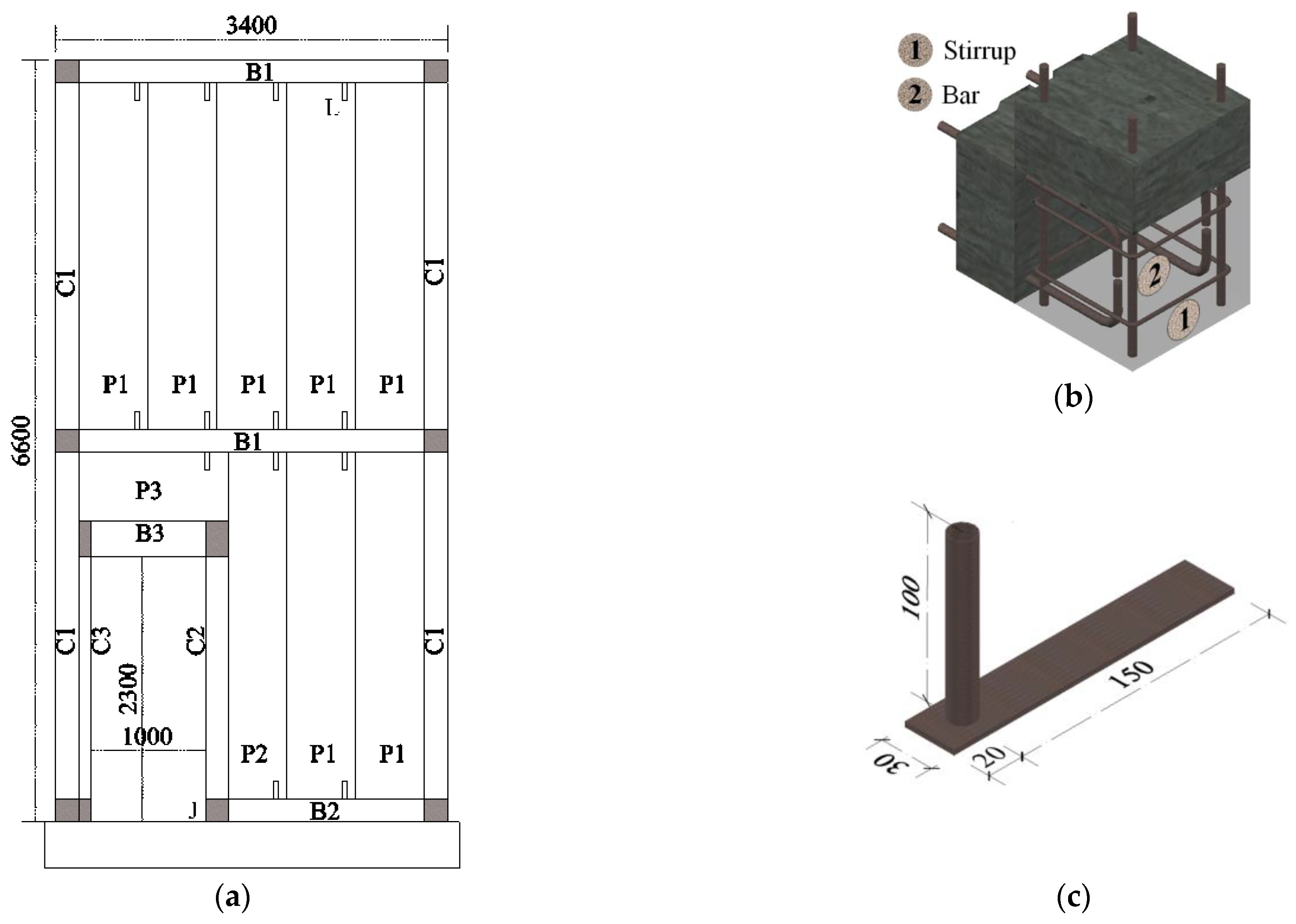
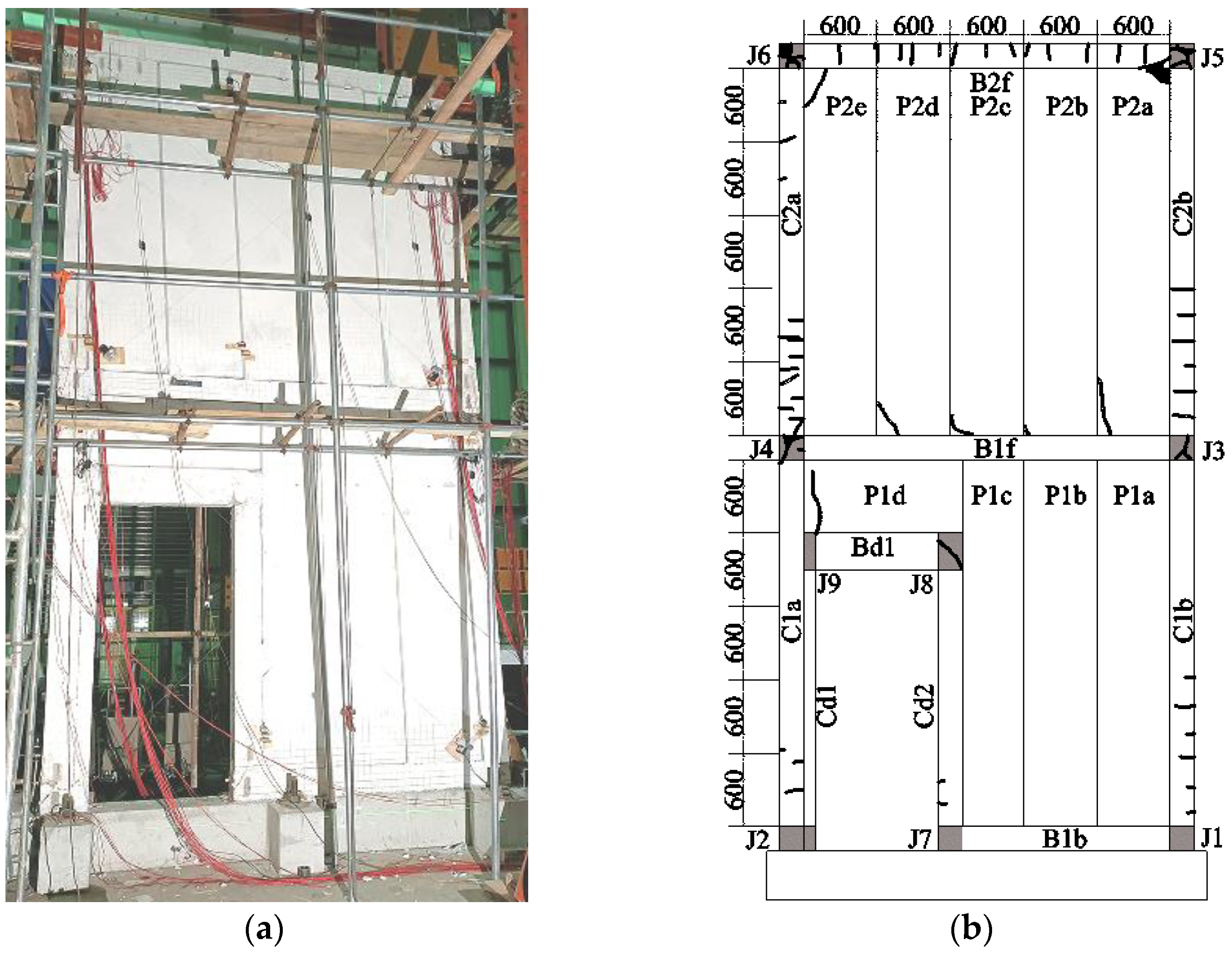
Partition walls in subway stations confined with confining columns and beams consist of confining beams and columns, AAC panels, and cast-in-place joints. The specimen, with a width of 3400 mm and a height of 6600 mm, is shown in Figure 2a, representing the confined AAC panel wall system with a door frame in the lower portion. The specimen consisted of four precast columns ‘C1’, two precast beams ‘B1’, and one precast beam ‘B2’. The clear width of the door opening was 1000 mm, with a clear height of 2300 mm. The door frame was composed of two precast columns ‘C2’ and ‘C3’, along with one precast beam ‘B3’. In Figure 2a, the specimen includes seven AAC panels represented by ‘P1’, one AAC panel of ‘P2’ and one of ‘P3’. The AAC panels of ‘P2’ and ‘P3’ were obtained by cutting the standard panel ‘P1’. The sizes of the precast components are detailed in

Table 1. Sizes of members.

Symbol	Width (mm)	Depth (mm)	Length (mm)
P1	600	200	3000
P2	500	200	3000
P3	600	200	1300
B1	200	200	3000
B2	200	200	1700
B3	200	300	1300
C1	200	200	3000
C2	200	200	2100
C3	100	200	2100

.

During the installation process, the initial step involved positioning and temporarily securing the precast components of the confining frame and the door frame. Subsequently, the cast-in-place joints, denoted by the symbol ‘J’ in Figure 2a, were poured. The configuration of these joints is shown in Figure 2b. Longitudinal reinforcements were connected by welding, while stirrups were welded onto the longitudinal reinforcements. After the curing process of the cast joints was completed, the AAC panels were installed in sequence. When placing each AAC panel, L-shaped connectors must be driven into one of both ends of the panel (as shown in Figure 2c). Once a panel was correctly positioned, the exposed part of the steel plate of the L-shaped connector was fixed to the confining beam using explosive nails. These L-shaped connectors were made by welding a steel pipe with a diameter of 15 mm and a thickness of 1.5 mm to a steel plate with a thickness of 3 mm. Additionally, the steel pipe of the L-shaped connector was kept 100 mm away from the edge of the panel.

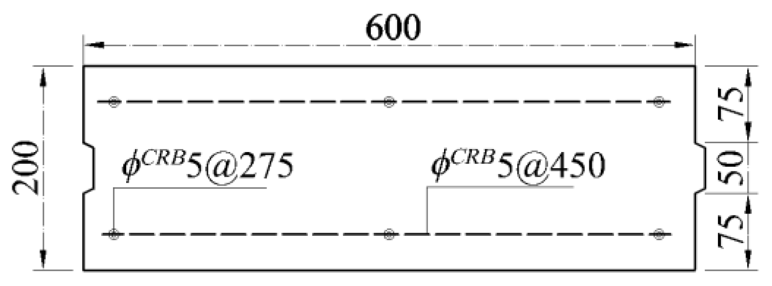
The AAC panels utilized in this system were of the type of UBLOCK-B06-A5.0 (Deyang UBLOCK New Building Materials Co., Ltd., Deyang, China), having a compressive strength of 5.0 N/mm² and a density of 0.8 kN/m³. The details of the AAC panel ‘P1’ are shown in Figure 3, while the configuration and reinforcement of the prefabricated beams and columns are shown in Figure 4. During assembly process, connections are established between the prefabricated beams and columns and the AAC panels using mortise and tenon connections and L-shaped connections.

For AAC panels, cast-in-place joints, and precast components, three cubic specimens were prepared for each, measuring 150 mm × 150 mm × 150 mm. The test results for the cubic compressive strength of the AAC panels, cast-in-place joints, and precast components are shown in

Table 2. Mechanical parameters of concrete.

Components	fcu	fcu,k	fck	ftk	fc	ft	Ec
	(N/mm2)	(N/mm2)	(N/mm2)	(N/mm2)	(N/mm2)	(N/mm2)	(N/mm2)
AAC panels	5.30	5.17	--	--	--	0.5	2100
Joints	34.63	32.41	21.68	2.06	15.48	1.47	30,576
Precast components	33.00	32.41	21.68	2.10	15.48	1.50	30,576

. In accordance with the Chinese Code for Design of Concrete Structures (GB50010-2010) [21], the standard compressive strength f_cu,k for the concrete cubes with the sizes of 150 mm × 150 mm × 150 mm, the standard compressive strength for concrete prisms f_ck, the standard tensile strength f_tk, the design compressive strength for concrete prisms f_c, the design tensile strength f_t, and the elastic modulus of concrete were calculated. These are all given in Table 2.

The steel bars were made by Kunming Steel Holding Co., Ltd., Kunming, China. The longitudinal reinforcements for the precast components were ribbed steel bars with a 12 mm diameter and a grade of HRB400. The stirrups were plain steel bars with a diameter of 6 mm and a grade of HPB300. For the AAC panels, cold-rolled ribbed steel bars with a 5 mm diameter and a grade of CRB 550 were used. Three samples of each type of reinforcement underwent testing, and the yield strength f_y, the maximum tensile strength f_u, and elastic modulus E of the reinforcement are detailed in

Table 3. Mechanical parameters for steel bar.

Grade	Diameter	fy	fu	E
	(mm)	(N/mm2)	(N/mm2)	(103 × N/mm2)
HPB300	6	410	511	193
HRB400	12	407	592	205
CRB550	5	500	550	200

.

3. Experimental Program

3.1. Setup and Instruments

As shown in Figure 5, the base of the specimen was anchored to the reaction floor using ground anchor bolts, and the longitudinal reinforcements at the bottom of the specimen were welded to steel plates embedded in the foundation. The actuator was fixed at a height of 6.5 m at the top of the specimen, with a stroke of ±400 mm. Lateral support beams were placed in front and behind the top of the specimen to prevent its out-of-plane movement during the experiment.

Horizontal drifts of the specimen were measured using displacement gauges placed at the heights of −0.2 m at the foundation, 3.3 m at the middle, and 6.5 m at the top of the specimen, designated as ‘D1’, ‘D2’, and ‘D3’, respectively. Wire displacement gauges were positioned diagonally to measure shear deformations in the lower and upper portions, with ‘S1’ and ‘S2’ placed between heights 0.0–3.3 m and ‘S3’ and ‘S4’ between 3.3–6.5 m. Ten digital displacement transducers denoted as ‘RD’ were arranged between components to measure their relative sliding. Five strain gauges with a length of 50 mm were glued 100 mm from each end of precast members to measure concrete strain. A total of 80 strain gauges for measuring the concrete strain were used. Additionally, two strain gauges with a length of 5 mm were pasted on two longitudinal rebars (one strain gauge on each rebar) at a position 50 mm from each end of the precast members to measure rebar strain. A total of 40 strain gauges for measuring the rebar strain were used.

3.2. Loading Procedure

The rightward drift of the specimen was positive, while the leftward drift was negative, corresponding to the push and pull directions of the actuator, respectively. As shown in Figure 6, drift-controlled loading was employed [22], with an increment of 20 mm for target drifts less than 60 mm and 30 mm for target drifts greater than 60 mm. The cycling continued until the lateral load decreased to 85% of the maximum lateral load, at which point the test was terminated.

4. Results and Analyses

4.1. Phenomenon

The overall deformation of the specimen during the experiment is depicted in Figure 7a, and the crack distribution on the specimen after the test and the symbols denoting elements are shown in Figure 7b. With increasing drift, the occurrence and propagation of cracks are detailed in

Table 4. Details of failure phenomenon.

D a (mm)	Cracks				UP b (mm)	SLR c (με)
	Component	Count	Description	Width (mm)
20	‘B1b’	1	Sliding at the joints of between ‘B1b’ and ‘P1a’, ‘P1b’, ‘P1c’	0.2	--	714
40	‘P1d’	1	left side	0.4	--	1314
	‘J3’	1	Sliding at the joint of ‘J3’ and the ‘C2b’	0.2
	‘C2b’	2	250mm and 450mm from the bottom of ‘C2b’	0.2
	‘B2f’	3	Vertical cracks	0.2
60	‘J3’	1	Sliding at the joint of ‘J3’ and the ‘C2b’	2	18–20	1857
		1	Inclined crack	0.1
	‘J4’	1		0.1
	‘J5’	1		0.1
	‘J6’	1		0.1
	‘C2b’	4	250 mm, 450 mm, 750 mm, and 1000 mm from the bottom of ‘C2b’	0.4
	‘C2a’	6	150 mm, 250 mm, 420 mm, 555 mm, 700 mm, and 850 mm from the bottom of ‘C2a’	0.2
	‘B2f’	8	Vertical cracks	0.2
	‘P2a’	1	Upper right corner	2
	‘P2b’	1	Lower left corner	2
90	‘J3’,	--	Inclined crack and spalling	1–2	23	2286
	‘J4’,	--		2–3
	‘J5’,	--		0.1
	‘J6’,	--		0.1
	‘J8’	1	Inclined crack	0.2
	‘P2a’, ‘P2c’, and ‘P2d’	1	Lower left corner	1
120	‘J1’	1	Sliding at the joint of ‘J1’ and the ‘C1b’	0.2	20–25	2457
	‘J2’	1	Sliding at the joint of ‘J2’ and the ‘C1a’	0.2
	‘J3’, ‘J4’, ‘J5’, and ‘J6’	--	Crack extension and widening	--
	‘P2c’	1	Crack widening	8
	‘P2d’	1		5
	‘P2e’	1	Upper left	3
150	‘Cd2’	2	200 mm and 400 mm from the bottom of ‘Cd2’	0.1	28	2657
	‘C1a’	3	300 mm, 550 mm, and 630 mm from the bottom of ‘C1a’	0.2
	‘Pld’	1	widening	11
	‘J8’	1		1
180	‘J3’ and ‘J4’	--	Extension and spalling	--	30	2971
210	‘J3’, ‘J4’, ‘J5’, and ‘J6’	--	Cracks intersecting	--	--	3143

^a D represents the acronym for drift, ^b UP is the acronym for uplift of panels, indicating the height of uplift when the panel tilts within the plane, with one corner as the rotation center and the other corner lifting. ^c SLR represents the strain of the longitudinal reinforcement.

. In Table 4, the term ‘cracks’ refers to cracks along the directions of the bending moment of each component, and the ‘width’ of cracks indicated the maximum crack width of the cracks. Based on Table 4 and Figure 7b, the following observations can be made:

When the drift was less than 20 mm, the interaction between AAC panels and the confining frame was relatively small. As the drift increased, the panels moved horizontally with the confining frame, and the lateral load was primarily borne by the confining frame. Minor slippage occurred between beam ‘B1b’ and panels ‘P1a’, ‘P1b’, and ‘P1c’.

When the drift ranged from 20 mm to 150 mm, the interaction between the panels and the frame gradually strengthened as the drift increased.

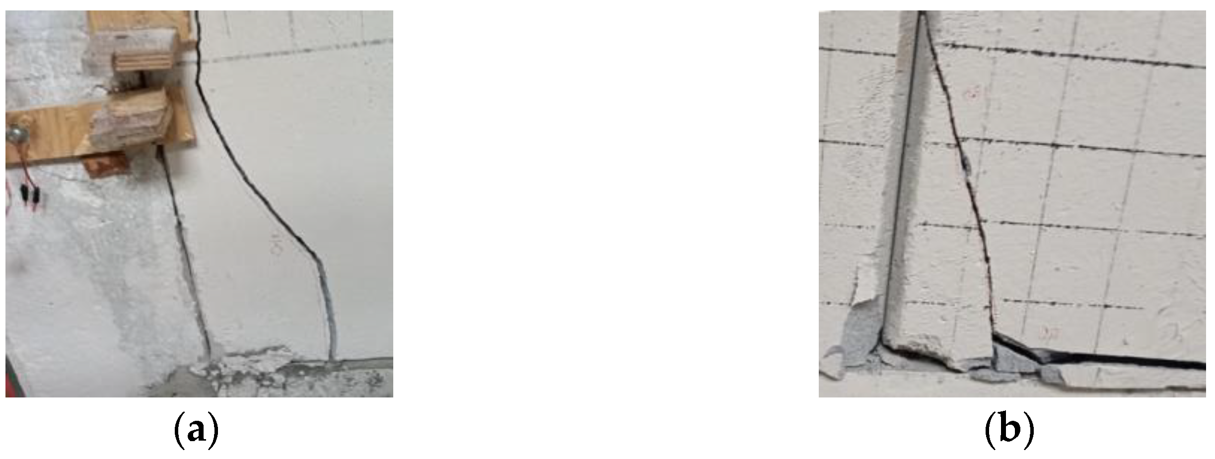
At a drift of 40 mm, cracks appeared on panel ‘P1d’ (see Figure 8a), and small flexural cracks appeared at the lower part of column ‘C2b’ of the upper frame. The top beam ‘B2f’ of the upper frame bent upward, developing vertical cracks.

At a drift of 60 mm, the longitudinal reinforcement in the upper columns approached yielding, with a strain of 1895 με. Multiple flexural cracks were observed in columns ‘C2a’ and ‘C2b’ of the upper frame, while diagonal cracks appeared in the upper frame’s joints ‘J3’, ‘J4’, ‘J5’, and ‘J6’. Diagonal cracks also developed at the lower corners of the upper panels ‘P2a’ and ‘P2b’.

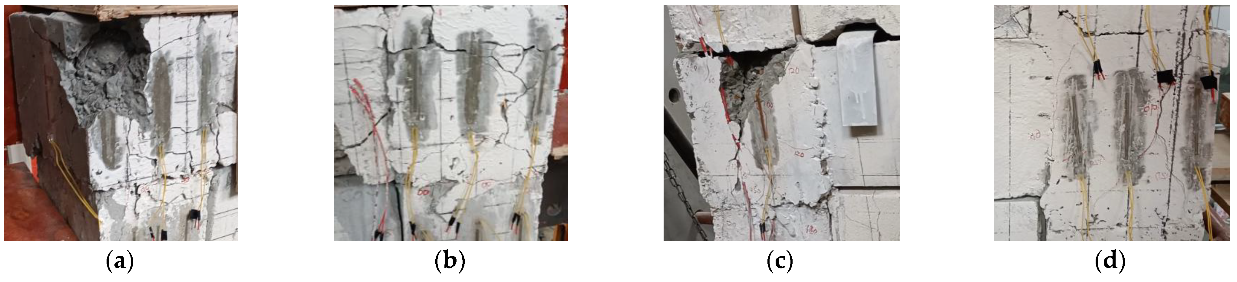
At a drift of 90 mm, the longitudinal reinforcement in the upper columns yielded, with a strain reaching 2286 με. Shear failure occurred at the lower corners of AAC panels ‘P2a’, ‘P2c’, and ‘P2d’ (see Figure 8b and Figure 9b).

At a drift of 120 mm, the diagonal cracks in the upper frame’s joints ‘J3’, ‘J4’, ‘J5’, and ‘J6’ widened progressively. Cracks in the upper AAC panels also widened, with a maximum width of 8 mm.

At a drift of 150 mm, the confined AAC panel wall system reached its maximum lateral load-bearing capacity, and multiple flexural cracks appeared in the lower frame columns. The concrete at the joints of the upper frame began to spall (see Figure 9).

When the drift exceeded 150 mm, ‘joint hinges’ formed at the upper frame’s joints, turning the upper frame into a mechanism unable to continue bearing lateral loads. The lateral loads were then primarily carried by the AAC panels. The diagonal strut effect of the AAC panels contributed to improving the ductility and deformation performance of the confined AAC panel wall system.

From the experiment, it was observed that, due to increased stiffness and lateral resistance from the door frame within the lower portion of the specimen, multiple flexural cracks appeared in the columns and beams of the upper portion. The deformation and failure of the specimen were mainly concentrated in the upper portion.

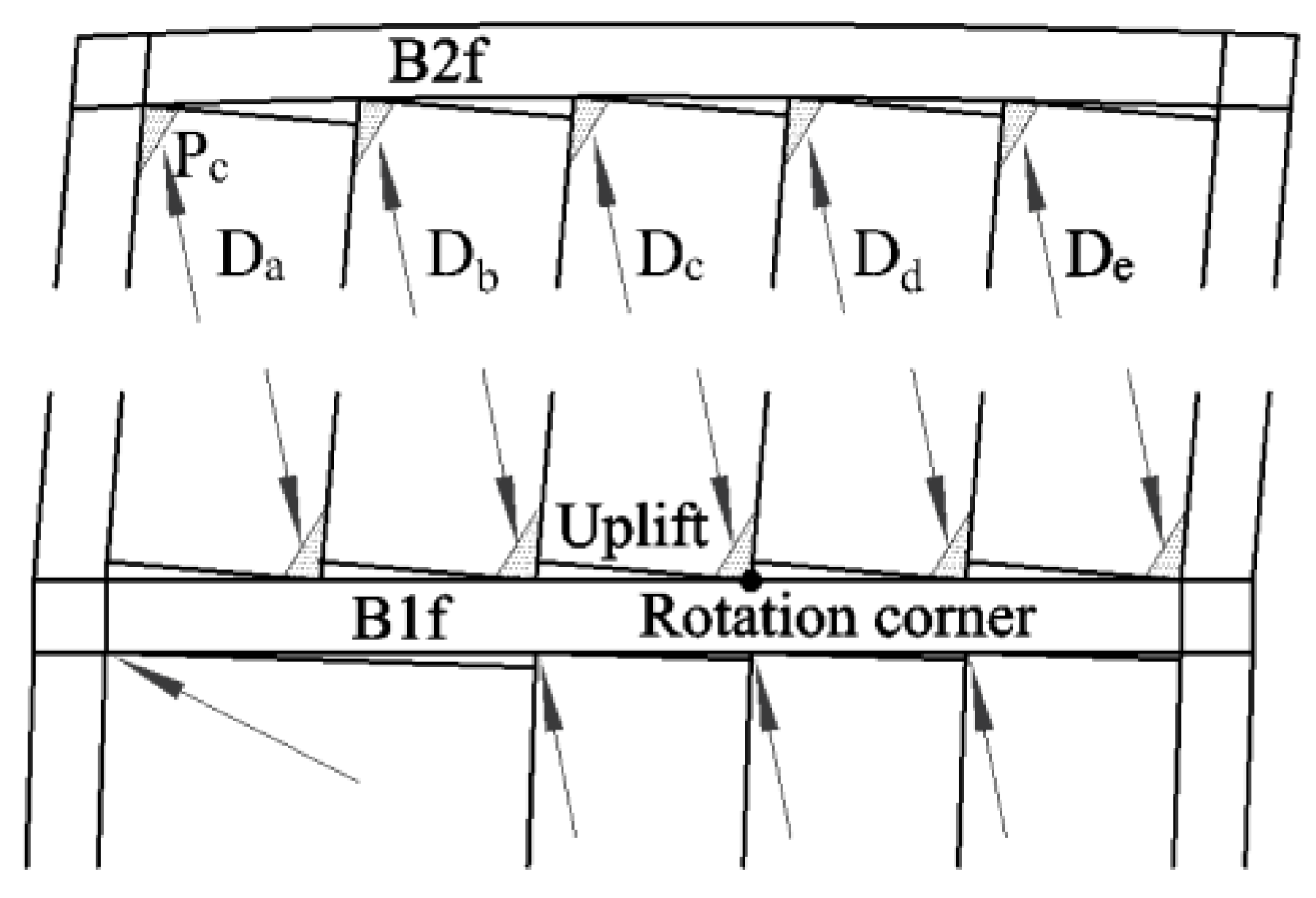
As shown in Figure 10, with the increasing drift of the specimen, each AAC panel rotated around one of its bottom corners, resulting in the other bottom corner of each panel uplifting and making the AAC panels interact with the horizontal components ‘B1f’ and ‘B2f’. As shown in Figure 10, under the diagonal strut effect of upper and lower panels, component ‘B1f’ was balanced in vertical forces and showed no observable flexural cracks. ‘B2f’ experienced upward bending due to the diagonal strut effect from the AAC panels, resulting in vertical flexural cracks on its upper portion.

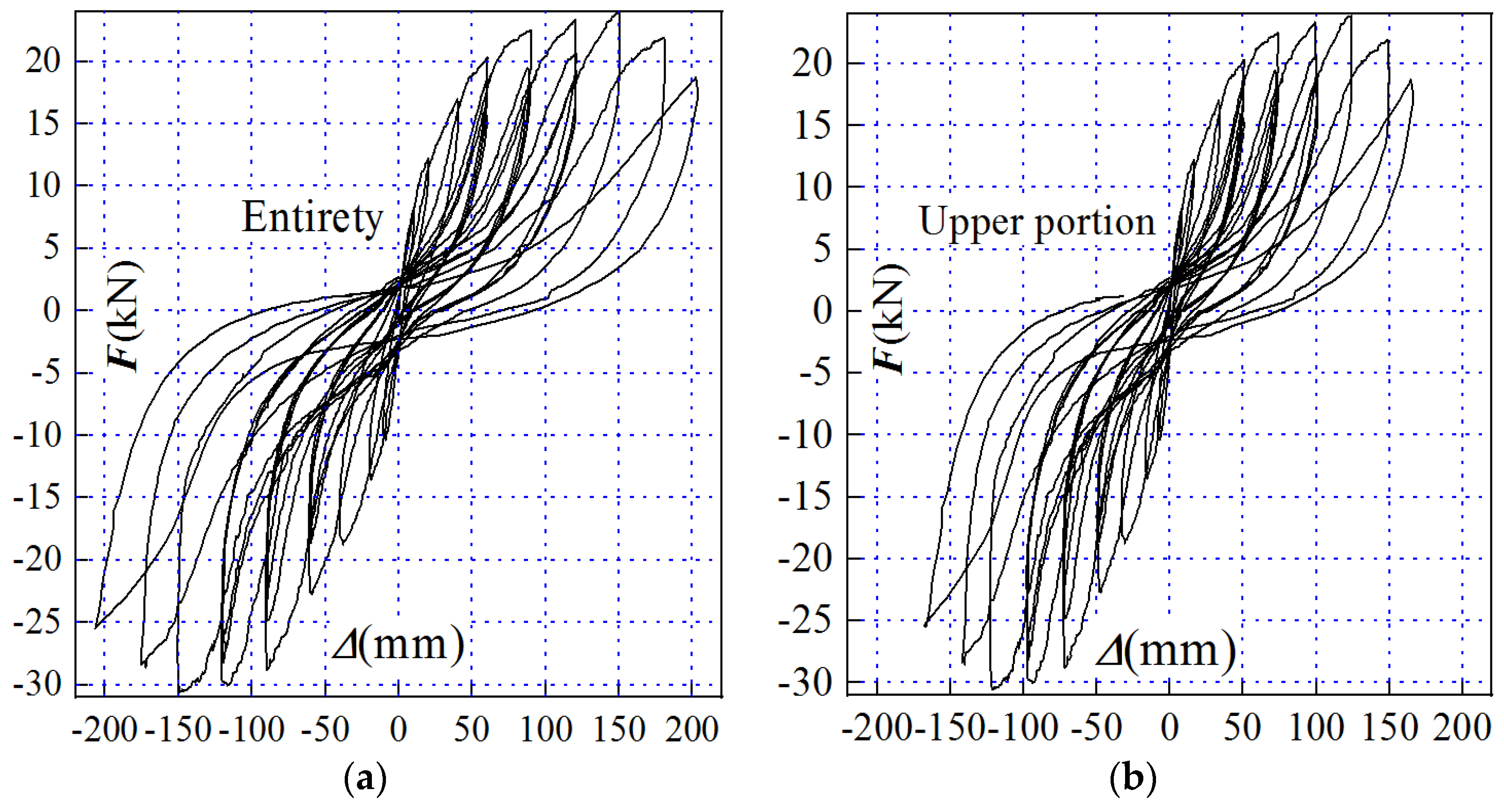
4.2. Hysteresis Curves

The hysteresis curves for the specimen and its upper portion are illustrated in Figure 11. When the drift of the specimen is less than 20 mm, the hysteresis curve showed an outward convexity in both the ascending and descending segments, resembling a ‘spindle’ shape. As the drift ranges from 20 mm to 40 mm, a slight pinching occurs in the middle of the descending segment, forming a ‘bow’ shape. When the drift exceeds 40 mm, the ascending segment of the hysteresis curve becomes concave, presenting an ‘S’ shape.

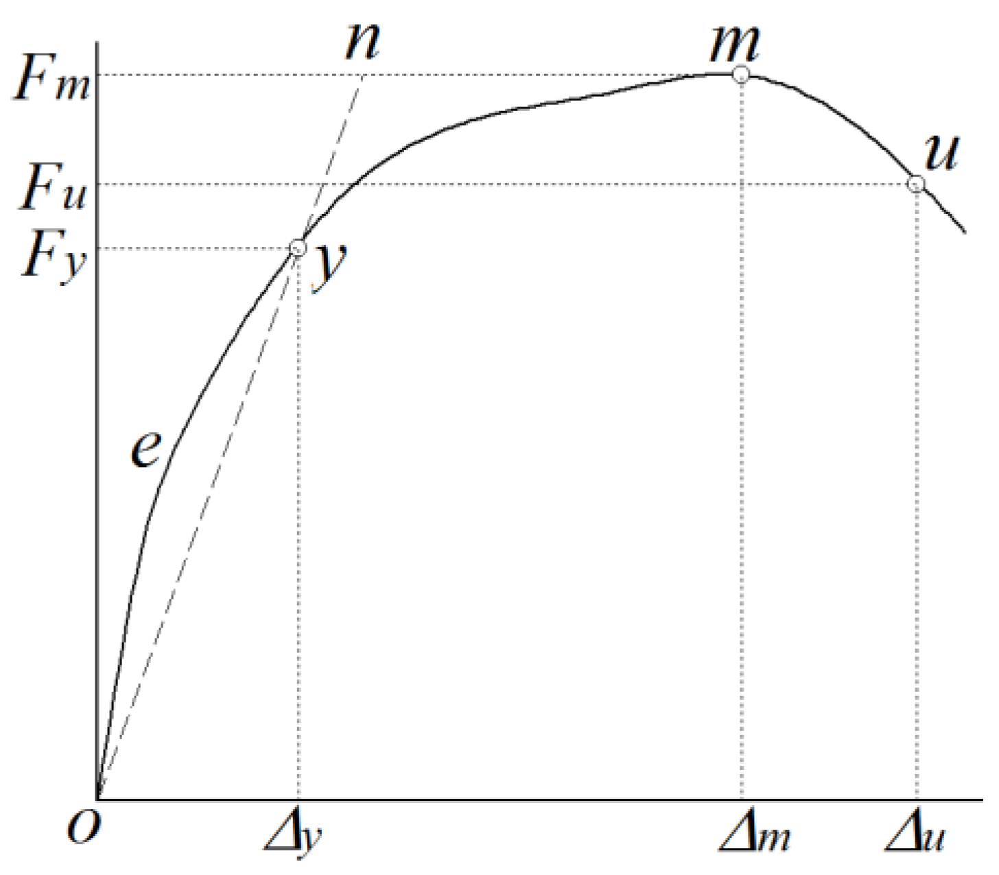
4.3. Envelope Curves

The determination method for key points on the envelope curves is illustrated in Figure 12. The yield point is identified using an energy-based approach. Through mathematical adjustments, the coordinates of the yield point ‘y’ are obtained by positioning the point ‘y’ in Figure 12 to make the areas under the curves ‘o-e-y-o’ and ‘y-n-m-y’ equal. The point ‘m’ is the peak load, while the point on the descending segment of the envelope curve where the force is 0.85 F_m is identified as the ultimate point and denoted by ‘u’. In Figure 12, the symbol ‘F_y’ is the yield load, ‘F_m’ is the peak load, ‘F_u’ is the ultimate load, ‘Δ_y’ is the yield drift, ‘Δ_m’ is the peak drift, and ‘Δ_u’ is the ultimate drift [16].

The entire and upper portion envelope curves of the specimen are presented in Figure 13, with key points for both the specimen and its upper portion detailed in

Table 5. Key points.

Key Points	Symbol	Entire Specimen		Upper Portion
		Push (+)	Pull (−)	Push (+)	Pull (−)
Yield	Δy (mm)	47.024	47.760	38.175	38.306
	Fy (kN)	18.182	20.571	17.980	20.507
	θy (Rad)	1/138	1/136	1/84	1/84
Peak	Δp (mm)	150.225	149.598	124.049	121.759
	Fp (kN)	23.904	30.566	23.904	30.566
	θp (Rad)	1/43	1/43	1/26	1/26
Ultimate	Δu (mm)	191.066	200.888	156.328	162.401
	Fu (kN)	20.318	25.981	20.318	25.981
	θu (Rad)	1/34	1/32	1/20	1/20
DI	β	4.063	4.206	4.095	4.240
ADI	βave	4.135		4.167

. In Table 5, the symbol Δ_y is the yield drift, Δ_p is the peak drift and Δ_u is the ultimate drift. The symbol F_y is the yield load, F_p is the peak load, and is F_u the ultimate load. θ_y is the yield drift rotation of Δ_y/h_f, θ_p is the peak drift rotation of Δ_p/h_f, and θ_u is the ultimate drift rotation of Δ_u/h_f; in which h_f is equal to 6500 mm for entire specimen and is equal to 3200 mm for the upper portion. The symbol ‘DI’ is the acronym of the ductility index, and ‘ADI’ is the acronym of the average ductility index of both the positive and negative ductility index.

From Figure 13 and Table 5, it is observed that the drift of the upper portion constitutes 76.94–83.63% of the entire drift at every intended drift. Considering the potential lack of symmetry in components arrangement during construction, in the push and pull directions, the envelope curves are asymmetrical, with the peak load in the pull direction exceeding that in the push direction by 27.87%, while their peak drifts are similar. The yield, peak, and ultimate drifts are comparable in both push and pull directions, with the yield drifts being 0.31 times the peak drifts in both pull and push directions.

As illustrated in Figure 5, the door frame in the lower portion of the specimen was positioned on the left side, potentially causing differential effects on the drift in the push and pull directions.

Table 6. Entire drift and the drift of the lower portion.

Push (+)		Pull (−)		DIF c
DES a (mm)	R b	DES (mm)	R
10.38	23.06%	−8.93	22.75%	0.31%
20.16	19.43%	−19.00	16.86%	2.57%
39.81	16.80%	−37.99	18.24%	−1.44%
60.21	16.37%	−59.37	20.00%	−3.63%
89.93	18.05%	−89.87	20.06%	−2.00%
120.28	17.60%	−116.75	19.36%	−1.76%
150.23	17.42%	−149.60	18.61%	−1.19%
179.83	17.56%	−172.31	18.68%	−1.12%
202.29	18.70%	−206.75	19.35%	−0.65%

^a DES is the drift of the entire structure (in mm). ^b R is the ratio of the drift of the lower portion to the DES. ^c DIF is the R in push minus the R in pull.

presents data on both the entire drift and the drift of the lower portion. Analysis of the table reveals that when the drift was 20 mm or less, the diagonal strut effect of the panels was relatively weak. Consequently, the drift of the lower portion in the push direction surpassed that in the pull direction by approximately 0.31–2.57%.

As the drift exceeded 20 mm, the diagonal strut effect of the panels gradually intensified. Due to the asymmetry in panel arrangement, the drift of the lower portion in the push direction became less than that in the pull direction, by approximately 0.65–3.63%. With an increasing drift, the difference in the drift of the lower portion between the two directions diminished. From an engineering perspective, the impact of the position of the door frame on the drifts in both push and pull directions is less than 5%. Therefore, this influence can be disregarded in the analysis.

4.4. Ductility Index and Drift Rotation

The magnitude of structural ductility is typically expressed using the ductility index β [16], which is defined as follows:

$$\beta ={\Delta }_u/{\Delta }_y,$$

(1)

in which Δ_u is the ultimate drift, and Δ_y is the yield drift.

As shown in Table 5, the range of the ductility index for the entire specimen is from 4.063 to 4.206. The range of the ductility index for the upper portion of the specimen is from 4.095 to 4.240.

According to the Chinese standard of the Code for Seismic Design of Buildings (GB50011-2010) [23], for concrete frame structures, the value of 1/550 is the elastic inter-story drift rotation limit, the value of 1/50 is the elastic-plastic inter-story drift rotation limit. As shown in Table 5, the range of the yield drift rotation θ_y is from 1/138 to 1/136, surpassing the value of 1/550 for the elastic inter-story drift rotation limit of concrete frame structures. Meanwhile, the range of the ultimate drift rotation θ_u is from 1/34 to 1/32, exceeding the value 1/50 for elastic-plastic inter-story drift rotation limit of concrete frame structures. Moreover, the peak inter-story drift rotation, with a value of 1/43, can also meet the requirements of the Chinese code. From Table 5, it is evident that the yield drift rotation θ_y of the upper portion is 1/84, surpassing the value of 1/550 for the yield elastic local drift rotation limit of concrete frame structures, and the ultimate drift rotation θ_u of the upper portion is 1/20, exceeding the value of 1/50 for the elastic-plastic local drift rotation of limit of concrete frame structures. These results indicate that not only can the entire confined AAC panel walls meet the requirements of Chinese code, but so can its upper portion, suggesting a considerable safety margin.

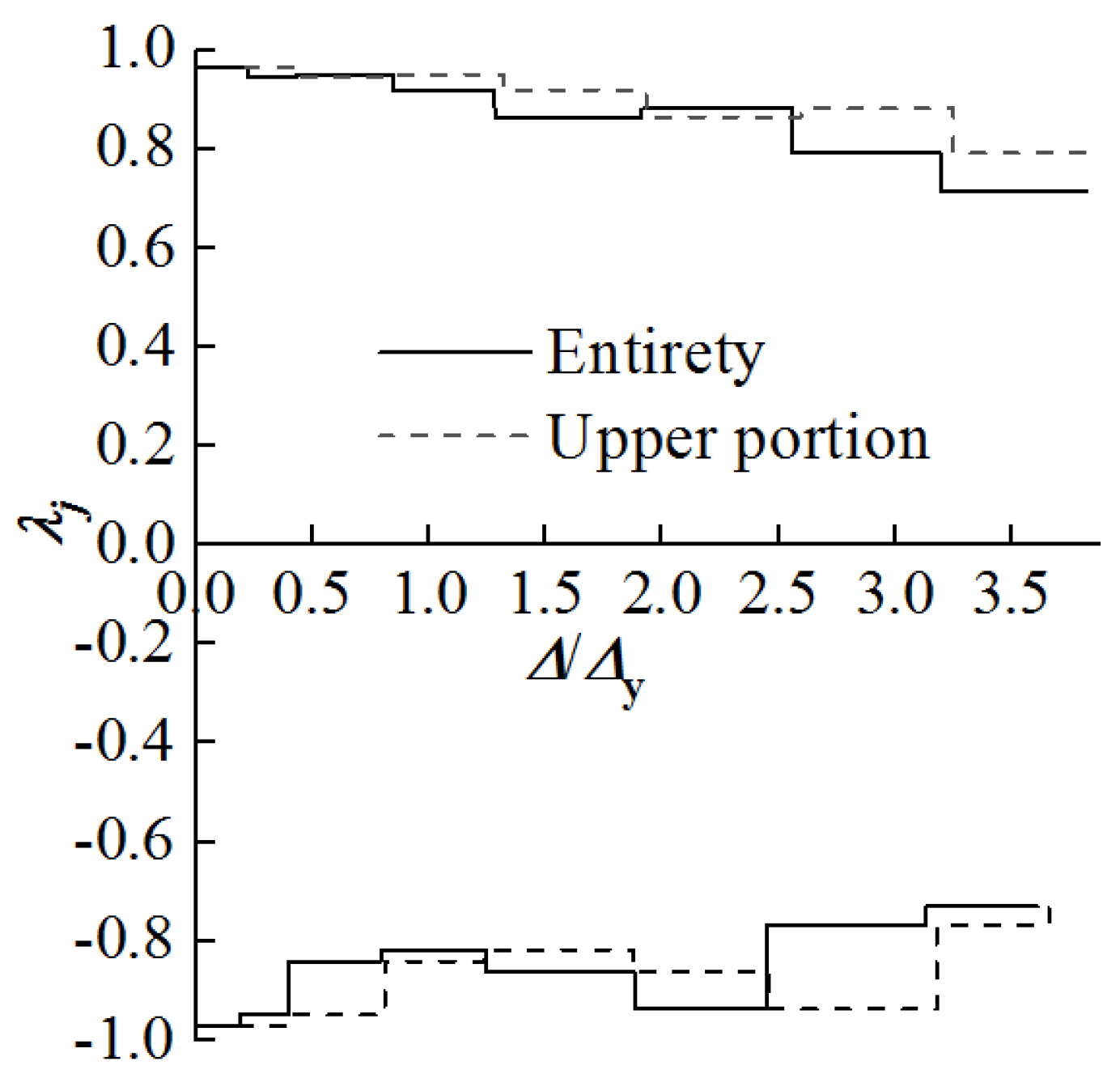
4.5. Strength Degradation

The strength degradation factor can be given as [16]:

$${\lambda }_{ij}=F_j^2/F_j^1,$$

(2)

where λ_ij is the strength degradation factor, F_j¹ is the load at the first cycle and F_j² is the load at the second cycle, and ‘j’ is the intended drift.

The strength degradation factors for the specimen and the upper portion of the specimen are depicted in Figure 14. In Figure 14, the strength degradation factors in the push direction are represented in the first quadrant, while those in the pull direction are represented in the fourth quadrant. The strength degradation factors for both the specimen and the upper portion remain relatively large. The strength degradation factor decreases from 0.971 to 0.716 with the increase of the ductility ratio, indicating that the specimen maintains a robust load-bearing capacity under cyclic loading conditions.

4.6. Stiffness Degradation

The formula for calculating the effective stiffness is given as the following [16]:

$$k_j^i={\displaystyle \sum _{i=1}^n{F}_j^i/}{\displaystyle \sum _j^n{\Delta }_j^i},$$

(3)

in which k_jⁱ is the secant stiffness, F_jⁱ is the lateral load, Δ_jⁱ is the drift, ‘i’ is the number of cycles, and ‘j’ is the intended drift.

Figure 15 illustrates the effective stiffness of both the entire specimen and its upper portion. It is observed that the effective stiffness in the pull direction exceeds that in the push direction for a given ductility ratio, and that the effective stiffness decreases as the ductility ratio increases. Furthermore, as the ductility ratio increases, the effective stiffness of the upper portion of the specimen surpasses that of the entire specimen in both push and pull directions.

Using the experimental data as a benchmark, the model describing the relationship between effective stiffness and ductility ratio for the entire specimen is presented in Equation (4). The fitting parameters ‘a’, ‘b’, and ‘c’ for effective stiffness in both push and pull directions are provided in

Table 7. Parameters of the fitting stiffness degradation curves.

Symbol	a	b	c	R2
Push	0.906	1.685	2.033	0.996
Pull	0.106	2.269	1.651	0.994

. The fitting curves, illustrated in Figure 15, closely align with the experimental curves, demonstrating a high correlation coefficient (R² = 0.99) that confirms the appropriateness of the selected model.

$$k=1/[a+b{\left(\Delta /{\Delta }_y\right)}^{c-1}]$$

(4)

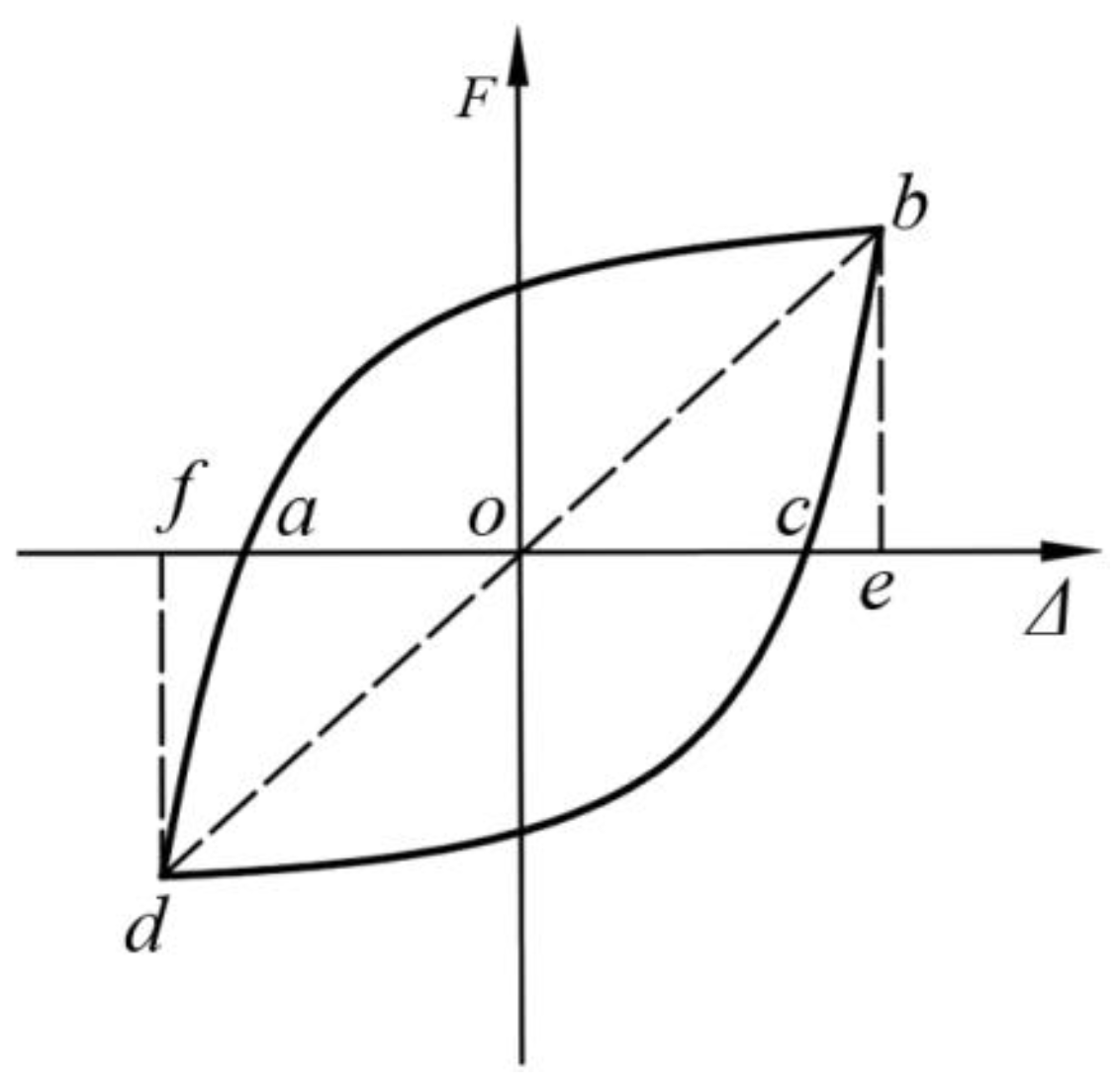
4.7. Energy Dissipation

As illustrated in Figure 16, the area (S_abc + S_cda) enclosed by the load-drift hysteretic loop formed by segments ab, bc, cd, and da is related to the amount of energy dissipated. The energy dissipation factor (h_e), commonly used to represent the energy dissipation capacity of a structure, is defined in Equation (5). The parameter (S_obe + S_odf) in Equation (5) refers to the area enclosed by the curves ob, be, eo, od, df, and fo.

$$h_e={\displaystyle \frac{1}{2\pi }}.{\displaystyle \frac{S_{abc}+S_{cda}}{S_{obe}+S_{odf}}},$$

(5)

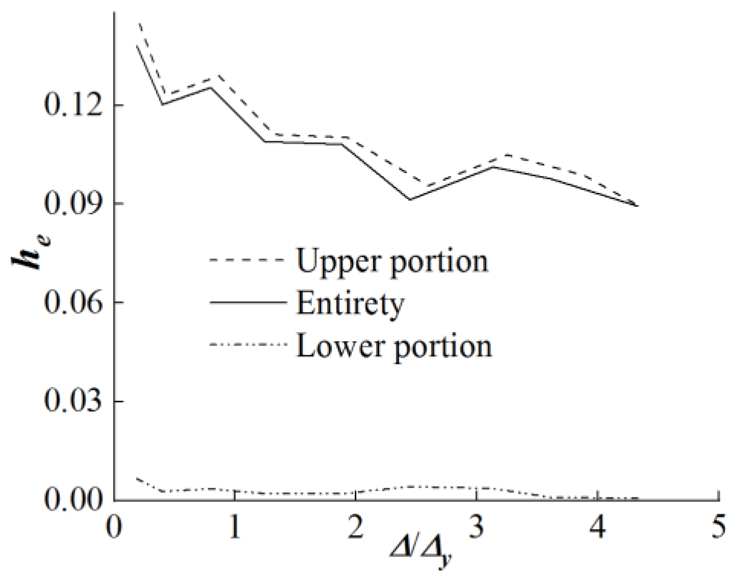
Figure 17 presents the energy dissipation factor for the entire specimen, along with its upper and lower portions. The graph indicates that the energy dissipation factor for the entire specimen decreases from 0.138 to 0.089 as the ductility ratio increases. In contrast, the energy dissipation factor for the upper portion decreases from 0.145 to 0.09, remaining higher than that of the entire specimen. Meanwhile, the energy dissipation factor for the lower portion shows relatively low values, fluctuating between 0.007 and 0.001 as the ductility ratio increases. This suggests that in the confined high AAC panel wall with a door frame in its lower portion, energy is primarily dissipated through the relatively weaker upper portion.

4.8. Shear Angle

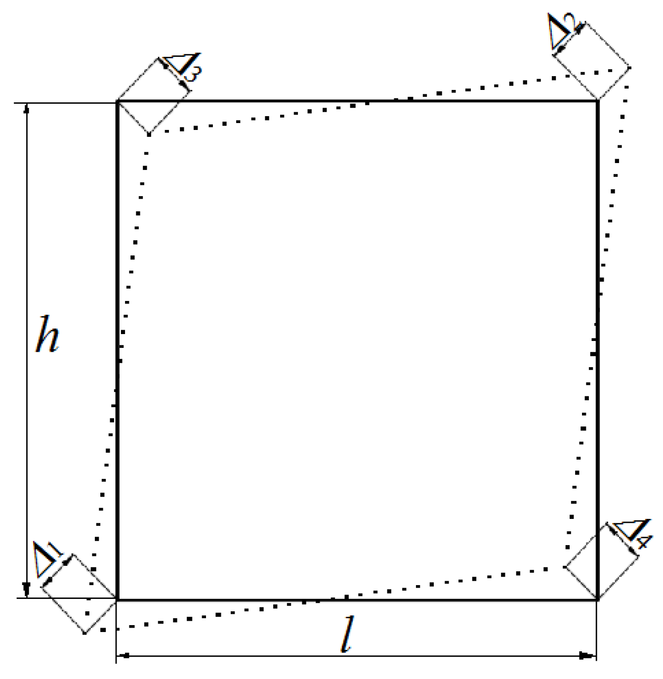
When shear deformation occurs in a rectangular structure, a schematic diagram for calculating the shear angle is presented in Figure 18. In Figure 18, where l and h represent the horizontal length and vertical height of the structure before deformation, respectively, Δ₁, Δ₂, Δ₃, and Δ₄ correspond to the distances between various corners before and after deformation [16]. The shear angle (γ) is determined by Equation (6). By setting Δ₁ and Δ₄ to zero, Equation (7), for calculating the shear angle of the structure with a fixed base, can be obtained.

$$\gamma ={\displaystyle \frac{\sqrt{l^2+h^2}}{2lh}}({\Delta }_1+{\Delta }_2+{\Delta }_3+{\Delta }_4)$$

(6)

$$\gamma ={\displaystyle \frac{\sqrt{l^2+h^2}}{2lh}}({\Delta }_2+{\Delta }_3)$$

(7)

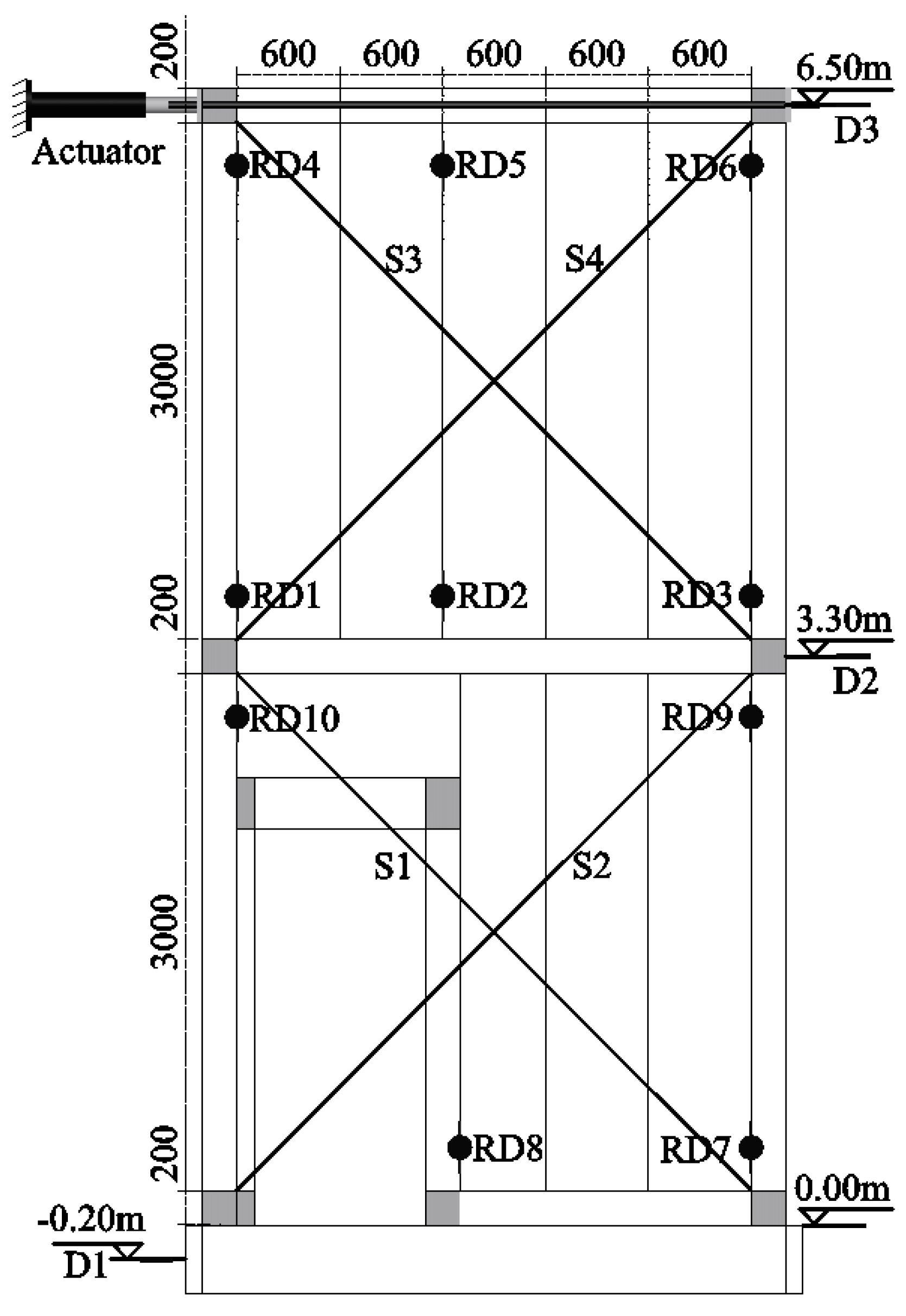
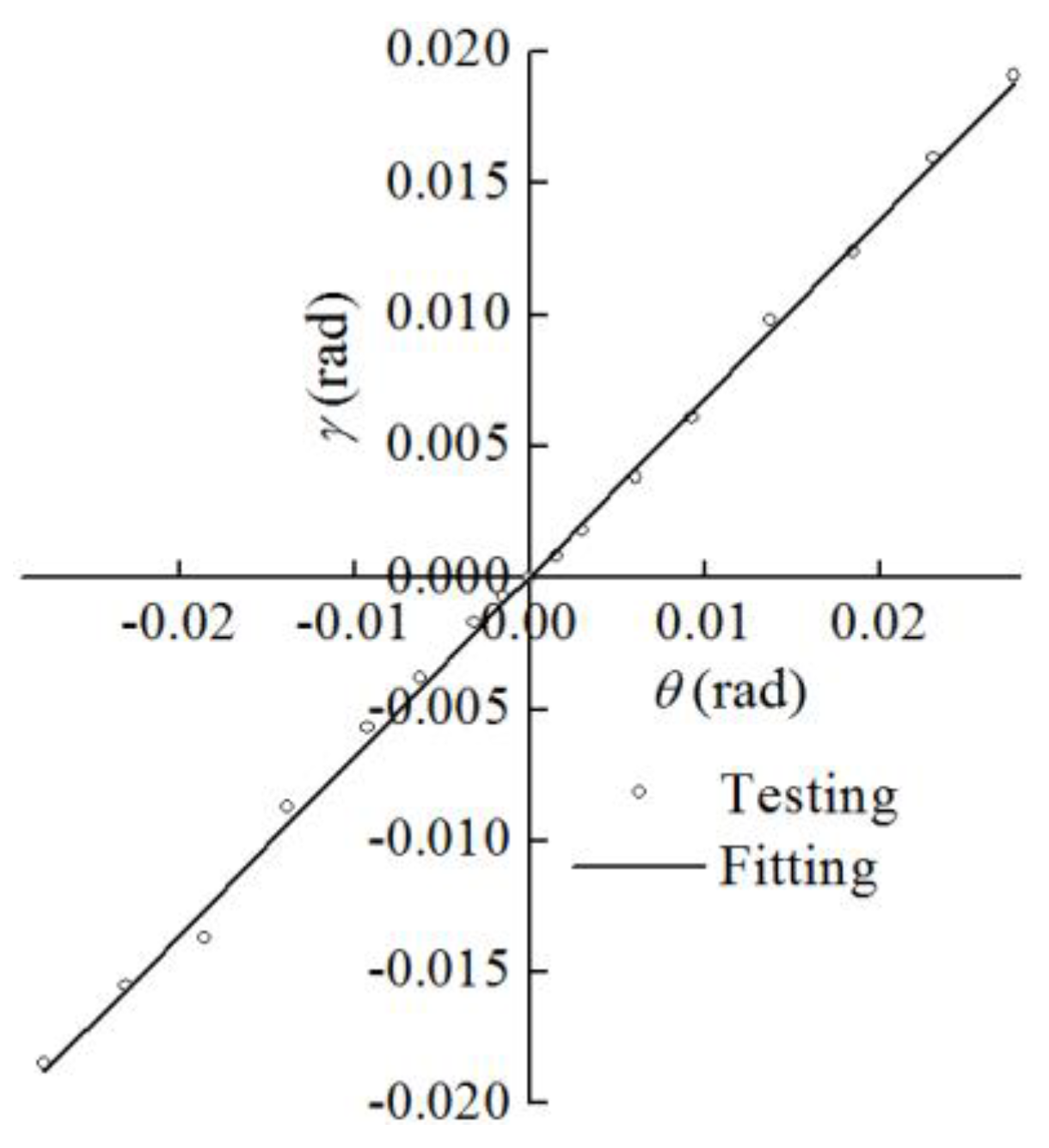
As illustrated in Figure 5, diagonal displacements of the lower (upper) portion of the specimen are measured using wire displacement gauges S1 (or S3) and S2 (or S4). Figure 19 illustrates that the shear angle (γ) increases almost linearly with the inter-story drift rotation (θ). After fitting the data from the tested benchmark to a linear function model (Equation (8)), the fitted parameter is 0.68, indicating a strong correlation coefficient (R² = 0.99). The fitted curve is also presented in Figure 19.

$$\gamma =0.68\theta$$

(8)

4.9. Relative Slippage

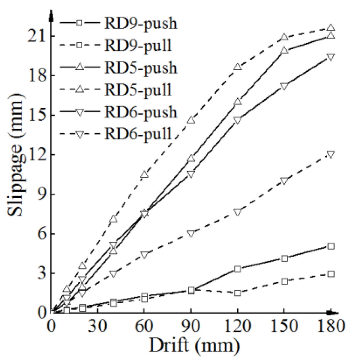
In Figure 5, the digital displacement transducer ‘RD5’ documented the slippage between the upper panels ‘P2d’ and ‘P2c’, ‘RD6’ recorded the slippage between panel ‘P2a’ and column ‘C2b’, and ‘RD9’ captured the slippage between panel ‘P1a’ and column ‘C1b’. The correlation between the component slippage and the drift of the specimen is illustrated in Figure 20. According to Figure 20, with the increase in drift, there was an increase in component slippage. Relative to the lower portion of the specimen, there was notably more slippage among the panels in the upper portion, signifying that deformation was predominantly concentrated in the upper portion of the specimen.

Within the upper portion, the slippage of the side panels was less than that of the middle panels, indicating a gradual reduction in the confining effect of the top beam ‘B2f’ on the panels from the side toward the middle. In the case of the central panel, the slippage remained comparable in both push and pull directions. Conversely, for the side panel ‘P2a’, slippage was smaller in the pull direction, highlighting a heightened interaction between the upper right corner of panel ‘P2a’ and joint ‘J5’ of the confining frame when subjected to pulling forces.

4.10. Strains of Reinforcements

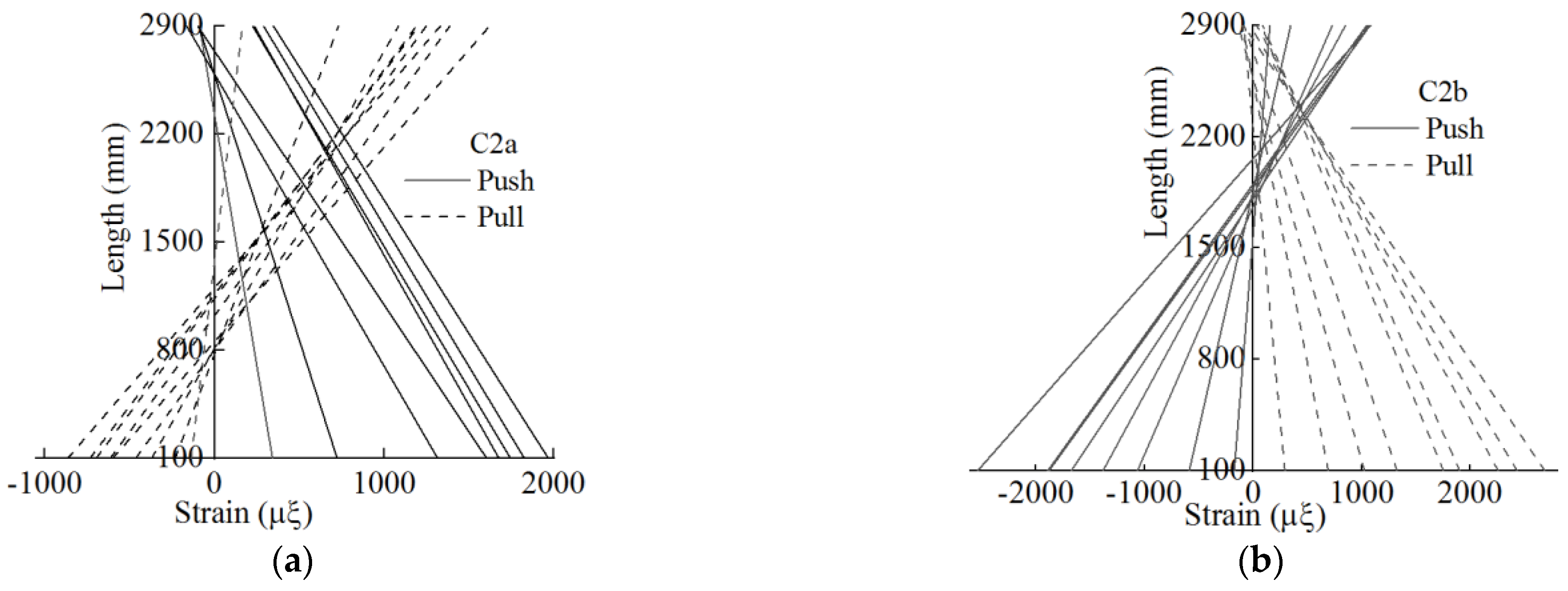
In Figure 5, strain gauges were positioned at the intended points of the longitudinal reinforcements within the left column ‘C2a’ and the right column ‘C2b’ of the upper portion of the specimen. The spacing from the strain gauges to the ends of the columns was set at 50 mm, with a distance of 2900 mm between the strain gauges. As the drift increased, the resulting strains in the column reinforcements are depicted in Figure 21. On the graph, the horizontal axis illustrates the strain in the longitudinal reinforcements, while the vertical axis represents the distance between the strain gauges.

When the drift was 60 mm or less, the majority of steel reinforcements in the left column ‘C2a’ under push loading and in the right column ‘C2b’ under pull loading experienced tensile forces. flexural points were evident in the column, situated within the upper 1/4 of the column height, with tensioned reinforcements extending through the lower 3/4 of the column height. However, when the drift reached 60 mm, both the left column ‘C2a’ under push loading and the right column ‘C2b’ under pull loading exhibited tension in all steel reinforcements across the entire column height, eliminating the presence of any flexural points.

In the pull direction, a flexural point was present in the left column ‘C2a’, while in the push direction, a flexural point occurred in the right column ‘C2b’. The flexural point in the left column ‘C2a’ was positioned within 1/2–3/4 of the column height from the top, featuring a longer length of tensioned reinforcements. Conversely, the right column ‘C2b’ exhibited a flexural point within 1/4–1/2 of the column height from the top, with a shorter length of tensioned reinforcements.

Owing to the diagonal strut effect induced by the panels, the left column in the push direction and the right column in the pull direction experienced predominant tension forces and bending moments. Conversely, the right column in the push direction and the left column in the pull direction were subjected to bending moments. Considering the potential lack of symmetry in the panel arrangement during construction, the positions of the flexural points could vary within the middle region of the column.

4.11. Initial Stiffness of Confined High AAC Panel Walls

The calculation diagram for the confining frame is shown in Figure 22. As shown in Figure 22, two hinged rods are placed on either side of the top of the door opening, connecting the door frame to the confining frame. The lateral stiffness of the confining frame is determined using the D-value method [24].

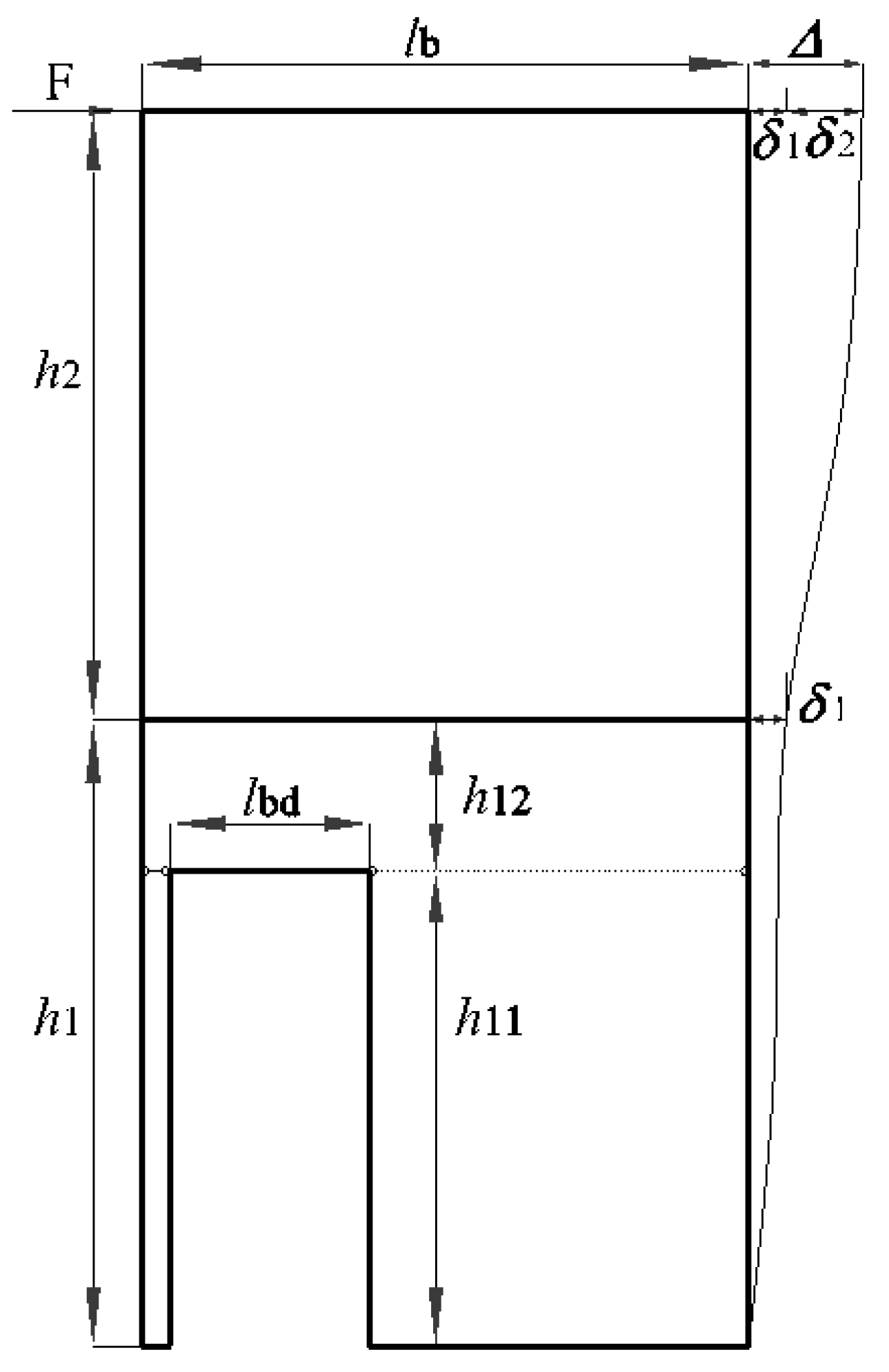
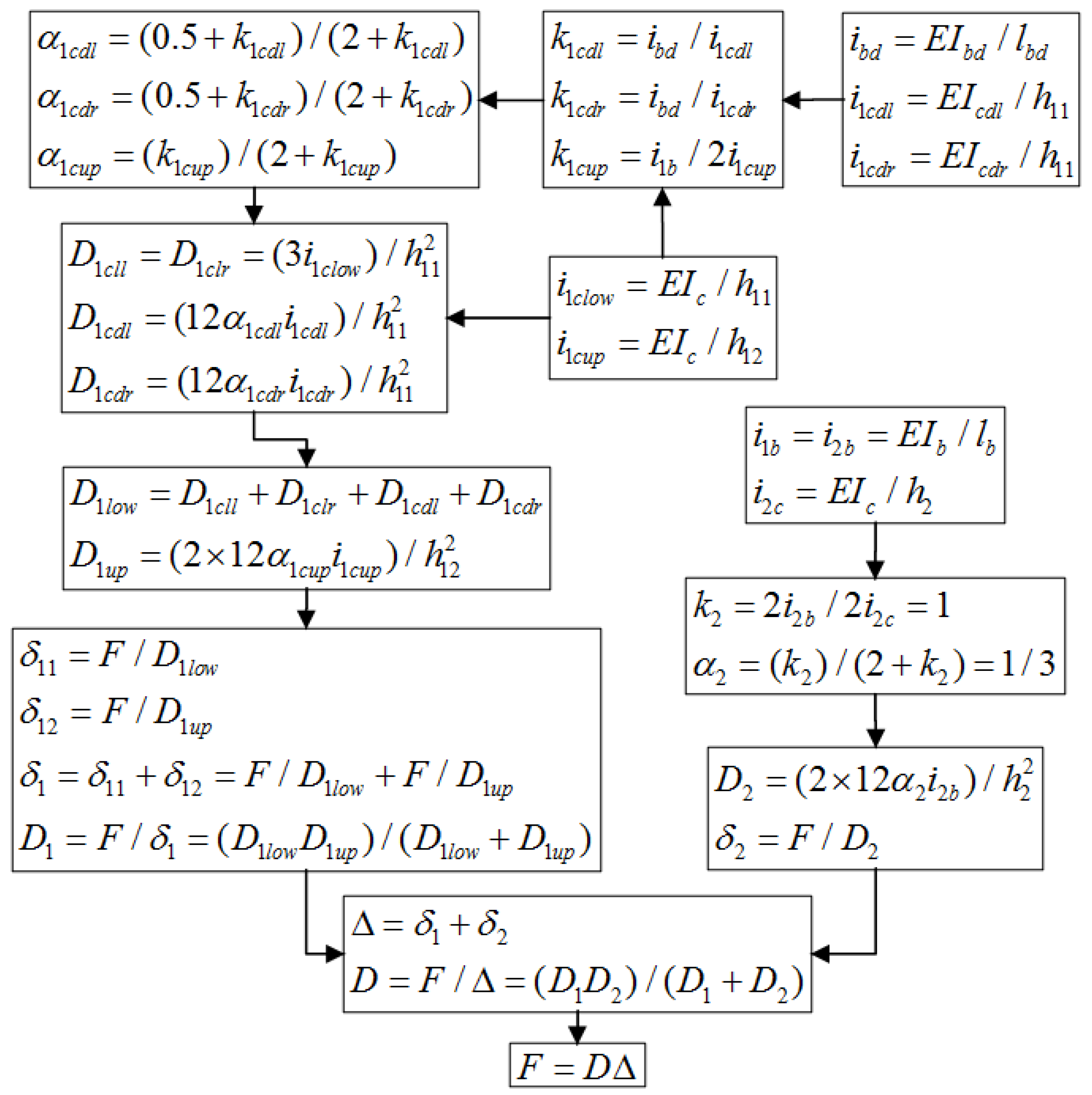
The calculation process for determining the lateral stiffness is illustrated in Figure 23. As shown in Figure 23, Δ represents the drift of the specimen at the top. The lateral stiffness values, D, D₁, and D₂, correspond to the entirety, lower portion, and upper portion, respectively. The drifts of different parts at heights h₁, h₂, h₁₁, and h₁₂ of the confining frame are denoted as δ₁, δ₂, δ₁₁, and δ₁₂, respectively. The lateral stiffness values D_1low and D_1up pertain to the parts at the heights h₁₁ and h₁₂ of the confining frame. The symbol D_1cll represents the lateral stiffness of the left column at height h₁₁, while D_1clr denotes the lateral stiffness of the right column at the same height. D_1cdl indicates the stiffness of the left column of the door frame, and D_1cdr represents the stiffness of the right column. E refers to the modulus of elasticity of concrete. I_bd is the moment of inertia of the beam, I_cdl is the moment of inertia of the left column of the door frame, and I_cdr is the moment of inertia of the right column of the door frame. Additionally, I_b and I_c represent the moments of inertia of the beam and column of the confining frame, respectively. The dimensions of the precast members and the modulus of elasticity can be found in Table 1 and Table 2.

The stiffness of the lower portion, upper portion, and confining frame was calculated using the D-value method. The results of these calculations and tests are presented in

Table 8. Calculated initial stiffness.

	Dave (kN/m)	Dcal (kN/m)	Error (%)
Entirety	980	1004	2.48
Upper portion	1270	1375	8.27
Lower portion	4285	3722	−13.13

. In Table 8, the symbol D_ave represents the stiffness obtained by averaging the positive and negative stiffness values obtained from the tests, while D_cal denotes the calculated stiffness. As shown in Table 8, the calculated stiffness for the entire confining frame using the D-value method closely matches the experimental results, with only a 2.48% deviation from the average experimental stiffness. The errors in the calculated stiffness for the lower and upper portions are 8.27% and 13.13%, respectively. These errors are relatively small, indicating that the D-value method is suitable for calculating the initial stiffness of confined high AAC panel walls.

4.12. Load-Bearing Capacity of Confined High AAC Panel Walls

For high AAC walls with upper and lower portions, the confining frame tends to fail in the portion with fewer columns. Therefore, this portion can be selected as the sub-structure for calculating the load-bearing capacity of the confined high AAC panel walls. In this study, the upper portion of the confining frame, which has two columns—fewer than the lower portion—was chosen as the sub-structure for the calculation.

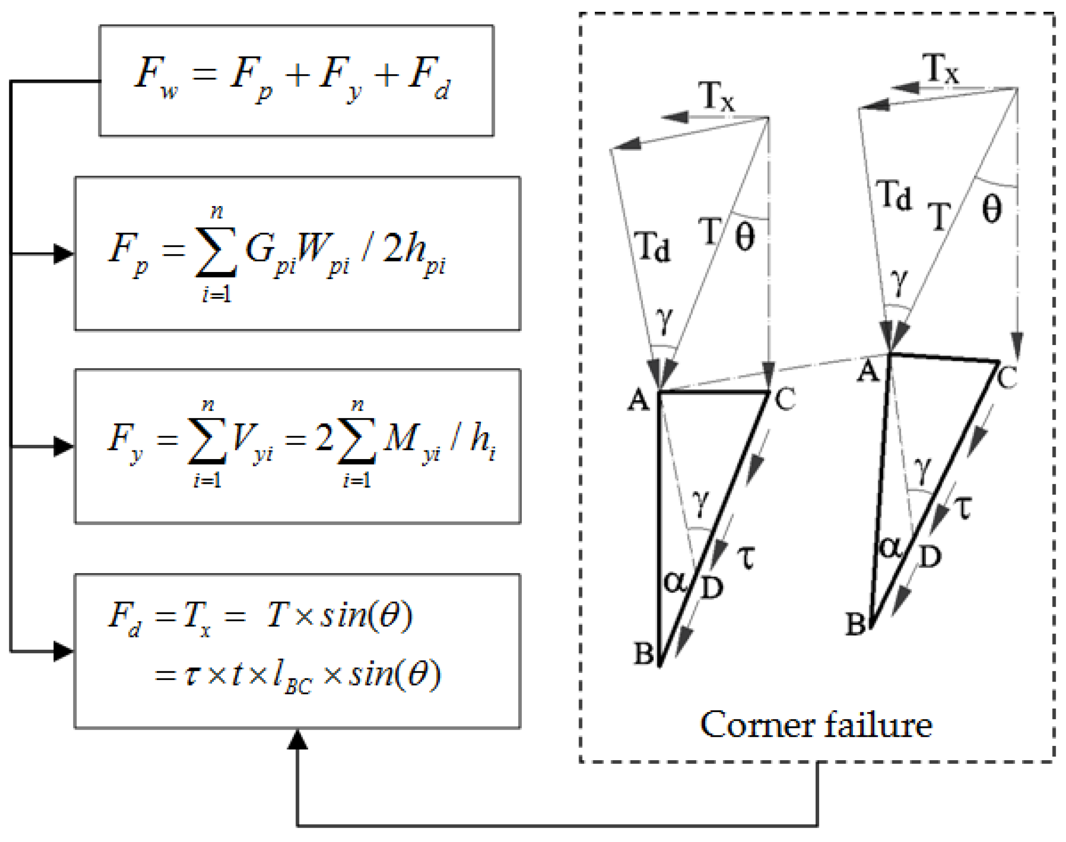
The calculation process [16] for the load-bearing capacity of the sub-structure is illustrated in Figure 24. In this figure, the symbol F_p represents the horizontal force used to counteract the weight of the plates during rotation. Additionally, F_y indicates the horizontal yielding force of the sub-structure, while F_d denotes the horizontal force that leads to the failure of the diagonal brace. The self-weight G_pi of panel i can be calculated using the formula G_pi = V_pi × ρ, where ρ is the bulk density of AAC and V_pi is the volume of panel i. The symbol W_pi represents the width of panel i. The symbol V_yi indicates the yielding shear force in the sub-structure, and the symbol h_i is the length of the columns.

The yielding moment of the confining beams, denoted as M_y, can be calculated using Equation (9). In this equation, f_y represents the yield strength of the rebar, and A_s is the cross-sectional area of the rebar. The symbol a_s′ denotes the distance from the centroid of the compression rebar to the compressive edge of the cross-section, while h₀ represents the effective height of the cross-section.

$$M_y=f_y{A}_s(h_0-a_s^{\prime })$$

(9)

The diagram of the diagonal strut is illustrated in Figure 10. Taking the corner P_c (shown in Figure 10) as an example, shear failure at the corner is depicted in Figure 24. According to phenomenon obtained from literature [16] and the experiments conducted in this study, the failure of the corners of panels in confined AAC structures does not occur simultaneously. Instead, it occurs sequentially with increasing drift, beginning with the side panels and followed by the center panels. Therefore, the diagonal strut effect of AAC panels can be calculated using the single brace model (as shown in Figure 24). In Figure 24, in the equation used to calculate the horizontal force that causes failure of AAC panels, the symbol l_BC represents the length of the side BC, t denotes the thickness of AAC panels, and τ refers to the shear strength of autoclaved aerated concrete, which can be considered equivalent to its tensile strength.

In the case of the autoclaved aerated concrete used in this study, the shear strength τ is 0.5 Mpa, and the thickness t is 200 mm (as shown in Table 1 and Table 2). When the angle θ is within the range of 0–5 °C, using F_d = 11.08 kN will not introduce significant error [16].

Based on the calculation process outlined in Figure 24, the forces F_y, F_d, F_p, and the load-bearing capacity of the sub-structure F_w are calculated and presented in

Table 9. Load-bearing capacity.

Fy	Fd	Fp	Fw	Fave	Error %
(kN)	(kN)	(kN)	(kN)	(kN)
15.88	11.08	5 × 0.288 = 1.44	28.40	27.23	4.30

. As shown in Table 9, the calculated load-bearing capacity is very close to the average value obtained from experimental positive and negative peak loads, with an error of only 4.30%. This indicates that the method proposed in this study for calculating confined high AAC panel walls is feasible.

5. Conclusions

In this study, a full-scale confined high AAC panel wall was fabricated and tested. Its seismic performance was evaluated through both experimental and theoretical methods. The conclusions are summarized as follows:

• Due to enhanced stiffness and lateral load-carrying capacity provided by the door frame in the lower portion, deformation and failure primarily concentrated in the upper portion of the specimen. The drift of the upper portion constitutes 76.94–83.63% of the entire drift at each intended drift. The energy dissipation factor for the upper portion of the specimen is 0.8–4.8% greater than that of the entire specimen. The energy dissipation factor of its upper portion is 0.8–4.8% higher than that of the entire specimen. The strength degradation factor of the confined high AAC panel walls ranges from 0.971 to 0.716.
• Shear failure occurred at the joints of the confining frame and at the corners of the AAC panels. Flexural cracks developed in the columns of the upper portion of the confined high AAC panel walls, and the top beam exhibited upward bending and developed vertical flexural cracks.
• Confined panel walls retained a strong load-bearing capacity even after the failure of the confining frame, and the infill AAC panels contributed to the ductility and deformation capacity of the confined high AAC panel wall system.
• The confined high panel walls demonstrated inter-story drift rotation capacity that meets the requirements of the Chinese code, allowing them to remain stable and secure even before the main frame structure fails.
• There was a 20 mm gap between the panels and the confining frame at both sides and the top. Initially, with drifts less than 20 mm, the confining frame primarily carried the lateral load. However, as the drift increased from 40 mm to 90 mm, the diagonal strut effect of the AAC panels became more pronounced. Following the peak load, the confining frame developed ‘joint hinges’, leading to a reduction in its lateral-load resistance. Consequently, the confined AAC panel wall primarily depended on the AAC panels to withstand lateral loads.
• The calculated stiffness for the confining frame using the D-value method closely aligns with experimental results, exhibiting only a 2.48% deviation from the average experimental stiffness. The calculated load-bearing capacity deviates from the experimental average by only 4.30%.