Bi-Level Design Optimization for Demand-Side Interval Temperature Control in District Heating Systems

Abstract

With China’s socio-economic growth, the demand for enhanced residential comfort in northern urban areas has surged. Traditional district heating systems often fail to meet modern users’ diverse needs, leading to inefficiencies and significant heat loss. This paper investigates optimization and transformation methods for demand-side-oriented heating systems. We propose key design parameters that facilitate a shift from source-end to demand-end dominance and develop a bi-level planning model for operational scheduling. The model integrates building thermal storage and adjustable user temperature ranges to optimize multi-thermal source systems. Key contributions include identifying critical renovation parameters and establishing the relationship between temperature control range and system capacity. Results demonstrate that the optimized system provides interval temperature control for 96.02% of the heating season and increases the full-load duration ratio of heat source equipment by 29.54% compared to traditional systems. These improvements enhance operational efficiency, reduce heat loss, and better align heating provision with users’ dynamic thermal demands. This research offers a robust theoretical foundation and practical guidelines for transitioning to demand-end dominated district heating systems, contributing to more sustainable and responsive heating solutions.

1. Introduction

As China’s socio-economic status continues to rise, the living standards of its citizens have shown a corresponding upward trajectory, accompanied by escalating demands for enhanced living comfort. Within this context, district heating, which serves as a cornerstone of living quality for residents in northern urban locales, finds it increasingly challenging to cater to the differentiated needs of contemporary users via its traditional source-controlled and uniform supply approach. Due to the absence of thermal regulation capabilities at the user end of current heating systems, numerous consumers find themselves compelled to open windows as a means of reducing indoor temperatures. Studies have demonstrated that this practice can result in heat losses amounting to as much as 23% of total heat consumption [1]. Concurrently, in line with the “Dual Carbon” strategy advanced by the Chinese government, an increasing number of clean energy sources are being integrated into district heating systems, with the aim of diminishing carbon emissions and enhancing the efficiency of heat provision. As the demand for differentiated control increases on the demand side, coupled with the increasing inclusion of intermittent clean heat sources, the flexibility of traditional heating systems is revealed to be limited. There exists a pressing need for system design and operational modifications to foster a demand-driven reshaping of heating systems and the efficient integration of clean heat sources [2].

In terms of design, the fourth and fifth generations of district heating and cooling systems have delineated the current developmental trajectory for regional heating systems, with a focus on harnessing the potential of energy use on the demand side [3,4]. Contemporary research predominantly centers on the assessment and implementation methodologies for demand-side response [5,6,7,8,9]. Coss [10] developed a multi-objective optimization model for heating systems, which is based on heat load characterization and aims to evaluate the applicability of demand-side management technologies within district heating systems. Saletti [11] constructed a grey-box control model for large district heating systems to facilitate real-time optimization and predictive control. The model has shown significant potential in applying demand-side management. Yin [12] established a novel demand-side response estimation framework for residential and commercial buildings, validated by a combination of EnergyPlus and dual-mode models, demonstrating that the framework accurately predicts demand-side responses with an accuracy of 80% to 90%. Other related studies have focused on research into user load response influenced by different time-of-use pricing [13,14,15,16] and on envelope retrofitting driven by demand-side management [17,18].

Within the domain of operational control, current studies focus primarily on operational scheduling at the energy source side of systems. This includes joint dispatch optimization focusing on cogeneration units [19,20,21,22,23] and strategies to increase the share of renewable energy in system operations [24,25,26,27,28]. With the growing emphasis on a demand-driven approach, more scholars are focusing on the critical role of building thermal storage in the operation of heating systems. Turski [29] assessed buildings and heating networks’ function as thermal energy storage (TES) devices within district heating systems. Li [30] analyzed building thermal storage’s significance for heating systems, summarizing TES technologies by their type, application, and scope. Dominković [31] developed a simulation model for building flexibility, integrated with district heating systems, to study buildings’ energy storage potential. Kensby [28] conducted pilot tests on five multi-family residential buildings to investigate heating systems’ flexibility under varied heating and cooling cycle durations. Kensby’s [32] subsequent papers evaluated differences in control between building thermal storage and centralized thermal storage tanks. Research in reference [33] calculated low-energy buildings’ thermal storage potential within heating systems, indicating these buildings can maintain autonomy for several hours during the storage process. The buildings’ adjustable temperature range significantly impacts autonomy duration.

In research into the demand side of district heating systems, it has been widely assumed by scholars that the thermal source capacity is sufficient to cater to various demand scenarios at the user end. However, several critical gaps persist in the current body of knowledge:

(1)

Conventional Design Limitations in China’s District Heating Market: In the context of China’s district heating market, the conventional design process remains largely source-oriented, predicated on the assumption that the demand-side temperature remains constant and that the magnitude of the heat load is primarily influenced by outdoor temperatures. This source-centric approach overlooks the dynamic and variable temperature needs of users, which can lead to mismatches between supply and demand.

(2)

Insufficient Capacity Under Demand-Driven Approaches: Under a demand-driven approach, users’ temperature needs span a specific range, potentially leading to instances where the existing thermal source capacity is insufficient to meet the heat demands. There is a lack of comprehensive studies addressing how fluctuating user temperature requirements impact the adequacy of thermal source capacities, especially during peak demand periods or extended cold spells.

(3)

Lack of Methodologies for Capacity Expansion Determination: The relationship between the demand side’s temperature control range and the thermal source equipment’s capacity, along with the method for determining the necessity of thermal source expansion in demand-driven scenarios, remains an open question in current research. Existing models do not adequately provide frameworks for assessing when and how to expand thermal source capacities in response to variable demand-side conditions.

(4)

Integration of Building Thermal Storage in Operational Control: In the realm of heating system operational control, research increasingly centers on quantifying buildings’ thermal storage capacity and its impact on the internal thermal environment, particularly when buildings act as thermal storage units. However, the interplay between building thermal storage capacity and the adjustable temperature range at the user end during system operation is not well-understood, highlighting a need for solutions that enhance operational control by leveraging thermal storage effectively.

Addressing these gaps, this study thoroughly examines the correlation between the capacity of thermal sources and the temperature control range on the demand side during the modernization of traditional heating systems. It further develops a bi-level planning model that incorporates changes in building thermal storage and the user’s adjustable temperature range to guide the operational scheduling of multi-thermal source heating systems post-renovation. The main contributions of this work are summarized as follows:

(1)

In the context of optimizing traditional heating systems, the study clearly delineates the specific design and renovation process, identifying key design parameters and their calculation methods during the renovation. This elucidation clarifies the relationship between the temperature control range on the demand side and the system’s thermal source capacity, aiming to mitigate operational conflicts between the supply and demand sides. This clarity is particularly critical for the optimization and renovation of heating systems.

(2)

A novel bi-level operational scheduling model has been developed for heating systems post-optimization. This model, in determining operational schedules, considers both the thermal efficiency of various heat source equipment and the significant impact of system thermal storage on the adjustable temperature range for end-users. This ensures that the system optimally balances economic and carbon emission considerations while meeting the temperature control needs of demand-side users.

This paper is organized as follows: Section 2 explores the optimization and renovation processes of traditional heating systems, elucidating the definition and calculation methodologies of key design parameters. Section 3 introduces the methodology behind constructing the bi-level operational scheduling model. Section 4 presents a detailed case study, followed by a discussion. Finally, Section 5 summarizes the principal findings and provides insights into future prospects.

2. Design Method

2.1. System Improvement Process

A typical heating system consists of three main components: the heat source, the heating network, and the heating buildings (or heat users), as shown in Figure 1. The heat source is responsible for producing thermal energy, often through multiple heat generation devices. The heating network serves as the distribution system, carrying thermal energy via heat carriers to the heating buildings, where it is consumed. Traditional heating systems generally follow a supply-centric approach, where heat is distributed to users based on a uniform temperature demand. This approach, however, does not account for individualized temperature needs and relies on source-end control, which can lead to inefficiencies and user discomfort.

As demands for improved living conditions and more precise temperature control increase, it has become necessary to transform traditional heating systems. A shift from source-end dominance to demand-side regulation is essential to meet the diverse heating needs of users while improving system efficiency. The process of optimizing and retrofitting traditional heating systems to incorporate demand-side regulation is shown in Figure 2.

The specific process is as follows:

(1)

Categorization of users: Users on the demand side of the original secondary network heating system are categorized based on their heating characteristics into general users, flexible load users, and interval temperature control users. This categorization requires a clear understanding of the proportion of the load each type of user contributes to in the original heating system.

(2)

Calculation and selection of the adjustable temperature range: First, the maximum controllable temperature difference achievable by the buildings of interval temperature control users is calculated. An appropriate temperature range is then selected as the adjustable temperature range for these users.

(3)

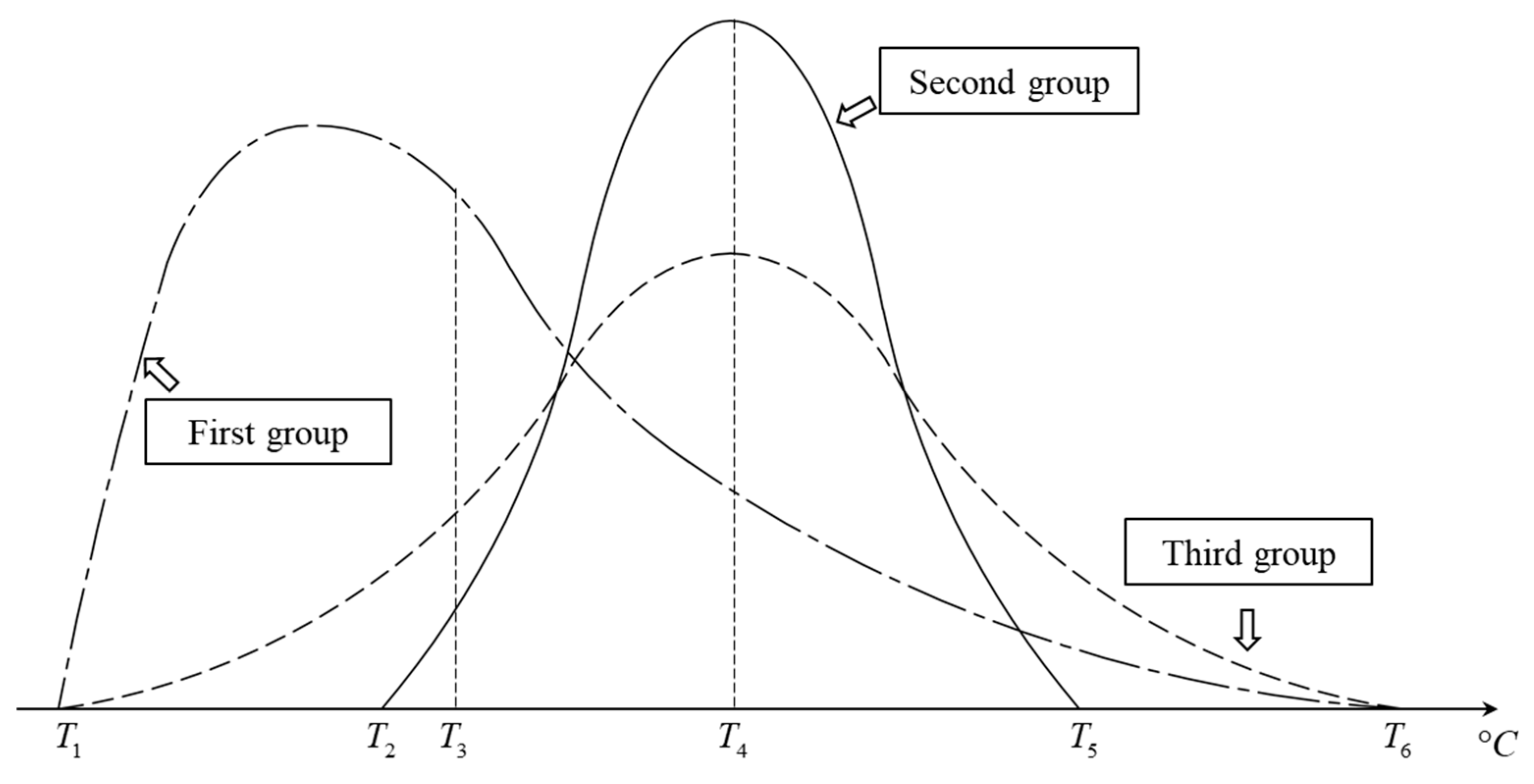
Determination of the interval temperature distribution: The overall temperature control distribution for the demand-side control users is established using empirical analysis or surveys.

(4)

Decision on heat source expansion: Based on the load proportion of demand-side control users, the adjustable temperature range, and the corresponding temperature distribution, the duration for which the heat source system can accommodate interval temperature control during the heating season is calculated. This calculation determines whether the heat source needs to be expanded.

(5)

Heat source expansion: If expansion of the original heat source is necessary, the required expansion capacity is calculated, followed by the selection and installation of a new heat source. Finally, necessary control and sensing facilities are installed, completing the transformation of the existing heating system into a flexible, smart heating system. If the original heat source does not require expansion, the necessary control and sensing facilities are installed directly.

In the aforementioned process, general users are defined as those with constant temperature needs, who are supplied with sufficient heat based on these requirements. This category mainly comprises buildings such as hospitals and hotels, along with production buildings with constant temperature requirements. Flexible load users are characterized by a variable heat load and have relatively lower requirements for building comfort, which permits some temperature fluctuation within the building. These users engage in the operation and control of the entire heating system as flexible loads, playing a crucial role in “peak shaving and valley filling,” which is vital for flexible scheduling. Commercial buildings and universities are often categorized as major flexible load users. Interval temperature control users possess a significant level of autonomous temperature control. Primarily comprising residential building users, they serve as the main agents of demand-side control. Unlike general and flexible load users, these users are billed by household, and the system needs the capability for demand-side control to satisfy the individual heating needs of residential users.

In the comprehensive transformation process, the concept of “Determine the Interval Temperature Distribution” signifies a critical difference between traditional heating systems before and after renovation. “Whether the Heat Source is Expanded” and “Calculating Expansion Capacity” constitute key steps in the transformation process.

2.2. Distribution of Adjustable Temperature Intervals

In the optimized and remodeled heating system, the configuration includes general users, flexible load users, and interval temperature control users. For general users, the heat load remains consistent with that of similar buildings in the original traditional system. Although flexible load users serve as thermal storage entities, performing specific heat storage and release control tasks, their heat load does not change compared to the original system. Thus, the variance in heat loads between the two systems primarily arises from the interval temperature control users.

Interval temperature control users utilize a segmented rather than a uniform approach to temperature adjustment. The designed heat load size is influenced not only by the range of temperatures to which users can adjust, but also by the temperature distribution within that range. Figure 3 illustrates the adjustable temperature ranges and their corresponding temperature distributions for three groups of interval temperature control users of identical scale. As depicted, although the second and third groups of users possess different adjustable temperature ranges, they share the same mean temperature, resulting in identical heat loads. Conversely, the first and third groups have the same adjustable temperature range, but their distribution means differ, leading to distinct heat load sizes.

In the optimization process of traditional heating systems, the feasible range of temperature control and its corresponding temperature distribution serve as the basis for calculating the design heat load of the heating system. The size of the achievable temperature control range is determined by the physical characteristics of the buildings in the area, while the temperature distribution necessitates extensive surveys or analysis of historical data. In this paper, the focus is on the selection of heat source expansion and system operational control, leading to the assumption that the temperature distribution among interval temperature control users exhibits a symmetrical distribution around the mean value within the control range. The designed heat load for interval temperature control users is calculated based on the mean temperature distribution within the adjustable range, using the original design heat load of the residential buildings as the foundation. The mean temperature distribution within the adjustable range is regarded as the indoor design temperature for interval temperature control users, and the formula for calculating the design heat load is as follows:

$$Q_{DSU}^{\prime }={\displaystyle \frac{T_n^{\prime }-T_w^{\prime }}{T_n^{\prime }-T_w^{\prime }}}\cdot Q_{resident}^{\prime }$$

(1)

where $Q_{DSU}^{\prime }$ represents the designed heat load for users with interval temperature control (MW). ${\overline{T}}_n^{\prime }$ denotes the average temperature (°C), within the adjustable temperature range. $T_w^{\prime }$ stands for the calculated outdoor temperature during winter in the heating area (°C). $T_n^{\prime }$ represents the designed indoor temperature (°C), specifically for residential building users. $Q_{resident}^{\prime }$ refers to the designed heat load for residential users when considered within traditional heating systems (MW).

2.3. Calculation Method of Heat Source

In comparison to traditional heating systems, the difference in heat load for optimized and retrofitted systems arises from users’ ability to control the temperature within a specified range. When the average temperature within the adjustable range exceeds the original indoor design temperature, the heat source of the original system fails to meet the thermal demand according to its designed capacity. However, during the heating season, the period in which outdoor temperatures fall below the calculated outdoor temperature is relatively brief, with outdoor temperatures remaining above the calculated values for most of the period. Therefore, the decision to expand the system’s heat source capacity during retrofitting should be based on whether the original system’s heat source can meet the users’ design demand throughout the required period. If the original system’s heat source capacity remains unchanged and users’ control requirements are unmet for only a brief period, then expanding the heat source capacity is unnecessary. Conversely, if users cannot meet their control requirements for an extended period, heat source expansion becomes necessary.

Thus, in the optimization and retrofitting of traditional heating systems, the decision to expand the heat source capacity involves four key design parameters: incremental design heat load, critical outdoor temperature, the ratio of the design interval continuation time, and the effective adjustable temperature range. The incremental design heat load measures the degree of variation in system load, indicating the required magnitude of heat source expansion during system augmentation. The critical outdoor temperature is a pivotal parameter in the optimization and retrofit design process, helping calculate other key parameters. The ratio of the design interval continuation time serves as a key indicator for system expansion, determining whether the optimized retrofit system needs augmentation. The effective adjustable temperature range represents the actual scope for adjusting the system’s interval temperatures for users under various conditions, reflecting the overall comfort level of this user group.

2.3.1. Incremental Design Heat Load and Critical Outdoor Temperature

In an existing heating system servicing residential buildings, several interrelated dynamics are observed.

$$Q_{resident}^{\prime }=\xi Q_{gross}^{\prime }$$

(2)

where $\xi$ represents the proportion of residential buildings within the overall heating system ($\xi \in \left(0,1\right]$); $Q_{gross}^{\prime }$ refers to the total design heat load (MW) of traditional heating systems; When outdoor temperatures diverge from the designated conditions, the heat load of the traditional heating system exhibits the following relationship with the design heat load:

$$Q_{gross}={\displaystyle \frac{T_n^{\prime }-T_w}{T_n^{\prime }-T_w^{\prime }}}\cdot Q_{gross}^{\prime }$$

(3)

where $Q_{gross}$ represents the total heat load under non-design conditions for the traditional heating system (MW); $T_w$ stands for the outdoor temperature at a given time during the heating season within the heated area (°C). Consequently, under outdoor temperatures that exceed design conditions, the traditional heating system’s heat source offers additional heating capacity as described by the following equation:

$$\Delta Q_{gross}=Q_{gross}^{\prime }-Q_{gross}={\displaystyle \frac{T_w-T_w^{\prime }}{T_n^{\prime }-T_w^{\prime }}}\cdot Q_{gross}^{\prime }$$

(4)

After optimizing the traditional heating system, variations in the system’s heat load arise from interval temperature control users. Compared to the conventional system, the calculation method for the incremental heat load of the optimized heating system is delineated below:

$$Q_{increment}=Q_{DSU}-Q_{resident}$$

(5)

$$Q_{DSU}={\displaystyle \frac{{\overline{T}}_n^{\prime }-T_w}{{\overline{T}}_n^{\prime }-T_w^{\prime }}}\cdot Q_{DSU}^{\prime }$$

(6)

$$Q_{resident}={\displaystyle \frac{T_n^{\prime }-T_w}{T_n^{\prime }-T_w^{\prime }}}\cdot Q_{resident}^{\prime }$$

(7)

After substituting the Formulas (1), (2), (6), (7) into (5), we obtain:

$$Q_{increment}={\displaystyle \frac{{\overline{T}}_n^{\prime }-T_n^{\prime }}{T_n^{\prime }-T_w^{\prime }}}\cdot \xi Q_{gross}^{\prime }$$

(8)

where $\Delta Q_{gross}$ represents the additional heating capacity that the heat source can provide when the outdoor temperature exceeds the design temperature during the heating season(MW); $Q_{increment}$ denotes the incremental heat load for the optimized heating system (MW); $Q_{DSU}$ stands for the heat load of interval temperature control users (MW).

Therefore, for the optimized heating system, the method for calculating the incremental heat load is presented in Equation (8). Unlike conventional heating systems, the incremental heat load of the system remains constant, depending solely on the system’s design parameters. In cases where the heat source is not expanded, only part of the thermal demand from users with interval temperature control can be met under designed conditions. During non-designed operational phases, the available heating capacity of traditional heating systems is calculated as shown in Equation (4). As outdoor temperatures rise, the heating capacity provided by the system increases. When the outdoor temperature exceeds a certain threshold, the heating capacity from the heat source will equal or exceed the incremental heat load of the optimized heating system, fully meeting the designed thermal demands of users with interval temperature control. The following relationship is thus established:

$$\Delta Q_{gross}\ge Q_{increment}$$

(9)

After substituting the Formulas (4) and (8), we obtain:

$$\left\{\begin{array}{l}{T}_w\ge T_w^{critical}\hfill \\ T_w^{critical}=\left({\overline{T}}_n^{\prime }-T_n^{\prime }\right)\cdot \xi +T_w^{\prime }\hfill \end{array}\right.$$

(10)

$$\left\{\begin{array}{l}{\overline{T}}_n\le {\overline{T}}_n^{effective}\hfill \\ {\overline{T}}_n^{effective}=\left(T_w-T_w^{\prime }\right)\cdot {\displaystyle \frac{1}{\xi }}+T_n^{\prime }\hfill \end{array}\right.$$

(11)

where $T_w^{critical}$ is defined as the critical outdoor temperature. When the outdoor temperature meets or exceeds this critical level, the designed thermal demands of users with interval temperature control are fully met during the system regulation process. ${\overline{T}}_n^{effective}$ is defined as the effective control interval average temperature. Under various outdoor temperatures, the actual average temperature within the control interval for users with interval temperature control remains below the effective control interval average temperature during the system regulation process. When the outdoor temperature drops below the calculated threshold for the heating season, the system switches to a uniform control supply mode to satisfy the basic thermal demands of the users.

2.3.2. The Ratio of the Design Interval Continuation Time and the Effective Adjustable Temperature Range

Based on the historical daily average outdoor temperature data collected from various cities over the past 30 years, a dimensionless mathematical model has been developed using mathematical analysis and regression algorithms. This model depicts the distribution pattern of outdoor temperatures during the heating season in those cities. The formula for outdoor temperature is as follows:

$$T_w=\left\{\begin{array}{cc}{T}_w^{\prime }& n_{hour}\le 120\\ T_w^{\prime }+\left(5-T_{p.j}\right)R_n^b& 120<n_{hour}\le n_{hour}^{zh}\end{array}\right.$$

(12)

$$R_n={\displaystyle \frac{n_{hour}-120}{n_{hour}^{zh}-120}}$$

(13)

$$b={\displaystyle \frac{5-\mu T_{p.j}}{\mu T_{p.j}-T_w^{\prime }}}$$

(14)

$$\mu ={\displaystyle \frac{n_{hour}^{zh}}{n_{hour}^{zh}-120}}$$

(15)

where $T_{p.j}$ represents the average temperature of the highest adjustable temperature range distribution for interval temperature control users (°$\mathrm{C}$); $R_n$ denotes a dimensionless group that indicates the duration of dimensionless continuation hours; $b$ refers to the exponent of $R_n$; $\mu$ signifies a correction factor; $n_{hour}$ represents the continuation hours (the annual average number of hours when the outdoor average daily temperature in the heating region falls to or below a certain threshold throughout the heating season); $n_{hour}^{zh}$ indicates the total duration of the heating season (h); “120” stands for the design hours not guaranteed during the heating season. In regional heating systems in China, this figure typically amounts to 120 h.

By solving Equations (10) and (12) together, a formula is derived to calculate the continuation hours during the heating season when the temperature control fails to meet the designed adjustable range, assuming the original heating system’s capacity remains unchanged.

$$n_{hour}^{unsatisfied}={\left[{\displaystyle \frac{\xi \left({\overline{T}}_n^{\prime }-T_n^{\prime }\right)}{5-T_{p.j}}}\right]}^{{\displaystyle \frac{1}{b}}}\left(n_{hour}^{zh}-120\right)+120$$

(16)

Under the conditions of the original heat source system, the duration during which the optimized heating system meets the design requirements of the adjustable temperature range for users with interval temperature control throughout the heating season is as follows:

$$n_{hour}^{satisfied}=n_{hour}^{zh}-n_{hour}^{unsatisfied}=\left\{1-{\left[{\displaystyle \frac{\xi \left({\overline{T}}_n^{\prime }-T_n^{\prime }\right)}{5-T_{p.j}}}\right]}^{{\displaystyle \frac{1}{b}}}\right\}\left(n_{hour}^{zh}-120\right)$$

(17)

$$\omega ={\displaystyle \frac{n_{hour}^{satisfied}}{n_{hour}^{zh}}}\times 100\%$$

(18)

where $n_{hour}^{unsatisfied}$ represents the number of hours during which the modified heating system unsatisfied the design requirements for the adjustable temperature range set by users with interval temperature control (h). $n_{hour}^{satisfied}$ denotes the number of hours during which the modified heating system satisfies the design requirements for the adjustable temperature range set by users with interval temperature control (h). $\omega$ represents the proportion of the heating season during which the system meets the adjustable temperature range requirements. This ratio serves as a criterion for deciding whether to expand the capacity of the heat source subsequent to the system’s optimization and modification.

In this paper, users of interval temperature control in the optimized and retrofitted heating system utilize the original indoor design temperature as the lower boundary of their adjustable temperature range. This range is defined on the assumption that the temperature distribution among users is symmetrical, centered at the mean value of the control interval. Accordingly, the adjustable temperature range for these users is specified as follows:

$$\left[T_n^{\prime },T_n^{\prime }+\Delta T\right]$$

(19)

$$\Delta T=2\left({\overline{T}}_n-T_n^{\prime }\right)$$

(20)

For a residential building that accounts for a proportion $\xi$ of the existing heating system, the original indoor design temperature is set at $T_n^{\prime }$. In the retrofitted heating system, the adjustable temperature range for interval temperature control users is $\Delta T^{\prime }$.

(1) For the optimized heating system, when $\omega \ge {\omega }_{\min }$, expansion of the heat source capacity becomes unnecessary. At this juncture, the critical outdoor temperature is determined using the following equation:

$$T_w^{critical}={\displaystyle \frac{\Delta T^{\prime }\cdot \xi }{2}}+T_w^{\prime }$$

(21)

The effective adjustable temperature range for interval temperature control users is calculated according to the following formula:

$$\Delta T^{effective}=\left\{\begin{array}{cc}\Delta T^{\prime }& T_w^{critical}\le T_w\\ \left(T_w-T_w^{\prime }\right)\cdot {\displaystyle \frac{2}{\xi }}& T_w^{\prime }<T_w<T_w^{critical}\\ 0& T_w\le T_w^{\prime }\end{array}\right.$$

(22)

Under the design conditions, the formula for expressing the duration of the heat load is as follows:

$$Q_n=\left\{\begin{array}{cc}{Q}_{gross}^{\prime }& n_{hour}\le n_{hour}^{satisfied}\\ \left(1-{\displaystyle \frac{5-T_w^{\prime }}{T_n^{\prime }-T_w^{\prime }}}\cdot R_n^b\right)\cdot Q_{gross}^{\prime }+Q_{increment}& n_{hour}^{satisfied}<n\le n_{hour}^{zh}\end{array}\right.$$

(23)

(2) After optimization of the heating system, should the condition $\omega <{\omega }_{\min }$ be met, expansion of the heat source becomes necessary. The calculation of the additional heat source capacity is delineated in Equation (8). At this juncture, the critical outdoor temperature for the system is equivalent to the calculated outdoor temperature for the heating season in the region.

$$T_{w\_KR}^{critical}=T_w^{\prime }$$

(24)

Currently, the period during which interval temperature control users can maintain conditions within the designed adjustable range is specified as follows:

$$n_{hour\_KR}^{satisfied}=n_{hour}^{zh}-120$$

(25)

The effective adjustable temperature range for interval temperature control users is calculated according to the following formula:

$$\Delta T_{KR}^{effective}=\left\{\begin{array}{cc}\Delta T^{\prime }& T_w^{\prime }\le T_w\\ \Delta T^{\prime }-2\left(T_w^{\prime }-T_w\right)& T_w^{\prime }-{\displaystyle \frac{\Delta T^{\prime }}{2}}<T_w\le T_w^{\prime }\\ 0& T_w\le T_w^{\prime }-{\displaystyle \frac{\Delta T^{\prime }}{2}}\end{array}\right.$$

(26)

An effective adjustable range of ‘0’ suggests that the heating system has achieved full load capacity under extremely low outdoor ambient temperatures, positioning the theoretical temperature for interval temperature control users at the lower limit of the adjustable range. The mathematical expression for the duration of the heat load under the designed conditions is provided below:

$$Q_n=\left\{\begin{array}{cc}{Q}_{gross}^{\prime }+Q_{increment}& n_{hour}\le 120\\ \left(1-{\displaystyle \frac{5-T_w^{\prime }}{T_n^{\prime }-T_w^{\prime }}}\cdot R_n^b\right)\cdot \left(Q_{gross}^{\prime }+Q_{increment}\right)+Q_{increment}& 120<n\le n_{hour}^{zh}\end{array}\right.$$

(27)

It should be noted that the calculations presented above are based on the most unfavorable operating conditions of the system, excluding the thermal storage capabilities of flexible load users. In actual system operation, outdoor environments rarely experience prolonged periods of stable low temperatures; Instead, most outdoor temperature distributions exhibit fluctuations. Consequently, flexible load users can mitigate short-term load deficits caused by low temperature periods through load shifting. Therefore, the value of (${\omega }_{\min }$) as a design parameter should not be excessively large, and the potential impacts of flexible loads must be taken into account.

3. Operation Scheduling Method

3.1. Time Unit of the Adjustable Temperature Range

Following optimization and retrofitting, the heating system requires initial consideration of the time unit for the user’s adjustable temperature range during operation. In the second phase, the adjustable temperature range is quantified in hours. Specifically, the range, calculated using Equation (22) or (26), lasts for only one hour, necessitating recalculation for each subsequent hour. However, during actual operation, when the adjustable temperature range is determined on an hourly basis, it is crucial for users to monitor the temperature adjustment range every hour to maintain effective control. This approach significantly increases the randomness of user control while simultaneously reducing user comfort.

After the optimization and retrofitting of the heating system, it is important to account for both the fluctuating thermal demands of interval temperature control users and the thermal storage capabilities of flexible load users. When the control period for the adjustable temperature range is limited to one hour, the system’s operational scheduling does not fully utilize the thermal storage capabilities of flexible load users for temperature regulation. Given that comprehensive scheduling of the heating system is ideally done on a daily basis, establishing the minimum time unit for the adjustable temperature range as one day is more appropriate. This approach reduces the randomness in user control and better utilizes the thermal storage capacity of flexible load users.

Under these conditions, the adjustable temperature range in the system’s overall operational scheduling optimization cannot be calculated using Equation (22) or (26) due to its dependence on both thermal storage scheduling and external temperature fluctuations. The improvements in economic efficiency and carbon emissions optimization in the heating system’s operations are based on this predefined adjustable temperature range.

Therefore, based on the characteristics of optimization scheduling during system operation, a bi-level programming model can be used to derive operational schedules that comprehensively consider both building thermal storage and interval temperature control. The decision-making process can be conceptualized as encompassing the lower level’s decisions regarding the adjustable temperature range for interval temperature control users, alongside the upper level’s decisions on carbon emissions and economic efficiency.

3.2. Mixed Integer Dual-Layer Programming Model

Given that the comprehensive operational scheduling of systems involving thermal storage and interval temperature control can be considered a bi-level programming problem that incorporates integer programming challenges, this paper advances the methodology by incorporating a mixed-integer dual-layer programming model. This model not only addresses hierarchical issues but also demonstrates the capability to solve integer problems. Figure 4 depicts the structural framework of this model.

3.2.1. Upper Objective Function

In optimized heating systems, this paper adopts a composite performance index as the upper-level objective function of the system. This index is derived from standardizing individual performance metrics. Specifically, carbon emissions and economic efficiency are highlighted as examples of system performance indicators. The calculation of the upper-level comprehensive objective is detailed below:

$$Min{f}_1=Min\left(\alpha f_{Carbon}^{\prime }+\beta g_{Economy}^{\prime }\right)$$

(28)

$$f_{Carbon}^{\prime }={\displaystyle \frac{f_{Carbon}-f_{Carbon}^{\min }}{f_{Carbon}^{\max }-f_{Carbon}^{\min }}}$$

(29)

$$g_{Economy}^{\prime }={\displaystyle \frac{g_{Economy}-g_{Economy}^{\min }}{g_{Economy}^{\max }-g_{Economy}^{\min }}}$$

(30)

$$f_{Carbon}={\displaystyle \sum _{t=0}^{period}{\displaystyle \sum _{i=1}^n\frac{Q_{source\_i}\left(t\right)}{{\eta }_i\left(t\right)}\cdot c{e}_i}}$$

(31)

$$g_{Economy}={\displaystyle \sum _{t=0}^{period}{\displaystyle \sum _{i=1}^n\frac{Q_{source\_i}\left(t\right)}{{\eta }_i\left(t\right)}\cdot c{c}_i}}$$

(32)

where f₁ refers to the comprehensive objective function; $\alpha$ represents the weighting value of the system’s carbon emission function ($\alpha \in \left[0,1\right]$); $\beta$ stands for the weighting value of the system’s operational costs function ($\beta \in \left[0,1\right]$ and $\alpha +\beta =1$); $f_{Carbon}$ denotes the total carbon emissions of the optimized heating system during the cycle period ($\mathrm{tC}{\mathrm{O}}_2$); $f_{Carbon}^{\prime }$ refers to the normalized function for calculating system carbon emissions; $g_{Economy}$ represents the operational costs of the optimized heating system during the cycle period (${10}^4\yen$); $g_{Economy}^{\prime }$ denotes the normalized function for calculating system operational costs; $Q_{source\_i}\left(t\right)$ signifies the heating load of heat source i at time t (MW); ${\eta }_i\left(t\right)$ refers to the thermal efficiency of heat source i at time t ($\%$); $c{c}_i$ represents the unit price of fuel for heat source i (${10}^4\yen /M\mathrm{J}$); $c{e}_i$ stands for the carbon emission coefficient of heat source i ($\mathrm{t}/M\mathrm{J}$).

3.2.2. Lower Objective Function

The lower objective function is characterized as the user-adjustable temperature range function. In the heating control system, the regulation of the temperature range directly affects the heat load of such users, as demonstrated by the following equation:

$$Max{f}_2={\displaystyle \sum _{\mathrm{t}=0}^{period}{Q}_{DSU\_t}\left(\left[T_{in}^{low},T_{in}^{up}\right],T_{w\_t},Other\right)}$$

(33)

The user-adjustable temperature range is characterized by the interval mean, thereby simplifying Equation (33) as follows:

$$Max{f}_2={\displaystyle \sum _{\mathrm{t}=0}^{period}{Q}_{DSU\_t}\left({\overline{T}}_{in\_\max },T_{w\_t},Other\right)}$$

(34)

where $Q_{DSU\_t}$ denotes the heat load of interval temperature control users at time t ($\mathrm{k}\mathrm{W}$); $T_{in}^{low}$ represents the lower limit of the temperature range adjustable by interval temperature control users ($\text{°}\mathrm{C}$); $T_{in}^{up}$ refers to the upper limit of the temperature range adjustable by interval temperature control users ($\text{°}\mathrm{C}$); ${\overline{T}}_{in\_\max }$ signifies the average temperature of the highest adjustable temperature range distribution for interval temperature control users ($\text{°}\mathrm{C}$); $Other$ represents the predetermined parameters for calculating the heat load of other users.

3.2.3. Constraint Condition

For multi-heat source systems, the constraints encompass both equality and inequality constraints. The equality constraints consist of:

① The heating system’s supply-demand balance. The heating system is imperative to ensure that the total heat supplied by the heat sources at any given moment matches the combined heat demand of the thermal users, the heat storage system, and the flexible load users.

$$Q_{source\_i}\left(t\right)=Q_{GU}\left(t\right)+Q_{DSU}\left(t\right)+Q_{FLU}\left(t\right)+TS\_C\left(t\right)+FLU\_C\left(t\right)$$

(35)

where $Q_{source\_i}\left(t\right)$ stands for the heating load of heat source i at time t (MW); $Q_{GU}\left(t\right)$ represents the heat load of general users at time t (MW); $Q_{FLU}\left(t\right)$ denotes the heat load of flexible load users at time t (MW); $TS\_C\left(t\right)$ refers to the heat storage/release amount of heat storage device at time t (MW); $FLU\_C\left(t\right)$ signifies the heat storage/release amount of flexible load users at time t (MW).

② Regarding the constraints associated with heat storage balance, the total heat stored by the heat storage systems over a given period must equal zero; similarly, the total heat accumulated by flexible load users during this period must also equal zero.

$${\displaystyle \sum _{t=0}^{period}TS\_C\left(t\right)}=0$$

(36)

$${\displaystyle \sum _{t=0}^{period}FLU\_C\left(t\right)}=0$$

(37)

The inequality constraints include:

① Concerning the constraints on the heat output capacity of system heat sources, it is mandated that at each time interval, the heat output of each source neither falls below the minimum specified capacity nor exceeds the maximum allowed capacity.

$$Q_{source\_i}^{\min }\le Q_{source\_i}\left(t\right)\le Q_{source\_i}^{\max }$$

(38)

② Regarding the constraints on the temperature control range, the adjustable indoor temperature range must not exceed the specified temperature control range designed for users. This requirement is equivalently stated: the average of the adjustable temperature range must not surpass the average of the designed temperature range, as demonstrated in the following equation.

$${\overline{T}}_{in\_\max }\le {\overline{T}}_{in}^{\prime }$$

(39)

In practical calculations, the constraint on the mean temperature is manifested in the form of heat load constraints for the users, as follows:

$$Q_{DSU\_t}\left({\overline{T}}_{in\_\max },T_{w\_t},Other\right)\le Q_{DSU}^{\prime }$$

(40)

② Storage and release rate constraints. The storage rate of the heat storage system must not exceed its maximum capacity, and similarly, the release rate should not surpass its maximum allowed rate. For flexible load users, both the storage and release rates are constrained not to exceed their maximum allowable capacities.

$$TS\_C^{\min }\le TS\_C\left(t\right)\le TS\_C^{\max }$$

(41)

$${\displaystyle \sum _{t=0}^{period}FLU\_C\left(t\right)}\le FLU\_S$$

(42)

where $FLU\_S$ represents the maximum heat storage capacity of flexible load users (MJ).

4. Case Study

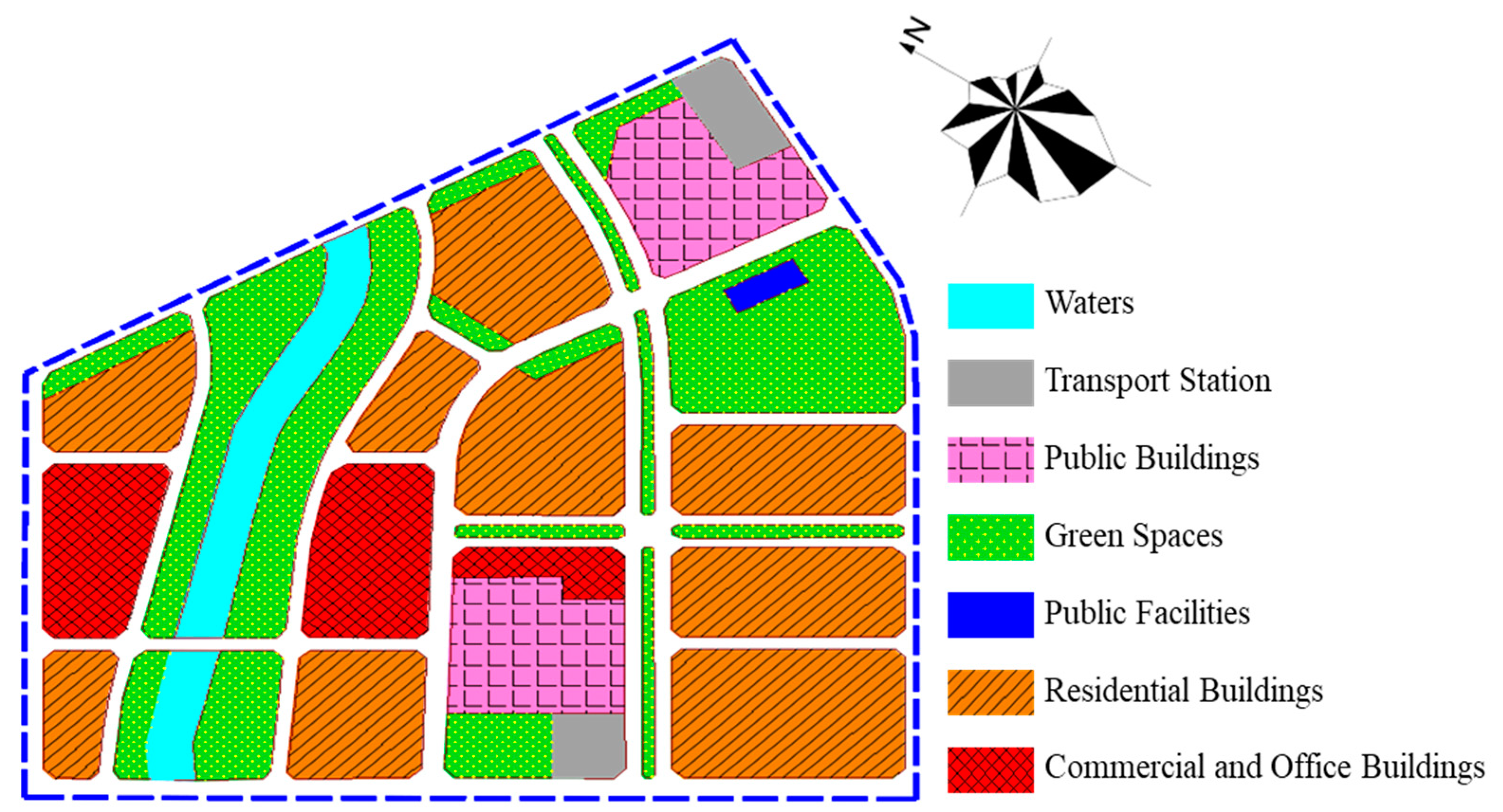
4.1. Case Description

This section presents a case study from a major multi-heat source heating district in Harbin, covering an area of 1,264,800 m² and comprising residential, public, commercial, and office buildings.

Table 1. Building user-related information.

Type of Building	$\mathbf{Area}\left({10}^4{\mathbf{m}}^2\right)$	Design Heating Index $\left(\mathbf{W}/{\mathbf{m}}^2\right)$	$\mathbf{Design}\mathbf{Heat}\mathbf{Load}\left(\mathbf{MW}\right)$
Residential	66.36	40	26.54
Public	22.80	65	14.82
Commercial	20.24	60	12.14
Office	17.08	60	10.24

provides details on the areas and designed heat loads for each type of heat-consuming building.

Figure 5 depicts the schematic plan of the studied district. The heating season extends over 176 days, during which the district records an average outdoor temperature of −9.4 °C and an extreme low of −24.2 °C. The employed heating strategy features a multi-energy complementary system, building upon conventional designs. The system’s designed supply and return temperatures are set at 50/40 °C.

Table 2. Regional heat source information.

Type of Source	$\mathbf{Proportion}\left(\%\right)$	$\mathbf{Design}\mathbf{Heat}\mathbf{Capacity}\left(\mathbf{MW}\right)$
Gas turbine (GT)	37.28	23.78
Coal fired boiler (CFB)	32.14	20.50
Gas fired boiler (GFB)	10.19	6.50
Ground source heat pump (GSHP)	10.19	6.50
Air source heat pump (ASHP)	10.19	6.50

details the types and load ratios of the utilized heat sources.

The plan is to optimize the heating system, designating residential buildings as interval temperature control users. Public and office buildings are designated as general users; commercial buildings as flexible load users. In the traditional system, the interior temperature for all users was set at 18 °C. Previous studies on building characteristics in this area indicated an average temperature difference of 9.8 °C between neighboring residential units. Therefore, in this case study, the redesigned system’s interval temperature control is set to [18,28]. The value of (${\omega }_{\min }$) is set at 80%, which is an estimate derived from the case calculations presented in this paper. Following optimized, the temperature distribution among interval temperature control users still aligns symmetrically around the mean, supporting the hypothesis.

4.2. Operation Scheduling Model of Case

4.2.1. Objective Function

Following optimization, the district heating system operates with three primary objectives. These objectives include: reducing carbon emissions, enhancing economic efficiency, and achieving an integrated target that balances both carbon emissions and economic considerations. The objective functions for each goal are defined as follows:

(1) Carbon emission:

$$Min{f}_{Carbon}=Min\left({\displaystyle \sum _{t=0}^{period}{\displaystyle \sum _{i=1}^n\frac{Q_{source\_i}\left(t\right)}{{\eta }_i\left(t\right)}\cdot c{e}_i}}\right)$$

(43)

(2) Economic efficiency:

$$Min{g}_{Economy}=Min\left({\displaystyle \sum _{t=0}^{period}{\displaystyle \sum _{i=1}^n\frac{Q_{source\_i}\left(t\right)}{{\eta }_i\left(t\right)}\cdot c{c}_i}}\right)$$

(44)

(3) Integrated targe:

$$Min{f}_1=Min\left(\alpha f_{Carbon}^{\prime }+\beta g_{Economy}^{\prime }\right)$$

(45)

The calculation methods for $f_{Carbon}^{\prime }$ and $g_{Economy}^{\prime }$ are presented in Equations (29) and (30), respectively. The lower-level objective function of the system is defined as a user-adjustable temperature range function, as demonstrated in Equation (34).

4.2.2. Heat Source Model and Other Parameters

Different Heat source vary not only in their operational efficiency and fuel usage but also in the methods used to calculate their carbon emissions and economic viability. The calculation models applied to the heating sources discussed in this case study are outlined as follows:

(1) GT. When the capacity of these gas turbines ranges from 1.15 kW to 45.00 MW, the calculation model for the equipment is as follows [34]:

$$F_{gt}\left(t\right)={\displaystyle \frac{E_{gt}\left(t\right)}{{\eta }_{gt}\left(t\right)}}$$

(46)

$$E_{gt}\left(t\right)={\displaystyle \frac{Q_{\mathrm{gt}}\left(t\right)}{{{\alpha }^{\prime }}_{gt}}}$$

(47)

$${\alpha }_{gt}^{\prime }={\displaystyle \frac{0.7536-{\left({\mathrm{C}}_{gt}\right)}^2\times {10}^{-10}+8\times {10}^{-10}\left({\mathrm{C}}_{gt}\right)}{-{\left({\mathrm{C}}_{gt}\right)}^2\times {10}^{-10}+8\times {10}^{-10}\left({\mathrm{C}}_{gt}\right)+0.2464}}$$

(48)

$${\eta }_{gt}\left(t\right)=\left[-1.18PL{R}_{gt}{\left(t\right)}^4+3.69PL{R}_{gt}{\left(t\right)}^3-4.69PL{R}_{gt}{\left(t\right)}^2+3.18PL{R}_{gt}\left(t\right)\right]{\eta }_{gt}^{nom}$$

(49)

$$PL{R}_{gt}\left(t\right)={\displaystyle \frac{E_{gt}\left(t\right)}{C_{gt}}}$$

(50)

$${\eta }_{gt}^{nom}=-{\left({\mathrm{C}}_{gt}\right)}^2\times {10}^{-10}+8\times {10}^{-10}\left({\mathrm{C}}_{gt}\right)+0.2464$$

(51)

where $F_{gt}\left(t\right)$ represents the fuel consumption of gas turbine at time t (MWh); $E_{gt}\left(t\right)$ refers the gas turbine power generation at time t (MW); ${\eta }_{gt}\left(t\right)$ signifies the nominal power generation efficiency of the gas turbine (%); $Q_{\mathrm{gt}}\left(t\right)$ indicates the heat load of gas turbine at time t (MW); $PL{R}_{gt}\left(t\right)$ signifies the partial load rate of the gas turbine at time t, $PL{R}_{gt}\subset \left[0.2,1.0\right]$; ${\mathrm{C}}_{gt}$ denotes the rated power generation of the gas turbine (MW), $\left({\mathrm{C}}_{gt}\subset \left[1.15,45.00\right]\right)$; ${\eta }_{gt}^{nom}$ represents the nominal power generation efficiency of the gas turbine (%); ${{\alpha }^{\prime }}_{gt}$ signifies the nominal power generation efficiency of the gas turbine (%).

(2) CFB.

$$F_{cfb}\left(t\right)={\displaystyle \frac{Q_{cfb}\left(t\right)}{{\eta }_{cfb}\left(t\right)}}$$

(52)

$${\eta }_{cfb}\left(t\right)={\eta }_{cfb}^{nom}\left(0.0951+1.525PL{R}_{cfb}\left(t\right)-0.6249PL{R}_{cfb}{\left(t\right)}^2\right)$$

(53)

$$PL{R}_{cfb}\left(t\right)={\displaystyle \frac{Q_{\mathrm{cfb}}\left(t\right)}{{Q^{\prime }}_{\mathrm{cfb}}}}$$

(54)

where $F_{cbf}\left(t\right)$ denotes the rated heating capacity of coal-fired boilers (kW); ${\eta }_{cfb}\left(t\right)$ represents the rated thermal efficiency of coal-fired boilers (%); $Q_{cfb}\left(t\right)$ indicates the heat load of coal-fired boilers at time t (MW); $PL{R}_{cfb}\left(t\right)$ signifies the partial load rate of the coal-fired boilers at time t.

(3) GFB:

$$F_{gfb}\left(t\right)={\displaystyle \frac{Q_{gfb}\left(t\right)}{{\eta }_{gfb}}}$$

(55)

where $F_{gfb}\left(t\right)$ represents the rated heating capacity of gas fired boilers (kW); ${\eta }_{gfb}$ denotes the rated thermal efficiency of gas fired boilers (%); $Q_{gfb}\left(t\right)$ indicates the heat load of gas fired boilers at time t (MW); $PL{R}_{cfb}\left(t\right)$ denotes the partial load rate of the coal-fired boilers at time t.

(4) GSHP [35]:

$$E_{gshp}^h\left(t\right)={\displaystyle \frac{Q_{gshp}\left(t\right)}{CO{P}_{\mathrm{gshp}}^h}}$$

(56)

where $E_{gshp}^h\left(i\right)$ refers the power consumption of ground source heat pump at time t (kWh); $Q_{gshp}\left(t\right)$ indicates the heat load of ground source heat pump at time t (MW); $CO{P}_{gshp}^h$ signifies the energy efficiency ratio of ground source heat pump, $CO{P}_{gshp}^h=4.00$.

(5) ASHP [21]:

$$E_{ahp}^h\left(t\right)={\displaystyle \frac{Q_{ahp}\left(t\right)}{CO{P}_{\mathrm{ahp}}^h\left(t\right)}}$$

(57)

$$CO{P}_{\mathrm{ahp}}^h\left(t\right)=CO{P^{\prime }}_{\mathrm{ahp}}^h{\left({\displaystyle \frac{{\mathrm{T}}_w\left(t\right)+273.15}{{\mathrm{T}}_{ahp\_out}+273.15}}\right)}^{5.89}$$

(58)

where $E_{ahp}^h\left(t\right)$ denotes the power consumption of air source heat pump at time t (kWh); $Q_{ahp}\left(t\right)$ indicates the heat load of air source heat pump at time t (MW); $CO{P}_{ahp}^h$ signifies the energy efficiency ratio of air source heat pump, $CO{P^{\prime }}_{ahp}^h=2.46$; ${\mathrm{T}}_{ahp\_out}$ represents air source heat pump design outdoor temperature under heating conditions, ${\mathrm{T}}_{ahp\_out}^{\text{′}}=-12°\mathrm{C}$.

The heat load of the heating system is calculated using the following methods:

$$Q_{GU}\left(t\right)={\displaystyle \frac{T_{in\_GU}^{\prime }-T_{out}\left(t\right)}{T_{in\_GU}^{\prime }-T_{out}^{\prime }}}\cdot {\kappa }_{GU}\cdot A_{GU}$$

(59)

$$Q_{FLU}\left(t\right)={\displaystyle \frac{T_{in\_FLU}^{\prime }-T_{out}\left(t\right)}{T_{in\_FLU}^{\prime }-T_{out}^{\prime }}}\cdot {\kappa }_{FLU}\cdot A_{FLU}$$

(60)

$$Q_{DSU}\left(t\right)={\displaystyle \frac{\overline{T_{in}}-T_{out}\left(t\right)}{T_{in\_DSU}^{\prime }-T_{out}^{\prime }}}\cdot {\kappa }_{DSU}\cdot A_{DSU}$$

(61)

where $Q_{GU}\left(t\right)$ denotes the heat load of general users at time t (MW); $Q_{FLU}\left(t\right)$ represents the heat load of flexible load users at time t (MW); $Q_{DSU}\left(t\right)$ indicates the heat load of interval temperature control users at time t (MW); $T_{in\_GU}^{\prime },T_{in\_FLU}^{\prime },T_{in\_DSU}^{\prime }$ represents the designed indoor temperature for general users, flexible load users, interval temperature control users (°C); ${\kappa }_{GU},{\kappa }_{FLU},{\kappa }_{DSU}$ refers the designed heating index for general users, flexible load users, interval temperature control users $\left(\mathrm{W}/{\mathrm{m}}^2\right)$; $A_{GU},A_{FLU},A_{DSU}$ signifies the total building area for general users, flexible load users, interval temperature control users $\left({\mathrm{m}}^2\right)$.

In district heating systems, the thermal capacity of buildings, where the rate of temperature change in their thermal storage does not exceed 0.1 °C/h, can be calculated as follows [36]:

$$C_{building}=1.1641A_{building}+1030.9$$

(62)

where $C_{building}$ indicates the standard heat capacity of building $\left(\mathrm{MJ}/°\mathrm{C}\right)$; $A_{building}$ denotes the building area $\left({\mathrm{m}}^2\right)$.

Other relevant parameters in the calculation process are shown in the following table (

Table 3. Other relevant calculation parameters.

Economic Parameter	Value	Carbon Emission Parameters	Value
Gas unit price	$3.5\yen /{\mathrm{m}}^3$	Gas carbon emission coefficient	$55.612t/\mathrm{TJ}$
Gas calorific value	$389.31\mathrm{GJ}/10^4{\mathrm{m}}^3$	Coal carbon emission coefficient	$101.448t/\mathrm{T}\mathrm{J}$
Coal unit price	$840\yen /t$	Power carbon emission coefficient	$1.036\mathrm{t}\mathrm{C}{\mathrm{O}}_2/\mathrm{M}\mathrm{W}\cdot \mathrm{h}$
Coal caloric value	$29.27\mathrm{GJ}/t$	$\alpha$	0.5
Electricity unit price	$0.7165\yen /\mathrm{kW}\cdot \mathrm{h}$	$\beta$	0.5

):

4.3. Result and Discussed

4.3.1. Case Description

In the case study, the increment of the system’s heat load, following the optimization of the traditional multi-source heating system, is calculated using Equation (8) to be 3173 kW, accounting for 4.98% of the total design heat load. The duration of the adjustable temperature range, calculated using Equation (17), is 3494 h (approximately 145.6 days), representing 82.7% of the total heating season. As a result, expanding the heat source capacity is unnecessary. The annual total heat supply of the traditional heating system under design conditions is calculated using Equation (23) to be 645.3 TJ. Following optimization, it increases to 691.8 TJ, reflecting a 7.22% growth. The critical outdoor temperature for the optimized system, calculated using Equation (10), is −22.1 °C.

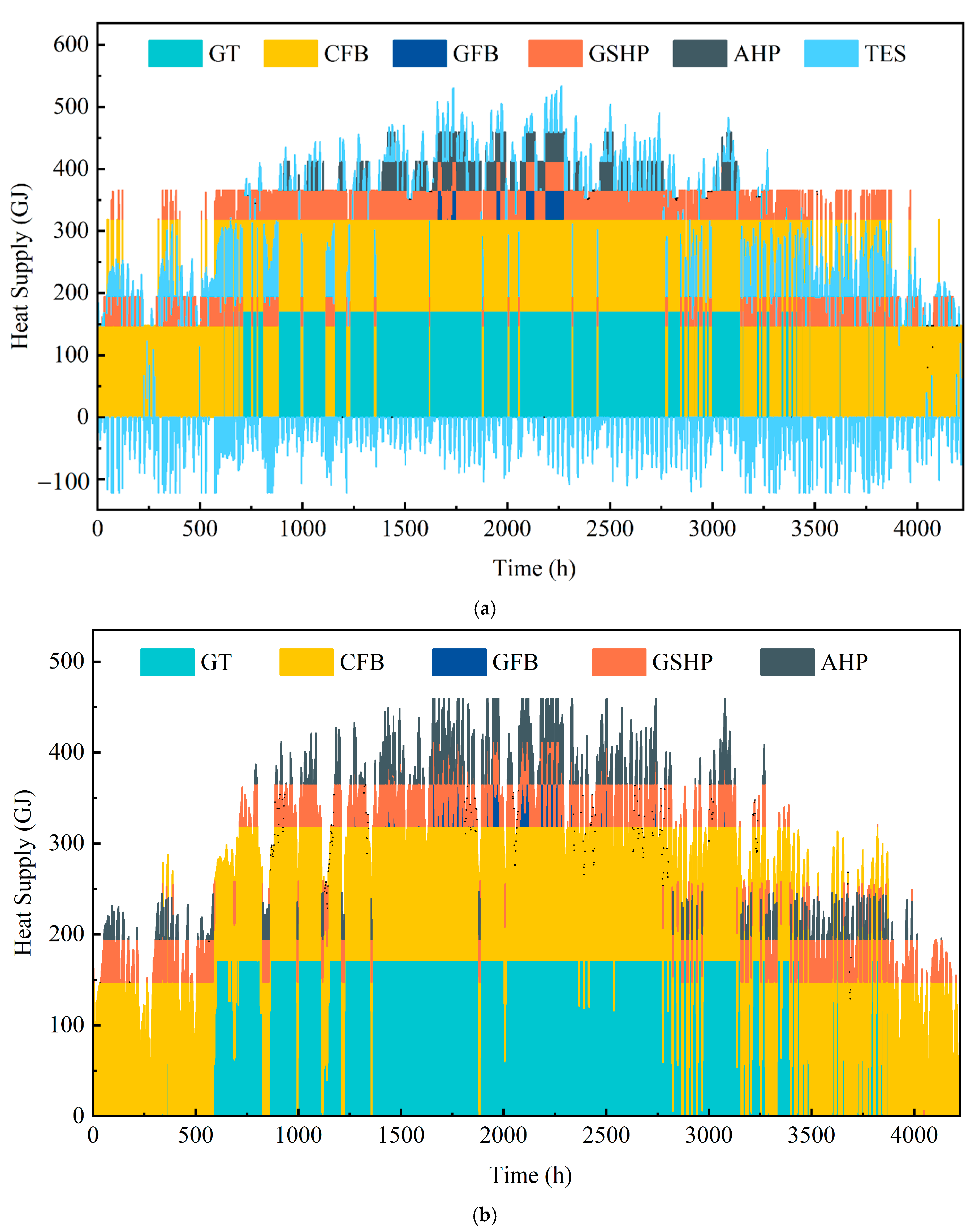
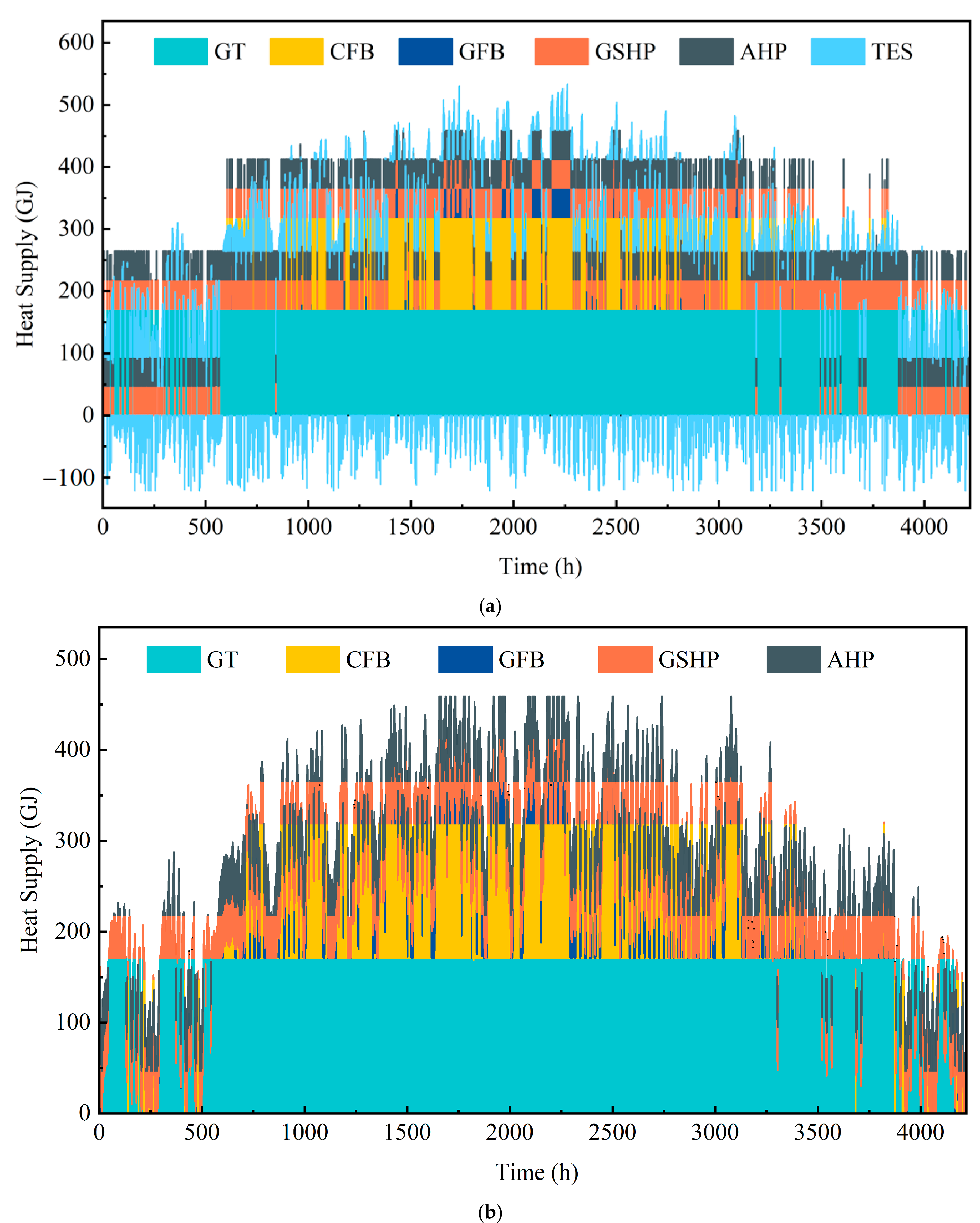
4.3.2. Operation Optimization

Based on a typical heating season in Harbin, which features hourly adjustments and daily heat storage and release cycles, this study optimizes the operational regulation of the system throughout the heating season. The system operation objectives are categorized into three types: economically optimal, carbon emission-reducing, and comprehensively optimal. This paper employs the Python programming language and the advanced solver package ‘CPLEX 22.1.0’ to address the operational scheduling models of the heating system, both before and after optimization.

In practice, the durations of the different adjustable temperature intervals of the optimized heating system are detailed in

Table 4. The optimized heating system’s temperature intervals and duration.

Adjustable Temperature Intervals (°C)	Temperature Interval Size (°C)	Continuous Days (day)	Percentage (%)
[18,28] (Design adjustable temperature range)	10	169	96.02
[18,27]	9	1	0.57
[18,22]	4	2	1.14
[18,20]	2	2	1.14
18	0	2	1.14

below.

Table 4 shows that during the heating season, without expanding heat sources in the optimized system, the designed adjustable temperature ranges persisted for 169 days, representing 96.02% of the season. In contrast, the number of days with temperature ranges below 5 °C was limited to just six, constituting 3.42% of the season. These results confirm that the system effectively met user thermal demands within the specified temperature intervals, even without enhanced heat source capacity. The actual operational dispatch saw a 16.55% increase in the duration of the adjustable temperature ranges compared to the designed conditions.

The primary reason for this outcome was the use of days as units for adjusting temperature ranges in the control of the optimized system during actual operation. In this scenario, the system fully utilized commercial buildings as flexible load users, leveraging their thermal storage and release capacities to shift loads and supplement heat when outdoor temperatures fell below the critical threshold, thus sustaining heating capacity throughout the operational day. Furthermore, this outcome implies that during the optimization of traditional heating systems, setting the sustainable duration of adjustable temperature ranges too long may lead to unnecessary heat source expansions.

Figure 6, Figure 7 and Figure 8 present the results obtained through the optimized dispatch model, showcasing the system’s economic, carbon emission, and comprehensive optimization before and after the modifications, respectively. These results are derived from calculations that specifically aimed at achieving optimal economic operations, minimizing carbon emissions, and obtaining the best comprehensive performance.

These figures demonstrate that the heat loads borne by different heat sources vary significantly during the operation of the heating system under different operational objectives. When the system’s operational objective prioritizes economic efficiency, the largest heat load is assumed by the coal-fired boiler. Conversely, when the operational objectives aim at reducing carbon emissions and incorporating comprehensive considerations, the gas turbine bears the maximum heat load. Compared to traditional heating systems, the optimized heating system, impacted by flexible load users, exhibits a more pronounced pattern in the distribution of heat supply from various sources. Furthermore, the duration of full capacity operation of the system’s heat generating equipment is prolonged.

Typically, heat source equipment achieves its highest heating efficiency when operating at rated power. Therefore, the evaluation of heat source equipment efficiency across various systems with differing operational objectives may be conducted by comparing the time fraction that the equipment operates at full load. The time fraction during which the heat source equipment operates at full load is defined by the following equation:

$${\eta }_{S_i}={\displaystyle \frac{{\displaystyle \sum t_{S_i}^e}}{{\displaystyle \sum t_{S_i}}}}\times 100\%$$

(63)

where ${\eta }_{S_i}$ represents the full-load duration ratio of heat source device S_i (%). $t_{S_i}^e$ denotes the duration during which heat source device S_i operates at its rated state, (h). $t_{S_i}$ stands for the total operating time of heat source device S_i during the heating season (h).

The term “full-load duration ratio” refers to the proportion of time that each heat source device operates at full capacity relative to its total operating time during the system’s operation. The specific full-load duration ratios of these devices under various operational objectives for each system are detailed in

Table 5. Full load ratio of heat sources for different operating target conditions of each system.

	Traditional Heating System (%)			Optimized Heating System (%)
	Carbon Emissions	Economic	Integrated	Carbon Emissions	Economic	Integrated
GT	67.52	86.23	90.68	98.92	100.00	100.00
CFB	26.53	74.89	67.17	92.17	99.62	100.00
GFB	58.38	31.05	21.63	85.42	91.43	68.33
GSHP	99.38	62.40	78.03	100.00	85.70	100.00
ASHP	97.86	32.31	62.03	100.00	91.09	86.52

.

The data indicates that, regardless of the operational objective, traditional heating systems consistently demonstrate a lower full-load duration ratio of heat source devices compared to those in optimized systems, although variations exist among different heat sources. As shown in Figure 9, the comparison of full-load duration ratio increments between traditional and optimized heating systems under various operational objectives reveals notable differences. Specifically, coal-fired boilers, gas boilers, and air-source heat pumps show relatively large increments in both system types. The highest increment for coal-fired boilers, reaching 65.64%, occurs under carbon emission objectives. For gas boilers and air-source heat pumps, the greatest increments, 60.38% and 58.78% respectively, are observed under economic objectives. Conversely, gas turbines and ground-source heat pumps show smaller increases in full-load duration ratios, with maximum values of 31.4% and 23.3% under carbon emission and economic objectives, respectively.

In the context of China’s district heating systems, which are predominantly centralized and seldom account for the individualized thermal load demands of residential buildings, no established standards currently exist for interval temperature control capabilities at the user level. Prior to optimization, traditional heating systems theoretically achieve a maximum design temperature interval coverage duration of only 82.7%, which is 13.32% lower than the 96.02% achieved by the optimized systems presented in this study. Regarding heat source efficiency, traditional heating systems exhibit a full-load duration ratio of 63.73%, whereas the optimized systems achieve a full-load duration ratio of 93.28%, representing an improvement of 29.54%. These enhancements demonstrate the significant potential of demand-side-oriented modifications in improving both operational efficiency and the ability to meet variable thermal demands within district heating systems.

When carbon emissions are the operational objective, there is a noticeable improvement in the efficiency of traditional heat sources (GT, CFB) within optimized heating systems, with an average increase of 48.52% in the full-load duration ratio of devices. Conversely, when economic viability is the operational objective, there is a marked improvement in the efficiency of clean energy heat sources (GFB, GSHP, ASHP), with an average increase of 47.49% in the full-load duration ratio of devices.

These outcomes can be attributed to two key factors in the optimized heating system. First, the inclusion of users with autonomously regulated temperature demands has led to an increase in the average heat load of the heat sources, which has subsequently enhanced the full-load duration ratio of each heating device. Second, the optimized system employs flexible-load users to balance and shift peak and valley loads, significantly reducing fluctuations in the heat load across the heat sources. This stabilization decreases the frequency of on-off cycling of the heat sources, thereby extending the full-load operating time of the heating devices.

When evaluated under operational conditions during a typical heating season, the total heat output of the conventional heating system was calculated to be 615.54 TJ. Following an optimization retrofit, the total heat output under identical conditions increased to 663.76 TJ, representing a 7.83% increase in heat output compared to the conventional system. This exceeds the 7.22% growth rate when control is based on an hourly unit. These findings are consistent with the inferences drawn earlier in the text.

Based on the operational objectives of the traditional heating system in the case study,

Table 6. Relative growth rates of annual operating costs and carbon emissions under each operating target.

	Carbon Emissions	Economic	Integrated
Relative growth rates of annual operating costs (%)	4.07	6.14	7.79
Relative growth rates of annual carbon emissions (%)	5.72	2.45	1.27

shows the relative growth rates of annual operating costs and carbon emissions for the constructed flexible intelligent heating system under each operational objective. The relative growth rates calculate the increases in annual operating costs and carbon emissions under the same operational objectives for both types of heating systems. The table indicates that when both operating costs and carbon emissions are considered as operational objectives, annual operating costs increase by 7.79%, while annual carbon emissions increase by only 1.27%. Furthermore, regardless of the operational objective adopted by the system, the increases in annual operating costs and carbon emissions for the constructed flexible intelligent heating system are less than the increase in the required heating supply. This also confirms, from another perspective, that the overall efficiency of the system improves when the traditional heating system is upgraded to a flexible intelligent heating system.

5. Conclusions

This paper investigates the optimization and transformation methods of demand-side-oriented traditional heating systems. In terms of design, the basic process of system optimization and transformation is elucidated, and key design parameters are proposed to achieve a shift from source-end dominance to demand-end dominance. In terms of operation, a dual-layer planning model for system operation scheduling is established to address both the adjustable temperature range for users and the performance indicators of the heat source system during regulation. The main conclusions are as follows:

• Without expanding the heat source capacity of the traditional heating system, the optimized system can still provide residential users with long-term interval control capabilities. In the case study system, the designed adjustable temperature range for residential buildings accounts for 96.02% of the entire heating season, with the duration of the adjustable temperature range falling below half for only 6 days.
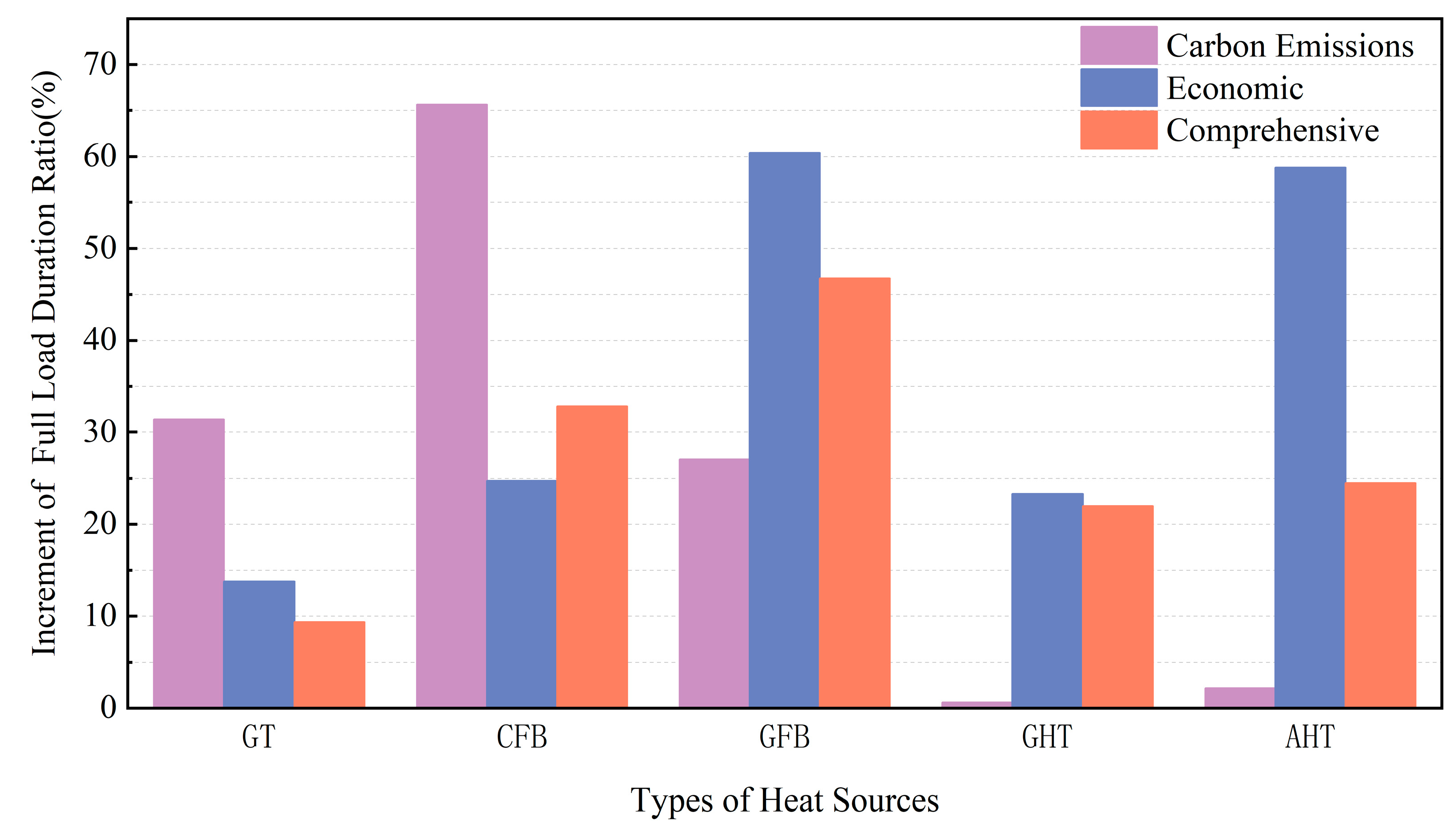
• The overall efficiency of the optimized system will be enhanced, with the heat source equipment operating at full load for longer durations. In the case study system, the average full load duration ratio of the heat source equipment in the transformed system increased by 29.54%.
• After optimization and renovation, the increase in user comfort requirements led to an enhancement of the overall heating capacity of the system. However, regardless of the operating target the system adopts, the growth rate of annual operating costs and carbon emissions is lower than that of the annual heating capacity.

In future studies, we will further explore the optimal values for the heating season duration ratio that meets the design requirements for adjustable temperature ranges, aiming to accommodate a wider variety of heating climates. Additionally, we will investigate the impact of varying the weight factors α and β, which represent carbon emissions and economic considerations, respectively, within the bi-level optimization model. This will be conducted under different heating climate regions and diverse heat source equipment conditions to understand their effects on the system’s comprehensive optimization objectives. These advancements will provide deeper insights and more tailored solutions for the optimization and transformation of heating systems across diverse environmental and operational contexts.

References

1. Buffa, S.; Cozzini, M.; D’antoni, M.; Baratieri, M.; Fedrizzi, R. 5th generation district heating and cooling systems: A review of existing cases in Europe. Renew. Sustain. Energy Rev. 2019, 104, 504–522. [Google Scholar] [CrossRef]
2. Prina, M.G.; Manzolini, G.; Moser, D.; Nastasi, B.; Sparber, W. Classification and challenges of bottom-up energy system models—A review. Renew. Sustain. Energy Rev. 2020, 129, 109917. [Google Scholar] [CrossRef]
3. Edtmayer, H.; Nageler, P.; Heimrath, R.; Mach, T.; Hochenauer, C. Investigation on sector coupling potentials of a 5th generation district heating and cooling network. Energy 2021, 230, 120836. [Google Scholar] [CrossRef]
4. Lund, H.; Østergaard, P.A.; Chang, M.; Werner, S.; Svendsen, S.; Sorknæs, P.; Thorsen, J.E.; Hvelplund, F.; Mortensen, B.O.G.; Mathiesen, B.V.; et al. The status of 4th generation district heating: Research and results. Energy 2018, 164, 147–159. [Google Scholar] [CrossRef]
5. Lauenburg, P.; Wollerstrand, J. Adaptive control of radiator systems for a lowest possible district heating return temperature. Energy Build. 2014, 72, 132–140. [Google Scholar] [CrossRef]
6. Sun, C.; Chen, J.; Cao, S.; Gao, X.; Xia, G.; Qi, C.; Wu, X. A dynamic control strategy of district heating substations based on online prediction and indoor temperature feedback. Energy 2021, 235, 121228. [Google Scholar] [CrossRef]
7. Saletti, C.; Zimmerman, N.; Morini, M.; Kyprianidis, K.; Gambarotta, A. Enabling smart control by optimally managing the State of Charge of district heating networks. Appl. Energy 2021, 283, 116286. [Google Scholar] [CrossRef]
8. Gustafsson, J.; Delsing, J.; van Deventer, J. Improved district heating substation efficiency with a new control strategy. Appl. Energy 2010, 87, 1996–2004. [Google Scholar] [CrossRef]
9. Ma, Z.; Knotzer, A.; Billanes, J.D.; Jørgensen, B.N. A literature review of energy flexibility in district heating with a survey of the stakeholders’ participation. Renew. Sustain. Energy Rev. 2020, 123, 109750. [Google Scholar] [CrossRef]
10. Coss, S.; Verda, V.; Le-Corre, O. Multi-objective optimization of district heating network model and assessment of demand side measures using the load deviation index. J. Clean. Prod. 2018, 182, 338–351. [Google Scholar] [CrossRef]
11. Saletti, C.; Zimmerman, N.; Morini, M.; Kyprianidis, K.; Gambarotta, A. A control-oriented scalable model for demand side management in district heating aggregated communities. Appl. Therm. Eng. 2022, 201, 117681. [Google Scholar] [CrossRef]
12. Yin, R.; Kara, E.C.; Li, Y.; DeForest, N.; Wang, K.; Yong, T.; Stadler, M. Quantifying flexibility of commercial and residential loads for demand response using setpoint changes. Appl. Energy 2016, 177, 149–164. [Google Scholar] [CrossRef]
13. Hedegaard, R.E.; Kristensen, M.H.; Pedersen, T.H.; Brun, A.; Petersen, S. Bottom-up modelling methodology for urban-scale analysis of residential space heating demand response. Appl. Energy 2019, 242, 181–204. [Google Scholar] [CrossRef]
14. Guelpa, E.; Marincioni, L. Demand side management in district heating systems by innovative control. Energy 2019, 188, 116037. [Google Scholar] [CrossRef]
15. Zhong, J.J.; Li, Y.; Wu, Y.; Cao, Y.J.; Li, Z.M.; Peng, Y.J.; Qiao, X.B.; Xu, Y.; Yu, Q.; Yang, X.S.; et al. Optimal Operation of Energy Hub: An Integrated Model Combined Distributionally Robust Optimization Method With Stackelberg Game. IEEE Trans. Sustain. Energy 2023, 14, 1835–1848. [Google Scholar] [CrossRef]
16. Zou, Y.Y.; Xu, Y.; Li, J.Y. Aggregator-Network Coordinated Peer-to-Peer Multi-Energy Trading via Adaptive Robust Stochastic Optimization. IEEE Trans. Power Syst. 2024, 39, 7124–7137. [Google Scholar] [CrossRef]
17. Department of Energy’s Office of Energy Efficiency and Renewable Energy. Geothermal Electricity Technology Evaluation Model (GETEM); Department of Energy’s Office of Energy Efficiency and Renewable Energy: Washington, DC, USA, 2020. [Google Scholar]
18. Goy, S.; Ashouri, A.; Maréchal, F.; Finn, D. Estimating the potential for thermal load management in buildings at a large scale: Overcoming challenges towards a replicable methodology. Energy Procedia 2017, 111, 740–749. [Google Scholar] [CrossRef]
19. Lund, R.; Mathiesen, B.V. Large combined heat and power plants in sustainable energy systems. Appl. Energy 2015, 142, 389–395. [Google Scholar] [CrossRef]
20. Rong, A.; Figueira, J.R.; Lahdelma, R. A two phase approach for the bi-objective non-convex combined heat and power production planning problem. Eur. J. Oper. Res. 2015, 245, 296–308. [Google Scholar] [CrossRef]
21. Wei, W.; Ni, L.; Zhou, C.; Yao, Y.; Xu, L.; Yang, Y. Performance analysis of a quasi-two stage compression air source heat pump in severe cold region with a new control strategy. Appl. Therm. Eng. 2020, 174, 115317. [Google Scholar] [CrossRef]
22. Benalcazar, P. Optimal sizing of thermal energy storage systems for CHP plants considering specific investment costs: A case study. Energy 2021, 234, 121323. [Google Scholar] [CrossRef]
23. Jin, T. The effectiveness of combined heat and power (CHP) plant for carbon mitigation: Evidence from 47 countries using CHP plants. Sustain. Energy Technol. Assess. 2022, 50, 101809. [Google Scholar] [CrossRef]
24. Li, Y.; Fu, L.; Zhang, S.; Zhao, X. A new type of district heating system based on distributed absorption heat pumps. Energy 2011, 36, 4570–4576. [Google Scholar] [CrossRef]
25. Marx, R.; Bauer, D.; Drueck, H. Energy efficient integration of heat pumps into solar district heating systems with seasonal thermal energy storage. Energy Procedia 2014, 57, 2706–2715. [Google Scholar] [CrossRef]
26. Zvingilaite, E.; Balyk, O. Heat savings in buildings in a 100% renewable heat and power system in Denmark with different shares of district heating. Energy Build. 2014, 82, 173–186. [Google Scholar] [CrossRef]
27. Carpaneto, E.; Lazzeroni, P.; Repetto, M. Optimal integration of solar energy in a district heating network. Renew. Energy 2015, 75, 714–721. [Google Scholar] [CrossRef]
28. Kensby, J.; Trüschel, A.; Dalenbäck, J. Heat source shifting in buildings supplied by district heating and exhaust air heat pump. Energy Procedia 2017, 116, 470–480. [Google Scholar] [CrossRef]
29. Turski, M.; Sekret, R. Buildings and a district heating network as thermal energy storages in the district heating system. Energy Build. 2018, 179, 49–56. [Google Scholar] [CrossRef]
30. Li, H.; Wang, Z.; Hong, T.; Piette, M.A. Energy flexibility of residential buildings: A systematic review of characterization and quantification methods and applications. Adv. Appl. Energy 2021, 3, 100054. [Google Scholar] [CrossRef]
31. Dominković, D.; Gianniou, P.; Münster, M.; Heller, A.; Rode, C. Utilizing thermal building mass for storage in district heating systems: Combined building level simulations and system level optimization. Energy 2018, 153, 949–966. [Google Scholar] [CrossRef]
32. Romanchenko, D.; Kensby, J.; Odenberger, M.; Johnsson, F. Thermal energy storage in district heating: Centralised storage vs. storage in thermal inertia of buildings. Energy Convers. Manag. 2018, 162, 26–38. [Google Scholar] [CrossRef]
33. Foteinaki, K.; Li, R.; Heller, A.; Rode, C. Heating system energy flexibility of low-energy residential buildings. Energy Build. 2018, 180, 95–108. [Google Scholar] [CrossRef]
34. Feng, L.; Dai, X.; Mo, J.; Shi, L. Comparison of capacity design modes and operation strategies and calculation of thermodynamic boundaries of energy-saving for CCHP systems in different energy supply scenarios. Energy Convers. Manag. 2019, 188, 296–309. [Google Scholar] [CrossRef]
35. Ren, F.; Wei, Z.; Zhai, X. Multi-objective optimization and evaluation of hybrid CCHP systems for different building types. Energy 2021, 215, 119096. [Google Scholar] [CrossRef]
36. Ding, Y.; Lyu, Y.; Lu, S.; Wang, R. Load shifting potential assessment of building thermal storage performance for building design. Energy 2022, 243, 123036. [Google Scholar] [CrossRef]
Figure 1. The basic structure of a typical heating system.
Buildings 15 00365 g001
Figure 2. The improvement process of the traditional heating system.
Buildings 15 00365 g002
Figure 3. Different types of interval temperature distribution users.
Buildings 15 00365 g003
Figure 4. Mixed integer two-level planning model framework.
Buildings 15 00365 g004
Figure 5. Case area schematic plan.
Buildings 15 00365 g005
Figure 6. (a) The optimal economic solution for the operation of the optimized heating system. (b) The optimal economic solution for the operation of the tradition heating system.
Buildings 15 00365 g006
Figure 7. (a) The optimal carbon emissions solution for the operation of the optimized heating system. (b) The optimal carbon emissions solution for the operation of the tradition heating system.
Buildings 15 00365 g007
Figure 8. (a) The optimal integrated solution for the operation of the optimized heating system. (b) The optimal integrated solution for the operation of the tradition heating system.
Buildings 15 00365 g008
Figure 9. Load rate increment of each heat source device under different system operating targets.
Buildings 15 00365 g009