An Improved Gaussian Mixture Model-Based Data Normalization Method for Removing Environmental Effects on Damage Detection of Structures

Abstract

In structural health monitoring, effectively eliminating the influence of variable environmental conditions on modal frequencies remains a critical challenge for accurate damage identification. Nonstationary and nonlinear variations in modal frequencies, commonly induced by environmental changes, tend to overshadow the effects caused by structural damage. An improved Gaussian mixture model (GMM) is proposed in this paper to normalize nonlinear and nonstationary frequency data, enabling effective structural damage detection under variable environmental conditions. As the effectiveness of the GMM is highly influenced by the initial parameter values used in the expectation-maximization (EM) algorithm, a subdomain division strategy is first presented to determine the unique initial values of the GMM parameters. Through the application of the EM algorithm, the GMM is constructed simply and efficiently through the determined initial parameters. Next, on the basis of the constructed GMM, the modal frequency data are normalized to extract damage features that remain unaffected by environmental variations. Subsequently, Hotelling’s T2 statistic and its cumulative form are calculated for the damage features and designated as the damage indicators; meanwhile, the corresponding damage thresholds are also calculated according to the kernel density estimation technique. To validate the proposed method, two case studies are conducted: one with a numerical mass-spring system and the other with a real bridge structure. Results show that environmental influences no longer impact the normalized frequency data, and the cumulative statistic demonstrates outstanding accuracy in identifying structural damage.

1. Introduction

Through the implementation of structural health monitoring systems, vibration-based damage detection methodologies are progressing rapidly [1,2]. When conducting numerical analysis of structures, the actual damage to the structure usually corresponds to changes in the structural parameters in the finite element model, such as changes in the stiffness matrix [3,4,5]. Numerous structural dynamic characteristics, especially the modal parameters, have been proposed as sensitive indicators for evaluating structural conditions and detecting damage [6,7,8]. Usually, compared to the natural frequency, modal shapes, as well as modal flexibility and strain modes calculated using modal shapes, are more sensitive to minor damage to the structure [9,10,11]. Compared to other modal parameters, the natural frequency is less affected by the placement of sensors in actual data acquisition and analysis [12,13]. Thus, damage indicators are often understood as specific values that illustrate alterations in modal parameters, which are determined through the analysis of vibration data.

While structural damage affects modal frequencies, environmental factors, particularly temperature variations, also play a crucial role during the life cycle of civil structures. According to Liu et al. [14], a year-long monitoring of a concrete bridge revealed that each 1 °C increase in temperature reduced the first three modal frequencies by around 0.8%, 0.7%, and 0.3%. In a laboratory study, Kim et al. [15] discovered that for a steel beam bridge, each 1 °C rise in temperature caused decreases of about 0.64%, 0.33%, 0.44%, and 0.22% in the first four modal frequencies. Cross et al. [16] investigated the influence of wind speed on modal frequencies for the Tamar Bridge, reporting that at higher wind speeds, modal frequencies declined. These findings highlight that environmental factors can alter modal frequencies, thereby masking damage-related indicators.

A major challenge in vibration-based damage detection is defining indicators that respond to structural damage while remaining unaffected by environmental variations [17,18]. Generally, two approaches are employed to address this issue. When environmental condition data are available, linear or nonlinear input–output models can be developed to quantify and eliminate environmental influences on modal frequencies for damage detection. Alternatively, output-only models, such as principal component analysis (PCA) and cointegration analysis (CA), can be utilized to identify relationships among modal frequencies, thereby isolating environmental effects and enhancing damage detection.

Various methods have been utilized to create input–output models linking environmental conditions with modal frequencies, including autoregressive models with exogenous input [19], polynomial regression [20,21], artificial neural networks [22], and Gaussian process regression [23,24]. However, there are at least two limitations regarding the input–output methods [25]: (1) the unavailability of environmental data, often due to sensor malfunctions, may degrade damage detection accuracy, and (2) selecting or accessing the optimal locations for environmental sensors can be problematic. Thus, developing damage detection methods that do not rely on environmental data is of critical importance.

In recent years, there has been growing interest in output-only methods that address the impact of environmental variations on modal frequencies without relying on environmental data measurements. Frequently used methods in this area include the PCA [26,27,28], the nonlinear PCA [29,30], the robust PCA [31], the CA [32,33,34] and the manifold learning [35,36]. Zang et al. [37] developed a subdomain PCA method, which partitions nonlinearly correlated frequency data into linear subdomains. This method facilitates PCA-based modeling and damage detection, effectively minimizing the influence of environmental changes. Since the linear nature of CA may limit its practical applications, Shi et al. [38], Wang et al. [39] and Huang et al. [40] proposed a regime-switching CA method, a localized CA method and a modified regime-switching CA method, respectively, for damage detection considering nonlinearly correlated frequency data. Moreover, Wah et al. [13] proposed to construct polynomial regression models between different orders of modal frequencies for damage detection without environmental measurements. Huang et al. [41] proposed a damage detection method using kernel canonical correlation analysis, specifically designed to manage nonlinear relationships in frequency data. Many of the described output-only approaches operate as projection-like methods, projecting the frequency data into a linear or nonlinear subspace, where indicators are resistant to environmental changes yet highly responsive to structural damage.

There is another output-only method called the Gaussian mixture model (GMM). Kullaa [42] employed the GMM to segment frequency data into distinct clusters where linear model residuals were generated and applied for damage detection under environmental changes. To build a Gaussian mixture model (GMM), the expectation-maximization (EM) algorithm is often employed with initialization from k-means clustering. However, the EM algorithm is highly dependent on the initial parameter values of the GMM [43], with different initializations producing varying GMMs. This variability can result in inconsistent detection outcomes for identical structural damage, thereby reducing the reliability of the GMM-based damage detection approach. One practical solution is to refine the GMM construction algorithm to improve the effectiveness of the damage detection method. Figueiredo et al. [6] suggested employing a Bayesian method to estimate GMM parameters, which allowed the definition of the Mahalanobis squared distance as a damage indicator resistant to environmental variations. To handle damage detection under environmental variations, Santos et al. [44,45] developed two global EM algorithms. These algorithms, based on particle swarm optimization and genetic algorithms, respectively, optimize the Gaussian components and corresponding parameters of the GMM. Although these methods show potential in adaptively constructing GMMs, improvements are still required to enhance stability and minimize dependency on initial parameter settings [46].

A subdomain division strategy is proposed in this study to determine distinct initial parameters for the GMM. These parameters enable the EM algorithm to create a unique GMM, normalizing frequency data for defining damage indicators responsive to structural damage but robust against environmental variations. The paper begins with a review of the conventional EM algorithm for constructing GMMs, followed by an in-depth explanation of the improved GMM (iGMM) method for damage detection. Subsequently, the performance of the method is evaluated using a numerical mass-spring system and a real bridge structure. Detailed conclusions are provided at the end.

2. Methodology

The central focus of the iGMM approach is to determine the unique initial parameters of GMM for the EM algorithm. After reviewing the traditional GMM approach, a subdomain division strategy is proposed to determine the unique initial parameters for constructing the iGMM, specifically using sliding window and generalized likelihood ratio test methods (GLRT) [47]. Then, frequency data are suggested to be normalized via the constructed iGMM. Next, the iGMM is used to normalize frequency data, and damage indicators are calculated using Hotelling’s T² statistic and its cumulative form. Finally, a detailed description of the implementation process for the proposed damage detection method is provided.

2.1. A Review of GMM

GMM is a widely adopted approach for modeling multimodal probability density functions. Let $\mathit{X}=\left[{\mathit{x}}_1,{\mathit{x}}_2,\cdots ,{\mathit{x}}_n\right]$ represent the dataset with $\mathit{n}$ samples, where each sample $\mathit{x}$ contains $\mathit{m}$ features. These features correspond to the modal frequency orders. In general cases, a combination of several Gaussian distributions $p\left(\mathit{x}\right)$ effectively captures the probability density function of multidimensional data $\mathit{x}$.

$$p\left(\mathit{x}\right)={\displaystyle \sum _{k=1}^K{\omega }_k\mathcal{N}\left(\mathit{x}\left|{\mathit{\mu }}_k,{\mathit{C}}_k\right.\right)}$$

(1)

where $K$ is the quantity of Gaussian distributions that constitute the model; $\mathcal{N}\left(\mathit{x}\left|{\mathit{\mu }}_k,{\mathit{C}}_k\right.\right)$ is the probability density function of the k-th Gaussian component; ${\mathit{\mu }}_k$ is the mean vector of the k-th Gaussian component; ${\mathit{C}}_k$ is the covariance matrix of the k-th Gaussian component; ${\omega }_k$ is the k-th mixture coefficient satisfying the constraint that ${\omega }_k>0$ and ${\displaystyle {\sum }_{k=1}^K{\omega }_k}=1$. The specific expression of $\mathcal{N}\left(\mathit{x}\left|{\mathit{\mu }}_k,{\mathit{C}}_k\right.\right)$ is as follows:

$$\mathcal{N}\left(\mathit{x}\left|{\mathit{\mu }}_k,{\mathit{C}}_k\right.\right)={\displaystyle \frac{1}{{\left(2\pi \right)}^{\frac{m}{2}}{\left|{\mathit{C}}_k\right|}^{\frac{1}{2}}}}\exp \left[-{\displaystyle \frac{1}{2}}{\left(\mathit{x}-{\mathit{\mu }}_k\right)}^{\mathrm{T}}{\mathit{C}}_k^{-1}\left(\mathit{x}-{\mathit{\mu }}_k\right)\right]$$

(2)

Let $\mathit{\Theta }={\left\{{\omega }_k,{\mathit{\mu }}_k,{\mathit{C}}_k\right\}}_{k=1}^K$ represent the parameters of GMM. To estimate $\mathit{\Theta }$, the EM algorithm is frequently utilized, as it iteratively converges toward the maximum likelihood estimate [43,46]. The algorithm alternates between the expectation step (E-step) and the maximization step (M-step). In the E-step, the posterior probabilities are determined using the formula provided below:

$$P_{ik}\left(\left.{\mathit{x}}_i\right|\mathit{\Theta }\right)={\displaystyle \frac{{\omega }_k\mathcal{N}\left({\mathit{x}}_i\left|{\mathit{\mu }}_k,{\mathit{C}}_k\right.\right)}{{\displaystyle {\sum }_{j=1}^K{\omega }_j\mathcal{N}\left({\mathit{x}}_i\left|{\mathit{\mu }}_j,{\mathit{C}}_j\right.\right)}}}$$

(3)

In the M-step, the parameter set $\mathit{\Theta }$ is revised using the posterior probability as follows:

$${\omega }_k={\displaystyle \frac{1}{n}}{\displaystyle \sum _{i=1}^n{P}_{ik}\left(\left.{\mathit{x}}_i\right|\mathit{\Theta }\right)}$$

(4)

$${\mathit{\mu }}_k={\displaystyle \frac{{\displaystyle {\sum }_{i=1}^n\left[P_{ik}\left(\left.{\mathit{x}}_i\right|\mathit{\Theta }\right){\mathit{x}}_i\right]}}{{\displaystyle {\sum }_{i=1}^n\left[P_{ik}\left(\left.{\mathit{x}}_i\right|\mathit{\Theta }\right)\right]}}}$$

(5)

$${\mathit{C}}_k={\displaystyle \frac{{\displaystyle {\sum }_{i=1}^n\left[P_{ik}\left(\left.{\mathit{x}}_i\right|\mathit{\Theta }\right)\left({\mathit{x}}_i-{\mathit{\mu }}_k\right){\left({\mathit{x}}_i-{\mathit{\mu }}_k\right)}^{\mathrm{T}}\right]}}{{\displaystyle {\sum }_{i=1}^n\left[P_{ik}\left(\left.{\mathit{x}}_i\right|\mathit{\Theta }\right)\right]}}}$$

(6)

These two steps are executed in an iterative manner until the log-likelihood function $\mathcal{L}\left(\left.\mathit{X}\right|\mathit{\Theta }\right)$, as expressed in Equation (7), reaches a local maximum value.

$$\mathcal{L}\left(\left.\mathit{X}\right|\mathit{\Theta }\right)=\ln {\displaystyle \prod _{i=1}^{n}p\left({\mathit{x}}_i\right)}={\displaystyle \sum _{i=1}^n\ln \left\{{\displaystyle \sum _{k=1}^K{\omega }_k\mathcal{N}\left(\mathit{x}\left|{\mathit{\mu }}_k,{\mathit{C}}_k\right.\right)}\right\}}$$

(7)

The EM algorithm is commonly employed to estimate the parameters of a GMM with a fixed number of Gaussian components. However, its effectiveness depends heavily on the initial parameter values $\mathit{\Theta }$. For damage feature datasets, variations in these initial values can produce inconsistent GMMs, undermining the robustness of the damage detection method. A standard practice is to use k-means clustering to initialize the EM algorithm [48,49], but k-means itself is influenced by its initialization [46]. Additionally, selecting the appropriate number of Gaussian components is critical: too many components can cause overfitting of the damage feature dataset, while too few components may fail to sufficiently capture its probability distribution. Thus, an adaptive approach is needed to construct the GMM, allowing the number of Gaussian components to adjust to the unknown probability distribution of the dataset.

2.2. The Proposed iGMM

To resolve the parameter initialization challenges, the damage feature dataset can be divided into several subsets or subdomains, each assumed to follow a separate Gaussian distribution. This approach inherently determines the number of Gaussian components, as it matches the number of subsets created. Let ${\mathit{X}}_{Init}=\left[{\mathit{x}}_1,{\mathit{x}}_2,\cdots ,{\mathit{x}}_w\right]$ represent the initial window dataset, with a window size $w$. The mean vector and covariance matrix of the dataset ${\mathit{X}}_{Init}$ are calculated and recorded as ${\mathit{\mu }}_{Init}$ and ${\mathit{C}}_{Init}$, respectively. Based on the Gaussian distribution assumption, the probability density of any sample vector $\mathit{x}$ in dataset ${\mathit{X}}_{Init}$ can be written as:

$$p\left(\mathit{x}\left|\mathit{x}\in {\mathit{X}}_{Init}\right.\right)=\mathcal{N}\left(\mathit{x}\left|{\mathit{\mu }}_{Init},\right.{\mathit{C}}_{Init}\right)$$

(8)

Maintaining a constant window size and sliding the window will yield the current window dataset ${\mathit{X}}_{Curr}=\left[{\mathit{x}}_{11},{\mathit{x}}_{12},\cdots ,{\mathit{x}}_{w+10}\right]$, where the sliding distance is set to 10. Similarly, the mean vector and covariance matrix of the dataset ${\mathit{X}}_{Curr}$ are calculated and recorded as ${\mathit{\mu }}_{Curr}$ and ${\mathit{C}}_{Curr}$, respectively. The probability density of an arbitrary sample vector $\mathit{x}$ in the dataset ${\mathit{X}}_{Curr}$ can be expressed by:

$$p\left(\mathit{x}\left|\mathit{x}\in {\mathit{X}}_{Curr}\right.\right)=\mathcal{N}\left(\mathit{x}\left|{\mathit{\mu }}_{Curr},\right.{\mathit{C}}_{Curr}\right)$$

(9)

In this paper, the subdomain division is accomplished based on the GLRT. The GLRT is applied here to determine whether different datasets follow the same distribution. Here, the null hypothesis ${\mathrm{H}}_0$ assumes no significant difference between the current and initial window datasets, while the alternative hypothesis ${\mathrm{H}}_1$ suggests the presence of such a difference.

$$\left\{\begin{array}{cccc}{\mathrm{H}}_0:& {\mathit{\mu }}_{Curr}={\mathit{\mu }}_{Init}& and& {\mathit{C}}_{Curr}={\mathit{C}}_{Init}\\ {\mathrm{H}}_1:& {\mathit{\mu }}_{Curr}\ne {\mathit{\mu }}_{Init}& or& {\mathit{C}}_{Curr}\ne {\mathit{C}}_{Init}\end{array}\right.$$

(10)

The test statistic is expressed by [37]:

$${\mathrm{T}}_{glr}\left(\mathit{x}\left|\mathit{x}\in {\mathit{X}}_{Curr}\right.\right)={\displaystyle \sum _{i=1}^w\ln \frac{p\left({\mathit{x}}_i\left|{\mathit{x}}_i\in {\mathit{X}}_{Curr};{\mathrm{H}}_1\right.\right)}{p\left({\mathit{x}}_i\left|{\mathit{x}}_i\in {\mathit{X}}_{Curr};{\mathrm{H}}_0\right.\right)}}>\gamma$$

(11)

where $\gamma$ is the critical value, which corresponds to a significance level of 0.05. If Equation (11) holds, the current window dataset and the initial window dataset do not belong to the same subdomain. If Equation (11) does not hold, the current window dataset and the initial window dataset belong to the same subdomain. The aforementioned process is repeated until the entire dataset is divided into different subdomains. When the damage feature dataset is divided into different subsets/subdomains, the initial values of the parameter set $\mathit{\Theta }$ can be determined. Let ${\mathit{X}}_k=\left[{\mathit{x}}_{k,1},{\mathit{x}}_{k,2},\cdots ,{\mathit{x}}_{k,n_k}\right]$ represent the k-th divided subsets/subdomains where $n_k$ is the sample number of ${\mathit{X}}_k$. If the number of divided subsets/subdomains is $K$, the initial parameter value can be calculated by:

$${\omega }_k^{\left(0\right)}={\displaystyle \frac{n_k}{{\displaystyle {\sum }_{k=1}^K{n}_k}}}$$

(12)

$${\mathit{\mu }}_k^{\left(0\right)}={\displaystyle \frac{1}{n_k}}{\displaystyle \sum _{i=1}^{n_k}{\mathit{x}}_{k,i}}$$

(13)

$${\mathit{C}}_k^{\left(0\right)}={\displaystyle \frac{1}{n_k-1}}{\displaystyle \sum _{i=1}^{n_k}\left({\mathit{x}}_{k,i}-{\mathit{\mu }}_k^{\left(0\right)}\right){\left({\mathit{x}}_{k,i}-{\mathit{\mu }}_k^{\left(0\right)}\right)}^{\mathrm{T}}}$$

(14)

where ${\omega }_k^{\left(0\right)}$, ${\mathit{\mu }}_k^{\left(0\right)}$ and ${\mathit{C}}_k^{\left(0\right)}$ are the initial values of ${\omega }_k$, ${\mathit{\mu }}_k$ and ${\mathit{C}}_k$, respectively. After the initialization process for the parameter values is completed, the EM algorithm is applied to obtain the unique GMM (i.e., the iGMM) for the damage feature dataset.

2.3. Data Normalization

When the i-th data vector ${\mathit{x}}_i$ in the damage feature dataset is assumed to be sampled from a Gaussian distribution with a mean vector $\mathit{\mu }$ and a covariance matrix $\mathit{C}$, this data vector can be normalized as follows:

$${\tilde{\mathit{x}}}_i={\sum }^{-1/2}\left({\mathit{x}}_i-\mathit{\mu }\right)$$

(15)

where $\tilde{\mathit{x}}$ is the normalized data vector for $\mathit{x}$, and $\sum$ represents a diagonal matrix where each element matches the respective diagonal entry of the covariance matrix $\mathit{C}$.

However, according to the previous discussion, the data vector ${\mathit{x}}_i$ is sampled from a GMM. This data vector can therefore be normalized as follows:

$${\tilde{\mathit{x}}}_i={\displaystyle \sum _{k=1}^K{P}_{ik}\left(\left.{\mathit{x}}_i\right|\mathit{\Theta }\right)\cdot {\sum }_k^{-1/2}\left({\mathit{x}}_i-{\mathit{\mu }}_k\right)}$$

(16)

where $P_{ik}\left(\left.{\mathit{x}}_i\right|\mathit{\Theta }\right)$ represents the posterior probability of the i-th data vector ${\mathit{x}}_i$ belonging to the k-th Gaussian component within the constructed iGMM, and ${\sum }_k$ represents a diagonal matrix where each element matches the respective diagonal entry of the covariance matrix ${\mathit{C}}_k$.

2.4. Damage Indicator and Threshold

After the data normalization process is completed for the damage feature dataset, the damage indicator can be defined for each normalized data vector. The mean vector and covariance matrix of the normalized dataset are represented by $\tilde{\mathit{\mu }}$ and $\tilde{\mathit{C}}$, respectively. The damage indicator, known as Hotelling’s T² statistic, also referred to as the Mahalanobis squared distance, is defined as:

$${\mathrm{T}}^2\left(i\right)={\left({\tilde{\mathit{x}}}_i-\tilde{\mathit{\mu }}\right)}^{\mathrm{T}}{\tilde{\mathit{C}}}^{-1}\left({\tilde{\mathit{x}}}_i-\tilde{\mathit{\mu }}\right)$$

(17)

where ${\mathrm{T}}^2\left(i\right)$ is Hotelling’s T² statistic for the i-th normalized data vector ${\tilde{\mathit{x}}}_i$.

However, Hotelling’s T² statistic is perhaps insensitive to small structural damages. In this situation, several consecutive data samples can be used together to construct a cumulative statistic. Based on $s$ consecutive samples, the cumulative T² statistic is used as the damage indicator and can be calculated by:

$${\mathrm{T}}_{Cum}^2\left(i\right)={\displaystyle \frac{1}{s}}{\displaystyle \sum _{j=1}^s{\mathrm{T}}^2\left(i-j+1\right)}={\displaystyle \frac{1}{s}}{\displaystyle \sum _{j=1}^s{\left({\tilde{\mathit{x}}}_{i-j+1}-\tilde{\mathit{\mu }}\right)}^{\mathrm{T}}{\tilde{\mathit{C}}}^{-1}\left({\tilde{\mathit{x}}}_{i-j+1}-\tilde{\mathit{\mu }}\right)}$$

(18)

where ${\mathrm{T}}_{Cum}^2\left(i\right)$ is the cumulative T² statistic for the i-th normalized data vector ${\tilde{\mathit{x}}}_i$. It is obvious that the cumulative T² statistic will be Hotelling’s T² statistic when $s=1$.

The damage threshold can be theoretically determined when the normalized data vectors (under the intact state of the monitored structure) obey a Gaussian distribution. However, in practical scenarios, this assumption is often violated. Herein, an alternative means of determining the damage threshold is presented. Using the kernel density estimation technique, the inverse cumulative distribution function of damage indicators obtained under the intact state is estimated [50]. Then, for a given significance level $\alpha$, the corresponding damage threshold can be determined by:

$$\mathrm{L}={\mathrm{F}}^{-1}\left(1-\alpha \right)$$

(19)

where ${\mathrm{F}}^{-1}\left(\cdot \right)$ represents the fitted inverse cumulative distribution function through kernel density estimation and $\mathrm{L}$ represents the determined damage threshold. Also known as the false-positive error probability, the significance level (i.e., $\alpha$) plays a key role in determining an objective value. For minimizing false alarms, this study adopts a significance level of $\alpha =0.3\%$.

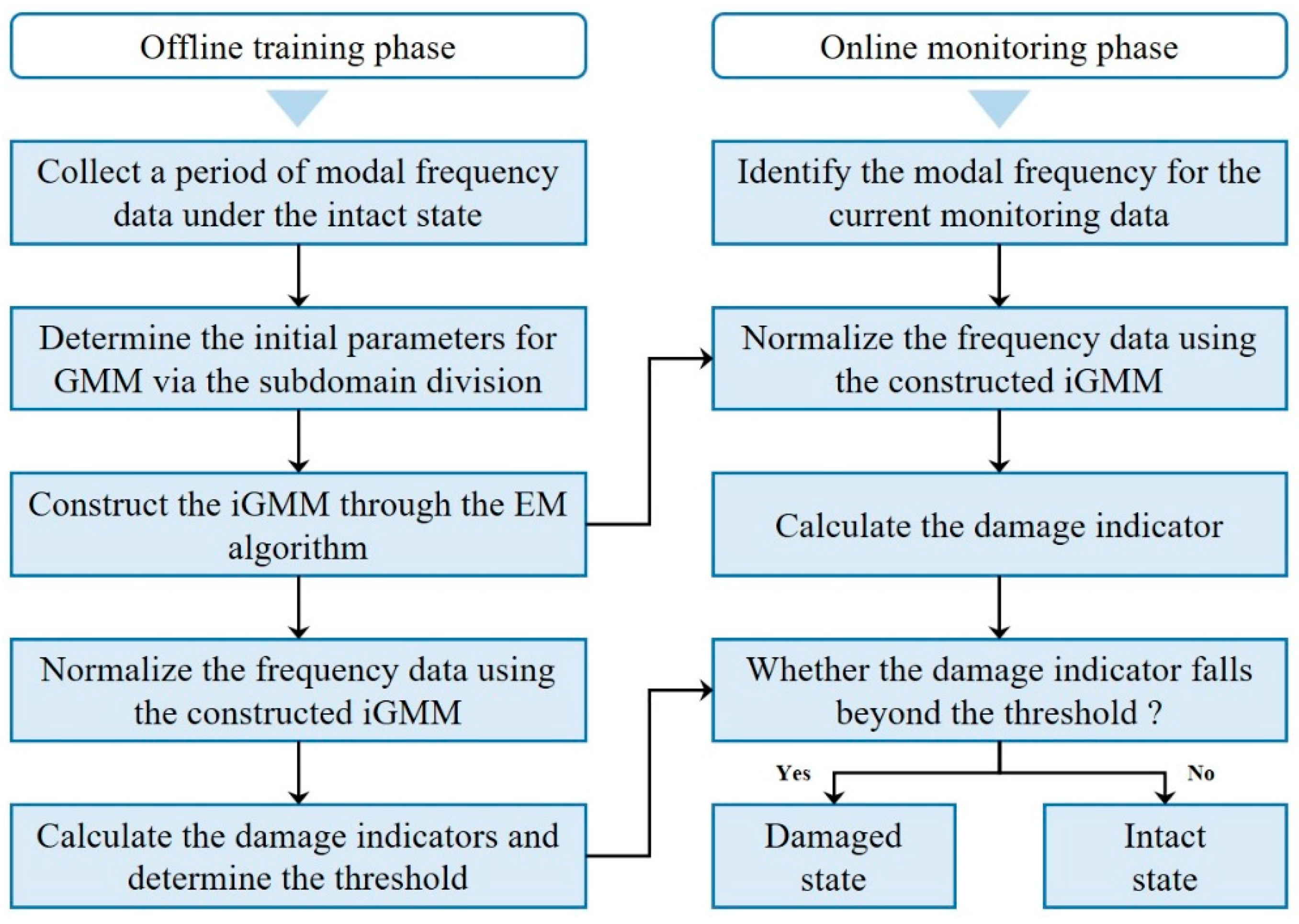
2.5. Implementation Procedure

This iGMM-based damage detection approach consists of two key phases: offline training and online monitoring. In the offline training phase, a period (e.g., one year) of modal frequency data under the intact state of the monitored structure is collected for iGMM construction, data normalization, damage indicator calculation and damage threshold determination. In the online monitoring phase, the currently identified modal frequency data is first normalized for calculating a damage indicator which is then used to compare with the damage threshold to assess if the monitored structure is damaged. The specific flowchart is shown in Figure 1.

3. Case Studies

Two case studies are conducted in this section to evaluate the iGMM-based damage detection method. The first study examines a numerical mass-spring system where stiffness changes nonlinearly with temperature. The second study uses the Z24 Bridge benchmark model, a well-established reference in the SHM field. In both cases, the structure suffered significant damage, and the sensitivity of the natural frequency changes caused by the damage was less affected by the sensor position. For example, when using modal shapes to determine damage, if the measuring point is far away from the wave, information acquisition will be poor, while the natural frequency has a certain advantage in obtaining global information. Therefore, long-term modal frequency data serve as damage-sensitive indicators to verify the method’s effectiveness.

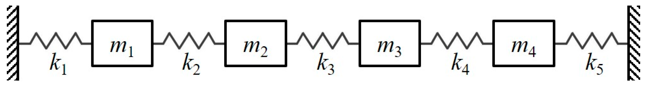
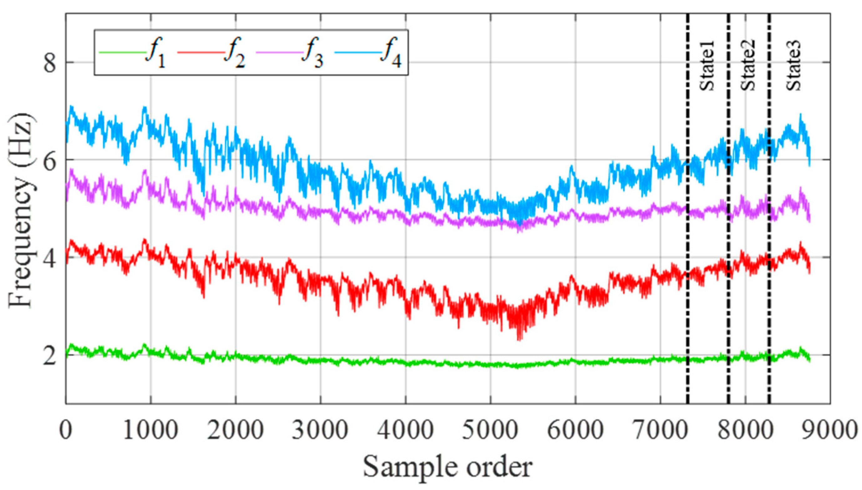
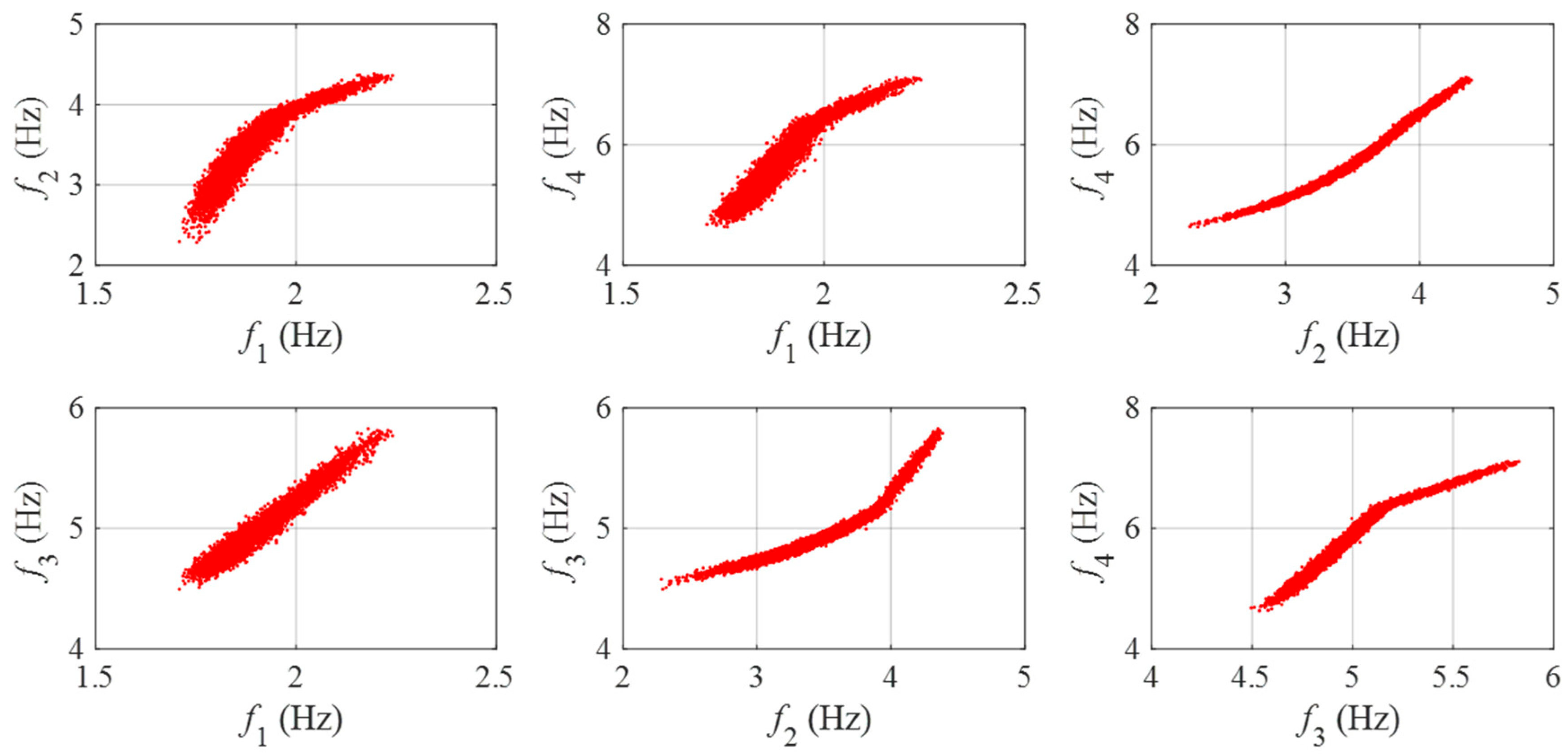
3.1. Case Study Using Numerical Simulation

A four-degree-of-freedom (DOF) mass-spring system, illustrated in Figure 2, is analyzed to validate the effectiveness of the proposed iGMM-based damage detection method. In this system, both ends are fixed to the ground, and each lumped mass has a weight of 2 kg. The nonlinear influence of environmental changes is simulated by defining the functional dependence of stiffness on temperature as shown below [38,51]:

$$k_1=k_2=k_4=k_5=\left\{\begin{array}{ccc}-0.15\times T+8& \mathrm{i}\mathrm{f}& T<0\\ -0.05\times T+8& \mathrm{i}\mathrm{f}& T\ge 0\end{array}\right.$$

(20)

$$k_3=\left\{\begin{array}{ccc}-0.15\times T+10& \mathrm{i}\mathrm{f}& T<0\\ -0.25\times T+10& \mathrm{i}\mathrm{f}& T\ge 0\end{array}\right.$$

(21)

where $T$ represents the temperature.

A total of 8760 h continuous air temperature monitoring records [51,52], as shown in Figure 3, were used for the numerical simulation of modal frequencies. To simulate damage, the stiffness of the second spring $k_2$ was reduced. Three scenarios were considered: for damage state 1, a 10% reduction occurred over data points 7321 and 7800, for damage state 2, a 20% reduction was applied over data points 7801 and 8280, and for damage state 3, a 30% reduction was introduced over data points 8281 and 8760. For each temperature, the equations of motion were solved to obtain the four modal frequencies of the mass-spring system. To account for measurement errors, a small amount of Gaussian white noise ($\mathcal{N}\left(0,0.02\right)$) was incorporated into the modal frequency data. The four time series of simulated modal frequencies are illustrated in Figure 4, where the dashed vertical lines mark the onset of the three damage states. As shown in the figure, temperature variations result in pronounced nonstationary fluctuations in modal frequencies. Because these temperature-induced fluctuations are greater in magnitude than those from stiffness loss, the simulated damages in the mass-spring system cannot be detected by observing modal frequency changes alone.

In order to further understand the simulated modal frequencies, the scatter diagrams representing the mutual correlations between modal frequencies (in the intact state of the mass-spring system) are presented in Figure 5. The figure clearly shows that, except for the correlation between the first and third modal frequencies, the relationships between modal frequencies are nonlinear due to the nonlinear behavior of the third spring. Additionally, the degree of nonlinearity varies among different modal frequency pairs.

In the intact condition, 80% of the modal frequency data (5856 samples) were randomly chosen as the training dataset, with the remaining 20% (1464 samples) allocated to the test set. For the damaged state, all 1440 modal frequency samples were included in the test dataset.

The GLRT-based subdomain division strategy was employed to determine the initial parameter values of GMM. Each training data vector’s 2-norm was calculated, and the dataset was subsequently arranged in ascending order according to these computed norms. In this numerical example, the optimal construction of the iGMM was achieved with a sliding window size equal to 14% of the total training sample count. The iGMM was then applied to normalize both the training and test datasets. Figure 6 displays the four normalized modal frequencies from these datasets, with the three dashed vertical lines marking the starting points of the respective damage states. Compared with Figure 4, it can be clearly seen from Figure 6 that the normalized modal frequency data in the intact state becomes very stationary, and there is an obvious difference between the normalized modal frequencies in the damaged state and the normalized modal frequencies in the intact state. These results demonstrate that the iGMM-based data normalization process is capable of removing the environmental effects on structural damage detection. Moreover, the scatter diagrams representing the mutual correlations between the normalized modal frequencies in the intact state are shown in Figure 7. Compared with Figure 5, it can be clearly seen from Figure 7 that the mutual correlations between the normalized modal frequencies become more linear.

The cumulative T² statistics were calculated for the normalized modal frequencies in both the training and test datasets to demonstrate the damage detection performance of the proposed method. The damage detection results using the cumulative T² statistics with $s=1$, $s=2$, $s=3$ and $s=4$ are, respectively, shown in Figure 8. It can be clearly seen that rare damage indicators fall beyond their corresponding thresholds when the mass-spring system is in an intact state, there is a tendency for the damage indicators to increase as the damage level increases, and more and more damaged samples are successfully detected as the number of consecutive samples used to calculate the cumulative statistics increases. The damage detection rates corresponding to Figure 8 are calculated and listed in

Table 1. Damage detection rates for the mass-spring system.

Cumulative Statistic	Damage Detection Rate (%)
	Training	Test (Intact)	Test (Damage 1)	Test (Damage 2)	Test (Damage 3)
$s=1$	0.31	0.20	42.71	70.42	91.46
$s=2$	0.24	0.20	81.88	93.96	100
$s=3$	0.26	0.34	93.54	99.58	100
$s=4$	0.27	0.34	96.04	100	100

. It is seen that the false alarm rates are very low for all the damage indicators when the mass-spring system is in the intact state, and the damage indicator with $s=4$ is capable of detecting the three levels of damage when the mass-spring system is in the damaged state.

3.2. Case Study Using the Z24 Bridge Data

This study utilized real frequency data obtained from the Z24 Bridge to validate the effectiveness of the proposed iGMM-based damage detection method. Shown in Figure 9, the Z24 Bridge was a prestressed concrete highway bridge situated in the Bern region of Switzerland. The bridge was removed at the end of 1998 to make way for a wider structure to meet traffic requirements. Prior to its demolition, it was monitored extensively for almost a year [13,44,47], with measurements including vibrations and environmental conditions. Furthermore, several types of damage were deliberately applied to support SHM verification efforts.

Using stochastic subspace identification, the first four modal frequencies were derived from the vibration data of the Z24 Bridge. Preprocessing eliminated missing samples from the original dataset, resulting in a time series of 3932 samples, as illustrated in Figure 10. The dashed vertical line represents the point where damage begins. The fluctuations in modal frequencies, primarily due to environmental factors, are pronounced and overshadow the relative changes caused by damage. This makes it challenging to differentiate between the intact and damaged states, highlighting the need to eliminate environmental effects.

The scatter plots in Figure 11 depict the mutual correlations among modal frequencies in the intact state of the Z24 Bridge. Similar to the 4-DOF mass-spring system, nonlinear interactions are evident, especially between the second modal frequency and one of the remaining three frequencies.

The dataset consists of 3932 modal frequency samples, with 3470 belonging to the intact state and 462 to the damaged state. In the intact state, 2776 samples (80%) were randomly selected for training, while the remaining 694 samples (20%) were added to the test dataset. All 462 samples collected from the damaged state were used as an additional part of the test dataset.

Similar to the numerical case study, the GLRT-based subdomain division strategy was employed to determine the initial parameter values of GMM. Each training data vector’s 2-norm was calculated, and the training dataset was reordered in ascending order accordingly. In this real-world case, the iGMM achieved optimal construction when the sliding window size was 11% of the total training dataset. The iGMM was subsequently used to normalize both training and test datasets. Figure 12 illustrates the four normalized modal frequencies, with the dashed vertical line indicating the damage onset. Compared with Figure 10, it can be clearly seen from Figure 12 that the normalized modal frequency data in the intact state becomes stationary, and there is an obvious difference between the normalized modal frequencies in the damaged state and the normalized modal frequencies in the intact state. These results demonstrate that the iGMM-based data normalization process is capable of removing the environmental effects on structural damage detection. Moreover, the scatter diagrams representing the mutual correlations between the normalized modal frequencies in the intact state are shown in Figure 13. Compared with Figure 11, it can be clearly seen from Figure 13 that the mutual correlations between the normalized modal frequencies become more linear.

In order to demonstrate the performance of the proposed method, the cumulative T² statistics were calculated for the normalized modal frequencies in both the training and test datasets. The damage detection results using the cumulative T² statistics with $s=1$ and $s=2$ are, respectively, shown in Figure 14. In the image, the point above the threshold red line indicates recognition as damage, while the point below the threshold red line indicates unrecognized damage. The left side of the vertical black dashed line is in an undamaged state, and the right side of the vertical black dashed line is in a damaged state. It is seen that rare damage indicators fall beyond their corresponding thresholds when the Z24 Bridge is in an intact state and more damaged samples are successfully detected as the number of consecutive samples used to calculate the cumulative statistics increases. The damage detection rates corresponding to Figure 14 are calculated and listed in

Table 2. Damage detection rates for the Z24 Bridge.

Cumulative Statistic	Damage Detection Rate (%)
	Training	Test (Intact State)	Test (Damaged State)
$s=1$	0.29	0.14	96.32
$s=2$	0.29	0.00	98.92

. It can be seen that the false alarm rates are very low for all the damage indicators when the Z24 Bridge is in the intact state. Comparing the false alarm rates in the test and training sets under two different scenarios, the values of the two are very close, indicating that the proposed method has a good generalization of the model. In addition, when the Z24 bridge is in a damaged state, the damage indicator can effectively detect the damage to the bridge, and the damage recognition rate in both cases ($s=1$ or $s=2$) is greater than 96%.

Since other GMM-based damage detection methods [3,36,38,39] were tested on the Z24 Bridge, we compared their performance with that of the proposed method. The results show that the proposed method surpasses references [3,36] in terms of both detection rate and false alarm reduction. Additionally, while the detection rates in references [37,38] are comparable to those of the proposed method, their thresholds appear overly restrictive, leading to a higher number of false alarms.

4. Conclusions

Widely employed for assessing structural conditions, modal frequencies are sensitive to damage but are also highly influenced by environmental changes. To enable damage detection immune to such influences, this study proposes an iGMM-based approach for normalizing modal frequency data. Two case studies were conducted to validate the method, and the following conclusions were drawn:

(1) The traditional GMM construction results largely depend on the initial parameter values provided for the EM algorithm, and there is a high degree of uncertainty. To this end, a subdomain partitioning strategy was proposed to determine the unique initial parameters for constructing iGMM, using sliding window and generalized likelihood ratio test methods. Then, using the EM algorithm, GMM is constructed simply and effectively based on the previously determined initial parameters.

(2) Environmental changes can introduce nonstationary and nonlinear variations in structural modal frequencies, which significantly reduce the effectiveness of damage detection based on direct observation of frequency changes. However, based on the iGMM, the normalized modal frequencies were no longer affected by the environmental changes and exhibited distinguishability between the intact and damaged states of structures.

(3) Hotelling’s T² statistic and its cumulative form of the normalized modal frequencies were defined as damage indicators; meanwhile, the corresponding damage thresholds were determined according to the kernel density estimation technique. The case studies demonstrated that the cumulative statistic is able to serve as an excellent damage indicator in terms of SHM.

References

1. Avci, O.; Abdeljaber, O.; Kiranyaz, S.; Hussein, M.; Gabbouj, M.; Inman, D.J. A review of vibration-based damage detection in civil structures: From traditional methods to machine learning and deep learning applications. Mech. Syst. Signal Process. 2021, 147, 107077. [Google Scholar] [CrossRef]
2. Hou, R.; Xia, Y. Review on the new development of vibration-based damage identification for civil engineering structures: 2010–2019. J. Sound Vib. 2021, 491, 115741. [Google Scholar] [CrossRef]
3. Xiao, F.; Mao, Y.; Sun, H.; Chen, G.S.; Tian, G. Stiffness Separation Method for Reducing Calculation Time of Truss Structure Damage Identification. Struct. Control Health Monit. 2024, 2024, 5171542. [Google Scholar] [CrossRef]
4. Xiao, F.; Mao, Y.; Tian, G.; Chen, G.S. Partial-Model-Based Damage Identification of Long-Span Steel Truss Bridge Based on Stiffness Separation Method. Struct. Control Health Monit. 2024, 2024, 5530300. [Google Scholar] [CrossRef]
5. Xiao, F.; Sun, H.; Mao, Y.; Chen, G.S. Damage identification of large-scale space truss structures based on stiffness separation method. Structures 2023, 53, 109–118. [Google Scholar] [CrossRef]
6. Figueiredo, E.; Radu, L.; Worden, K.; Farrar, C.R. A Bayesian approach based on a Markov-chain Monte Carlo method for damage detection under unknown sources of variability. Eng. Struct. 2014, 80, 1–10. [Google Scholar] [CrossRef]
7. Ubertini, F.; Comanducci, G.; Cavalagli, N. Vibration-based structural health monitoring of a historic bell-tower using output-only measurements and multivariate statistical analysis. Struct. Health Monit. 2016, 15, 438–457. [Google Scholar] [CrossRef]
8. Cantero, D.; Hester, D.; Brownjohn, J. Evolution of bridge frequencies and modes of vibration during truck passage. Eng. Struct. 2017, 152, 452–464. [Google Scholar] [CrossRef]
9. Roy, K.; Samit, R.C. Fundamental mode shape and its derivatives in structural damage localization. J. Sound Vib. 2013, 332, 5584–5593. [Google Scholar] [CrossRef]
10. Frigui, F.; Faye, J.P.; Martin, C.; Dalverny, O.; Peres, F.; Judenherc, S. Global methodology for damage detection and localization in civil engineering structures. Eng. Struct. 2018, 171, 686–695. [Google Scholar] [CrossRef]
11. Cui, H.Y.; Xu, X.; Peng, W.Q.; Zhou, Z.; Hong, M. A damage detection method based on strain modes for structures under ambient excitation. Measurement 2018, 125, 438–446. [Google Scholar] [CrossRef]
12. Bhuyan, M.D.H.; Gautier, G.; Le Touz, N.; Döhler, M.; Hille, F.; Dumoulin, J.; Mevel, L. Vibration-based damage localization with load vectors under temperature changes. Struct. Control Health Monit. 2019, 26, e2439. [Google Scholar] [CrossRef]
13. Wah, W.S.L.; Chen, Y.T.; Owen, J.S. A regression-based damage detection method for structures subjected to changing environmental and operational conditions. Eng. Struct. 2021, 228, 111462. [Google Scholar]
14. Liu, C.; DeWolf, J.T. Effect of temperature on modal variability of a curved concrete bridge under ambient loads. J. Struct. Eng. 2007, 133, 1742–1751. [Google Scholar] [CrossRef]
15. Kim, J.T.; Park, J.H.; Lee, B.J. Vibration-based damage monitoring in model plate-girder bridges under uncertain temperature conditions. Eng. Struct. 2007, 29, 1354–1365. [Google Scholar] [CrossRef]
16. Cross, E.J.; Koo, K.Y.; Brownjohn, J.M.W.; Worden, K. Long-term monitoring and data analysis of the Tamar Bridge. Mech. Syst. Signal Process. 2013, 35, 16–34. [Google Scholar] [CrossRef]
17. Han, Q.; Ma, Q.; Xu, J.; Liu, M. Structural health monitoring research under varying temperature condition: A review. J. Civ. Struct. Health Monit. 2021, 11, 149–173. [Google Scholar] [CrossRef]
18. Wang, Z.; Yang, D.H.; Yi, T.H.; Zhang, G.H.; Han, J.G. Eliminating environmental and operational effects on structural modal frequency: A comprehensive review. Struct. Control Health Monit. 2022, 29, e3073. [Google Scholar] [CrossRef]
19. Peeters, B.; De Roeck, G. One-year monitoring of the Z24-Bridge: Environmental effects versus damage events. Earthq. Eng. Struct. Dyn. 2001, 30, 149–171. [Google Scholar] [CrossRef]
20. Moser, P.; Moaveni, B. Environmental effects on the identified natural frequencies of the Dowling Hall Footbridge. Mech. Syst. Signal Process. 2011, 25, 2336–2357. [Google Scholar] [CrossRef]
21. Hu, W.H.; Cunha, A.; Caetano, E.; Rohrmann, R.G.; Said, S.; Teng, J. Comparison of different statistical approaches for removing environmental/operational effects for massive data continuously collected from footbridges. Struct. Control Health Monit. 2017, 24, e1955. [Google Scholar] [CrossRef]
22. Ni, Y.Q.; Zhou, H.F.; Ko, J.M. Generalization capability of neural network models for temperature-frequency correlation using monitoring data. J. Struct. Eng. 2009, 135, 1290–1300. [Google Scholar] [CrossRef]
23. Worden, K.; Cross, E.J. On switching response surface models, with applications to the structural health monitoring of bridges. Mech. Syst. Signal Process. 2018, 98, 139–156. [Google Scholar] [CrossRef]
24. Ma, K.C.; Yi, T.H.; Yang, D.H.; Li, H.N.; Liu, H. Multiorder detection of bridge modal-frequency anomalies considering multiple environmental factors. J. Perform. Constr. Facil. 2022, 36, 04022046. [Google Scholar] [CrossRef]
25. Prawin, J.; Lakshmi, K.; Rao, A.R.M. Structural damage diagnosis under varying environmental conditions with very limited measurements. J. Intell. Mater. Syst. Struct. 2020, 31, 665–686. [Google Scholar] [CrossRef]
26. Yan, A.M.; Kerschen, G.; De Boe, P.; Golinval, J.C. Structural damage diagnosis under varying environmental conditions—Part I: A linear analysis. Mech. Syst. Signal Process. 2005, 19, 847–864. [Google Scholar] [CrossRef]
27. Sen, D.; Erazo, K.; Zhang, W.; Nagarajaiah, S.; Sun, L. On the effectiveness of principal component analysis for decoupling structural damage and environmental effects in bridge structures. J. Sound Vib. 2019, 457, 280–298. [Google Scholar] [CrossRef]
28. Yan, A.M.; Kerschen, G.; De Boe, P.; Golinval, J.C. Structural damage diagnosis under varying environmental conditions—Part II: Local PCA for non-linear cases. Mech. Syst. Signal Process. 2005, 19, 865–880. [Google Scholar] [CrossRef]
29. Zhou, H.F.; Ni, Y.Q.; Ko, J.M. Structural damage alarming using auto-associative neural network technique: Exploration of environment-tolerant capacity and setup of alarming threshold. Mech. Syst. Signal Process. 2011, 25, 1508–1526. [Google Scholar] [CrossRef]
30. Ozdagli, A.I.; Koutsoukos, X. Machine learning based novelty detection using modal analysis. Comput.-Aided Civ. Infrastruct. Eng. 2019, 34, 1119–1140. [Google Scholar] [CrossRef]
31. Maes, K.; Van Meerbeeck, L.; Reynders, E.P.B.; Lombaert, G. Validation of vibration-based structural health monitoring on retrofitted railway bridge KW51. Mech. Syst. Signal Process. 2022, 165, 108380. [Google Scholar] [CrossRef]
32. Cross, E.J.; Worden, K.; Chen, Q. Cointegration: A novel approach for the removal of environmental trends in structural health monitoring data. Proc. R. Soc. A 2011, 467, 2712–2732. [Google Scholar] [CrossRef]
33. Worden, K.; Cross, E.J.; Antoniadou, I.; Kyprianou, A. A multiresolution approach to cointegration for enhanced SHM of structures under varying conditions–an exploratory study. Mech. Syst. Signal Process. 2014, 47, 243–262. [Google Scholar] [CrossRef]
34. Mousavi, M.; Gandomi, A.H. Prediction error of Johansen cointegration residuals for structural health monitoring. Mech. Syst. Signal Process. 2021, 160, 107847. [Google Scholar] [CrossRef]
35. Dervilis, N.; Antoniadou, I.; Cross, E.J.; Worden, K. A non-linear manifold strategy for SHM approaches. Strain 2015, 51, 324–331. [Google Scholar] [CrossRef]
36. Peng, Z.; Li, J.; Hao, H. Structural damage detection via phase space based manifold learning under changing environmental and operational conditions. Eng. Struct. 2022, 263, 114420. [Google Scholar] [CrossRef]
37. Zang, J.G.; Huang, H.B.; Sun, Z.G.; Wang, D.S. Subdomain principal component analysis for damage detection of structures subjected to changing environments. Eng. Struct. 2023, 288, 116265. [Google Scholar] [CrossRef]
38. Shi, H.; Worden, K.; Cross, E.J. A regime-switching cointegration approach for removing environmental and operational variations in structural health monitoring. Mech. Syst. Signal Process. 2018, 103, 381–397. [Google Scholar] [CrossRef]
39. Wang, Z.; Yi, T.H.; Yang, D.H.; Zhou, P.; Sun, L. Early warning method of structural damage using localized frequency cointegration under changing environments. J. Struct. Eng. 2023, 149, 04022230. [Google Scholar] [CrossRef]
40. Huang, J.Z.; Li, D.S.; Li, H.N. A new regime-switching cointegration method for structural health monitoring under changing environmental and operational conditions. Measurement 2023, 212, 112682. [Google Scholar] [CrossRef]
41. Huang, J.Z.; Yuan, S.J.; Li, D.S.; Li, H.N. A kernel canonical correlation analysis approach for removing environmental and operational variations for structural damage identification. J. Sound Vib. 2023, 548, 117516. [Google Scholar] [CrossRef]
42. Kullaa, J. Structural health monitoring under nonlinear environmental or operational influences. Shock Vib. 2014, 2014, 863494. [Google Scholar] [CrossRef]
43. Figueiredo, M.A.T.; Jain, A.K. Unsupervised learning of finite mixture models. IEEE Trans. Pattern Anal. Mach. Intell. 2002, 24, 381–396. [Google Scholar] [CrossRef]
44. Santos, A.; Silva, M.; Santos, R.; Figueiredo, E.; Sales, C.; Costa, J.C. A global expectation-maximization based on memetic swarm optimization for structural damage detection. Struct. Health Monit. 2016, 15, 610–625. [Google Scholar] [CrossRef]
45. Santos, A.; Figueiredo, E.; Silva, M.; Santos, R.; Sales, C.; Costa, J.C. Genetic-based EM algorithm to improve the robustness of Gaussian mixture models for damage detection in bridges. Struct. Control Health Monit. 2017, 24, e1886. [Google Scholar] [CrossRef]
46. Qiu, L.; Fang, F.; Yuan, S. Improved density peak clustering-based adaptive Gaussian mixture model for damage monitoring in aircraft structures under time-varying conditions. Mech. Syst. Signal Process. 2019, 126, 281–304. [Google Scholar] [CrossRef]
47. Cubedo, M.; Oller, J.M. Hypothesis testing: A model selection approach. J. Stat. Plan. Inference 2002, 108, 3–21. [Google Scholar] [CrossRef]
48. Verbeek, J.J.; Vlassis, N.; Kröse, B. Efficient greedy learning of Gaussian mixture models. Neural Comput. 2003, 15, 469–485. [Google Scholar] [CrossRef] [PubMed]
49. Pernkopf, F.; Bouchaffra, D. Genetic-based EM algorithm for learning Gaussian mixture models. IEEE Trans. Pattern Anal. Mach. Intell. 2005, 27, 1344–1348. [Google Scholar] [CrossRef] [PubMed]
50. Huang, H.B.; Yi, T.H.; Li, H.N.; Liu, H. New representative temperature for performance alarming of bridge expansion joints through temperature-displacement relationship. J. Bridge Eng. 2018, 23, 04018043. [Google Scholar] [CrossRef]
51. Pei, X.Y.; Zhang, H.T.; Huang, H.B.; Liang, D. Probabilistic machine learning-based frequency normalization method for bridge damage detection considering environmental variations. Int. J. Struct. Stab. Dyn. 2024. [Google Scholar] [CrossRef]
52. Huang, H.B.; Yi, T.H.; Li, H.N.; Liu, H. Sparse Bayesian identification of temperature-displacement model for performance assessment and early warning of bridge bearings. J. Struct. Eng. 2022, 148, 04022052. [Google Scholar] [CrossRef]
Figure 1. Flowchart describing the implementation procedure of the proposed method.
Buildings 15 00359 g001
Figure 2. The 4-DOF mass-spring system.
Buildings 15 00359 g002
Figure 3. Air temperature monitoring records used for numerical simulation of the mass-spring system.
Buildings 15 00359 g003
Figure 4. The four modal frequency time series simulated for the mass-spring system.
Buildings 15 00359 g004
Figure 5. Scatter diagrams representing the mutual correlations between simulated modal frequencies of the mass-spring system.
Buildings 15 00359 g005
Figure 6. The four normalized modal frequencies for the mass-spring system.
Buildings 15 00359 g006aBuildings 15 00359 g006b
Figure 7. Scatter diagrams representing the mutual correlations between normalized modal frequencies of the mass-spring system.
Buildings 15 00359 g007
Figure 8. Damage detection results for the mass-spring system.
Buildings 15 00359 g008
Figure 9. The Z24 Bridge [17,44]: (a) longitudinal section, (b) top view, (c) cross section.
Buildings 15 00359 g009
Figure 10. The first four modal frequency time series identified for the Z24 Bridge.
Buildings 15 00359 g010
Figure 11. Scatter diagrams representing the mutual correlations between modal frequencies of the Z24 Bridge.
Buildings 15 00359 g011
Figure 12. The four normalized modal frequencies for the Z24 Bridge.
Buildings 15 00359 g012aBuildings 15 00359 g012b
Figure 13. Scatter diagrams representing the mutual correlations between normalized modal frequencies of the Z24 Bridge.
Buildings 15 00359 g013
Figure 14. Damage detection results for the Z24 Bridge.
Buildings 15 00359 g014