Probabilistic Analysis of Creep and Shrinkage Effects on Prestressed Concrete Bridges Using Solid Element Models

Abstract

Concrete creep and shrinkage are critical factors affecting the long-term performance of extradosed bridges, leading to deflection, stress redistribution, and potential cracking. Predicting these effects is challenging due to uncertainties in empirical models and a lack of long-term data. While beam element models are common in design, they often fail to capture complex stress fields in disturbed regions (D-regions), potentially leading to non-conservative assessments of crack resistance. This study presents a computationally efficient probabilistic framework that integrates the First-Order Second-Moment (FOSM) method with a high-fidelity solid element model to analyze these time-dependent effects. Our analysis reveals that solid element models predict 14% higher long-term deflections and 64% greater sensitivity to creep and shrinkage parameters compared to beam models, which underestimate both the mean and variability of deformation. The FOSM-based framework proves highly efficient, with its prediction for the standard deviations of bridge deflection falling within 7.1% of those from the more computationally intensive Probability Density Evolution Method. Furthermore, we found that time-varying parameters have a minimal effect on principal stress directions, validating a scalar application of FOSM with less than 3% error. The analysis shows that uncertainties from creep and shrinkage models increase the 95% quantile of in-plane principal stresses by 0.58MPa, which is approximately 23% of the material’s tensile strength and increases the cracking risk. This research underscores the necessity of using high-fidelity models and probabilistic methods for the reliable design and long-term assessment of complex concrete bridges.

1. Introduction

Prestressed concrete bridges are profoundly influenced by time-dependent phenomena such as creep and shrinkage, which can significantly impact their serviceability and safety [1]. These effects, often underestimated in initial design phases, can culminate in notable structural consequences over decades, including excessive deflection, cracking, undesirable redistribution of internal forces, and even serviceability or safety failures.

In prestressed concrete members, creep and shrinkage are major contributors to the long-term loss of prestress, compromising their intended performance. These effects are particularly critical in complex systems like cable-stayed bridges and extradosed bridges, where the precise prediction of long-term behavior is essential for ensuring structural integrity and preventing serviceability failures.

The uncertainty inherent in predicting creep and shrinkage poses a formidable challenge in structural reliability analysis. Numerous prediction models, such as ACI 209R, CEB-FIP, and B3/B4 model, have been developed, yet they often yield disparate results due to differing assumptions and parametric sensitivities [2]. A critical limitation is the severe scarcity of multi-decade experimental data, with 96% of all available laboratory data not exceeding 6 years in duration, which forces models to extrapolate far beyond their validated ranges and introduces significant uncertainty into long-term predictions [2]. Even with laboratory-measured data, there is inherent variability (e.g., approximately an 8% coefficient of variation for shrinkage within a single concrete mixture), meaning that these models cannot perfectly match experimental data [1]. Comparative studies show no single model consistently outperforms others across all concrete types and conditions [3]. For instance, the GL2000 model was found to be the closest to experimental results in one study [4], while the CEB-FIP (1970) and BS 8110 (1985) methods provided suitably accurate predictions in another [5]. This variability necessitates robust probabilistic approaches to quantify the impact of these uncertainties and ensure that safety margins are adequate throughout a structure’s design life. Consequently, the focus of advanced analysis has shifted from deterministic predictions to stochastic frameworks that can account for the random nature of material properties and model inaccuracies [6].

Initial frameworks for time-dependent reliability analysis often paired methods like the First-Order Reliability Method (FORM) [7] with simplified structural representations, such as beam elements. However, in disturbed regions (D-regions)—defined near abrupt changes in geometry or locations of concentrated forces [8]—the strain distribution becomes highly nonlinear compared with the idealized linear strain assumption of beam theory. The accurate analysis of D-regions therefore requires a refined finite element approach capable of capturing complex stress and strain fields. While foundational, these approaches cannot capture the complex stress fields in disturbed regions (D-regions), like girder webs near tendon anchorages, where the plane sections assumption is invalid [9,10,11]. Numerous studies have highlighted the limitations of beam element models in capturing complex stress states in D-regions [9,10,11]. Deterministic studies have identified significant discrepancies in stress and deformation predictions between beam and solid element models, particularly in regions with geometric discontinuities or concentrated forces [12,13]. These discrepancies underscore that beam models can significantly underestimate stress concentrations and misrepresent structural behavior in these critical zones, potentially leading to non-conservative designs [12,13]. Solid elements, which provide a high-fidelity representation of the structural geometry, are crucial for accurately capturing these non-linear stress distributions and localized stress concentrations.

Although more sophisticated probabilistic techniques have emerged—including the Probability Density Evolution Method (PDEM) [6] and surrogate models like Polynomial Chaos Expansion (PCE) [14] or Kriging [15]—their application has been constrained by a persistent trade-off between model fidelity and computational cost. The immense computational expense of running thousands of simulations, particularly with high-fidelity Finite Element Analysis (FEA) using solid elements, has largely restricted these powerful methods to simpler beam or grillage models [16,17,18]. This leaves a critical gap in the probabilistic analysis of high-fidelity solid element models.

Furthermore, while some studies have explored general model uncertainties, few have comprehensively quantified the impact of different creep and shrinkage models on critical structural responses like principal stresses and long-term deflections in a probabilistic context, especially for complex structures analyzed with solid elements [19,20,21,22,23]. This gap is significant given the known variability of these models’ predictions.

This study aims to bridge these gaps by developing and applying a computationally efficient probabilistic framework to analyze the long-term effects of creep and shrinkage on an extradosed bridge using a detailed solid element model. The paper introduces a methodology that integrates the First-Order Second-Moment (FOSM) method with high-fidelity finite element analysis, making a rigorous probabilistic assessment of complex D-regions computationally feasible. Furthermore, we propose a novel and validated approach for the probabilistic analysis of principal stresses that correctly accounts for the variability of the entire stress state. Finally, the analysis evaluates the impact of uncertainties from four different creep and shrinkage models, providing crucial data on how model selection affects the operational cracking risk and compressive stress reserves in critical structural elements [24].

Therefore, the main purpose of this research is not only to improve the estimation of long-term creep and shrinkage effects but also to provide a practical and accurate pathway for full-bridge uncertainty analysis using solid elements, bridging the long-standing gap between model fidelity and computational feasibility.

2. Probabilistic Analysis Methods

Traditional Monte Carlo methods require a large number of random samples to achieve high accuracy. The sample size grows exponentially with the number of variables, resulting in high computational costs. This paper employs the First-Order Second-Moment (FOSM) method for the probabilistic analysis of shrinkage and creep effects. To validate this computationally efficient approach, its results are compared against those from a more rigorous low-discrepancy quasi-Monte Carlo sampling method based on number theory.

2.1. Quasi-Monte Carlo Sampling

The number-theoretic method is particularly effective to high-dimensional variables with significantly reduced number of samples [6]. The basic idea is to generate a set of uniformly distributed points in an s-dimensional space using the consistent distribution point set proposed by Fang and Wang [25]. For an s-dimensional random variable (${\tilde{X}}_1,{\tilde{X}}_2,\dots ,{\tilde{X}}_s)$ located in the unit hypercube $[0,1{]}^s$, the coordinates of the k-th sample point ${\mathit{x}}_{\mathit{k}}$ are given by:

$${\tilde{\mathit{x}}}_{\mathit{k}}=\left(x_{1k},x_{2k},\dots ,x_{sk}\right)=\left({\displaystyle \frac{h_{1}k-0.5}{n}},\left\{{\displaystyle \frac{h_{2}k-0.5}{n}}\right\},\dots ,\left\{{\displaystyle \frac{h_{s}k-0.5}{n}}\right\}\right)$$

(1)

with

$$\left\{{\displaystyle \frac{h_{s}k-0.5}{n}}\right\}={\displaystyle \frac{h_{s}k-0.5}{n}}-⌊{\displaystyle \frac{h_{s}k-0.5}{n}}⌋$$

(2)

where the parameters $h_1$, $h_2,\dots ,h_s$ can be found in the appendix of reference [25] based on the number of random variables, s. Here, N is the total number of sample points, which is also determined from a table in reference [25] based on the number of random variables s. The operator ⌊⋅⌋ denotes the greatest integer not exceeding the number inside the brackets.

A key characteristic of the number-theoretic method is that the generated sample points are not equiprobable. Instead, the probability $P_{{\mathit{x}}_{\mathit{k}}}$ associated with each point ${\mathit{x}}_{\mathit{k}}$ is determined by its position within the target distribution space. Therefore, an inverse Cumulative Distribution Function (CDF) transformation is not necessary. The subsequent statistical calculations, as detailed in Equations (5) and (6), directly account for the varying probability of each sample point. This approach is fundamental to the method and is consistent with the procedures outlined in the literature [26,27]. Uniformly distributed sample points from the hypercube are mapped to the target domain of specific random variables through a linear transformation involving scaling and shifting.

In a multi-dimensional Gaussian space, the number of sample points can be further optimized. This approach leverages the property that the joint probability density of a high-dimensional Gaussian distribution is very low near its boundaries. Accordingly, this study screens out low-probability-density sample points that are located outside a hypersphere of radius r by retaining only those samples that satisfy the following equation.

$$\sum _{i=1}^s{{(\tilde{x}}_{i,k}-0.5)}^2\le r^2$$

(3)

Let’s define the relationship between the structural response Z and the random variable X as follows:

$$Z=g\left(X_1,X_2,\dots ,X_s\right)$$

(4)

Based on the probability $P_{{\mathit{x}}_{\mathit{k}}}$ of each sample point ${\mathit{x}}_{\mathit{k}}=\left(x_{1k},x_{2k},\dots ,x_{sk}\right)$, the mean ($g\left({\mu }_{\mathrm{X}1},{\mu }_{\mathrm{X}2},\dots ,{\mu }_{Xn}\right)$) and standard deviation (${\delta }_g$) of the structural response Z can be calculated using the following equations.

$$g\left({\mu }_{X1},{\mu }_{X2},\dots ,{\mu }_{Xn}\right)=\sum _{k=1}^n{P}_{{\mathit{x}}_{\mathit{k}}}·g\left({\mathit{x}}_{\mathit{k}}\right)$$

(5)

$${\delta }_g=\sqrt{\sum _{k=1}^n{P}_{{\mathit{x}}_{\mathit{k}}}{\left(g\left({\mathit{x}}_{\mathit{k}}\right)-g\left({\mu }_{X1},{\mu }_{X2},\dots ,{\mu }_{Xn}\right)\right)}^2}$$

(6)

where ${\mu }_{{\mathrm{X}}_k}$ represents the mean of the random variable ${\mathrm{X}}_k$. Furthermore, the probability density of $\left(\mathit{X}\right)$ can also be obtained using the probability density evolution equation documented in [13].

2.2. First-Order Second-Moment (FOSM) Method

The First-Order Second-Moment (FOSM) method [7] is an approximate method for determining structural reliability. Its principle is to describe the statistical characteristics of a random variable using only its mean (the first-order moment about the origin) and its variance (the second-order central moment). For a nonlinear structural response function, it is linearized at its mean point by

$$Z=g\left({\mu }_{\mathrm{X}1},{\mu }_{\mathrm{X}2},\dots ,{\mu }_{Xn}\right)+\sum _i^s{a}_i·\left(x_i-{\mu }_{X_i}\right)$$

(7)

where $a_i=\partial g/\partial X_i$ is the sensitivity coefficient of the function Z = g(X) to the variable $X_i$.

The sensitivity coefficients $a_i$ can be determined through numerical analysis. By calculating the structural response when the i-th random variable deviates from its mean while all other variables remain at their respective means, the sensitivity coefficient can be found:

$$a_i={\displaystyle \frac{g\left({\mu }_{X1},{\mu }_{X2},\dots ,{\mu }_{Xi}+{∆}_i\dots ,{\mu }_{Xs}\right)-g\left({\mu }_{X1},{\mu }_{X2},\dots ,{\mu }_{Xs}\right)}{{∆}_i}}$$

(8)

In this study, we assume the random variables follow the Gaussian distribution. They can be transformed into a standard normal distribution $X_i^{\ast }={\displaystyle \frac{X_i-{\mu }_{X_i}}{{\delta }_{Xi}}}$, where ${\delta }_{Xi}$ is the standard deviation of $X_i$, and ${∆}_{\mathrm{i}}$ is deviation of the i-th random variable from its mean value. Based on Equation (7), the structural response and its standard deviation are given by

$$Z=g\left({\mu }_{\mathrm{X}1},{\mu }_{\mathrm{X}2},\dots ,{\mu }_{Xn}\right)+{\sum }_i^s{a}_i^{\ast }{x}_i^{\ast }$$

(9)

$${\delta }_Z=\sqrt{{\sum }_{i=1}^n{\left(a_i{\delta }_{X_i}\right)}^2}=\sqrt{{\sum }_{i=1}^n{\left(a_i^{\ast }\right)}^2}$$

(10)

where $a_i^{\ast }=a_i{\delta }_{X_i}$ is the sensitivity coefficient of the structural response Z to the standard normal random variable $X_i^{\ast }$. Its physical meaning is the change in the structural response caused by a one-standard-deviation change of $X_i$. Equation (10) shows that the term ${\left(a_i^{\ast }\right)}^2$ represents the contribution of the i-th random variable to the total variance of the structural response.

3. Case Study: Bridge Modeling and Analysis Parameters

The analysis methods described above were applied to a real-world prestressed concrete extradosed bridge. Two distinct models of the bridge were created: a beam element model and a solid element model. The beam element model was used to compare the two probabilistic analysis methods presented in Section 2. Furthermore, by comparing the results from the beam and solid element models, we analyze the influence of the structural modeling approach on the probabilistic analysis results.

3.1. Bridge Configuration

The case study focuses on a four-span extradosed bridge with spans of (117.5 + 230 + 230 + 117.5) meters and three pylons. All pylons are rooted in the main girder, and the girder is supported by the side piers through bearings while rigidly connected to the middle pier. Due to the symmetry of the structure, only the half-bridge shown in Figure 1 needs to be analyzed.

The main girder has a single-box section with three internal chambers. The depth of the main girder varies from 8.0 m at the abutments to 4.0 m at the middle of the span and side-span supports. The top width of the girder is 41 m with horizontal cantilevers of 8 m at each side. Figure 2 illustrates the cross-section box girder.

Table 1. Cross-section of the girder.

Section ID	0	2	4	6	8	10	12
Distance from the mid-span/m	7	14	22	30	38	46	54
Area/m2	60.21	52.91	48.45	44.51	41.08	38.15	35.73
Moment of inertia/m4	481.7	333.75	258.46	200.78	157.19	124.81	101.4
Section ID	14	16	18	20	22	24	26
Distance from the mid-span/m	62	70	78	86	94	102	110
Area/m2	33.82	32.45	31.81	31.68	31.68	31.68	31.68
Moment of inertia/m4	85.6	78.3	72.8	71.4	71.4	71.4	71.4

provides the area and moment of inertia of the girder sections, while

Table 2. Material properties of the cables, tendons, and concrete.

Material	Modulus of Elasticity /(N/m2)	Mass Density /(kg/m3)	Compressive Strength/(N/m2)	Strength of Steel Strand/(N/m2)	Poisson’s Ratio
Girder, pylon	3.60 × 1010	2.60 × 103	5.6 × 107	-	0.2
Cable	1.95 × 1011	2.45 × 103	-	1.86 × 109	0.3
Tendon	1.95 × 1011	8.00 × 103	-	1.86 × 109	0.3

lists the material properties used in the bridge.

Each pylon is 32.8 m high, and the cross-section of the main pylon measures 5 m in the longitudinal direction and 3 m in the transverse direction (in Figure 3). The area and moment of inertia of the pylon section are 14.5 m² and 30.28 m⁴, respectively.

The cables are fabricated using 15.2 mm diameter strands. Two sizes of cable are used, with 61 and 73 bundles of strands, respectively. The standard strength of the strands is 1860 MPa. The main girder is prestressed using 15.2 mm diameter strands. These strands are arranged in three locations: the web, the top flange, and the bottom flange.

The bridge was built using the cantilever construction method according to the sequence in

Table 3. Construction Sequence of the case bridge.

Construction Stage	Stage Name	Construction Description	Duration (Days)
1	Pier	Construct of All Pier	10
2	Girder Segment 0#	Construct Girder Segment 0#, Temporary Fixation at Girder Bottom	10
		Tensioning Prestressing Tendons for Segment 0#	3
3	Main Tower Construction	Construct Main Tower	3
4~18	Cable-Free Zone: Girder Segments 1#–7#	Construct Girder Segment 1#	5
		Tensioning Prestressing Tendons for Segment 1#	3
19~53	Cable-Supported Zone: Girder Segments 8#–25#	Construct Girder Segment 8#	5
		Tensioning Prestressing Tendons for Segment 8#	3
		Tensioning Stay Cables for Segment 8#	3
54~58	Cable-Free Zone: Girder Segments 26#–27#	Construct Girder Segment 26#	5
		Tensioning Prestressing Tendons for Segment 26#	3
59~60	Side Span Closure Segment	Construct Side Span Closure Segment	5
		Tensioning Closure Segment Tendons	3
61~62	Mid-Span Closure Segment	Construct Mid-Span Closure Segment	5
		Tensioning Closure Segment Tendons	3
63	Bridge Deck Paving	Apply Secondary Dead Load	5
64	Bridge in Service	Long-Term Creep	7400

. As can be seen that the construction sequence of the bridge in Table 3 is as follows: first, the piers are built, followed by the 0# segment (the main girder sections directly above the piers, as shown in Figure 1). Then, segments 1# to 27# are cast using the cantilever method. Once the maximum cantilever state has been reached, the two side span closure segments are cast, followed by the mid-span closure segment.

During the cantilever stage, the bearing plates are fully constrained with no allowance for translation or rotation in any direction. Once the main girder is complete, all bearing plates are permitted to rotate around a horizontal axis. Only the middle bearing plate is restricted from moving along the bridge’s axis, while the others are free to move longitudinally.

3.2. Beam Element Model

The main girders, pylons, and piers of the entire bridge structure were modeled using 501 beam elements. The 216 stay cables are simulated using the truss element. The software MIDAS CIVIL 2024 used in this study is capable of conveniently simulating the effects of prestressing, shrinkage, creep, and the overall construction process. The geometry model using the beam element is shown in Figure 4.

3.3. Solid Element Model

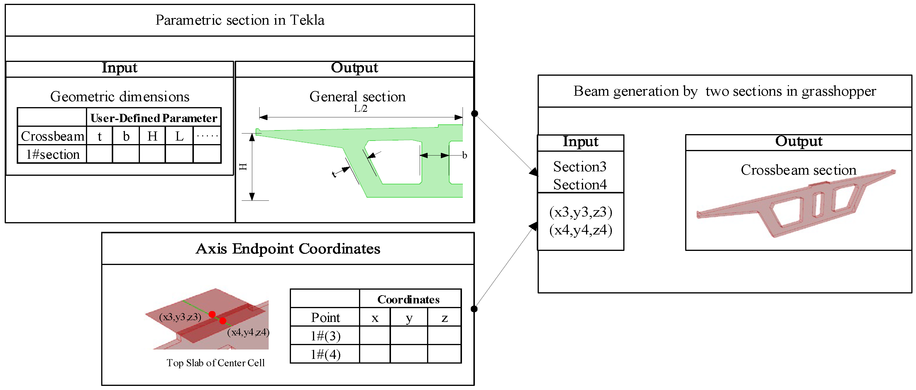
Modeling the bridge in Tekla and Grasshopper automates the creation of complex geometries, such as diaphragms and anchorage blocks for prestressed tendons and stay cables, thereby avoiding the extensive labor costs associated with manual solid modeling.

The box girder’s cross-section is first defined parametrically in Tekla (top-left of Figure 5). These parametric sections are then converted into “section components” in Grasshopper, which are in turn used to create “segment components” via visual programming. As the right side of Figure 5 shows, this program takes four input parameters—the two end “section components” and their global coordinates—to create a segment with a varying cross-section. Diaphragm locations are modeled similarly, by treating the girder segment at the diaphragm as a separate entity where the end sections include diaphragms.

This automated and parametric approach also extends to the geometry of anchorage blocks for prestressed tendons and stay cables. A parametric template defines the block’s geometry, which is then positioned within the local coordinates of the girder segment. The block and girder are then combined into a single solid component using Boolean operations. Similarly, the prestressing tendons’ geometry is parameterized in Grasshopper, using the same input parameters as conventional bridge analysis software like Midas Civil.

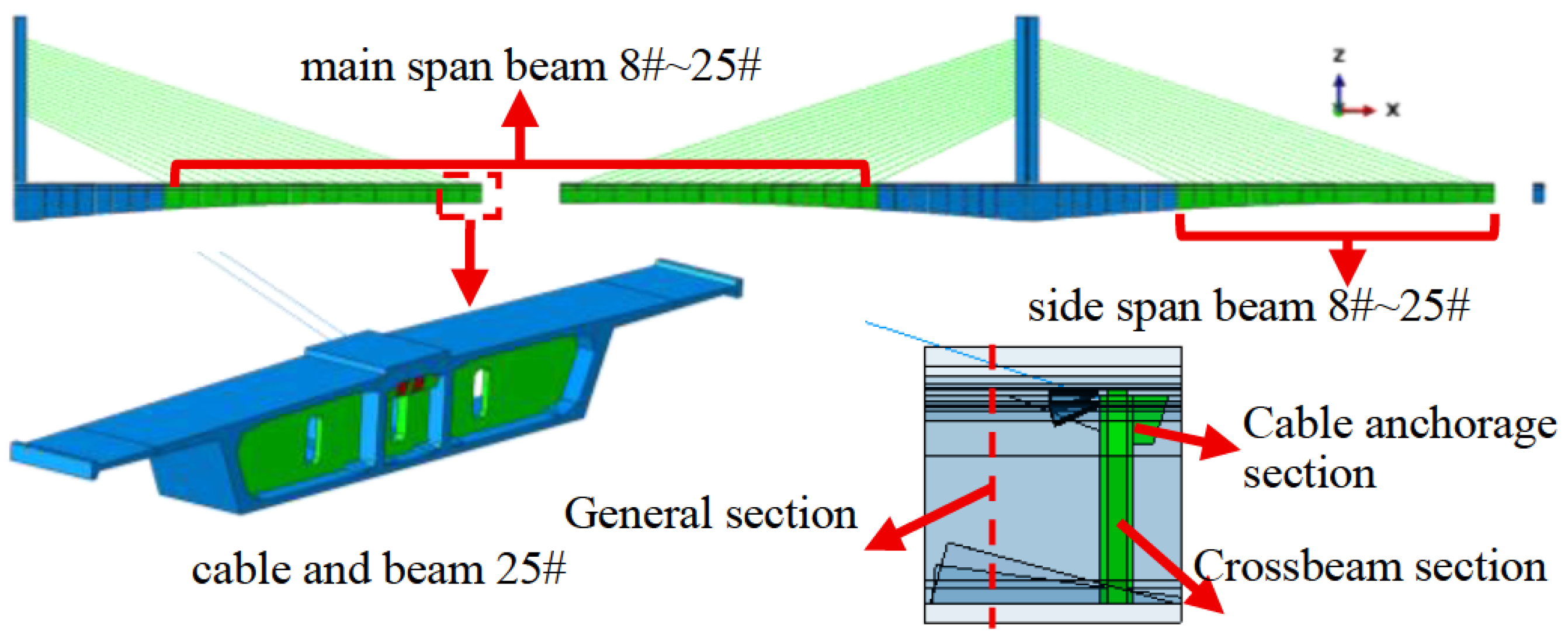
A Python 3.12 preprocessing script imports the beam segments and prestressing tendons into the Abaqus environment. The resulting bridge geometry at a cantilever construction stage is shown in Figure 6.

Due to the complexities of mapped meshing, a free meshing strategy was chosen for the finite element analysis. To address potential accuracy issues with tetrahedral elements in a free mesh, quadratic shape function elements (C3D10) were used. A total of 659,336 quadratic solid elements were produced using the meshing size of 700 mm for the half-bridge model.

Prestressing in the solid elements was simulated by embedding the tendons directly into the solid mesh and applying an initial strain to the tendons. The stay cables were modeled using link elements, with initial tension applied by initial strains.

According to the recommendation in the Abaqus/CAE User’s Guide (2016) [28], the aspect ratio of tetrahedral elements should be controlled below 10. The average aspect ratios obtained from mesh statistics for the present model are as follows: 2.35 for the tower and 2.66 for the main beam. The overall average value for the model is 2.57, which satisfies the recommended standard for mesh quality.

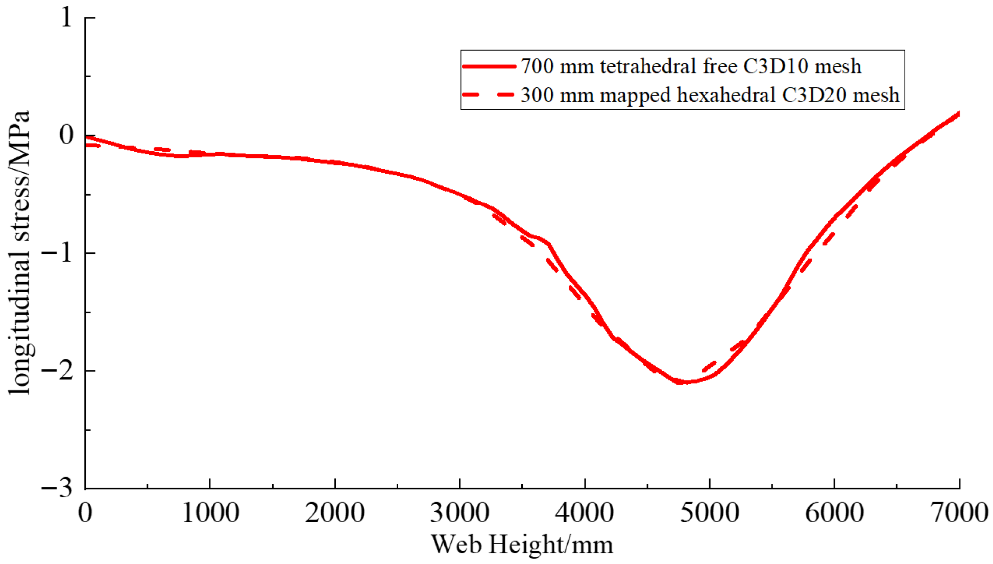
In order to check the accuracy of the free meshing used in the model, two meshing strategies are compared: one using a 300 mm mapped hexahedral C3D20 mesh, and the other using a 700 mm tetrahedral free C3D10 mesh. A cantilever segment was subjected to self-weight and prestress loading (Figure 7), and longitudinal normal stresses were extracted at a path in web as shown in Figure 7. The stress difference between the two meshes was less than 5% (Figure 8). This confirms that the free tetrahedral mesh achieves comparable accuracy to the mapped hexahedral mesh.

3.4. Creep and Shrinkage Models

The evolution of concrete creep and shrinkage models began in the 1970s with a series of models proposed by the European Concrete Committee (CEB) and the International Federation for Prestressing (FIP). This series includes the CEB-FIP (1970), CEB-FIP (1978), and CEB-FIP (1990) models, with the 1990 version [29] also being adopted by Chinese highway bridge design codes [30].

Simultaneously, researchers like Bažant optimized and fitted a large amount of creep test data to propose the simplified and improved B3 model [2]. This was later followed by the more comprehensive B4 model [31], which introduced new constitutive equations and material parameters to more accurately reflect the effects of admixtures and aggregate types.

This paper compares and analyzes the influence of three of these models—CEB-FIP (1990), B3, and B4—on a bridge structure.

(1)

The CEB-FIP (1990) model [29]

The creep coefficient $\phi \left(t,t_0\right)$ given by the CEB-FIP (1990) model is as follows.

$$\phi \left(t,t_0\right)={\phi }_{RH}·\beta \left(f_{cm}\right)·\beta \left(\tau \right){\beta }_c\left(t-t_0\right)$$

(11)

with

$${\phi }_{RH}=1+{\displaystyle \frac{1-RH/{RH}_0}{0.46{\left(h/h_0\right)}^{1/3}}}, \beta \left(f_{cm}\right)={\displaystyle \frac{5.3}{{\left(f_{cm}/f_{cm0}\right)}^{0.5}}}, \beta \left(t_0\right)={\displaystyle \frac{1}{0.1+{\left(t_0\right)}^{0.2}}}, {\beta }_c\left(t-\tau \right)={\left[{\displaystyle \frac{\left(t-t_0\right)}{{\beta }_H+\left(t-t_0\right)}}\right]}^{0.3}$$

(12)

where $h$ denotes the theoretical thickness of the cross-section of the girder dimension in mm, h₀ = 100 mm; $RH$ denotes the annual average ambient humidity (%) and ${RH}_0$ = 100%; $f_{cm}$ denotes the average value of the cube compressive strength for concrete after 28 days of curing and $f_{cm}=$ 10 MPa; $\beta \left(f_{cm}\right)$ reflects the influence of concrete strength on the nominal creep coefficient; ${\beta }_c\left(t-t_0\right)$ describes the development of creep over the duration of loading. In Equation (12), ${\beta }_H$ can be calculated by

$${\beta }_H=150\left[1+{\left(1.2{\displaystyle \frac{RH}{{RH}_0}}\right)}^{18}\right]{\displaystyle \frac{h}{h_0}}+250$$

(13)

where $h_0$ = 100 mm.

The concrete shrinkage strain ${\epsilon }_{sh}\left(t\right)$ of the CEB-FIP (1990) model is as follows.

$${\epsilon }_{sh}\left(t\right)={\epsilon }_s\left(f_{cm}\right){\beta }_{RH}{\beta }_s\left(t-t_s\right)$$

(14)

With

$$\begin{gathered} {\epsilon }_s\left(f_{cm}\right)=\left[160+10{·\left(9-f_{cm}/f_{cm\mathrm{o}}\right)\beta }_{sc}\right]·{10}^{-6},{\beta }_{RH}=1.55\left[1-{\left(RH/{RH}_0\right)}^3\right] \\ {\beta }_s\left(t-t_s\right)={\left[{\displaystyle \frac{\left(t-t_s\right)}{350{\left(h/h_0\right)}^2+\left(t-t_s\right)}}\right]}^{0.5} \end{gathered}$$

(15)

where $t_s$ denotes the concrete age at the start of shrinkage, assumed to be 3 days; the value of ${\beta }_{sc}$ depends on the cement type, and ${\beta }_{sc}$ = 5.0 for ordinary Portland cement; ${\epsilon }_s\left(f_{cm}\right)$ reflects the influence of concrete strength on the nominal shrinkage coefficient.

It should be noted that the influence of member geometry and ambient relative humidity has already been incorporated in the adopted creep and shrinkage formulations. The parameter h in Equations (11)–(15) represents the theoretical thickness of the cross-section, which effectively reflects the influence of the box-girder dimensions on moisture diffusion and time-dependent deformation. Therefore, the geometric effect is implicitly included in the calculation of the creep and shrinkage coefficients.

In this study, the annual average relative humidity was taken as 70%, in accordance with the bridge design documents and the design code [30]. This value reflects the actual site condition and is relatively stable during the bridge’s service period.

(2)

B3 and B4 Model [2,31]

The CEB-FIP (1990) is an empirical, regression-based model with parameters derived from statistical fits of experimental data. This approach limits their adaptability to evolving concrete compositions, such as those with new admixtures, and to non-standard environmental conditions.

To overcome these limitations, Bažant developed a model system based on the physical mechanisms of creep. This approach separates the total creep strain into two independent components: basic creep and drying creep. This framework led to the development of the more theoretically robust B3 model [2].

The B4 model [31] was subsequently developed as an advancement of the B3 model. This model quantitatively describes the combined impact of aggregate type, mineral admixtures, and chemical admixtures on the creep process by introducing new parametric equations, including a correction factor for the aggregate’s modulus of elasticity and a reaction activity coefficient for admixtures.

Due to the complexity of the B3 and B4 models and the large number of parameters involved, their full equations and detailed parameters are provided in Appendix A for brevity.

3.5. Comparison of Creep and Shrinkage Models

Based on the parameters defined above, the evolution of the creep coefficients and shrinkage strains over time of the four creep models was obtained. The comparative results are shown in Figure 9. In producing Figure 9, the theoretical thickness of the member h is taken as 1000 mm.

As shown in Figure 9a, all models exhibit a non-linear, monotonically increasing creep coefficient, with a logarithmic evolution that reflects the decaying creep rate of viscoelastic materials. The B-series models show a significantly higher creep coefficient than the CEB model. The B4 model, which includes a correction factor for admixtures and fly ash, has a growth trend similar to the B3 model but with smaller values.

The CEB, B3, and B4 models all show a consistent growth trend in their absolute shrinkage strain values, with the rate decreasing over time. The CEB model has the lowest shrinkage strain and a slower growth rate. In contrast, the B4 model has a larger value and a more significant long-term growth trend than the B3 model.

Concrete creep and shrinkage are complex processes influenced by multiple factors, including material type, manufacturing, and environmental conditions. This introduces considerable uncertainty into their prediction.

Table 4. Coefficients of variation (C.o.V.) for creep and shrinkage [33].

Model	Creep Coefficient of Variation	Shrinkage Coefficient of Variation
CEB	0.470	0.415
B3	0.366	0.410
B4	0.273	0.316

provides the coefficient of variation for each creep and shrinkage prediction model, based on values from reference [32]. These coefficients of variation will be used in the probabilistic analysis in Section 5 and Section 6.

The C.o.V. values in Table 4 represent the statistical deviation between the predicted and measured results obtained from large experimental databases and reflect the overall quality of fit of models. Consequently, the C.o.V. does not include the explained variability caused by known influencing factors such as geometry, humidity, or concrete strength, since these are explicitly accounted for in the predictive formulations. All uncertainties were treated as time-invariant constants, consistent with the probabilistic model in reference [32].

In Table 4, models B3 and B4 exhibit smaller variability in their shrinkage and creep predictions than the CEB-FIP90 model. This lower uncertainty is because they incorporate the physical mechanisms of shrinkage and creep and account for specific concrete mix proportions. The B4 model has the least variability, as it also considers the effects of aggregate and admixtures.

3.6. Implementation of Creep and Shrinkage in Solid Element Analysis

Standard solid element analysis software usually does not have the built-in capability to simulate concrete shrinkage and creep. This section presents a three-dimensional constitutive model for these effects, as originally described in [33]. This model will be implemented in solid element analysis using the Abaqus commercial software through self-developed material subroutines.

Since the analysis incorporates time-dependent creep and shrinkage, material nonlinearity was included. The built-in Newton–Raphson iterative scheme in Abaqus was used, with a convergence tolerance of 0.5% on the displacement residual and a maximum of 20 iterations per increment.

It is well-known that the total strain $\left\{\epsilon \left(t\right)\right\}$ and any time t can be divided into elastic strain $\left\{{\epsilon }^e\left(t\right)\right\}$, creep strain $\left\{{\epsilon }^c\left(t\right)\right\}$ and shrinkage strain $\left\{{\epsilon }_{sh}\left(t\right)\right\}$ as shown in Equation (1).

$$\left\{\epsilon \left(t\right)\right\}=\left\{{\epsilon }^e\left(t\right)\right\}+\left\{{\epsilon }^c\left(t\right)\right\}+\left\{{\epsilon }_{sh}\left(t\right)\right\}$$

(16)

In Equation (17), the strain tensor in 3D space is written into vector $\left\{\epsilon \right\}={\left[{\epsilon }_x,{\epsilon }_y,{\epsilon }_z,{\gamma }_{xy},{\gamma }_{yz},{\gamma }_{zx}\right]}^T$, where ${\epsilon }_x,{\epsilon }_y,{\epsilon }_z$ represent normal strain and ${\gamma }_{xy},{\gamma }_{yz},{\gamma }_{zx}$ represent shear strain, respectively.

The elastic strain when the modulus of elasticity E(t) dependance on time t is considered can be written as:

$$\left\{{\epsilon }^e\left(t\right)\right\}=\left[\begin{array}{c}A\end{array}\right]{\displaystyle \frac{\left\{\Delta {\sigma }_0\right\}}{E_{\left(t0\right)}}}+{\int }_{t_0}^t{\displaystyle \frac{1}{E_{\left(\tau \right)}}}\left[A\right]\left\{{\displaystyle \frac{\mathrm{d}\sigma \left(\tau \right)}{\mathrm{d}\tau }}\right\}\mathrm{d}\tau$$

(17)

where $\left\{\Delta {\sigma }_0\right\}$ denotes the stress increment for the initial loading at time $t0$, $\tau$ is the intermediate loading time which causes a stress incremental $\mathrm{d}\sigma \left(\tau \right)$, and $\left[A\right]$ considers the Poisson’s ratio $\mu$ when relating strain and stress vector besides the modulus of elasticity in 3D space.

$$\left[\begin{array}{c}A\end{array}\right]=\left[\begin{array}{ccccccc}1& -\mu & -\mu & 0& 0& 0& \\ & 1& -\mu & 0& 0& 0& \\ & & 1& 0& 0& 0& \\ & & & 2\left(1+\mu \right)& 0& 0& \\ & & & & 2\left(1+\mu \right)& 0& \\ & & & & & 2\left(1+\mu \right)& \end{array}\right]$$

(18)

Based on linear creepage theory, the creep strain can be linearly sum up for incremental at different loading time by

$$\left\{{\epsilon }^c\left(t\right)\right\}=\left[\begin{array}{c}A\end{array}\right]\left\{\Delta {\sigma }_0\right\}C\left(t,t0\right)+{\int }_{t_0}^{t}C\left(t,\tau \right)\left[A\right]\left\{{\displaystyle \frac{\mathrm{d}\sigma \left(\tau \right)}{\mathrm{d}\tau }}\right\}$$

(19)

where $C\left(t,\tau \right)$ represents the creep compliance function, represents the creep strain at time t when loaded by unit stress at time $\tau$. It is related to the creep coefficient by $C\left(t,\tau \right)=\phi \left(t,\tau \right)/E\left(\tau \right)$ with $E\left(\tau \right)=E_{28}{\mathrm{e}}^{0.25(1-{\left({\displaystyle \frac{28}{\tau }}\right)}^{0.5})}$ is the Young’s modulus dependent on the loading age $\tau$. $E_{28}$ mean Young’s modulus at 28 days.

The creep compliance function can be fitted into the following Dirichlet series to avoid storing creep strain history during numerical calculations [33].

$$C\left(t,\tau \right)={\sum }_{j=1}^m{\varphi }_j\left(\tau \right)\left[1-{\mathrm{e}}^{-r_j\left(t-\tau \right)}\right]$$

(20)

The fitted coefficient ${\varphi }_j\left(\tau \right)$ and $r_j$ for the CEB-FIB creep coefficient are shown in Appendix B as an example. In Equation (20), the parameter m = 4 was used for the Dirichlet series expansion, which provides sufficient accuracy as shown in Appendix B.

Equations (16) and (17) should be cast into an incremental format to facilitate the nonlinear analysis due to the creep-induced nonlinear material. For the n-th time step from $t_{n-1}$ to $t_n$. Based on Equation (16), the strain incremental is

$$\left\{∆{\epsilon }_n\right\}=\left\{∆{\epsilon }_n^e\right\}+\left\{∆{\epsilon }_n^c\right\}+\left\{∆{\epsilon }_n^{sh}\right\}$$

(21)

From Equation (17), the elastic strain increment is

$$\left\{\Delta {\epsilon }_n^e\right\}=\left[A\right]\left\{\Delta {\sigma }_n\right\}/E\left(t_{n-0.5}\right)$$

(22)

where $E\left(t_{n-0.5}\right)$ denotes the average modulus of elasticity during time increment from $t_{n-1}$ to $t_n$. The time-dependent modulus of elasticity based on the Chinese design code [30] is also shown in Appendix A.

Based on Equations (19) and (20), the creep strain increments can be obtained through the following recursive manner.

$$\left\{\Delta {\epsilon }_n^c\right\}=\left\{{\eta }_n\right\}+q_n\left[A\right]\left\{\Delta {\sigma }_n\right\}$$

(23)

$$q_n=C\left(t_n,t_{n-0.5}\right)={\sum }_{j=1}^m{\varphi }_j\left(t_{n-0.5}\right)\left[1-{\mathrm{e}}^{-r_{j}0.5\Delta t_n}\right]$$

(24)

$$\left\{{\eta }_n\right\}={\sum }_{j=1}^m\left(1-{\mathrm{e}}^{-r_j{\Delta \mathrm{t}}_n}\right)\left\{{\omega }_{j,n}\right\}$$

(25)

$$\left\{{\omega }_{j_{,n}}\right\}=\left\{{\omega }_{j,n-1}\right\}{\mathrm{e}}^{-r_j\Delta t_{n-1}}+\left[A\right]\left\{\Delta {\sigma }_{n-1}\right\}{\varphi }_j\left(t_{n-1-0.5}\right){\mathrm{e}}^{-0.5r_j\Delta t_{n-1}}$$

(26)

with the initial value $\left\{{\omega }_{j,1}\right\}=\left[A\right]\left\{\Delta {\sigma }_0\right\}{\varphi }_j\left(t_0\right)$ for recursive calculation. It should be noted that the intermediate vectors in Equations (23)–(26) all have six elements as they are related to the stress vector $\left\{\Delta \sigma \right\}$.

By substituting Equations (21) and (22), the elastic stress increment can be written as

$$\left\{\Delta {\sigma }_n\right\}=\left[A\right]/E\left(t_{n-0.5}\right)\left(\left\{∆{\epsilon }_n\right\}-\left\{∆{\epsilon }_n^c\}-\left\{∆{\epsilon }_{sh}\right\}\right\}\right)$$

(27)

By solving $\Delta {\sigma }_n$ from Equations (23)–(27), the elastic stress increment $\left\{\Delta {\sigma }_n\right\}$ can be obtained.

$$\left\{\Delta {\sigma }_n\right\}={\left[A\right]}^{-1}/(1/E(t_{n-0.5})+q_n)\left(\left\{∆{\epsilon }_n\right\}-\left\{{\eta }_n\right\}-\left\{∆{\epsilon }_{sh}\right\}\right)$$

(28)

Equations (25), (26) and (28) are programmed into the UMAT routine to define the relation between the strain increment $\left\{∆{\epsilon }_n\right\}$ and $\left\{\Delta {\sigma }_n\right\}$ increment. The vector $\left\{{\eta }_n\right\}$ required in Equation (25) can be obtained based on the known vectors $\left\{\Delta {\sigma }_{n-1}\right\}$, $\left\{{\omega }_{j,n-1}\right\}$ of the previous time step. In Equation (28) the shrinkage strain increment $∆{\epsilon }_{sh}$ can be obtained using the shrinkage models.

Some studies [33] only present Equations (16)–(26). However, it is important to note that establishing the constitutive relationship (Equation (28)) between the elastic stress increment $\left\{\Delta {\sigma }_n\right\}$ and the total strain increment $\left\{∆{\epsilon }_n\right\}$ at the current time step is crucial. The concrete constitutive model should be programmed based on this relationship.

4. Deterministic Analysis: Discrepancies Between Solid and Beam Element Models

Unexpected cracking and long-term deflection in extradosed bridges often stem from the inadequacy of beam theory in standard design practice. For complex structures like cantilever-constructed box girders, much of the girder acts as a disturbed region due to tendon anchorage, where the linear strain distribution assumed by beam theory is invalid. Beam analysis fails to capture the true stress distribution and cannot account for critical effects like shear lag.

In this section, we apply the models from Section 3 to compare beam and solid element models, focusing on long-term deformation, their sensitivity to creep and shrinkage parameters, and structural stress.

4.1. Long-Term Deformation

Figure 10 compares the mean value of the long-term deflection at mid-span, as obtained from solid and beam element models, using the CEB-FIP90 model. It shows that the long-term deflection predicted by the solid element model is significantly greater than that predicted by the beam model. Twenty years after the bridge’s completion, the beam element analysis underestimates the long-term deflection by approximately 14% (105.9 mm vs. 93.1 mm).

The long-term deflection results presented in Figure 10 include both the creep and shrinkage effects of concrete as modeled in Section 3.4. The influences of temperature variation and tendon relaxation were not considered in the present computations. Although tendon relaxation can lead to additional deflection in actual bridges, its variability is relatively small and well defined. This study therefore focuses on the uncertainty associated with creep and shrinkage, which represent the primary sources of long-term deformation variability in concrete structures.

4.2. Sensitivity of Long-Term Deformation to Creep and Shrinkage Parameters

The bridge’s response sensitivity to the Creep and Shrinkage Parameters can be calculated according to Equation (8). Firstly, the mean response of the structure $g\left({\mu }_{\mathrm{X}1},{\mu }_{\mathrm{X}2},\dots ,{\mu }_{Xs}\right)$ is obtained using the mean values of creep and shrinkage parameters for the bridge models in Section 3.2 and Section 3.3. Secondly, vary the shrinkage and creep parameters by one standard deviation, respectively, and use the modified parameter to re-analysis the structure to get $g\left({\mu }_{\mathrm{X}1},{\mu }_{\mathrm{X}2},\dots ,{\mu }_{\mathrm{X}\mathrm{i}}+{∆}_i\dots ,{\mu }_{Xs}\right)$. Finally, use Equation (8) to calculate the sensitivity coefficients $a_i$ of the bridge’s long-term deflection to the creep and shrinkage parameters. The comparison between the solid and beam models is presented in

Table 5. Sensitivity Coefficients of the 20-Year Long-Term Deflection $a_i^{\ast }$.

Random Variable	BEAM Element Analysis	SOLID Element Analysis	Solid/Beam Ratio
Creep Coefficient	−0.281	−0.376	1.340
Shrinkage Coefficient	−0.173	−0.250	1.444

, using the CEB-FIP90 model for the calculations.

As can be seen in Table 5, the sensitivity coefficients of the solid element model are approximately 34% to 44% larger than those of the beam model. This is likely to occur because the beam element’s plane section assumption imposes additional constraints, artificially increasing the bridge’s rigidity and underestimating the sensitivity coefficients. Therefore, when considering the uncertain effects of creep and shrinkage, using a beam element model will significantly underestimate the uncertainty of the bridge’s long-term deformation.

4.3. Comparison of Girder Stress from the Beam and Solid Element Analysis

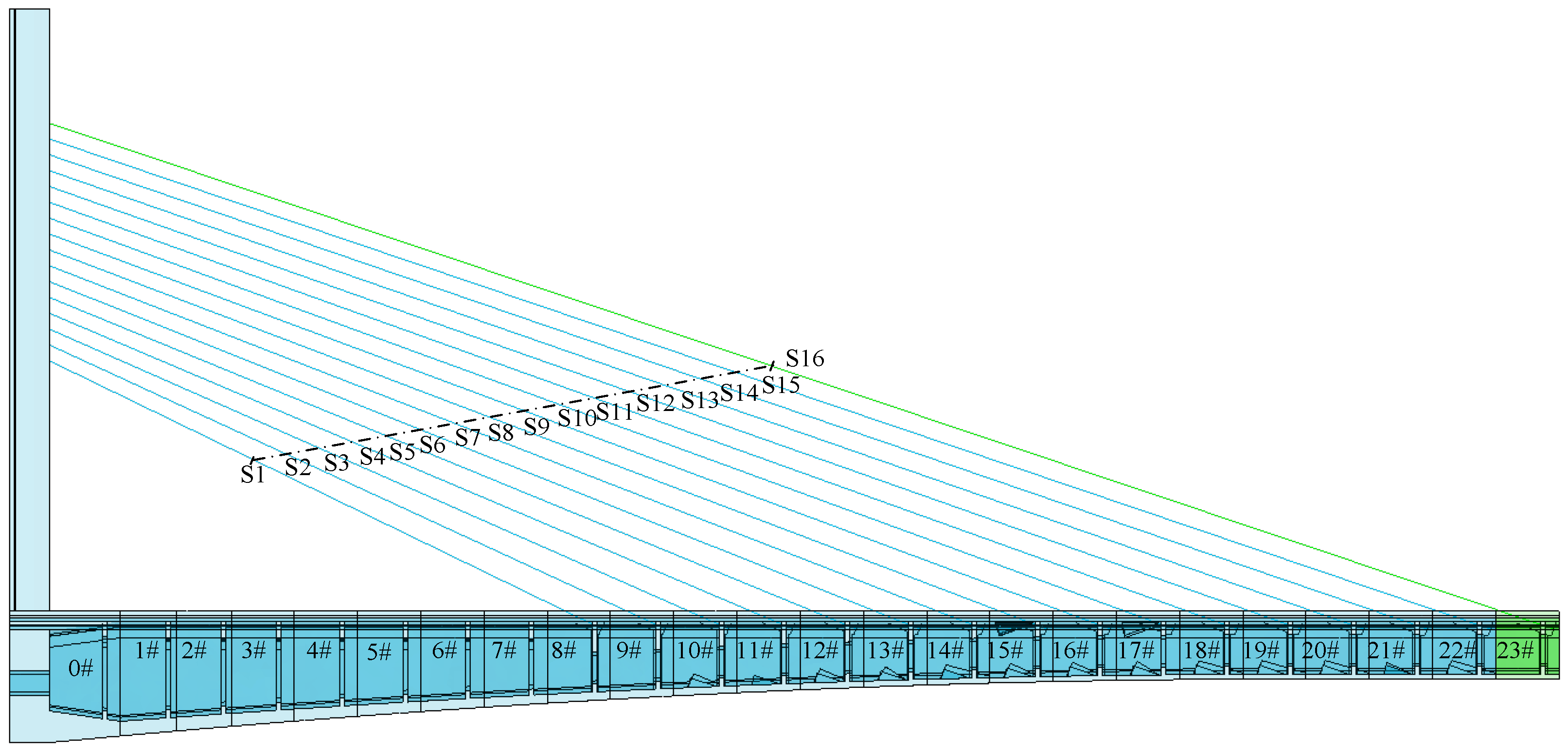
The stress in a cable-supported segment during the construction stage after tensioning stay cable S16 (the third cable from the end; see Figure 11) along the path shown in Figure 12 is analyzed in this part. This construction stage is close to the maximum cantilever state, where the horizontal component of the cable force is the largest.

To analyze the influence of the stay cable on web stress, Figure 13 compares the stresses after cable tensioning with results from the beam analysis according the Chinese design code [30].

As Figure 13a shows, the solid element analysis produces a non-linear distribution of longitudinal normal stress along the girder depth, clearly diverges from the beam analysis. Near the top boss, the solid element predicts smaller compression stress than the beam analysis, this may be due to the anchorage block share some cable forces, which is not accounted by the beam element.

The shear stress from the solid element model (red line) differs significantly from the beam element model (blue line) in Figure 13b. The shear stress direction is opposite in most of the web. The solid model’s vertical shear stress shows a sharp change near the anchorage point, increasing to 0.78 MPa on the top slab boss.

Figure 13c shows that the vertical normal stress in the web is primarily induced by vertical prestressing. The beam element analysis overestimates this pre-compressive stress. The tensile stress in Figure 13d from solid element differs from the beam element analysis about 1.5–2.0 MPa across the cross section. Considering the stress limit is only 2.68 MPa, this discrepancy is not acceptable in cracking evaluation for prestressing concrete bridges. Therefore, the tensile stress evaluation should be based on the solid element analysis.

5. Comparison of Probabilistic Analysis Methods

Due to the high computational cost of the solid element models, with a single analysis taking over 15 h (compared with 20 min using the beam analysis), using sampling-based probabilistic methods is computationally impractical. Therefore, this section employs the more efficient beam element model to first compare the accuracy of the First-Order Second-Moment (FOSM) method against the quasi-Monte Carlo sampling method. This comparison serves to validate the FOSM method’s accuracy in a controlled environment before applying it to the computationally demanding, high-fidelity solid element analysis in the subsequent sections. To thoroughly test the methods’ adaptability to multiple variables, six random structural parameters were considered. The probabilistic characteristics of these parameters are detailed in

Table 6. Probabilistic characteristics of the Random Variables.

Random Variable	Probability Distribution	Mean	Coefficient of Variation
Concrete Density $\rho$ [34]	Normal	25 kN/m3	0.03
Concrete Elastic Modulus E [35]	Normal	35,500 MPa	0.04
Tendon Stress $F$ [36]	Normal	1395/1300 MPa	0.088
Cable Stress $F_{con}$ [36]	Normal	Design Value	0.06
Creep Coefficient φ [32]	Normal	1.85	0.470
Shrinkage Coefficient ${\epsilon }_{sh}$ [32]	Normal	3.36 × 10−4	0.415

.

We used the sampling method based on number theory, as described in Section 2.1, to discretize the space of the random variables. For the six random variables in question, an initial set of 2129 uniformly distributed sample points was generated within the unit hypercube [0, 1]⁶ using the parameters n = 2129, h₁ = 1, h₂ = 41, h₃ = 1681, h₄ = 793, h₅ = 578, and h₆ = 279, as specified in reference [25].

In the probabilistic analysis, all random variables were initially assumed to follow normal distributions for consistency with the First-Order Second-Moment (FOSM) method. Although the creep coefficient is a positive-valued parameter, the normal distribution has been widely used in previous probabilistic studies of time-dependent effects in concrete structures [37,38], owing to its analytical simplicity and direct compatibility with the FOSM formulation.

To optimize computational efficiency for a multi-dimensional Gaussian space, this initial set was refined. We leveraged the property that the joint probability density is very low near the boundaries of the distribution. Accordingly, we filtered the initial set by selecting only the sample points located inside a hypersphere of radius r = 0.5 using Equation (3). This screening process reduced the number of samples to 166 by excluding the low-probability points in the tail regions of the distribution. The sum of the probabilities of the retained 166 samples is 97.65%, making the set highly representative and ensuring that the statistical outcomes are not compromised. This sample size is considered sufficient for convergence, as demonstrated in other studies where a similar number of samples proved effective for problems with an even greater number of variables [33].

To ensure physical realism, a truncated normal distribution was implemented to exclude negative samples. In the quasi-Monte Carlo sampling with 166 points, only 5 samples were negative. These negative samples were discarded, and their probability weights were redistributed to the remaining points.

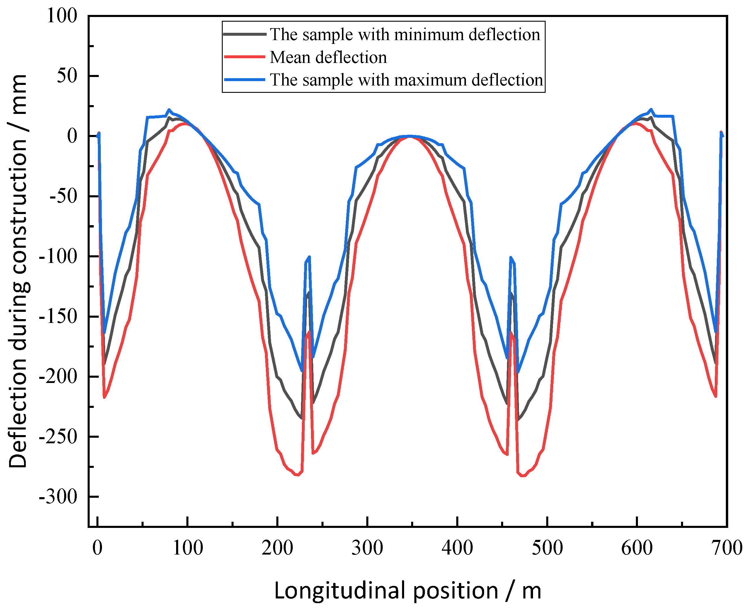
This section examines the cumulative deformation of the bridge during construction in order to test the practicality of the First-Order Second-Moment (FOSM) method in complex conditions such as staged construction and time-dependent effects. The CEB-FIB90 model was employed to model creep and shrinkage. The 161 creep and shrinkage parameter sets were imported into the beam element model to simulate the construction process and calculate the girder’s deflection during construction. Figure 14 shows that, at the completion stage, the difference between the maximum and minimum mid-span deflection samples exceeds 80 mm.

The local discontinuities observed in Figure 14 around 250 m and 450 m correspond to the ends of the two main cantilever arms, which are the closure segment locations. In the cantilever construction simulation, each newly installed segment is initially activated at its design elevation. Because deflection develops only under the self-weight of subsequently added segments, the front-end nodes of the last installed cantilever segments remain nearly at their original elevation until the deck pavement (secondary dead load) is applied. This modeling feature leads to the small step-like discontinuities visible in the deflection profile.

The FOSM method involves calculating the sensitivity coefficients of the structural response to random parameters. For each of the six random variables, one additional structural analysis must be performed by varying this variable at least once. To verify the accuracy of the first-order linear expansion in Equation (6), four structural analyses were performed for each random variable at four different values (${\mu }_{\mathrm{X}\mathrm{i}}-2{\delta }_{Xi}$, ${\mu }_{\mathrm{X}\mathrm{i}}-{\delta }_{Xi}$, ${\mu }_{\mathrm{X}\mathrm{i}}+2{\delta }_{Xi}$, ${\mu }_{\mathrm{X}\mathrm{i}}+{\delta }_{Xi}$) as shown in Figure 15. The mid-span deflection showed a nearly linear relationship with respect to each random variable, consistent with the FOSM method’s assumptions.

Based on this data, we calculated the sensitivity coefficients for the bridge’s mid-span construction deflection using Equation (8), and these are shown in

Table 7. Sensitivity coefficient of bridge deflection during construction based on the beam analysis.

Random Variable	${\mathit{a}}_{\mathit{i}}^{\mathit{*}}$ (mm)	Random Variable	${\mathit{a}}_{\mathit{i}}^{\mathit{*}}$ (mm)
Concrete Density	−7.57	Cable stress	2.3
Concrete Elastic Modulus	2.9	Creep Coefficient	−12.84
Tendon stress	6.8	Shrinkage Coefficient	0.33

. The table shows that the mid-span deflection during construction is most sensitive to the creep coefficient, followed by concrete self-weight and tendon prestressing.

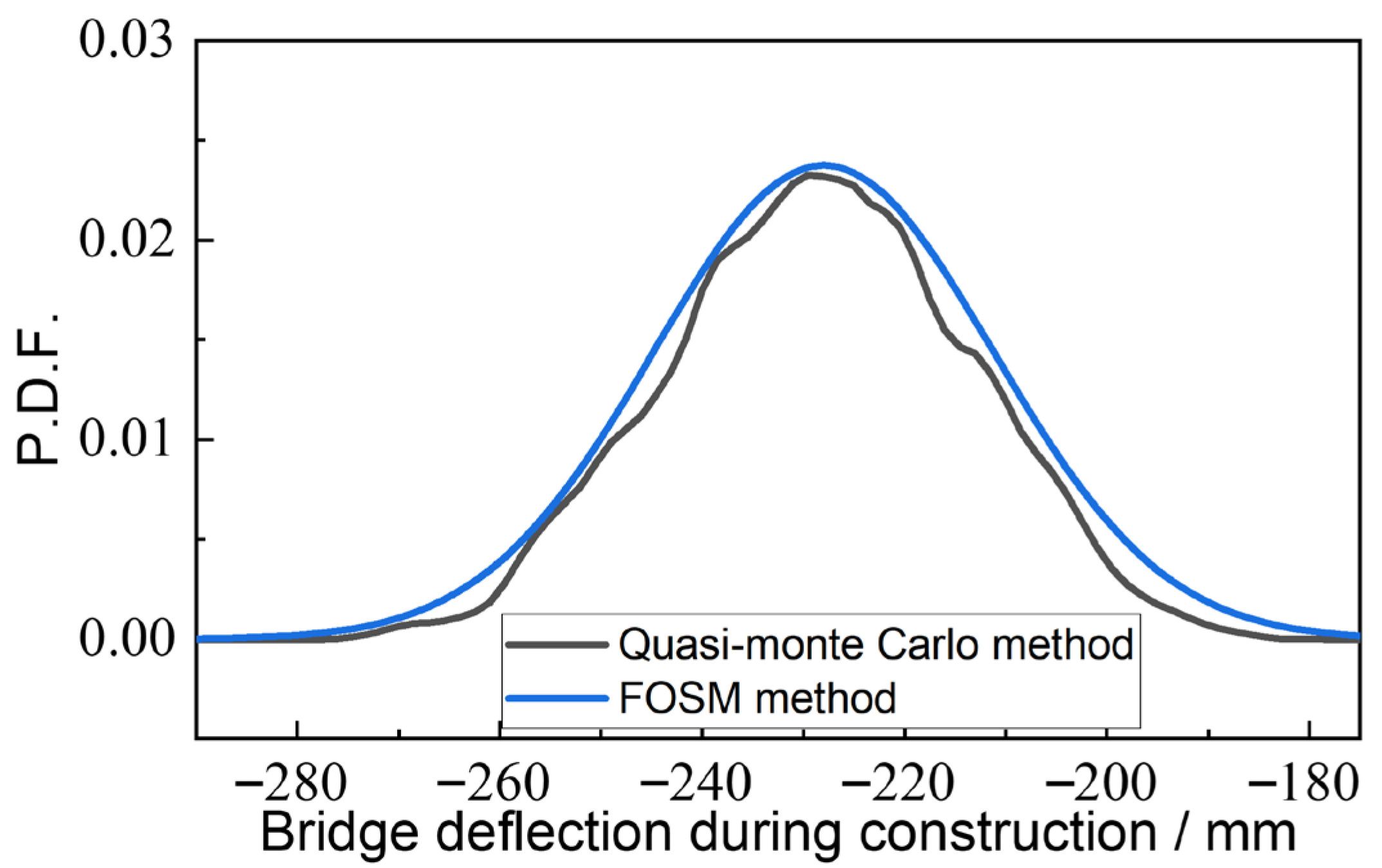
The First-Order Second-Moment (FOSM) method yielded a mean of −229.69 mm and a standard deviation of 16.80 mm for the maximum deflection at the completion stage using Equations (9) and (10). The mean and standard deviation errors between the two methods were 2.63% and 6.33%, respectively.

Figure 16 shows the probability density of the bridge’s deflection during construction as determined by two probabilistic analysis methods. The probability density for the sampling method was numerically solved from the samples using the probability density evolution equation [6]. The probability density for the First-Order Second-Moment (FOSM) method was plotted based on a normal distribution derived from its mean and standard deviation. As Figure 16 shows, the probability densities from the two methods fit well, indicating that the FOSM method has sufficient accuracy. The FOSM method required only seven model analyses (one for the mean response and one for each of the six random variables), which is just 4.3% of the 161 analyses needed for the Quasi-Monte Carlo sampling method.

6. Probabilistic Analysis of Long-Term Deformation with the Solid Element Model

The deterministic analyses in Section 4 have shown that the mean values of bridge deformation and stress predicted by the beam and solid element models differ considerably. The solid element model yields approximately 14% larger long-term deflection and up to 2 MPa higher principal tensile stress in critical regions. Because the 95% confidence interval in the probabilistic analysis is determined by both the mean and the standard deviation, and the mean component contributes more significantly to the total response, these differences indicate that the probabilistic outcomes of the two models would also differ substantially.

Hence, it is unnecessary to repeat the probabilistic analysis using beam elements. Beam-based probabilistic studies of creep and shrinkage have already been widely reported in the literature [19,20,21]. The focus of the present work is therefore to demonstrate a feasible solid-element-based probabilistic framework for evaluating long-term uncertainty in complex bridges, overcoming the computational limitations that have previously hindered such analyses.

A single solid element analysis of the bridge in this study takes over 15 h, rendering sampling-based probabilistic analysis methods computationally impractical. The previous section demonstrated the accuracy of the first-order second-moment (FOSM) method for beam element analysis. Since probabilistic analysis methods are independent of the structural analysis method, it can be assumed that the FOSM method is also sufficiently accurate for analyzing bridge deformation using solid elements.

It is important to note that the construction-period deflection analyzed in the previous section is used to set the pre-camber and can theoretically be largely eliminated through precise construction control and parameter identification. This section, however, analyses the long-term deflection after construction, relating to the bridge’s long-term operational performance. Many prestressed continuous girder bridges have exhibited unexpectedly large long-term deflections, potentially due to deficiencies in the analysis method, including: (1) beam models failing to accurately reflect structural stiffness; (2) uncertainty in actual creep and shrinkage parameters; (3) code-prescribed creep and shrinkage parameters being based on short-term test data, which is insufficient for predicting long-term deformation. Therefore, this section uses a solid element model and considers the uncertainty of creep and shrinkage parameters and compares the CEB-FIP90, B3, and B4 models on long-term deflection estimation.

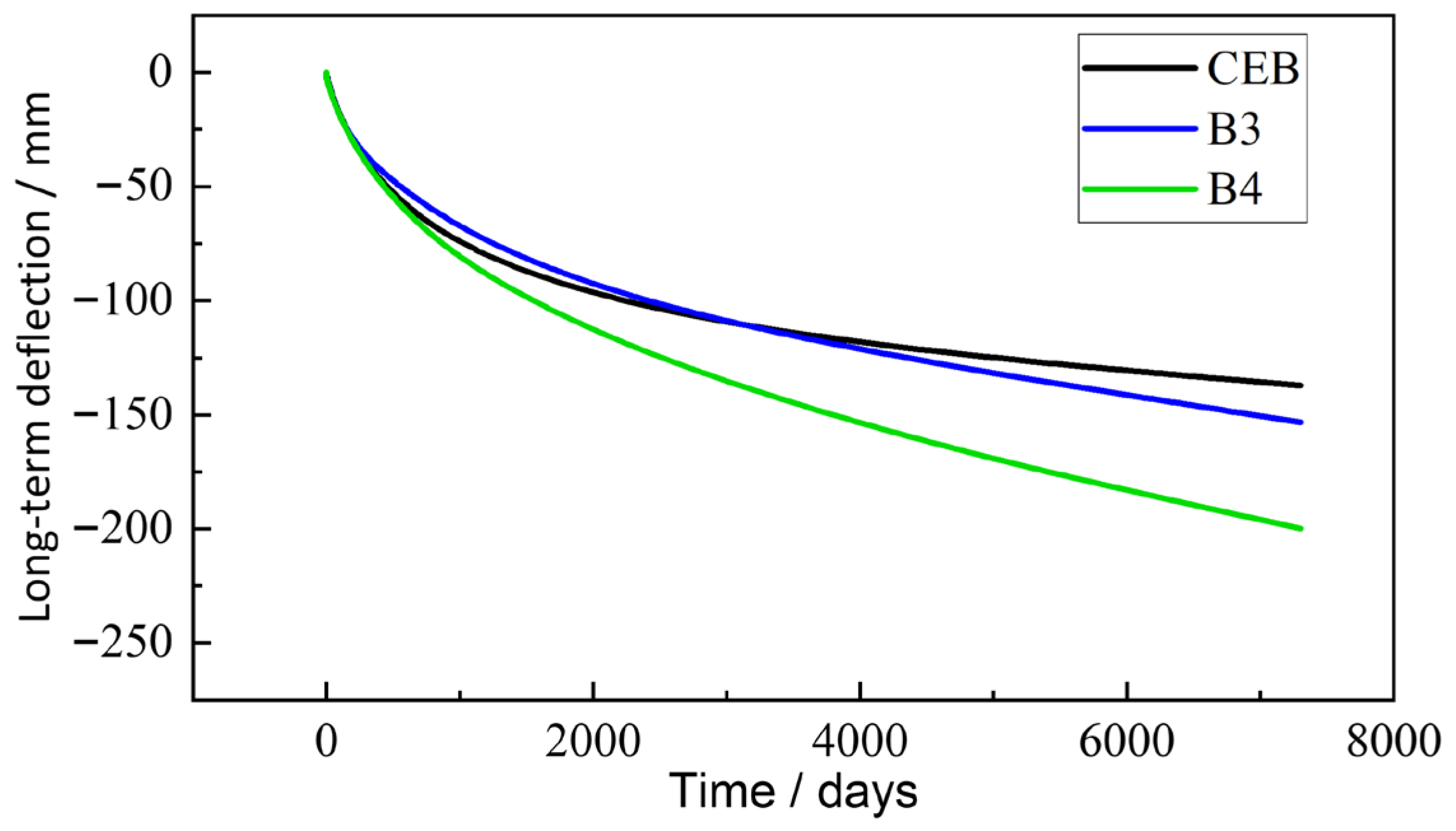
By using the creep and shrinkage models and their parameters from Section 3.4 for a solid element analysis, the mean values of the long-term deflection at the mid-span of the bridge can be obtained as shown in Figure 17. Figure 17 shows that the mean value of the long-term deformation obtained from the B3 and B4 models is greater than that obtained from the CEB model. This is primarily because the experimental data used to fit the CEB model typically covers a period of no more than 20 years, resulting in less conservative (i.e., smaller) prediction for ultra-long-term deflection. Conversely, the B3 and B4 models demonstrate superior performance in long-term time extrapolation by incorporating the physical mechanisms of creep and shrinkage. The B4 model predicts a long-term deflection 30% greater than the B3 model. This is because the B4 model considers factors such as cement type and admixtures, and includes independent autogenous shrinkage as well as drying shrinkage (see Appendix A, Equation (A26)). This results in a larger shrinkage coefficient (see Figure 9).

Table 8. Statistics of long-term deflection at 20 years from bridge completion based on solid element analysis.

Creep-Shrinkage Model	Coefficient of Variation for Parameters		Long-Term Deflection Sensitivity Coefficient (mm)		Statistical Values of Long-Term Deflection (mm)
	Creep	Shrinkage	Creep	Shrinkage	Mean Value	Standard Deviation	95% Confidence Value
CEB	0.47	0.415	−39.86	−26.47	−137.19	49.16	−218.058
B3	0.366	0.41	−35.59	−14.72	−149.6	40.2	−215.729
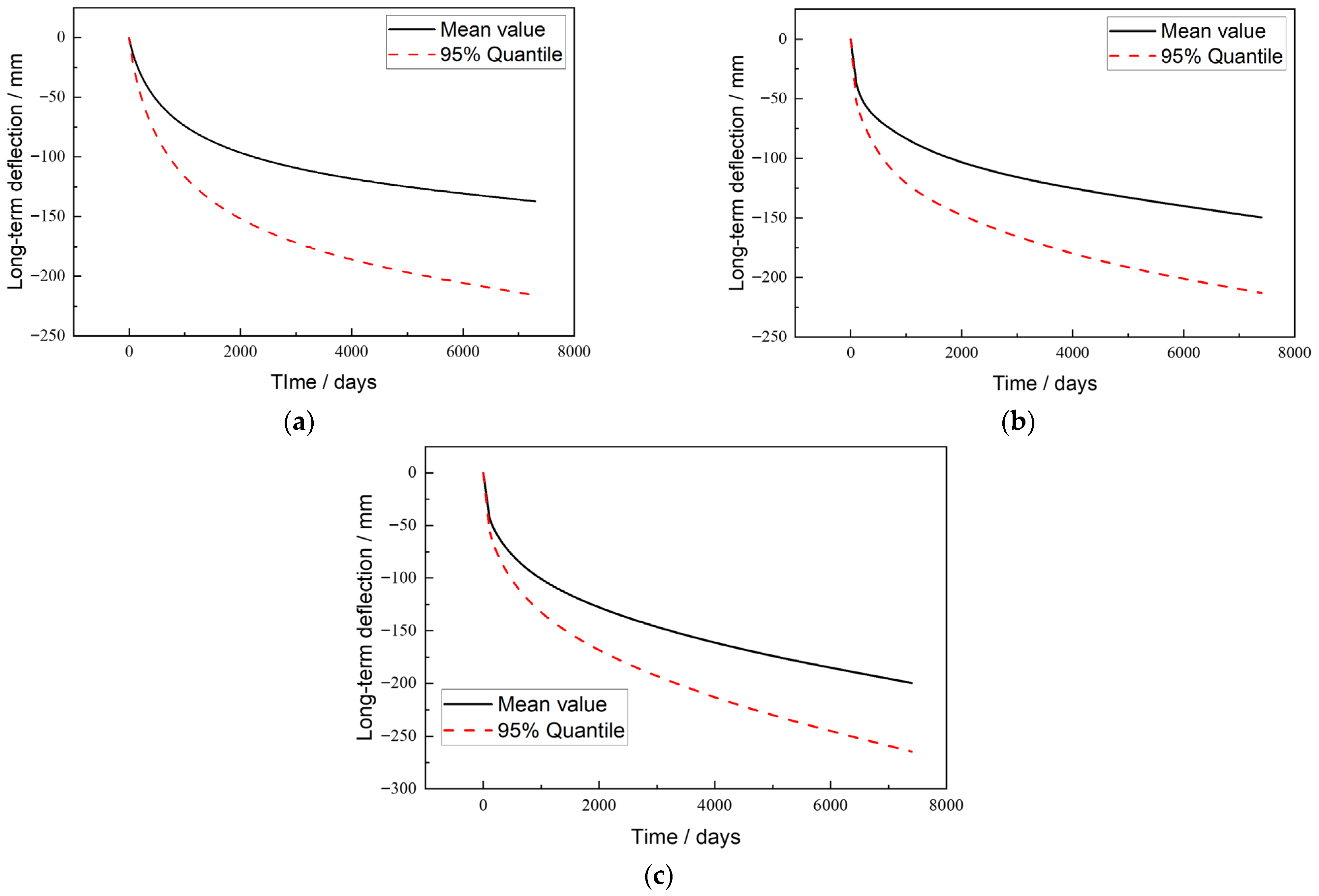
B4	0.273	0.316	−30.88	−24.62	−199.62	41.14	−267.295

shows the results of the probabilistic analysis of the bridge’s long-term deflection, as calculated using the First-Order Second-Moment (FOSM) method. The FOSM analysis procedure involves carrying out two additional structural analyses by altering the creep and shrinkage parameters by one standard deviation, respectively. These results are then used in Equation (8) to obtain the sensitivity coefficients and Equations (9) and (10) are used to calculate the standard deviation of the response. Finally, the long-term downward deflection at the 95% confidence level is determined from the standard deviation, assuming a normal distribution.

As can be seen from Table 8, the long-term deflection of the bridge is more sensitive to creep than to shrinkage. Furthermore, the CEB model shows higher sensitivity than the B3/B4 models. The B4 model’s higher shrinkage sensitivity coefficient compared to the B3 model is likely due to the increased shrinkage deformation caused by the inclusion of autogenous shrinkage.

Table 8 also shows that the standard deviations for long-term deflection are fairly consistent across the three models. The standard deviation of bridge deflection for the CEB model is approximately 25% larger than those for the B3 and B4 models. This difference arises because the CEB model is based solely on a statistical relationship, whereas the B3 and B4 models incorporate more physical parameters, thereby reducing model uncertainty. The table shows differences of up to 24% in maximum long-term deflection at the 95% confidence level between the three models.

It is important to note that since the bridge in this case study was completed only one year prior to this analysis, long-term in situ monitoring data is not yet available for direct model validation. However, the significant discrepancies observed between the deflection predictions of the different models are consistent with findings in the literature. For example, in an analysis of a long-span PC box-girder bridge, Li et al. [39] found that the long-term deflection predicted by the B4 model was nearly twice as large as that predicted by the CEB model. Our study finds a similar, though less pronounced, trend (a 45% increase from the CEB to the B4 model, per Table 8). This moderated difference is likely attributable to the additional stiffness and constraints provided by the stay cables in the extradosed bridge system, which help to limit overall long-term deformation. These findings underscore the critical impact of model selection on long-term performance predictions.

Figure 18 illustrates the 95% confidence interval of long-term deflection over time. For prestressed concrete bridges, where long-term deflection is often underestimated and difficult to adjust, it is sensible to allow for a greater long-term deflection based on a given level of confidence and set the pre-camber accordingly. The B3 and B4 models are more suitable for estimating long-term creep, as they account for specific concrete mix proportions and provide a more conservative estimation.

7. Probabilistic Analysis of Principal Stresses in Girder Webs

Controlling web cracking is critical in prestressed concrete box girder design. This is primarily achieved by ensuring that the principal tensile stress remains within the allowable limit of the concrete. Since this allowable stress is quite small (only 2.68 MPa in the case of the bridge studied here), the uncertainty inherent in the creep and shrinkage models and their parameters can have a significant impact on crack evaluation.

7.1. Probabilistic Analysis of Principal Stresses Using a Sampling Method

Although Equation (8) can be used to calculate the sensitivity coefficients of individual stress components with respect to shrinkage or creep parameters, it is not suitable for accurately determining the sensitivity of principal stresses. This is because principal stresses are the eigenvalues of the stress tensor and changes in the parameters can cause shifts in their directions.

To overcome this limitation, the following method is proposed. First, the sensitivity tensor of the stress is calculated using Equation (8), and based on this tensor, a series of stress state tensor samples are generated using quasi-Monte Carlo sampling. The principal stresses are then computed for each sample and their statistical values are derived.

For a given point, the stress tensors $\mathit{\sigma }\left({\mu }_{\varphi }{,\mu }_{\epsilon }\right),\mathit{\sigma }\left({\mu }_{\varphi }+{\delta }_{\varphi }{,\mu }_{\epsilon }\right),\mathit{\sigma }\left({\mu }_{\varphi }{,\mu }_{\epsilon }+{\delta }_{\epsilon }\right)$ are first calculated for three sets of time-dependent parameters. These correspond to the mean values of the creep and shrinkage coefficients (${\mu }_{\varphi }{,\mu }_{\epsilon }$), as well as one-standard-deviation variations for each parameter (${\delta }_{\varphi }\mathrm{a}\mathrm{n}\mathrm{d}{\delta }_{\epsilon }$). This process yields the stress sensitivity tensor for the creep and shrinkage coefficients.

$$a_{\varphi }={\displaystyle \frac{\sigma \left({\mu }_{\varphi }+{\delta }_{\varphi }{,\mu }_{\epsilon }\right)-\sigma \left({\mu }_{\varphi }{,\mu }_{\epsilon }\right)}{{\delta }_{\varphi }}},a_{\epsilon }={\displaystyle \frac{\sigma \left({\mu }_{\varphi }{,\mu }_{\epsilon }+{\delta }_{\epsilon }\right)-\sigma \left({\mu }_{\varphi }{,\mu }_{\epsilon }\right)}{{\delta }_{\epsilon }}}$$

(29)

The creep and shrinkage parameters’ deviation from their mean values are then sampled $\left({\varphi }_i-{\mu }_{\varphi }{,\epsilon }_i-{\mu }_{\epsilon }\right)$, where i = 1 to n. The samples and the stress sensitivity tensor are then used to calculate the stress tensor samples.

$${\sigma }_i=\sigma \left({\mu }_{\varphi }{,\mu }_{\epsilon }\right)+a_{\varphi }\left({\varphi }_i-{\mu }_{\varphi }\right)+a_{\epsilon }({\epsilon }_i-{\mu }_{\epsilon }) i=1,\dots ,n$$

(30)

The principal stress of these samples of the stress tensor can be obtained as follows.

$${\sigma }_i^p={\rho }^p\left[{\sigma }_i\right] i=1,\dots ,n$$

(31)

where p = 1, 2 or 3 represents one of the three principal stresses, and ${\rho }^p(·)$ represents the operator for finding the p-th eigenvalue of a matrix.

Finally, the standard deviation of these principal stress samples can be calculated based on Equation (6).

This section selects four points on the web of the bridge shown in Figure 12 in order to analyze the effect of creep and shrinkage parameters on their stress components and principal stresses. The four points are distributed longitudinally and vertically across the web: points C and D are near the top edge, point A is at the middle height, and point B is near the bottom.

Table 9. Effect of Creep and Shrinkage Parameters on Stress Components at Points A to D (20 years after completion) (MPa).

Point ID	Stress State	${\mathit{\sigma }}_{\mathit{x}\mathit{x}}$	${\mathit{\sigma }}_{\mathit{y}\mathit{y}}$	${\mathit{\sigma }}_{\mathit{z}\mathit{z}}$	${\mathit{\tau }}_{\mathit{x}\mathit{y}}$	${\mathit{\tau }}_{\mathit{x}\mathit{z}}$	${\mathit{\tau }}_{\mathit{y}\mathit{z}}$
A	$\sigma \left({\mu }_{\varphi }{,\mu }_{\epsilon }\right)$	−6.936	0.131	−2.427	0.100	−2.244	−0.053
	$\sigma \left({\mu }_{\varphi }+{\delta }_{\varphi }{,\mu }_{\epsilon }\right)$	−6.752	0.130	−2.412	0.100	−2.267	−0.052
	$\sigma \left({\mu }_{\varphi }{,\mu }_{\epsilon }+{\delta }_{\epsilon }\right)$	−6.904	0.130	−2.349	0.101	−2.272	−0.053
B	$\sigma \left({\mu }_{\varphi }{,\mu }_{\epsilon }\right)$	−6.591	0.004	−2.359	0.123	−2.439	0.039
	$\sigma \left({\mu }_{\varphi }+{\delta }_{\varphi }{,\mu }_{\epsilon }\right)$	−6.372	0.004	−2.340	0.123	−2.463	0.039
	$\sigma \left({\mu }_{\varphi }{,\mu }_{\epsilon }+{\delta }_{\epsilon }\right)$	−6.487	0.005	−2.285	0.124	−2.472	0.040
C	$\sigma \left({\mu }_{\varphi }{,\mu }_{\epsilon }\right)$	−7.189	−0.225	−2.451	0.134	−1.549	−0.162
	$\sigma \left({\mu }_{\varphi }+{\delta }_{\varphi }{,\mu }_{\epsilon }\right)$	−7.082	−0.185	−2.355	0.166	−1.558	−0.131
	$\sigma \left({\mu }_{\varphi }{,\mu }_{\epsilon }+{\delta }_{\epsilon }\right)$	−7.345	−0.363	−2.488	0.137	−1.561	−0.208
D	$\sigma \left({\mu }_{\varphi }{,\mu }_{\epsilon }\right)$	−7.021	0.148	−1.258	0.180	−1.564	−0.042
	$\sigma \left({\mu }_{\varphi }+{\delta }_{\varphi }{,\mu }_{\epsilon }\right)$	−6.907	0.106	−1.367	0.217	−1.549	−0.050
	$\sigma \left({\mu }_{\varphi }{,\mu }_{\epsilon }+{\delta }_{\epsilon }\right)$	−7.145	0.274	−1.045	0.161	−1.607	−0.004

shows the six stress components for points “A” to “D” at 20 years after the bridge was completed, as well as the stress components after the creep and shrinkage parameters were varied by one standard deviation. The principal stresses for points “A” to “D” are then calculated based on the stress components in Table 9, and their principal stress directions analyzed.

Table 10. Effect of Creep and Shrinkage Parameters on Principal Stresses at Points A to D (20 years after completion) (MPa).

Point ID	Stress State	The 2nd Principal Stress	Direction of the Principal Stress			Cosine with Mean Direction
			X	Y	Z
A	$\sigma \left({\mu }_{\varphi }{,\mu }_{\epsilon }\right)$	−1.507	0.381	−0.053	−0.923	/
	$\sigma \left({\mu }_{\varphi }+{\delta }_{\varphi }{,\mu }_{\epsilon }\right)$	−1.450	0.392	−0.055	−0.919	0.999
	$\sigma \left({\mu }_{\varphi }{,\mu }_{\epsilon }+{\delta }_{\epsilon }\right)$	−1.416	0.381	−0.056	−0.923	0.999
B	$\sigma \left({\mu }_{\varphi }{,\mu }_{\epsilon }\right)$	−1.248	0.415	−0.013	−0.910	/
	$\sigma \left({\mu }_{\varphi }+{\delta }_{\varphi }{,\mu }_{\epsilon }\right)$	−1.175	0.428	−0.015	−0.904	0.997
	$\sigma \left({\mu }_{\varphi }{,\mu }_{\epsilon }+{\delta }_{\epsilon }\right)$	−1.144	0.419	−0.014	−0.908	0.999
C	$\sigma \left({\mu }_{\varphi }{,\mu }_{\epsilon }\right)$	−2.001	0.282	−0.108	−0.953	/
	$\sigma \left({\mu }_{\varphi }+{\delta }_{\varphi }{,\mu }_{\epsilon }\right)$	−1.896	0.284	−0.100	−0.954	0.999
	$\sigma \left({\mu }_{\varphi }{,\mu }_{\epsilon }+{\delta }_{\epsilon }\right)$	−2.055	0.277	−0.139	−0.951	0.999
D	$\sigma \left({\mu }_{\varphi }{,\mu }_{\epsilon }\right)$	−0.863	0.243	−0.083	−0.966	/
	$\sigma \left({\mu }_{\varphi }+{\delta }_{\varphi }{,\mu }_{\epsilon }\right)$	−0.966	0.248	−0.094	−0.964	0.999
	$\sigma \left({\mu }_{\varphi }{,\mu }_{\epsilon }+{\delta }_{\epsilon }\right)$	−0.648	0.239	−0.046	−0.970	0.999

lists the second principal stress, which is approximately in the plane of the web. It also shows the effect of varying the creep and shrinkage parameters on the direction of the principal stresses, providing the cosine values between the principal stress directions with and without parameter variations. As can be seen in Table 10, the cosine values between the principal stress direction after parameter changes and the original direction (with mean values) are close to 1, indicating that the change in the principal stress direction is very small when the creep and shrinkage parameters are varied.

7.2. Approximate Method for Probabilistic Analysis of Principal Stresses

Based on the analysis of principal stress directions in Table 10, the influence of shrinkage and creep parameters on the principal stress direction is minimal. Therefore, it can be assumed that these parameters do not affect the direction of the principal stresses and the following formula can be used to approximate the effect of their variation on the principal stress ${\sigma }_i^p$.

$$\begin{gathered} {\sigma }_i^p={\rho }^p\left[{\sigma }_i\right]={\rho }^p\left[\sigma \left({\mu }_{\varphi }{,\mu }_{\epsilon }\right)+a_{\mathit{\varphi }}\left({\varphi }_i-{\mu }_{\varphi }\right)+a_{\epsilon }\left({\epsilon }_i-{\mu }_{\epsilon }\right)\right] \\ \approx {\rho }^p\left[\sigma \left({\mu }_{\varphi }{,\mu }_{\epsilon }\right)]+{\rho }^p(a_{\mathit{\varphi }})\left({\varphi }_i-{\mu }_{\varphi }\right)+{\rho }^p(a_{\epsilon })\left({\epsilon }_i-{\mu }_{\epsilon }\right)\right] \end{gathered}$$

(32)

We further define $a_{\varphi }^p{=\rho }^p\left(a_{\varphi }\right)$, $a_{\epsilon }^p{=\rho }^p\left({\mathit{a}}_{\epsilon }\right)$ as the sensitivity coefficients of the principal stresses to the shrinkage and creep parameters, respectively. The above formula can then be rewritten as:

$${\sigma }^p\left(\varphi ,\epsilon \right)={\mu }_{{\sigma }^p}+a_{\varphi }^p\left(\varphi -{\mu }_{\varphi }\right)+a_{\epsilon }^p\left(\epsilon -{\mu }_{\epsilon }\right)$$

(33)

By substituting the sensitivity coefficients $a_{\varphi }^p$ and $a_{\epsilon }^p$ from the above formula into Equation (10), the standard deviation of the principal stresses can be obtained

7.3. Comparison of Probabilistic Methods for Principal Stress Analysis

The sensitivity matrices for the stress state with respect to the creep and shrinkage parameters can be calculated from the stress component data in Table 9 using Equation (30). Subsequently, the number-theoretic sampling method from Section 2.1 is used to generate samples of the creep and shrinkage coefficients. For a number of random variables s = 2, the sample size is set to n = 144, with h₁ = 1 and h₂ = 89. Substituting these parameters into Equations (1) and (2) provides the 144 samples. Then, the 144 sets of stress components are calculated using Equation (31). The principal stresses for the 144 samples can then be obtained using Equation (32), with the calculated stress components. Finally, the standard deviation of the principal stresses for the sampling algorithm can be calculated using Equation (6).

The statistical values for the principal stresses obtained from the sampling method and the approximate method are shown in

Table 11. Comparison of the Probabilistic values of the Principal Stress Using Two Methods.

Point ID	PDEM Mean (MPa)	FOSM Mean (MPa)	Error (%)	PDEM Standard Deviation (MPa)	FOSM Standard Deviation (MPa)	Error (%)
A	−1.504	−1.507	0.20	0.105	0.107	1.87
B	−1.245	−1.248	0.24	0.124	0.127	2.36
C	−2.012	−2.00	0.60	0.115	0.118	2.54
D	−0.863	−0.869	0.69	0.239	0.238	0.42

. The maximum error in the standard deviation of the principal stress between the two methods is only about 2.5%.

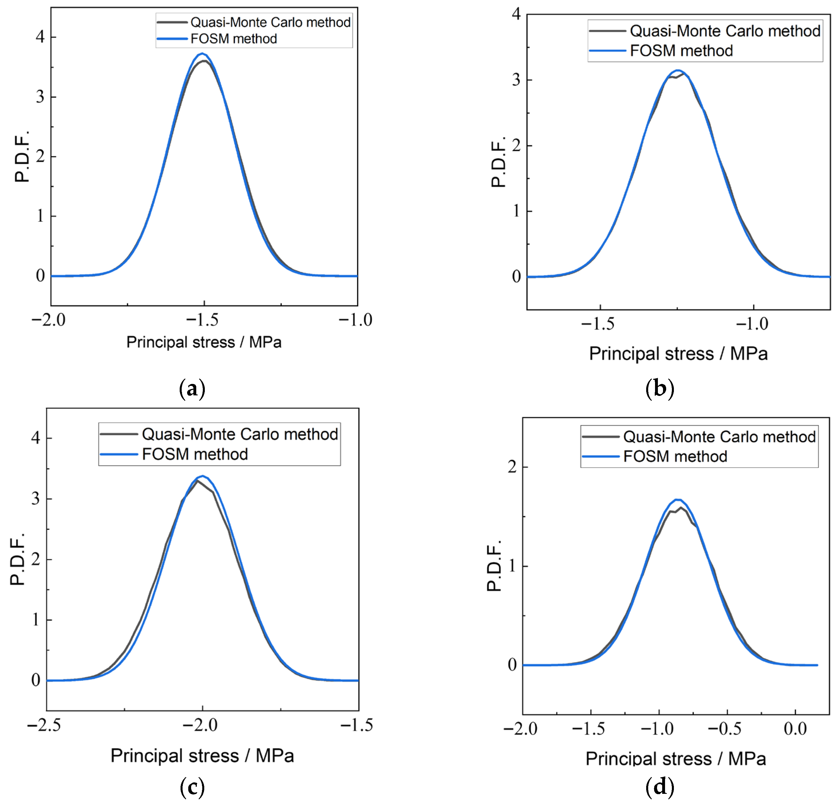
Figure 19 presents the probability density plots of the second principal stress obtained using the probability density evolution method. These plots also include the probability density based on a normal distribution derived from the mean and standard deviation of the sensitivity coefficients using the FOSM method. The probability density plots from both methods show a good fit, indicating that the first-order second-moment (FOSM) method is sufficiently accurate.

8. Impact of Creep and Shrinkage Uncertainty on Web Principal Stresses

The standard deviation of the principal stress at any given point can be determined using the approximate method illustrated in Section 7.2, and the maximum principal stress with a 95% confidence level can then be calculated based on a normal distribution assumption.

The stress analysis results in web path of the segment in Figure 12 are shown in Figure 20. On this segment, the cable is anchored near the web top, and the stress path, including the anchorage boss, is shown in Figure 12. The stresses in Figure 20 were calculated using the CEB-FIB creep and shrinkage model. When comparing the 95% confidence level stresses with the mean stresses in Figure 20, the difference between the two is larger 20 years after bridge completion than at the time of the bridge completion. This indicates that the effect of uncertainty in the creep and shrinkage coefficients on stress is magnified over time. From Figure 20d, the maximum increase in principal stress is 0.43 MPa when considering the 95th percentile compared to the mean stress.

Figure 21 compares the mean principal stresses at 20 years after bridge completion obtained from the CEB-FIB90 and B4 creep and shrinkage models on the stress path, while Figure 22 compares the 95% confidence level stresses. The mean principal stress for the CEB model has a maximum value of 0.098 MPa, while the B4 model’s maximum principal tensile stress is 0.254 MPa, with a difference of 0.156 MPa between the two mean values.

When considering a 95% confidence level, the maximum principal stress for the CEB model is 0.372 MPa, and the B4 model’s maximum principal tensile stress is 0.676 MPa. The difference between these two values is 0.304 MPa. When uncertainty (95% confidence level) is considered, the maximum principal stress increases by 0.274 MPa for the CEB model and 0.422 MPa for the B4 model compared to the mean.

The combined impact of model selection and parameter uncertainty can be seen by comparing the 95% quantile stress from the B4 model (0.676 MPa) with the mean stress from the CEB model (0.098 MPa). This results in a total difference of 0.578 MPa. This represents approximately 23% of the material’s design tensile strength (2.48 MPa), a significant portion given the low tensile capacity of concrete. Therefore, it is crucial to consider a more conservative creep and shrinkage model and account for its uncertainty in the long-term crack resistance analysis of the structure.

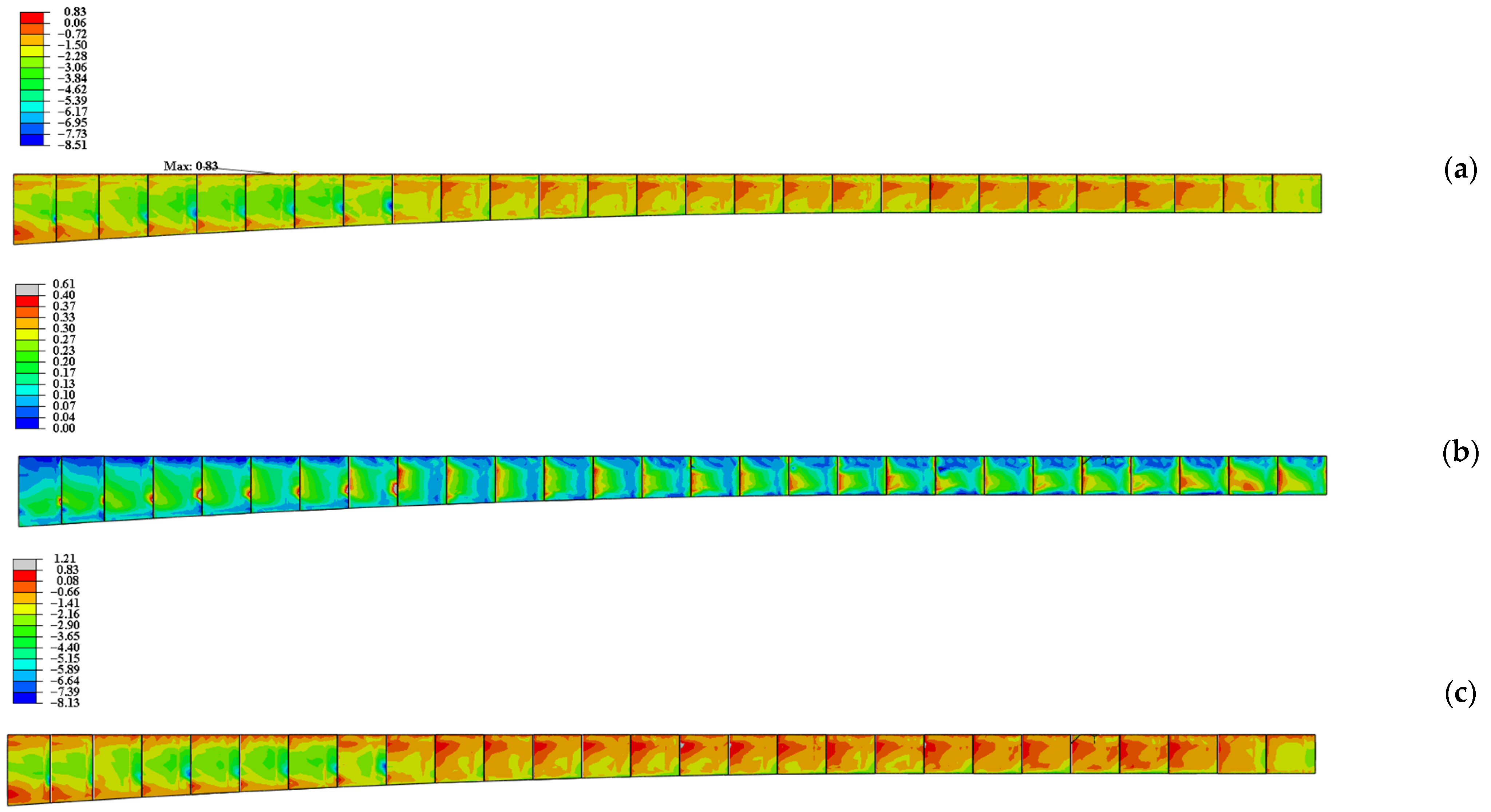
To identify potential cracking risks during long-term operation, Figure 23 shows the mean principal stress, standard deviation of the principal stress, and the 95% confidence level principal stress derived from the B4 shrinkage model after 20 years. As shown in Figure 23a, the maximum principal tensile stress is greater in the top of the web the root of the cantilever segment. The maximum principal tensile stress at the 50th percentile is 0.835 MPa.

Figure 23b shows that the standard deviation of the principal stress from creep and shrinkage is approximately periodic along the span, with each segment representing one cycle. The standard deviation is highest at the root of a segment and lowest near the end of the cantilever. This distribution pattern is similar to the vertical normal stress, which suggests that the uncertainty in creep and shrinkage might be dominated by the uncertainty in the vertical normal stress.

A comparison of Figure 21d and Figure 23c reveals that the distribution of the principal tensile stress at a 95% confidence level is similar to that at a 50% confidence level. However, when considering a 95% confidence level, the maximum principal tensile stress increases from 0.83 MPa to 1.21 MPa, an increase of 0.38 MPa. This shows that considering the uncertainty of creep and shrinkage parameters has a significant impact on the web’s crack resistance evaluation.

The combined impact of model selection and parameter uncertainty leads to a difference of 0.578 MPa between the 95% quantile principal tensile stress from the B4 model (0.676 MPa) and the mean stress from the CEB model (0.098 MPa), equivalent to about 23% of the concrete’s design tensile strength. Such a stress increment is sufficient to change a section from a safe to a cracked state under service conditions.

9. Conclusions

Based on the probabilistic analysis of the long-term effects of creep and shrinkage on an extradosed bridge using beam and solid element models, the following conclusions are drawn:

(1)

Beam element models are insufficient for accurately assessing stress in disturbed regions (D-regions) of complex box girders, such as areas near tendon anchorages. Compared to high-fidelity solid element models, beam models underestimate stress concentrations, leading to a non-conservative evaluation of crack resistance.

(2)

Solid element models predict greater long-term deflections and exhibit higher sensitivity to time-dependent parameters. For the analyzed case of an extradosed bridge with a main span of 230 m, the solid model predicted a long-term deflection mean value 14% greater than the beam model. More significantly, the sensitivity of the deflection to creep and shrinkage parameters was 34–44% higher in the solid model, indicating that beam models severely underestimate the variability and uncertainty of long-term deformations.

(3)

The proposed probabilistic framework, combining the First-Order Second-Moment (FOSM) method with solid element analysis, is both accurate and computationally efficient. The FOSM method produced results with standard deviations within 7.5% of the computationally expensive quasi-Monte Carlo sampling method, making it a feasible approach for complex models.

(4)

The influence of creep and shrinkage uncertainty on the direction of principal stresses is minimal. Our analysis showed that variations in time-dependent parameters changed the principal stress direction by a negligible amount (cosine values > 0.99). This finding validates the use of a simplified scalar FOSM approach for principal stress analysis, which yields standard deviations with less than 3% error compared to a more rigorous matrix-based sampling method.

(5)

The choice of creep and shrinkage model and its inherent parameter uncertainties have a significant impact on the long-term crack resistance assessment. Considering these uncertainties increased the 95% quantile principal tensile stress by 8–21% compared to the mean value. The combined effect of model selection and parameter uncertainty can account for a stress difference of up to 0.58 MPa, which is approximately 23% of the concrete’s design tensile strength, highlighting the critical need to account for these factors in design.

(6)

This study demonstrates that the integration of the FOSM method with high-fidelity solid element models can drastically reduce the computational burden of uncertainty analysis while maintaining high accuracy. The proposed approach effectively enables whole-bridge probabilistic analysis with solid models—previously considered computationally prohibitive—thereby representing a substantial advancement in probabilistic structural assessment for long-span prestressed concrete bridges.

This study is limited to the material uncertainty of creep and shrinkage. Future work will extend the framework to include structural modeling uncertainty, alternative construction schemes, environmental variations, hydration heat effect [40], and grouting quality [41], which may also influence long-term bridge performance.

References

1. Neville, A.M.; Dilger, W.H.; Brooks, J.J. Creep of Plain and Structural Concrete; Construction Press: London, UK, 1983. [Google Scholar]
2. Bažant, Z.P.; Baweja, S. Creep and shrinkage prediction model for analysis and design of concrete structures: Model B3. Mater. Struct. 2000, 33, 669–682. [Google Scholar]
3. Al-Manaseer, A.; Lam, J.P. Statistical evaluation of shrinkage and creep models. ACI Mater. J. 2005, 102, 170–176. [Google Scholar] [CrossRef] [PubMed]
4. Fanourakis, G.C. A study of the creep and shrinkage provisions of international codes of practice. J. S. Afr. Inst. Civ. Eng. 2011, 53, 2–13. [Google Scholar]
5. Fanourakis, G.C.; Ballim, Y. A comparative study of international concrete creep and shrinkage prediction models. Mag. Concr. Res. 2013, 65, 57–67. [Google Scholar]
6. Li, J.; Chen, J.B. Stochastic Dynamics of Structures; John Wiley & Sons: Hoboken, NJ, USA, 2009. [Google Scholar]
7. Hasofer, A.M.; Lind, N.C. An exact and invariant first-order reliability format. J. Eng. Mech. Div. 1974, 100, 111–121. [Google Scholar] [CrossRef]
8. Shah, A.; Haq, E.; Khan, S. Analysis and Design of Disturbed Regions in Concrete Structures. Procedia Eng. 2011, 14, 3317–3324. [Google Scholar] [CrossRef]
9. Schlaich, J.; Schäfer, K.; Jennewein, M. Toward a consistent design of structural concrete. PCI J. 1987, 32, 74–150. [Google Scholar] [CrossRef]
10. Oh, B.H.; Lee, K.C.; Lee, Y.J. Finite element analysis of disturbed regions in prestressed concrete structures. Eng. Struct. 2010, 32, 3848–3859. [Google Scholar]
11. Geng, Y.; Wang, Y.; Deng, M. Finite element analysis of disturbed regions in deep beams and box-girders based on the principle of minimum potential energy. Eng. Struct. 2012, 36, 1–11. [Google Scholar]
12. Liu, J.; Wang, J.; Zhang, Z.; Chen, Y. Comparative study on long-term performance of prestressed concrete box girder bridges using beam and solid finite element models. J. Bridge Eng. 2017, 22, 04017045. [Google Scholar]
13. Yang, Y.; Deng, Z.; Chen, G. Comparative study on long-term behavior of prestressed concrete continuous box girder bridges using different finite element models. Adv. Concr. Constr. 2019, 8, 1–18. [Google Scholar]
14. Jiang, C.; Wu, C.; Chen, J.; Zhuang, X. Time-dependent reliability analysis of corroding prestressed concrete bridges using polynomial chaos expansion. J. Mater. Civ. Eng. 2018, 30, 04018253. [Google Scholar]
15. Do, P.Q.; Kim, J.; Lee, D. Application of Kriging surrogate model for time-dependent reliability analysis of pre-stressed concrete bridges. KSCE J. Civ. Eng. 2019, 23, 1899–1909. [Google Scholar]
16. Nowak, A.S.; Collins, K.R. Reliability of Structures, 2nd ed.; CRC Press: Boca Raton, FL, USA, 2012. [Google Scholar]
17. Ghosn, M.; Moses, F.; Frangopol, D.M. Reliability-based performance evaluation of bridges. In Bridge Engineering Handbook, 2nd ed.; CRC Press: Boca Raton, FL, USA, 2010. [Google Scholar]
18. Lu, Z.; Zhang, Z.; Zheng, J. Time-dependent reliability analysis of long-span bridges considering uncertainties of creep and shrinkage models. Struct. Saf. 2019, 77, 77–87. [Google Scholar]
19. Yang, I.H. Probabilistic analysis of creep and shrinkage effects in PSC box girder bridges. KSCE J. Civ. Eng. 2003, 7, 275–284. [Google Scholar] [CrossRef]
20. Sun, Z.; Chen, Q.; Li, C. Probabilistic analysis of long-term deflection of prestressed concrete bridges considering creep and shrinkage model uncertainty. J. Civ. Eng. Manag. 2020, 26, 570–580. [Google Scholar]
21. Chen, T.; Deng, H.; Xu, X.; Deng, Z. Long-term performance analysis of concrete box girder bridge based on random parameters and creep models. Adv. Struct. Eng. 2017, 20, 143–154. [Google Scholar]
22. Huang, J.X.; Liu, P.; Yu, Z.W. Bayesian inference with finite element analysis for concrete structural creep and shrinkage prediction. Eng. Struct. 2025, 330, 119885. [Google Scholar] [CrossRef]
23. Guo, T.; Zhu, R.Z.; Lu, S. Long-term behavior of the self-centering post-tensioned concrete frame with web friction devices: Experimental and numerical models. J. Build. Eng. 2025, 111, 113478. [Google Scholar] [CrossRef]
24. Stewart, M.G.; Mullard, J.A. Spatial variability of concrete properties and its effect on the reliability of reinforced concrete corrosion-affected structures. Cem. Concr. Compos. 2007, 29, 395–404. [Google Scholar]
25. Fang, F.K.; Wang, Y. Number-Theoretic Methods in Statistics; Science Press: Washington, DC, USA, 1996. (In Chinese) [Google Scholar]
26. Li, J.; Chen, J.B. The Number Theoretical Method in Response Analysis of Nonlinear Stochastic Structures. Comput. Mech. 2007, 39, 693–708. [Google Scholar] [CrossRef]
27. Chen, J.B.; Ghanem, R.; Li, J. Partition of the probability-assigned space in probability density evolution analysis of nonlinear stochastic structures. Probabilistic Eng. Mech. 2009, 24, 27–42. [Google Scholar] [CrossRef]
28. Dassault Systèmes. Abaqus/CAE User’s Guide (Version 2016); Dassault Systèmes SIMULIA Corp.: Johnston, RI, USA, 2016. [Google Scholar]
29. Comité Euro-International du Béton. CEB-FIP Model Code 1990: Design Code; Thomas Telford Publishing: London, UK, 1993. [Google Scholar]
30. Ministry of Transport of China. Code for Design of Highway Reinforced Concrete and Prestressed Concrete Bridges and Culverts; JTG 3362-2018; China Communications Press: Beijing, China, 2018. (In Chinese) [Google Scholar]
31. Bažant, Z.P.; Wendner, R. RILEM draft recommendation: TC-242-MDC multi-decade creep and shrinkage of concrete: Material model and structural analysis Model B4 for creep, drying shrinkage and autogenous shrinkage of normal and high-strength concretes with multi-decade applicability. Mater. Struct. 2015, 48, 753–770. [Google Scholar]
32. Zhu, B. The Finite Element Method: Fundamentals and Applications in Civil, Hydraulic, Mechanical and Aeronautical Engineering; John Wiley & Sons: Hoboken, NJ, USA, 2018. [Google Scholar]
33. Wu, Y.; Chen, Y.; Zeng, J.; Jiang, Y.; Liu, Z. Long-Term Performance Analysis of Steel–Concrete Composite Beams Based on Finite Element Model Updating. Buildings 2025, 15, 1374. [Google Scholar] [CrossRef]
34. Santos, I.C.; Brito, J.L.V.; Caetano, E.S. Uncertainty quantification: Data assimilation, propagation and validation of the numerical model of the Arade river cable-stayed bridge. Struct. Infrastruct. Eng. 2022, 18, 1410–1427. [Google Scholar] [CrossRef]
35. Yang, Y.; Peng, J.; Liu, X.; Cai, S.C.S.; Zhang, J. Probability analysis of web cracking of corroded prestressed concrete box-girder bridges considering aleatory and epistemic uncertainties. Eng. Struct. 2021, 228, 111486. [Google Scholar] [CrossRef]
36. Poeta, A.; Micozzi, F.; Gioiella, L.; Dall’Asta, A. A case study for the reliability evaluation of an existing prestressed bridge according to current Standard. CE Pap. 2023, 6, 36–42. [Google Scholar] [CrossRef]
37. Yang, I.H. Uncertainty and sensitivity analysis of time-dependent effects in concrete structures. Eng. Struct. 2007, 29, 1366–1374. [Google Scholar] [CrossRef]
38. Bažant, Z.P.; Wendner, R. Optimization method, choice of form and uncertainty quantification of Model B4 using laboratory and multi-decade bridge databases. Mater. Struct. 2015, 48, 771–796. [Google Scholar] [CrossRef]
39. Li, S.; Yang, Y.; Pu, Q.; Yang, D.; Sun, B.; Li, X. Three-dimensional nonlinear creep and shrinkage effects of a long-span prestressed concrete box girder bridge. Struct. Concr. 2019, 20, 638–649. [Google Scholar] [CrossRef]
40. Wang, T.; Cai, J.; Feng, Q.; Jia, W.; He, Y. Experimental Study and Numerical Analysis of Hydration Heat Effect on Precast Prestressed Concrete Box Girder. Buildings 2025, 15, 859. [Google Scholar] [CrossRef]
41. Galano, S.; Losanno, D.; Parisi, F. Numerical Simulation of Post-Tensioned Concrete Girders with Defective Grouting Including Local Stress–Strain Tendons Response. Struct. Concr. 2025, 25, 4515–4536. [Google Scholar] [CrossRef]
Figure 1. Front view of the case bridge (dimension in m).
Buildings 15 03973 g001
Figure 2. Cross-section of the main girder (dimension in cm).
Buildings 15 03973 g002
Figure 3. Cross-section of the pylon (dimension in cm).
Buildings 15 03973 g003
Figure 4. Geometric model of a bridge using the beam element.
Buildings 15 03973 g004
Figure 5. Parametric modeling of girder segment with varying Cross-Sections using Tekla and Grasshopper.
Buildings 15 03973 g005
Figure 6. Solid bridge model of the case bridge during cantilever construction.
Buildings 15 03973 g006
Figure 7. Stress Paths in Inclined Web for comparing different meshing.
Buildings 15 03973 g007
Figure 8. Compare of normal stress produced by different meshing.
Buildings 15 03973 g008
Figure 9. Evolution of (a) creep coefficient (a,b) shrinkage strain over time.
Buildings 15 03973 g009
Figure 10. Comparison of mean long-term mid-span deflection: beam vs. solid analysis.
Buildings 15 03973 g010
Figure 11. Half of the cantilever structure after tensioning cable S16. S1–S16: Cable numbers. 0#–23# Beam segment numbers. The cross-section of the beam segment marked in green is shown in Figure 12.
Buildings 15 03973 g011
Figure 12. Stress observation path on the inner web.
Buildings 15 03973 g012
Figure 13. Inner web stress comparison: solid element vs. beam analysis (a) longitudinal normal stress, (b) shear stress, (c) vertical normal stress, (d) principal stress.
Buildings 15 03973 g013
Figure 14. Girder deflection during construction: mean, maximum, and minimum sample values (the beam element model).
Buildings 15 03973 g014
Figure 15. Effect of the variation in bridge parameters on the maximum deflection during construction.
Buildings 15 03973 g015
Figure 16. Comparison of probability densities for bridge deflection during construction: two probabilistic analysis methods (beam element model).
Buildings 15 03973 g016
Figure 17. Evolution of the mean values of the long-term deformation obtained from the three shrinkage-creep models.
Buildings 15 03973 g017
Figure 18. 95% Confidence Interval for Long-term Deflection of Based on Solid Element Analysis (3 Creep-Shrinkage Models), (a) CEB Model, (b) B3 Model, (c) B4 Model.
Buildings 15 03973 g018
Figure 19. Comparison of Principal Stress Probability Densities from Two Analysis Methods: (a) Point A, (b) Point B, (c) Point C, (d) Point D.
Buildings 15 03973 g019
Figure 20. Mean and 95% quantile stress on the web at bridge completion and after 20 years of bridge completion obtained from the CEB and B4 model: (a) longitudinal normal stress, (b) shear stress, (c) vertical normal stress, (d) principal stress.
Buildings 15 03973 g020
Figure 21. Mean stress on the web under two creep-shrinkage models after 20 years of bridge completion: (a) longitudinal normal stress, (b) shear stress, (c) vertical normal stress, (d) principal stress.
Buildings 15 03973 g021
Figure 22. 95% quantile stress on the web under two creep-shrinkage models after 20 years of bridge completion: (a) longitudinal normal stress, (b) shear stress, (c) vertical normal stress, (d) principal stress.
Buildings 15 03973 g022
Figure 23. Contour of the principal stress in the web considering uncertain creep and shrinkage from the B4 model (After 20 Years of bridge completion): (a) mean value (b) standard derivation (c) 95% quantile value.
Buildings 15 03973 g023