1. Introduction
Structural damage detection is an important research direction in structural health monitoring (SHM), with the core goal of preventing sudden structural damage, thereby avoiding casualties and significant economic losses. The structural safety assessment in current engineering practice relies heavily on expert judgment and on-site visual inspection. However, manual inspection is not only time-consuming and labor-intensive but also greatly influenced by subjective factors, and the safety assessment results given by different inspectors may vary [
1,
2]. In recent years, structural damage identification methods based on vibration characteristics have received widespread attention due to their flexible measurement, economic efficiency, and non-destructive detection methods [
3,
4,
5]. This type of method collects the vibration response signals of the structure under external excitation, extracts its modal parameters, and analyzes the changes in modal parameters (such as natural frequency, mode shape, or damping) to determine potential damage to the structure [
6,
7]. Previous studies have shown that frequency-based damage identification methods have been successfully applied for damage detection in composite material structures [
8,
9]. Research based on modal features has found that local damage can lead to irregularities in the vibration mode [
10], and this irregularity is more significant when the degree of damage is greater [
11,
12]. However, in actual modal testing, it is often difficult to identify minor damage due to changes in natural frequency and mode shape [
13]. As the second derivative of the vibration mode, the modal strain energy (MSE) is more sensitive to changes in structural response and is therefore often used as a damage indicator to accurately locate and estimate the extent of damage [
6,
14,
15,
16,
17]. It has been suggested that the element modal strain-based method can be more advantageous than the traditional modal curvature-based method, particularly in scenarios with sparse measurement data [
18]. However, it is difficult to obtain high-order modal data in engineering practice, and the measured signals are often accompanied by noise interference [
19]. To mitigate the impact of noise on damage identification results, it is necessary to introduce effective information processing tools. Artificial neural network (ANN), as an intelligent algorithm with feature extraction capability, can extract key features of structural damage from complex data as well as filter out irrelevant or interfering information, thereby improving the accuracy and noise resistance of damage detection [
20].
The application of ML in SDD has evolved significantly. Beyond the early and widely used BP neural networks [
21,
22], other sophisticated ML algorithms have been successfully employed. For instance, Support Vector Machines (SVMs) have been utilized for their effectiveness in high-dimensional classification problems [
23], while ensemble methods like Random Forests have shown robustness in feature importance analysis and damage prediction [
24]. However, these traditional ML methods often require careful manual feature engineering, which can be labor-intensive and subjective [
25,
26]. The recent advent of deep learning, a subset of ML, has revolutionized feature extraction by enabling the automatic learning of hierarchical features directly from raw or minimally pre-processed data [
27]. Among deep learning architectures, CNNs have demonstrated exceptional performance in processing data with grid-like topology, such as images and time-series signals converted into 2D matrices [
28,
29,
30,
31,
32]. In the context of SHM, CNNs have been effectively applied to a range of problems, from image-based crack and defect detection in bridges [
33,
34] to automated feature extraction from vibration signals [
35,
36,
37,
38,
39]. These studies underscore the potential of CNNs to handle complex, noise-contaminated data and outperform traditional methods. Nevertheless, many existing studies applying CNNs to vibration-based SDD have focused on relatively simple structural components like beams [
40] or have primarily utilized 1D CNNs for signal processing. The application of 2D CNNs to leverage the spatial distribution of element-based modal parameters for damage identification in more complex structures, such as trusses, remains less explored.
The introduction of ANN provides a new approach for damage detection in SHM. Early research often used backpropagation (BP) neural network models and has achieved certain results [
21,
22]. However, due to the limitations of the BP network itself, it still has problems such as slow convergence speed, long training time, and easy overfitting in practical applications [
25,
26]. When the structural scale is large, the sample data generated by it often have extremely high dimensions, further increasing the computational burden of model training [
40]. To overcome the shortcomings of traditional ANNs, researchers have proposed CNNs [
27]. This network achieves automatic feature extraction through multi-layer convolution and pooling structures [
28], demonstrating stronger feature capture and expression capabilities in image feature learning [
29]. Compared to BP neural networks, it has higher training efficiency and generalization performance. At present, CNNs have been widely used in font recognition, license plate detection, face recognition, and other fields [
30,
31,
32]. CNNs have also been applied to SHM, such as in crack detection [
33,
34], damage feature extraction from low-order vibration signals [
35,
36,
37,
38], and vibration-based damage detection by 1D CNNs [
39]. It is expected that CNNs can effectively overcome the influence of noise. But there are also some challenges at present, such as the simplicity of the structural model [
39,
40] (simply supported beam with rectangular section or T-shape beam) and training sample. Furthermore, for complex structures like long-span steel truss bridges, specific methodologies have been developed. For instance, model-based approaches utilizing stiffness separation for partial-model updating, as well as systematic sensitivity analyses for optimal sensor placement to enhance damage identification efficacy, have been proposed. These studies highlight the importance of tailored strategies for large-scale structures. The application of deep learning in SHM continues to evolve with diverse architectures. For instance, beyond standard CNNs, hybrid wavelet scattering networks have demonstrated effective performance in failure identification of reinforced concrete members [
41], while data-driven classifiers based on CNNs have been successfully applied for seismic failure mode detection in steel structures [
42]. These studies highlight the adaptability of deep learning to various structural types and failure modes. Building on this foundation, the present study contributes to this field by exploring a data-driven CNN approach applied to a representative steel truss model, with the aim of developing a robust method that could be scaled for application to more complex bridge structures.
In this paper, a CNN is proposed to detect damage using modal strain energy (MSE) and modal strain (MS). The difference in modal parameters before and after damage is obtained as new indices (MSED and MSD) for comparing detection results. Then the influence of different intensity noise on damage detection results is compared. Finally, the anti-noise ability of the CNN is compared with that of BP neural networks.
Based on the above background, this study aims to address the following research questions:
- (1)
Can a 2D CNN effectively utilize element-based modal parameters (MSE and MS) for accurate damage localization and quantification in a complex steel truss structure?
- (2)
How do damage indices based on the difference of modal parameters (MSED and MSD) compare with those based on raw modal parameters in terms of detection accuracy and noise robustness?
- (3)
Does the proposed CNN-based approach outperform traditional BP neural networks in terms of anti-noise capability and computational efficiency?
The hypotheses underlying this work are as follows: The use of modal parameter differences will enhance damage sensitivity and noise resistance; CNNs will demonstrate superior performance over BP networks in noisy environments and with limited training data.
2. Methods
2.1. Theoretical Background of Modal Strain Energy and Modal Strain as Damage Indices
The selection of Modal Strain Energy (MSE) and Modal Strain (MS) as damage indices is grounded in their direct physical relationship to structural stiffness and local deformation, which are altered by damage.
MSE: The MSE of an element is a measure of the energy stored in the element due to deformation under a specific vibration mode. As defined in Equation (1), it is a quadratic function of the modal displacements. Since damage in a structural element typically causes a local reduction in stiffness (e.g., simulated here by a reduced Young’s modulus), the distribution of strain energy within the structure changes. The damaged element will exhibit a decreased ability to carry strain energy, while adjacent elements may experience an increase to maintain equilibrium. This redistribution of MSE provides a sensitive indicator for locating damage. The MSE-based index is particularly powerful because it is a global quantity derived from local stiffness and mode shape information, making it more sensitive to localized damage than global parameters like natural frequencies.
MS: Modal Strain directly represents the deformation field corresponding to a specific mode shape. Damage-induced stiffness loss alters the local curvature of the mode shape, which is directly proportional to the strain. Therefore, changes in MS at the location of damage are often more pronounced than changes in the modal displacements themselves. While MSE integrates the effect of stiffness and deformation, MS offers a more direct and potentially sharper view of the local deformation anomaly caused by damage.
In this study, we utilize both indices to leverage their complementary strengths. The difference of these parameters before and after damage (MSED and MSD) is calculated to amplify the changes caused by damage and minimize the influence of the baseline structural properties, thereby enhancing the sensitivity of the input data presented to the neural network.
2.2. Overview of Methodology
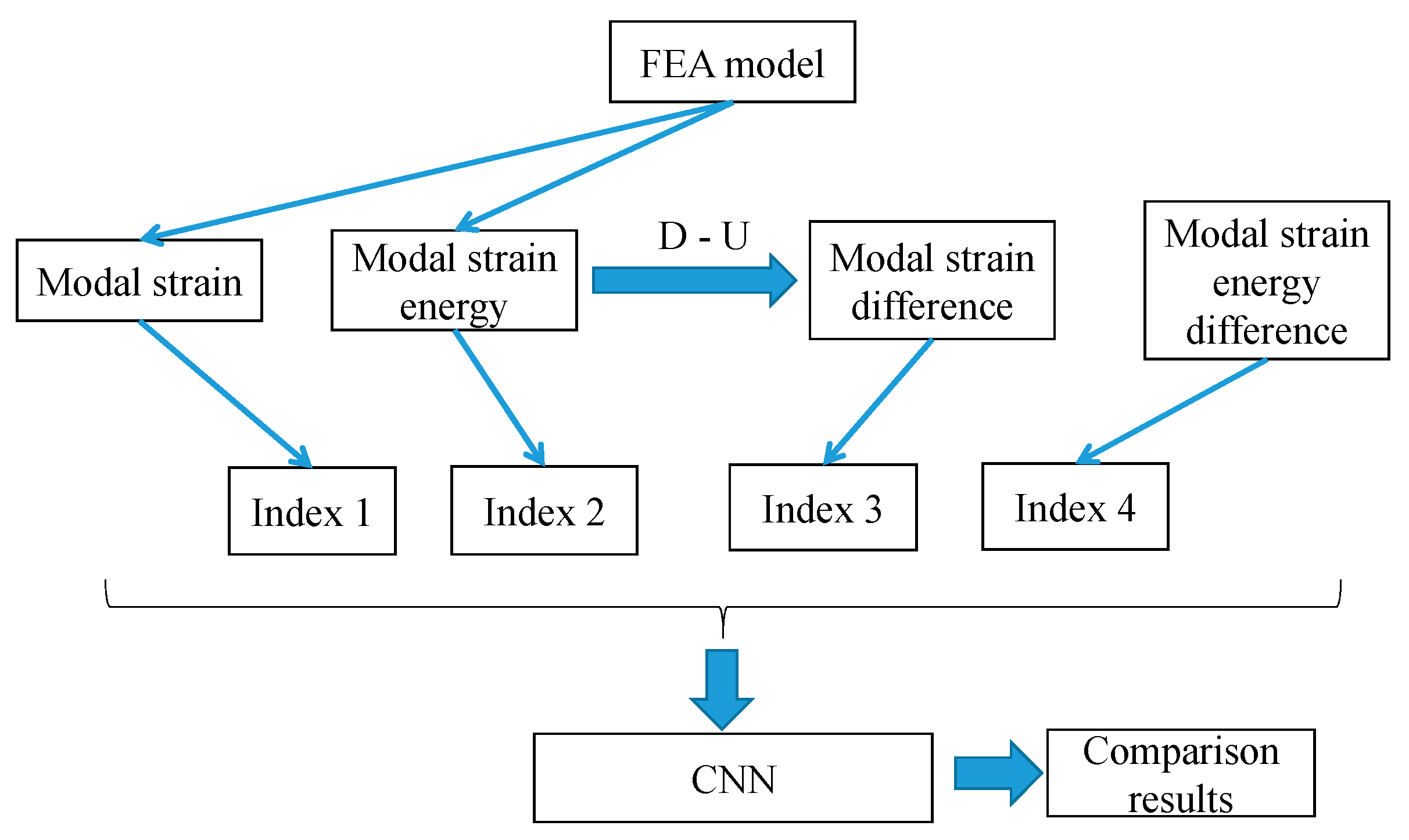
This article uses modal parameters obtained under different damage conditions (including MSE, MS, MSED, and MSD) to train a CNN and use it to predict unknown damage situations. For the convenience of model processing, the collected modal data are organized into a two-dimensional matrix form as input for the CNN. Through the feature extraction capability of the network, the CNN can identify abnormal changes from modal parameters, thereby achieving prediction of the location and level of structural damage. The overall process of damage detection based on the CNN is shown in
Figure 1.
To analyze the impact of noise on the results of structural damage detection, this paper added Gaussian white noise of different intensities to the calculated modal parameters (MSE, MS, MSED, MSD) under various damage conditions. The generation and addition process of noisy data were completed in the MATLAB R2019a (MathWorks, Natick, MA, USA) environment [
43] built-in function called awgn (Add White Gaussian Noise) to ensure a standardized approach. The noise level was defined by the signal-to-noise ratio (SNR), specified in decibels (dB). The SNR values used were 40 dB, 30 dB, 26 dB, 20 dB, and 14 dB, which correspond to noise with standard deviations approximately equal to 1%, 3%, 5%, 10%, and 20% of the maximum amplitude of the respective modal parameter signal, making the noise intensity dimensionless. These specific levels were chosen to simulate a range from mild to severe measurement noise.
2.3. Numerical Calculation and Sample
This paper uses a steel truss model (as shown in
Figure 2) with overall dimensions as follows: length 3.54 m, width 0.354 m, and height 0.354 m. Each member has a solid circular cross-section with a cross-sectional radius of 0.005 m. The material parameters of the model are set as follows: Young’s modulus 211 GPa, Poisson’s ratio 0.288, and density 7800 kg/m
3.
The damage to the rod was simulated by reducing its elastic modulus, and it was assumed that the degree of damage is proportional to the magnitude of the decrease in elastic modulus. For each unit, a total of 18 different damage levels were set, with the damage amplitude increasing from 5% to 90%, with a step size of 5%.
Adequate training samples are a prerequisite for implementing CNN training. This paper uses ABAQUS (SIMULIA Inc., Providence, RI, USA) for parametric analysis to obtain modal parameters of the structure under different damage conditions, which were used as input data for the CNN; the output of the CNN was the location and degree of damage. Firstly, a finite element model of the non-destructive structure (see
Figure 2) was established, treating each member as a set of elements and assigning corresponding material properties. After generating the input file through ABAQUS, damage was introduced into the member by reducing the Young’s modulus. Subsequently, the input file of the lossless structure was automatically modified using a self-written Python (Version 3.12) script and submitted to ABAQUS for analysis of different damage scenarios. After the analysis was completed, the required modal parameters were extracted and saved as CNN training sample data files.
The first-order MSE and MS of the structure were used. MSE was obtained by extracting the ABAQUS field variable (ELSE), and MS was obtained by extracting the ABAQUS field variable (E11). The formula of the
i-th MSE of
j-th element,
, was determined as follows [
14]:
where
and
are the
i-th-order modal shape and stiffness matrix of the
j-th element.
The first-order modal parameters were selected for this study for two main reasons. Firstly, from a practical measurement perspective, lower-order modes are significantly easier to excite and accurately measure in real-world structures compared to higher-order modes, which often require more complex excitation and are more susceptible to contamination by noise. Secondly, while higher-order modes may offer greater spatial resolution for damage localization, the first-order mode typically contains the majority of the structural strain energy and has been demonstrated to be sufficiently sensitive to damage for the purposes of this study, especially when using sensitive damage indices like modal strain energy. The use of a single, easily obtainable mode aligns with the goal of developing a practical and efficient damage detection method. Future work will explore the potential benefits of incorporating higher-order modes or combinations thereof.
Firstly, the detection of the damage location is studied. In order to compare the effects of training data on damage detection, a variety of training sets are set up for network training. In this paper, there are 101 rods in the structure. The modal parameters of a rod damage will be obtained as a sample, so 101 samples can be obtained for each damage level. The dataset of the CNN is shown in
Table 1, and the number of datasets is shown in
Table 2. The dataset types of the four indices mentioned in
Section 2.1 are identical.
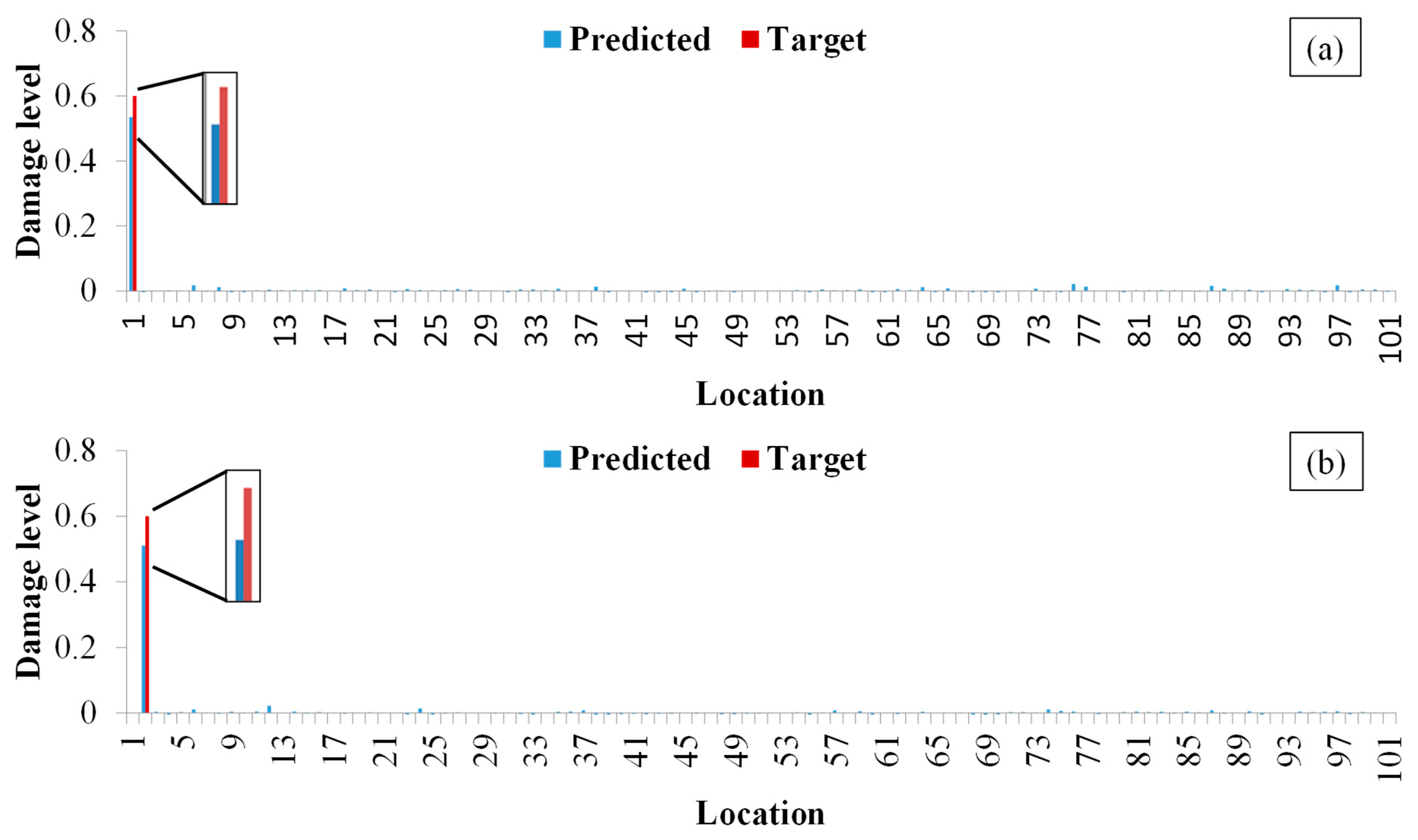
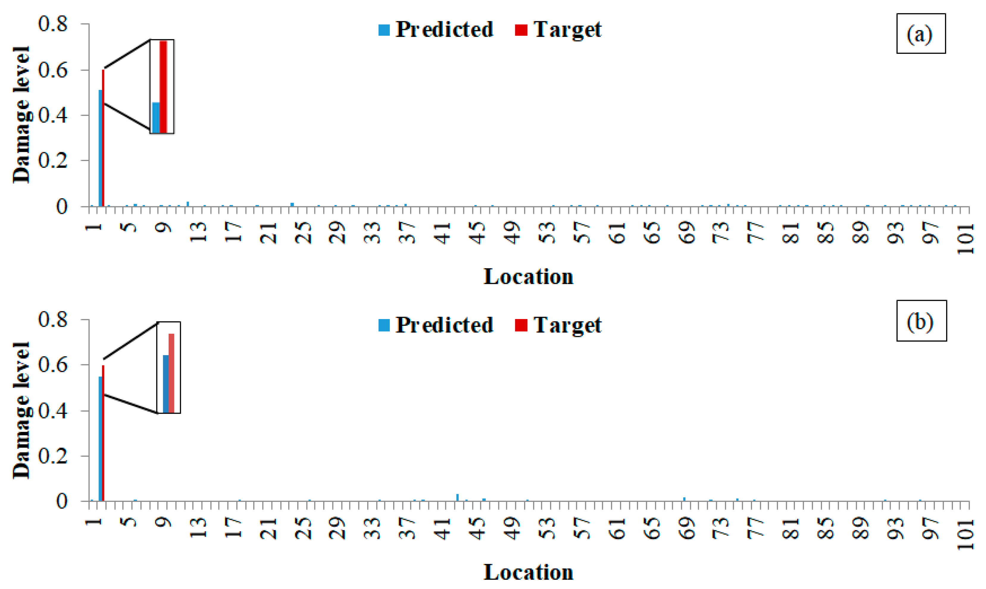
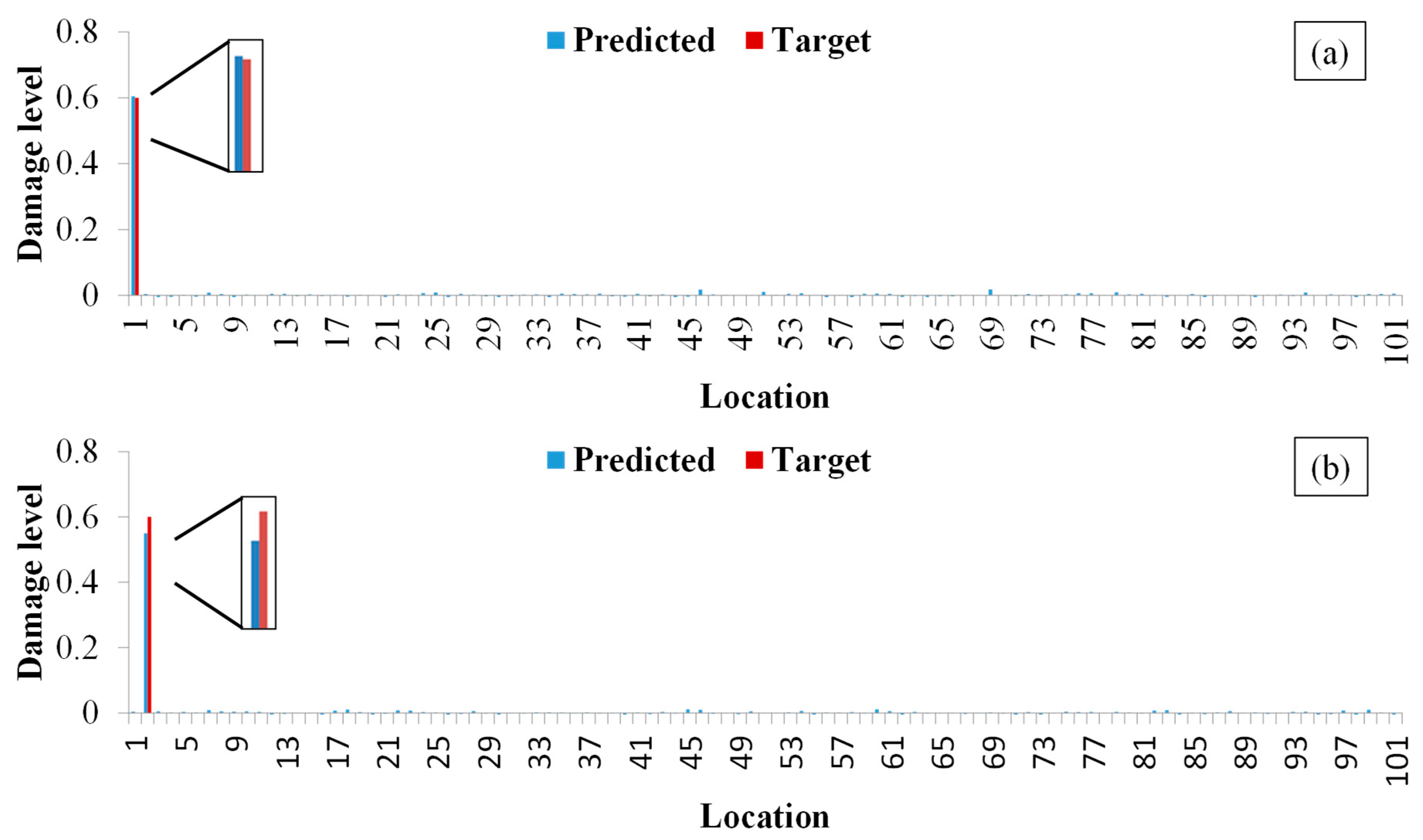
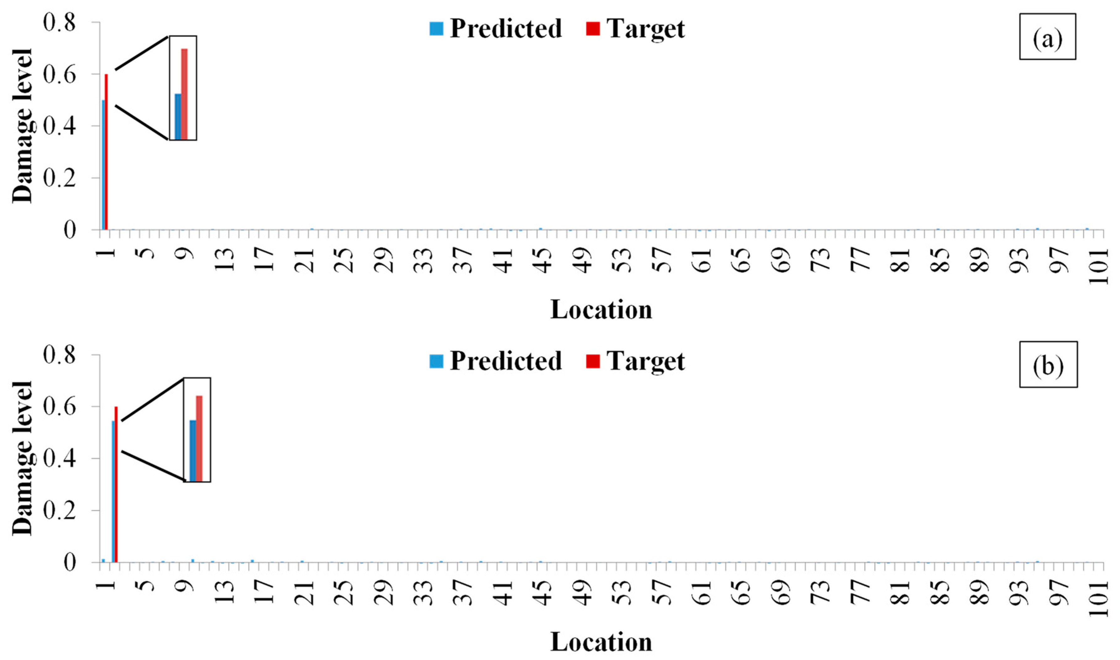
Subsequently, research was conducted on the identification of the degree of structural damage. Each unit is set with a total of 18 damage levels, with the damage amplitude increasing from 5% to 90%, with a step size of 5%. Therefore, the model includes a total of 1818 damage scenarios of 101 × 18, plus one non-destructive condition, for a total of 1819 samples. The validation set consists of data with a unit damage degree of 45% and a lossless state, totaling 102 samples; 101 samples with a unit damage of 60% were used to test the fitting performance of the CNN. A total of 1617 samples of other damage scenarios and non-destructive data were used as the training set.
2.4. Input and Output of Network
For each damage scenario, the modal strain energy of each member (a total of 101 members) was collected as input data for the CNN, and 20 zero values were added at the end, so that the input vector for each damage scenario contained 121 (101 + 20) values. Subsequently, the vector was reconstructed into an 11 × 11 matrix form and input into the CNN. This study uses a classification method to identify the location of damage, where different categories correspond to different states: the lossless state is set to 0, the first unit damage is set to 1, the second unit damage is set to 2, and so on.
The 1D vector of 101 modal values was converted into an 11 × 11 matrix by appending 20 zeros. This transformation was performed to meet the input requirements of standard 2D CNN architectures, which are optimized for grid-like data. The dimension 11 × 11 was chosen as the smallest perfect square (121) capable of holding the 101 data points. While zero-padding does not add informational content and could potentially be seen as introducing artificial boundaries, CNNs are designed to be robust to such translations through local feature detection via convolution kernels. The network learns to focus on the patterns within the meaningful data region.
In order to achieve classification and recognition of damage locations, a Softmax layer was added after the fully connected layer. The Softmax layer converts the input vector into a probability distribution using the Softmax function. Specifically, the function takes a vector
Z containing
K positive numbers as input and normalizes it into a vector
, which contains
K probability values, representing the predicted probability distribution for each category. The function is defined as shown in Equation (2).
for
j = 1…
K and
; obviously
and
. Applying this function to CNN can be used to solve multi-classification problems. For a given sample vector
x and weight vector
w, the Softmax function can calculate the prediction probability corresponding to class
j. The specific formula is as follows:
for
j = 1…
K, where
and
; moreover,
x is the output vector of the fully connected layer,
w is the connection weight between the network output and the target output, and
represents the conditional probability that the sample belongs to class
j under the condition of input
x.
For the classification task (damage location), a Softmax layer was applied after the fully connected layer to output a probability distribution across the 102 possible classes (101 damage locations + intact). The cross-entropy loss function (Equation (4)) was used to train the network [
44].
where
N represents the total number of damaged and undamaged samples,
K, represents the number of categories of damage locations,
indicates that the
i-th sample belongs to the
j-th element (damage location), and
is the output for sample
i for damage element
j. The loss represents the difference between the predicted damage and the actual damage; it was used to judge the training state (convergence or divergence) of the network.
For the regression task (damage level), the Softmax layer was replaced by a regression layer, and the mean-squared error (Equation (5)) was used as the loss function.
where
R is the number of samples,
is the target output, and
is the CNN prediction result for sample
i.
2.5. CNN
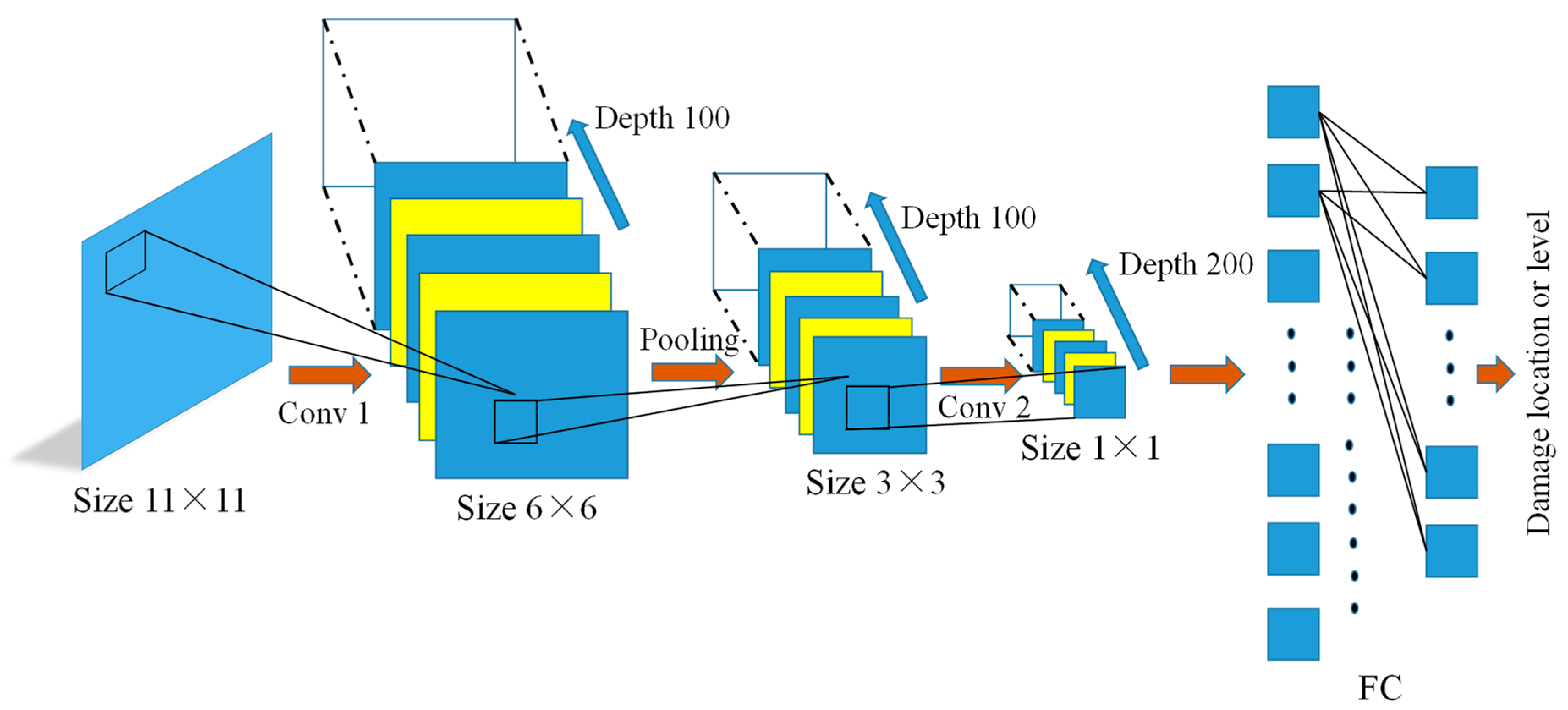
This study designed and trained a CNN using the Deep Learning Toolbox in MATLAB (MathWorks, Natick, MA, USA). The network structure includes an input layer, convolutional layer, pooling layer, activation layer, fully connected layer, and output layer (classification layer or regression layer). For classification tasks, a Softmax layer was added after the fully connected layer. The function of the activation function and the specific operation process of convolution and pooling are shown in
Figure 3.
4. Discussion
The achievement of optimal performance with datasets (f), (g), and (h) underscores the importance of training data diversity. These datasets, which include examples of both moderate and severe damage levels, provide the CNN with a broader representation of the damage feature space. This enables the model to learn a more generalized mapping function, leading to superior interpolation and extrapolation performance on unseen damage severities (10% and 60%) compared to models trained on narrower ranges of damage levels. The pronounced improvement of MSED over MSE, contrasted with the more modest gain of MSD over MS, can be attributed to the fundamental mathematical properties of the indices. MSE, being a quadratic function of the mode shape, contains strong baseline components related to element stiffness. The difference operation (MSED) effectively filters out this baseline, yielding a signal highly concentrated on damage-induced changes. In contrast, MS is a linear function already directly representing local deformation, making it inherently sensitive. Therefore, while MSD still improves robustness, the relative gain is less dramatic than the transformation achieved by converting MSE to MSED.
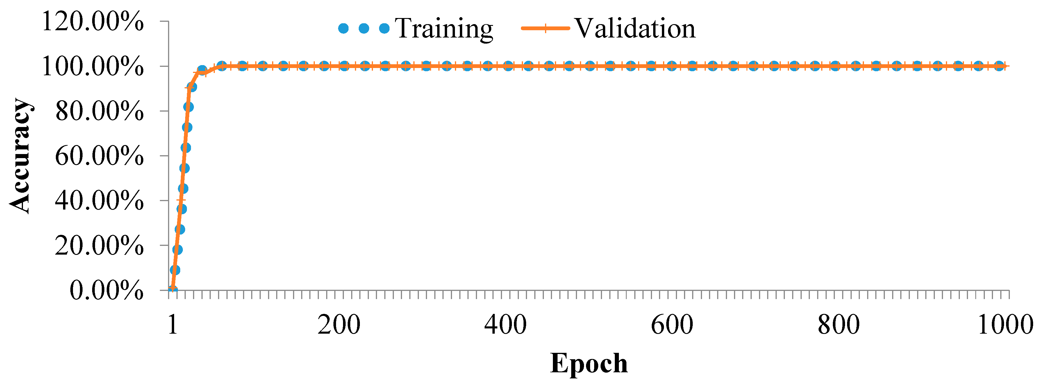
The achievement of 100% classification accuracy for damage location under specific conditions (e.g., using MSED/MSD with certain training sets) warrants discussion. While perfect accuracy is rare in practice, it can occur in controlled numerical studies where the primary source of uncertainty (measurement noise) is absent or minimal, and the damage index is highly sensitive. The fact that accuracy decreased significantly under higher noise levels (
Section 3.3) and when using fewer sensitive indices (
Section 3.1) confirms that the CNN was learning non-trivial feature-damage relationships rather than benefiting from a trivial encoding of the solution in the input data structure. The 2D input format was chosen to leverage the spatial-feature learning capability of the CNN, not to pre-code location information.
While this study demonstrates the effectiveness of a CNN-based approach on a laboratory-scale truss model, its translation to real-world long-span truss bridges would need to address challenges such as environmental variability and limited sensor coverage. In such scenarios, the integration of the proposed method with model-based techniques like stiffness separation for model updating or strategies for optimal sensor placement derived from sensitivity analysis could be a promising future direction to combine the strengths of both physics-based and data-driven paradigms.
It is noteworthy that the BP network and the CNN utilized different activation functions (tansig and Leaky ReLU, respectively). This choice was intentional, reflecting the standard and most effective practices for each architecture. The tansig function is a conventional choice for shallow BP networks, ensuring our results are consistent with the historical literature. In contrast, Leaky ReLU is essential for training deeper CNNs effectively by preventing the vanishing gradient problem. The comparison presented here, therefore, evaluates each network type in its recommended configuration, aiming to compare their inherent strengths rather than enforcing an identical but potentially suboptimal setup. This approach provides a more practical assessment of which architectural paradigm is better suited for this specific task.
The reviewer rightly raised a concern regarding the potential for overfitting, given the complexity of our CNN architecture relative to the size of some training sets (e.g., ~102 samples). Our analysis of the training and validation loss curves for these scenarios shows that while the training loss continued to decrease, the validation loss plateaued early in the training process. This confirms that the model capacity was indeed greater than necessary for the small datasets. However, the use of early stopping based on the validation set effectively prevented the model from overfitting to the training data, as training was halted at the point of best validation performance. Furthermore, the addition of noise during training acted as a regularizer. Therefore, while the models trained on very small datasets may not have reached their full potential, the reported performance on the independent test set is a legitimate measure of their generalization capability under these constrained conditions. For practical applications, larger datasets would undoubtedly be beneficial.
5. Limitations and Future Work
Despite the promising results, this study has several limitations that should be acknowledged. Firstly, the proposed method was validated using a numerical model under simulated free vibration conditions. While this allows for a controlled investigation, it does not account for practical challenges such as ambient vibrations, temperature effects, measurement errors beyond simulated noise, and the quality of real-world modal identification. Future work will involve experimental validation on a physical laboratory model and the analysis of field data from actual structures to assess the method’s performance under realistic conditions.
Secondly, the current study primarily focuses on single damage scenarios. The capability of the CNN to identify and quantify multiple concurrent damages requires further investigation. This is a more complex but practically important problem.
Thirdly, the truss model, though more complex than the simple beams often used in related studies, is still a simplified representation of real-world bridge structures. The performance of the method when applied to large-scale, complex structures with different types of members (e.g., beams, slabs) and boundary conditions remains an open question.
Lastly, the method relies on the availability of modal data from the undamaged (baseline) state of the structure to calculate the difference indices (MSED, MSD). In cases where such baseline data are unavailable, alternative strategies would need to be developed.
Future research will address these limitations by (1) conducting experimental verification; (2) extending the framework to multi-damage detection; (3) applying the method to more complex and large-scale finite element models and real bridge monitoring data; and (4) exploring baseline-free damage detection techniques.
