Analytic Solutions for the Stationary Seismic Response of Three-Dimensional Structures with a Tuned Mass-Inerter Damper and Bracket

Abstract

The ultimate goal of research on seismic mitigation technologies is engineering application. However, current studies primarily focus on the application of dampers in planar structures, while actual engineering structures are three-dimensional (3D) in nature. A type of damper, making up tuned mass dampers (TMDs) and inerters, has excellent vibration mitigation performance and needs brackets to connect to structures. In this work, a coupled dynamic model of an energy dissipation system (EDS) comprising a TMD, an inerter, a bracket, and a 3D building structure is presented, along with analytical solutions for stochastic seismic responses. The main work is as follows. Firstly, based on D’Alembert’s dynamics principle, the seismic dynamic equations of an EDS considering a realistic damper and a 3D structure are formulated. The general dynamic equations governing the bidirectional horizontal motion of the EDS are further derived using the dynamic finite element technique. Secondly, analytical expressions for spectral moments and variances of seismic responses are obtained. Finally, four numerical examples are presented to investigate the following: (1) verification of the proposed response solutions, showing that the calculation time of the proposed method is approximately 1/500 of that of the traditional method; (2) examination of spatial effects in 3D structures under unidirectional excitation, revealing that structural seismic responses in the direction along the earthquake ground motion is approximately 10⁴ times that in the direction perpendicular to the ground motion; (3) investigation of the spatial dynamic characteristics of a 3D structure subjected to unidirectional seismic excitation, showing that the bracket parameters significantly affect the damping effects on an EDS; and (4) application of the optimization method for the damper’s parameters that considers system dynamic reliability and different weights of the damper’s parameters as constraints, indicating that the most economical damping parameters can achieve a reduction in displacement spectral moments by 30–50%. The proposed response solutions and parameter optimization technique provide an effective approach for evaluating stochastic seismic responses and optimizing damper parameters in large-scale and complex structures.

1. Introduction

Vibration control technologies [1,2] aim to adjust the vibration characteristics of structures through energy absorption or reduce seismic energy input through energy dissipation devices, thereby mitigating damage to structures subjected to strong wind or earthquakes. Currently, vibration control technologies are regarded as the most critical measures for earthquake prevention and reducing losses in the engineering field and have received extensive attention [3,4,5]. Control devices, such as base isolation [6], tuned mass dampers (TMDs) [7], viscoelastic dampers [8], friction dampers [9], inerters [10], magnetorheological dampers [11], and negative stiffness dampers [12], have been developed. They have demonstrated excellent vibration reduction performance. However, because of the complexity of building structures and external excitations, only one type of passive damper cannot perfectly control structural dynamic responses. Therefore, the combined application of multiple types of dampers has become an option to enhance the vibration control effect [13,14,15,16], making hybrid dampers a current hotspot in engineering.

Both TMDs and inerters are inertial dampers. The inertial force of a TMD is proportional to the absolute acceleration of a mass block [17], while that of an inerter is proportional to the relative acceleration at both ends of a device [18]. A TMD is a single-point type of damper that achieves the purpose of reducing structural vibration by connecting a mass element, a spring element, and a viscous element in series with building structures [19]. The mitigation performance of a TMD is related to the mass and the ratio of the nominal circular frequency of TMDs to that of building structures [20], with relatively strict application conditions [21]. Inerters are a two-terminal type of passive control device that can generate a big inerter coefficient, which plays a decisive role in vibration mitigation through certain mechanisms [5,22], with additional brackets linking buildings. Since TMDs are a single-point damper and inerters are a two-terminal one, they easily form hybrid dampers to give full play to their advantages. Giaralis et al. [23] studied the dynamic output of a high-rise structure with a hybrid damper composed of a TMD and an inerter (TMDI), and their results showed that the TMDI exhibited better damping characteristics and robustness compared to a single TMD. Zhang et al. [24] presented a hybrid damper consisting of a series-parallel layout-II inerter in parallel with a tuned spring and in series with a tuned mass and investigated the seismic response mitigation of a wind turbine tower with this type of damper. Deng et al. [25] studied the random seismic response of a high-rise structure with a hybrid damper composed of a series-parallel inerter system and a TMD. The above achievements mainly focus on the seismic performance research of hybrid dampers composed of a TMD and inerters applied to planar structures and fail to consider the issue that brackets are required when inerters are applied. However, actual engineering is spatial in nature, so it is necessary to investigate the vibration mitigation effect of hybrid damper devices combined with TMDs and inerters in practical engineering applications. The application of such hybrid damping devices requires brackets to connect with structures. In this work, the dynamic performance of a 3D structure with a hybrid damper composed of a TMD, a series layout inerter system (SLIS) [26], and a bracket in series (TMD-SLIS-B) is carried out.

The vibration reduction performance of hybrid devices composed of TMDs and inerters is significantly influenced by their mechanical parameters. Therefore, the parameters’ optimization analysis has become an important step in determining the engineering application. In light of the fixed-point theory, Hu et al. [27] researched the seismic optimization parameters of a single-degree-of-freedom structure equipped with an inerter-isolation device by H₂ and H_∞ optimization methods. The research shows that compared with traditional vibration control devices, the inerter can acquire better vibration mitigation effects without increasing the physical mass of the structure. Pan et al. [28] investigated the random dynamic response of a single-degree-of-freedom system with an inerter and presented an optimal method for the inerter’s parameter optimization. This method aims to obtain the optimal structural dynamic output and the lowest cost of an inerter. Wang et al. [29] proposed the analytical solutions for outputs of structures equipped with a tuned parallel inerter mass system (TPIMS) subjected to random earthquakes and presented an optimization method for the TPIMS’s parameters with constraints corresponding to the structural dynamic reliability and the implementation difficulty of damper parameters. The proposed parameter optimization method can obtain the economical damper parameters that satisfy safety requirements. The above research achievements provide valuable ideas for obtaining optimal damper parameters. Therefore, this work studies an optimization method for eight parameters of a TMD-SLIS-B installed in 3D structures based on the optimization method proposed in Reference [29].

It is widely acknowledged that ground motion is random, and the power spectral density function (PSDF) is described in the frequency domain form. There are numerous random seismic excitation models based on the PSDF, such as the white noise spectrum [30], the filtered white noise spectrum [31], and the double-filtered white noise spectrum (also known as the Clough–Penzien spectrum [25]). Among them, the Clough–Penzien spectrum can more effectively suppress low-frequency components through a dual-layer filtering structure, making the simulated ground motion more consistent with the characteristics of relatively prominent high-frequency components in actual earthquakes. For structures sensitive to low-frequency vibrations, such as long-period structures and long-span bridges, it can more accurately evaluate the response of structures under seismic action. The quadratic decomposition of the PSDF (QD-PSDF) [16,25,29,32] was proposed to perform response analysis for various linear structures subjected to stationary random excitations. In this work, the QD-PSDF is used to study the seismic zero-order, first-order, and second-order response spectral moments (ZFSO-RSMs) of various responses of a 3D structure with a TMD-SLIS-B under unidirectional seismic excitation modeled by Clough–Penzien excitation.

The outline of this manuscript is as follows. In Section 1, based on D’Alembert’s principle and the mechanical principles of a TMD-SLIS-B, the coupled seismic dynamic equations of the energy dissipation system (EDS) composed of a TMD-SLIS-B and a 3D building structure are first established. The dynamic finite element technology is used to acquire the real-mode vibration parameters of a bare 3D structure to form the equivalent equation of the EDS equation. In Section 2, a standardized form of the frequency domain solutions of the dynamic outputs (i.e., the bidirectional motion in the horizontal direction of structural nodes, the inter-story displacements of column components, the TMD’s vibratory displacement, the brace’s deformation, and the SLIS’s force and their change rates) is derived. Applying the QD-PSDF, the analytical solution of the ZFSO-RSMs of seismic outputs of the EDS subjected to Clough–Penzien excitation is derived. Section 3 proposes an optimization analysis method for the TMD-SLIS-B’s parameters using system dynamic reliability as the boundary condition and taking different weights of the TMD-SLIS-B’s parameters into account. In Section 4, four mathematical cases are given to validate the correctness of the presented analytic solutions for the ZFSO-RSMs of the seismic outputs of the EDS, the spatial seismic dynamic characteristics of the 3D structure under unidirectional seismic excitation, the effects of mechanical parameters of the brace in the TMD-SLIS-B on the structural vibration response, and the demonstration of the optimization method of the TMD-SLIS-B’s mechanical parameters.

2. Establishment of Seismic Equations for 3D Structures with a TMD-SLIS-B

The actual building structure is a spatial structure. In engineering, its seismic outputs in the direction of the minor axis within a plane are often investigated. For the convenience of exposition, when studying the dynamic responses of a 3D building, the direction in the minor axis within the plane of the building structure is named as the X-direction, and the direction in the major axis is named as the Y-direction, which are perpendicular to each other. In this section, the establishment of the seismic motion equation of a 3D structure with a TMD-SLIS-B under the action of seismic excitation in the X-direction is carried out.

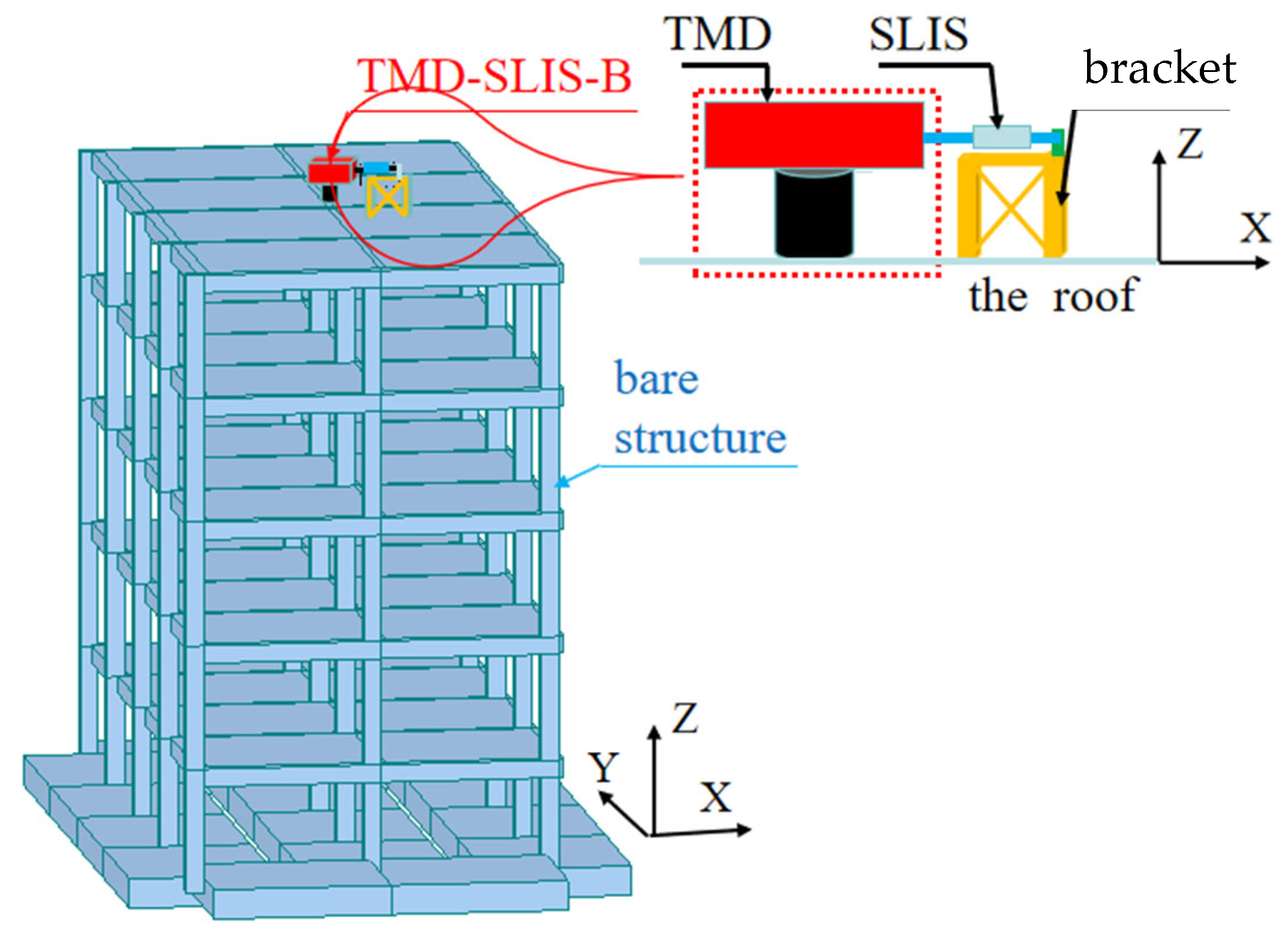
A TMD-SLIS-B is fitted to the roof of a 3D building to form an EDS, as shown in Figure 1. The EDS consists of a building structure (referred to as a bare structure) and a TMD-SLIS-B. A Cartesian spatial coordinate system is adopted for the EDS, where the X-axis and Y-axis form the horizontal coordinate system, and the Z-axis represents the height direction of the structure. The structure is subjected to seismic excitation in the X-direction, and the TMD-SLIS-B is set in the Z-X plane to suppress the seismic response in the X-direction. 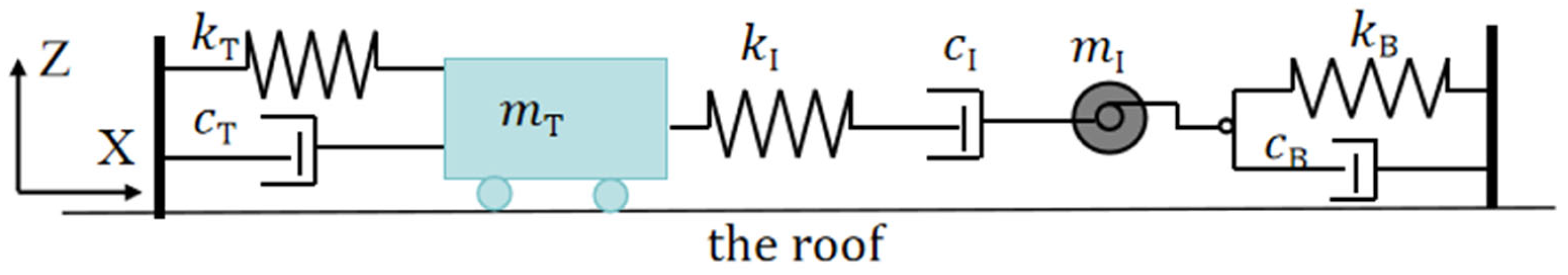Figure 2 shows the mechanical schematic diagram of the TMD-SLIS-B. Based on D’Alembert’s principle, the dynamic equations of the damping system subjected to earthquake excitation in the X-direction are formulated as

$$\mathit{M}\ddot{\mathit{x}}+\mathit{C}\dot{\mathit{x}}+\mathit{K}\mathit{x}+{\mathit{I}}_{\mathrm{D}}{m}_{\mathrm{T}}\left({\ddot{x}}_{\mathrm{T}}+{\ddot{x}}_{\mathrm{sr}}\right)=-\left(\mathit{M}\mathit{I}+{\mathit{I}}_{\mathrm{D}}{m}_{\mathrm{T}}\right){\ddot{x}}_{\mathrm{g}}$$

(1a)

$$m_{\mathrm{T}}\left({\ddot{x}}_{\mathrm{T}}+{\ddot{x}}_{\mathrm{sr}}\right)+c_{\mathrm{T}}{\dot{x}}_{\mathrm{T}}+k_{\mathrm{T}}{x}_{\mathrm{T}}+F_{\mathrm{I}}=-m_{\mathrm{T}}{\ddot{x}}_{\mathrm{g}}$$

(1b)

where M, C, and $\mathit{K}\in \mathbb{R}$^2n×2n are the mass matrix, the inherent damping matrix, and the stiffness matrix of the bare 3D building, respectively; $\ddot{\mathit{x}},\dot{\mathit{x}}$ and $\mathit{x}\in {ℝ}^{2n\times 1}$ denote the vectors of nodal displacement, nodal velocity, and acceleration of motion with respect to the ground, which are referred to in two main directions (namely, the X-direction and the Y-direction), respectively; and n denotes nodal amount of the whole 3D building. ${\ddot{x}}_{\mathrm{sr}}\in ℝ$ denotes the X-direction motion acceleration of the roof node connecting to the TMD-SLIS-B; $x_{\mathrm{T}}\in ℝ$ denotes the X-direction motion displacement of the TMD mass element, which is relative to the displacement of the connecting node in the roof, and ${\ddot{x}}_{\mathrm{T}}\in ℝ$ and ${\dot{x}}_{\mathrm{T}}\in ℝ$ are the second and first derivative of x_T with respect to time, respectively. I $\in \mathbb{R}$^2n×1 is a vector with elements 0 or 1; when the node of the structure moves along the X-direction, the responding element in I is 1; otherwise, it is 0. ${\mathit{I}}_{\mathrm{D}}$$\in \mathbb{R}$^2n×1 is a vector with elements 0 or 1; when the roof node connecting with the TMD-SLIS-B moves along the X-direction, the corresponding element in I_D is 1; otherwise, it is 0. $F_{\mathrm{I}}$ $\in \mathbb{R}$ represents the SLIS’s force; $m_{ \mathrm{T}}$,$c_{ \mathrm{T}}$, and $k_{\mathrm{T}}$$\in \mathbb{R}$ denote the mass coefficient, the viscous coefficient, and the stiffness coefficient in the TMD, respectively; and $x_{\mathrm{g}}\in ℝ$ denotes horizontal seismic acceleration in the X-direction.

In order to obtain the analytic solutions for the random seismic outputs of an EDS, establishing the relationship among the SLIS’s force, the TMD’s displacement, and the brace’s deformation is needed. Figure 3 shows the mechanical diagram of an SLIS and the brace, and the relations are described as

$$F_{ \mathrm{I}}=k_{ \mathrm{I}}{x}_{ \mathrm{I}1}=c_{ \mathrm{I}}{\dot{x}}_{ \mathrm{I}2}=m_{ \mathrm{I}}{\ddot{x}}_{ \mathrm{I}3}=k_{\mathrm{B}}{x}_{\mathrm{B}}+c_{\mathrm{B}}{\dot{x}}_{\mathrm{B}}$$

(2a)

$$x_{\mathrm{I}1}+x_{\mathrm{I}2}+x_{\mathrm{I}3}+x_{\mathrm{B}}=x_{\mathrm{T}}$$

(2b)

where $m_{ \mathrm{I}}$, $c_{\mathrm{I}}$, and $k_{\mathrm{I}}\in ℝ$ represent the designated mass coefficient of the inerter, the damping coefficient of viscous damping, and the stiffness coefficient of the spring in the SLIS, respectively; $x_{ \mathrm{I}1}$ and $x_{ \mathrm{I}2}\in ℝ$ are the deformations of the spring and the inerter, respectively; ${\dot{x}}_{ \mathrm{I}1}$ and ${\dot{x}}_{ \mathrm{I}1}\in ℝ$ are the first-order and second-order derivatives of $x_{ \mathrm{I}1}$, respectively; ${\ddot{x}}_{ \mathrm{I}2}$ denotes the second-order derivatives of $x_{ \mathrm{I}2}$; $k_{ \mathrm{b}}$ and $c_{ \mathrm{b}}\in ℝ$ are the stiffness coefficient and the damping coefficient of the bracket connecting to the roof, respectively; $x_{ \mathrm{b}}$ is the deformation of the bracket; and ${\dot{x}}_{ \mathrm{b}}$ is the first-order derivative of $x_{ \mathrm{b}}$.

According to Equations (1b) and (2a), the relation is rewritten as

$$m_{\mathrm{T}}\left({\ddot{x}}_{\mathrm{T}}+{\ddot{x}}_{\mathrm{sr}}\right)+k_{\mathrm{T}}{x}_{\mathrm{T}}+c_{\mathrm{T}}{\dot{x}}_{\mathrm{T}}+k_{\mathrm{B}}{x}_{\mathrm{B}}+c_{\mathrm{B}}{\dot{x}}_{\mathrm{B}}=-m_{\mathrm{T}}{\ddot{x}}_{\mathrm{g}}$$

(3)

When acted upon by dynamic loads, the deformations of each component of the SLIS and the bracket are a function of time, so, according to Equation (2b), there is a relation written as

$${\ddot{x}}_{ \mathrm{I}1}=k_{\mathrm{I}}^{-1}{\ddot{F}}_{ \mathrm{I}};{\ddot{x}}_{ \mathrm{I}2}=c_{\mathrm{I}}^{-1}{\dot{F}}_{ \mathrm{I}};{\ddot{x}}_{ \mathrm{I}3}=m_{\mathrm{I}}^{-1}{F}_{ \mathrm{I}}$$

(4)

Substituting Equation (4) into Equation (2a), the relationship among ${\ddot{x}}_{\mathrm{T}}$, ${\dot{x}}_{\mathrm{B}}$, and the SLIS’s force can be drawn as

$$k_{\mathrm{B}}{\dot{x}}_{\mathrm{B}}+c_{\mathrm{B}}{\ddot{x}}_{\mathrm{T}}=c_{\mathrm{B}}{k}_{\mathrm{I}}^{-1}{\ddot{F}}_{ \mathrm{I}}+(1+c_{\mathrm{B}}{c}_{\mathrm{I}}^{-1}){\dot{F}}_{ \mathrm{I}}+c_{\mathrm{B}}{m}_{\mathrm{I}}^{-1}{F}_{ \mathrm{I}}$$

(5)

Equations (3) and (5) establish the explicit relationship between a TMD-SLIS-B and a building structure, which lays the foundation for the solutions for the responses of the damping system in this work.

The finite element dynamic modal analysis technique discretizes the actual continuous structure, establishes the mass and stiffness matrices, and solves the eigenvalue problem to obtain modal parameters, such as nodal mass, natural frequencies, and mode shapes [32]. These parameters reflect the structural dynamic characteristics and serve as the basis for dynamic analysis and optimization design. This technique is mainly applicable to linear systems. When the structure undergoes small deformations and the material is in the elastic stage, the calculation is simple and efficient. Since it does not rely on external excitations but only focuses on the inherent characteristics of the structure, it has become an important method for studying the dynamics of structures. After development, its algorithm has become mature. With the help of computers, modal problems of large-scale and complex structures can be solved quickly, providing strong support for engineering design.

With regard to 3D structures, the component layout is so complex that the mass matrix, stiffness matrix, and damping matrix in Equation (1) are not easy to obtain. Therefore, this manuscript proposes to utilize the dynamic modal analysis technique by the finite element method to obtain the dynamic modal parameters of a 3D structure.

According to the dynamic modal analysis technique, the displacement vector of a 3D bare structure and the displacement of the node connected to the TMD-SLIS-B are expressed as

$$\mathit{x}=\mathit{\phi }\mathit{q}$$

(6a)

$$x_{\mathrm{sr}}={\mathit{\phi }}_{\mathrm{r}}\mathit{q}$$

(6b)

where $\mathit{q}\in {ℝ}^{N\times 1}$ is a real-mode generalized vector, where N $\in ℝ$ is the quality of real vibration modes; $\mathit{\phi }\in {ℝ}^{n\times N}$ is a real-mode matrix; and ${\mathit{\phi }}_{\mathrm{r}}\in {ℝ}^{N\times 1}$ is a real-mode vector of the node connecting with the TMD-SLIS-B.

According to Equation (6), and applying the real vibration mode decoupling method, the equivalent dynamic form of Equation (1) is expressed as

$$\mathit{E}\ddot{\mathit{q}}+2\xi {\mathit{\omega }}_0\dot{\mathit{q}}+{\mathit{\omega }}_0^2\mathit{q}+\mathit{\mu }{\mathit{I}}_{\mathrm{D}}{m}_{\mathrm{T}}{\ddot{x}}_{\mathrm{T}}=\mathit{\alpha }{\ddot{x}}_{\mathrm{g}}$$

(7a)

$$m_{\mathrm{T}}\left({\ddot{x}}_{\mathrm{T}}+{\mathit{\phi }}_{\mathrm{r}}\ddot{\mathit{q}}\right)+c_{\mathrm{T}}{\dot{x}}_{\mathrm{T}}+k_{\mathrm{T}}{x}_{\mathrm{T}}+c_{\mathrm{B}}{\dot{x}}_{\mathrm{B}}+k_{\mathrm{B}}{x}_{\mathrm{B}}=-m_{\mathrm{T}}{\ddot{x}}_{\mathrm{g}}$$

(7b)

where $\mathit{E}={\mathit{E}}_1+\mathit{\mu }{\mathit{I}}_{\mathrm{D}}{m}_{\mathrm{T}}{\mathit{\phi }}_{\mathrm{r}}$ E = E₁ + m_TμI_Dφ_r, ${\omega }_0=\mathrm{diag}\left({\omega }_1,\dots ,{\omega }_N\right)$, in which ${\omega }_i\in ℝ$ is the ith natural angular frequency of a bare 3D structure and “diag” means operation on diagonal matrices; ξ $\in \mathbb{R}$ is the inherent damping ratio of the 3D bare structure; E₁$\in \mathbb{R}$^N×N is an identity diagonal matrix; and $\mathit{\mu }={\left({\mathit{\phi }}^{\mathrm{T}}\mathit{M}\mathit{\phi }\right)}^{-1}{\mathit{\phi }}^{\mathrm{T}}$, in which “T” is transpose matrix operator, $\mathit{\alpha }=-\mathit{\mu }\left(\mathit{M}\mathit{I}+{\mathit{I}}_{\mathrm{D}}{m}_{\mathrm{T}}\right)$.

For the purpose of acquiring the dynamic responses of a 3D structure with a TMD-SLIS-B, the state equation method is introduced in this work, that is, a total of seven equations, including Equations (2b), (4), and (7) and three identities ${\mathit{E}}_1\dot{\mathit{q}}={\mathit{E}}_1\dot{\mathit{q}}$, $c_{\mathrm{T}}{\dot{x}}_{\mathrm{T}}=c_{\mathrm{T}}{\dot{x}}_{\mathrm{T}}$, and $c_{\mathrm{I}}{\dot{F}}_{\mathrm{I}}=c_{\mathrm{I}}{\dot{F}}_{\mathrm{I}}$, are solved jointly. Thus, the state equation of the seismic motion of the 3D structure with a TMD-SLIS-B can be expressed as

$$\tilde{\mathit{M}}\dot{\mathit{y}}+\tilde{\mathit{K}}\mathit{y}\mathbf{=} \mathsf{\beta }\ddot{\mathit{x}}g$$

(8)

in which

$$\mathit{Y}={\left[{\mathit{q}}^{\mathrm{T}},x_{\mathrm{T}},F_{\mathrm{I}},x_{\mathrm{B}},{\dot{\mathit{q}}}^{\mathrm{T}},{\dot{x}}_{\mathrm{T}},{\dot{F}}_{\mathrm{I}}\right]}^{\mathrm{T}}$$

(9)

where

$$\tilde{\mathit{M}}=\left[\begin{array}{ccccccc}{\mathit{o}}_2& {\mathit{o}}_1& {\mathit{o}}_1& {\mathit{o}}_1& \mathit{E}& \mu I_{\mathrm{D}}{m}_{\mathrm{T}}& {\mathit{o}}_1\\ {\mathit{o}}_1^{\mathrm{T}}& 0& 0& c_{\mathrm{B}}& m_{\mathrm{T}}{\phi }_{\mathrm{r}}& m_{\mathrm{T}}& 0\\ {\mathit{o}}_1^{\mathrm{T}}& 0& (1+c_{\mathrm{B}}{c}_{\mathrm{I}}^{-1})& -k_{\mathrm{B}}& {\mathit{o}}_1^{\mathrm{T}}& -c_{\mathrm{B}}& c_{\mathrm{B}}{k}_{\mathrm{I}}^{-1}\\ {\mathit{o}}_1^{\mathrm{T}}& 0& 0& -c_{\mathrm{B}}& {\mathit{o}}_1^{\mathrm{T}}& 0& 0\\ E_1& {\mathit{o}}_1& {\mathit{o}}_1& {\mathit{o}}_1& {\mathit{o}}_2& {\mathit{o}}_1& {\mathit{o}}_1\\ {\mathit{o}}_1^{\mathrm{T}}& c_{\mathrm{T}}& 0& 0& {\mathit{o}}_1^{\mathrm{T}}& 0& 0\\ {\mathit{o}}_1^{\mathrm{T}}& 0& c_{\mathrm{I}}& 0& {\mathit{o}}_1^{\mathrm{T}}& 0& 0\end{array}\right];\tilde{K}=\left[\begin{array}{ccccccc}{\omega }_0^2& {\mathit{o}}_1& {\mathit{o}}_1& {\mathit{o}}_1& 2\xi {\omega }_0& {\mathit{o}}_1& {\mathit{o}}_1\\ {\mathit{o}}_1^{\mathrm{T}}& k_{\mathrm{T}}& 0& k_{\mathrm{B}}& {\mathit{o}}_1^{\mathrm{T}}& c_{\mathrm{T}}& 0\\ {\mathit{o}}_1^{\mathrm{T}}& 0& c_{\mathrm{B}}{m}_{\mathrm{I}}^{-1}& 0& {\mathit{o}}_1^{\mathrm{T}}& 0& 0\\ {\mathit{o}}_1^{\mathrm{T}}& 0& 1& -k_{\mathrm{B}}& {\mathit{o}}_1^{\mathrm{T}}& 0& 0\\ {\mathit{o}}_2& {\mathit{o}}_1& {\mathit{o}}_1& {\mathit{o}}_1& -E_1& {\mathit{o}}_1& {\mathit{o}}_1\\ {\mathit{o}}_1^{\mathrm{T}}& 0& 0& 0& {\mathit{o}}_1^{\mathrm{T}}& -c_{\mathrm{T}}& 0\\ {\mathit{o}}_1^{\mathrm{T}}& 0& 0& 0& {\mathit{o}}_1^{\mathrm{T}}& 0& -c_{\mathrm{I}}\end{array}\right], \mathit{\beta }=-\left\{\begin{array}{c}\alpha \\ m_{\mathrm{T}}\\ 0\\ 0\\ {\mathit{o}}_1^{\mathrm{T}}\\ 0\\ 0\end{array}\right\};$$

${\mathit{o}}_1$$\in \mathbb{R}$^N×1 is a vector with 0 elements, and ${\mathit{o}}_2$$\in \mathbb{R}$^N×N is a matrix with 0 elements.

Thus, the coupled dynamic equivalent equation of the EDS expressed by Equation (8) is obtained. Since the effectiveness of linear structural finite element dynamics technology has been proven, this equation solves the problem that the mass, damping, and stiffness of 3D structures with a TMD-SLIS-B are difficult to solve, featuring universal practicability and applying to various building structures equipped with a TMD-SLIS-B.

3. Analytic Solutions for Stationary Random Seismic Outputs of EDSs

The nodal displacement can reflect the local deformation of the structure and the stress of components, which helps to judge the safety of nodes and components. An inter-story displacement can measure the overall deformation of a structure and identify the weak story; thus, it is a critical assessment metric for the seismic performance of a structure, being of great significance for a structural safety assessment. In addition, the deformation of each component of the damper and the damping force exerted are of great significance for evaluating the application of the damper and assessing its safety under seismic loads. To this end, based on the QD-PSDF, this work presents the nodal displacements, the inter-story displacements, the deformations of each component of the TMD-SLIS-B, and the forces exerted by the SLIS in 3D structures with a TMD-SLIS-B subjected to random seismic excitation.

3.1. The Uniform Solution in the Frequency Domain

As can be seen from Equation (9), the coupling dynamic equation of an EDS represented by Equation (9) has s variables, where s = 2N + 5. In the QD-PSDF, Equation (8) can be decoupled by the complex mode method, and its complex mode vibration characteristic matrix, which is diagonal, with a left eigenvector and a right eigenvector, can be obtained. The derivation process of the unified frequency domain solution is presented as follows.

Firstly, the transformation in complex mode [25,29,32] is

$$\mathit{y}=\mathit{U}\mathit{z}$$

(10)

in which $\mathit{z}\in {ℂ}^{s\times 1}$ denotes a vector of generalized coordinates of complex vibration modes and $\mathit{U}\in {ℂ}^{s\times s}$ denotes the right eigenvectors of Equation (8).

Secondly, plugging Equation (10) into Equation (8) and employing the complex modal approach, the complex modal decoupling equation of Equation (8) can be expressed as [29,32]

$$\dot{\mathit{z}}+\mathit{p}\mathit{z}=\mathit{\eta }{\ddot{x}}_{\mathrm{g}}$$

(11)

where $p\in {ℂ}^{s\times s}$ denotes the mode vibration characteristic matrix of Equation (8) and $\mathit{\eta }={\left({\mathit{V}}^{\mathrm{T}}\tilde{\mathit{M}}\mathit{U}\right)}^{-1}{\mathit{V}}^{\mathrm{T}}\mathit{\beta }$ is a vector with s elements, in which $V\in {ℂ}^{s\times s}$ denotes the left eigenvectors of Equation (8) and the superscript “T” denotes the matrix transpose operation.

As P is a diagonal matrix, Equation (11) can be expressed in its component form, where each element is represented explicitly as

$${\dot{z}}_k+p_k{z}_k={\eta }_k{\ddot{x}}_{\mathrm{g}},k=1,2,\dots ,s$$

(12)

where z_k and η_k are the kth elements of the vectors z and η, respectively. By applying the pseudo-excitation method [33] (PEM) to Equation (12), the solution z_k (ω) can be expressed in the frequency domain as [25,29,32]

$$z_k(\omega )={\displaystyle \frac{{\eta }_k}{p_k+j\omega }}\sqrt{S_{{\ddot{x}}_g}(\omega )}{e}^{\mathrm{j}\omega t},k=1,2,\dots ,s$$

(13)

where $j=\sqrt{-1}$, and $S_{{\ddot{x}}_g}(\omega )$ is the PSDF of ${\ddot{x}}_g$.

Next, combining Equations (6a), (9), and (10), the frequency domain solutions of the structural nodal displacement and velocity can be formulated as, respectively,

$$x_i\left(\omega \right)={\displaystyle \sum _{k=1}^s{\lambda }_{x_i,k}{z}_k\left(\omega \right)}$$

(14a)

$${\dot{x}}_i\left(\omega \right)={\displaystyle \sum _{k=1}^s{\overline{\lambda }}_{x_i,k}{z}_k\left(\omega \right)}$$

(14b)

where $x_i(\omega )$ and ${\dot{x}}_i(\omega )$ are solutions of $x_i$ and ${\dot{x}}_i$ in the frequency domain, respectively; ${\lambda }_{x_i,k}={\displaystyle \sum _{l=1}^N{\phi }_{k,l}{u}_{l,i}}$ and ${\overline{\lambda }}_{x_i,k}={\displaystyle \sum _{l=1}^N{\phi }_{k,l}{u}_{l+N+3,k}}$ represent the kth modal strength coefficient of $x_i(\omega )$ and ${\dot{x}}_i(\omega )$, respectively; ${\phi }_{k,l}$ is the (k,l)^th element in $\mathit{\phi }$, and $u_{l,k}$ is the (l,k)^th element in $\mathit{U}$.

An inter-story deformation of a structural column is used to calculate the inter-story shear force and describe the elastic angle, and it is an important parameter for the safety assessment of a structure. According to the definition of inter-story deformation, it can be expressed as the displacement difference between the upper and lower nodes of the floor where the column is located. Given that the nodal displacements at the upper and down ends of a column on the kth floor are x_k,u and x_k,b, respectively, an inter-story deformation and its rate (referring to the first derivative with respect to time) are formulated as

$$\Delta x_i\left(\omega \right)=x_{i,\mathrm{u}}\left(\omega \right)-x_{i,\mathrm{b}}\left(\omega \right)={\displaystyle \sum _{k=1}^s{\lambda }_{\Delta x_i,k}{z}_k\left(\omega \right)}$$

(15a)

$$\Delta {\dot{x}}_i\left(\omega \right)={\dot{x}}_{i,\mathrm{u}}\left(\omega \right)-{\dot{x}}_{i,\mathrm{b}}\left(\omega \right)={\displaystyle \sum _{k=1}^s{\overline{\lambda }}_{\Delta x_i,k}{z}_k\left(\omega \right)}$$

(15b)

where $\Delta x_i(\omega )$ and $\Delta {\dot{x}}_i(\omega )$ are the frequency domain solutions of $\Delta x_i$ and its rate $\Delta {\dot{x}}_i$ of the ith floor, respectively; ${\lambda }_{\Delta x_i,k}={\displaystyle \sum _{l=1}^N\left({\varphi }_{i_{\mathrm{u}},l}-{\varphi }_{i_b,l}\right)u_{l,k}}$ and ${\overline{\lambda }}_{\Delta x_i,l}={\displaystyle \sum _{l=1}^N\left({\varphi }_{i_u,l}-{\varphi }_{i_{\mathrm{b}},l}\right)u_{l+N+1,k}}$ represent the ith modal strength coefficient of $\Delta x_i$ and $\Delta {\dot{x}}_i$, respectively; and ${\phi }_{i_u,l}$ and ${\phi }_{i_b,l}$ denote the real vibration mode values of the upper and bottom nodes of a vertical member in the ith floor, respectively.

Based on Equations (9) and (10), the solutions of the SLIS’s force, the TMD’s displacement, and their rates are drawn in the frequency domain as, respectively,

$$x_{\mathrm{T}}\left(\omega \right)={\displaystyle \sum _{i=1}^s{u}_{N+1,i}{z}_i\left(\omega \right)};F_{\mathrm{I}}\left(\omega \right)={\displaystyle \sum _{i=1}^s{u}_{N+2,i}{z}_i\left(\omega \right)}$$

(16a)

$${\dot{x}}_{\mathrm{T}}\left(\omega \right)={\displaystyle \sum _{i=1}^s{u}_{2N+4,i}{z}_i\left(\omega \right)};{\dot{F}}_{\mathrm{I}}\left(\omega \right)={\displaystyle \sum _{i=1}^s{u}_{2N+5,i}{z}_i\left(\omega \right)}$$

(16b)

where $x_{\mathrm{T}}\left(\omega \right)$, $F_{\mathrm{I}}\left(\omega \right)$, ${\dot{x}}_{\mathrm{T}}\left(\omega \right)$, and ${\dot{F}}_{\mathrm{T}}\left(\omega \right)$ denote the solutions of $x_{\mathrm{T}}$, $F_{\mathrm{I}}$, ${\dot{x}}_{\mathrm{T}}$, and ${\dot{F}}_{\mathrm{T}}$ in the frequency domain, respectively, and $u_{N+1,i}$, $u_{2N+4,i}$, $u_{N+2,i}$, and $u_{2N+5,i}$ are the ith modal strength coefficients of $x_{\mathrm{T}}\left(\omega \right)$, $F_{\mathrm{I}}\left(\omega \right)$, ${\dot{x}}_{\mathrm{T}}\left(\omega \right)$, and ${\dot{F}}_{\mathrm{T}}\left(\omega \right)$, respectively.

Based on Equations (2), (9), (10), and (16b), the frequency domain solutions of the bracket’s deformation and its change rate is expressed as

$$x_{\mathrm{B}}\left(\omega \right)={\displaystyle \sum _{i=1}^s{u}_{N+3,i}{z}_i\left(\omega \right)}$$

(17a)

$${\dot{x}}_{\mathrm{B}}\left(\omega \right)={\displaystyle \sum _{i=1}^s{c}_{\mathrm{B}}^{-1}\left(u_{N+2,i}-k_{\mathrm{B}}{u}_{N+3,i}\right)z_i\left(\omega \right)}$$

(17b)

where $x_{\mathrm{B}}\left(\omega \right)$ and ${\dot{x}}_{\mathrm{B}}\left(\omega \right)$ are the solutions of $x_{\mathrm{B}}$ and ${\dot{x}}_{\mathrm{B}}$ in the frequency domain, respectively, and $u_{N+1,i}$ and $c_{\mathrm{B}}^{-1}\left(u_{N+2,i}-k_{\mathrm{B}}{u}_{N+3,i}\right)$ represent the ith modal strength coefficient of $x_{\mathrm{B}}\left(\omega \right)$ and ${\dot{x}}_{\mathrm{B}}\left(\omega \right)$.

So far, the frequency domain solutions of various outputs of a 3D building with a TMD-SLIS-B have been deduced. Comparing Equations (14)–(17), all the solutions of the responses in the frequency domain are expressed in the same form, so they can be collectively represented as

$$X(\omega )={\displaystyle \sum _{i=1}^s{\gamma }_i{z}_i\left(\omega \right)}$$

(18)

where $X(\omega )$ represents a dynamic response and ${\gamma }_i$ is the ith modal strength coefficient of $X(\omega )$.

3.2. Analytical Solutions for ZFSO-RSMs and Variances

The ZFSO-RSMs and the variance are important statistical parameters for describing the structural random responses of structures under stochastic excitations. They can be used for the safety assessment of structures. Below, based on the QD-PSDF, the analytical solutions for the ZFSO-RSMs and the variance of 3D structures subjected to earthquake excitations modeled by the Clough–Penzien model are presented.

According to the frequency domain method in random vibration theory, the PSDF of output X can be written as

$$S_X(\omega )=X(\omega )X^{\ast }(\omega )={\displaystyle \sum _{k=1}^s{\displaystyle \sum _{i=1}^s{\mathsf{\gamma }}_i{\mathsf{\gamma }}_k{z}_k(\omega )z_i^{\ast }(\omega )}}$$

(19)

where $S_X(\omega )$ is the PSDF of $X$ and $X^{\ast }(\omega )$ and $z_i^{\ast }(\omega )$ are the conjugates of $X(\omega )$ and $z_i(\omega )$, respectively.

Substituting Equation (18) into Equation (19) and applying the QD-PSDF, Equation (19) is reduced to [25,29,32]

$$S_X(\omega )=\left[{\displaystyle \sum _{k=1}^s\frac{{\mathsf{\gamma }}_k^2{\eta }_i^2}{p_k^2+{\omega }^2}}+\right.{\displaystyle \sum _{k=1}^{s-1}{\displaystyle \sum _{i=k+1}^s\frac{{\mathsf{\gamma }}_k{\mathsf{\gamma }}_i{\eta }_i{\eta }_k}{p_i+p_k}}}\times \left.\left({\displaystyle \frac{2p_i}{p_i^2+{\omega }^2}}+{\displaystyle \frac{2p_k}{p_k^2+{\omega }^2}}\right)\right]S_{{\ddot{x}}_g}(\omega )$$

(20)

in which, when the Clough–Penzien excitation model is selected as seismic excitation [25],

$$S_{{\ddot{x}}_g}(\omega )={\displaystyle \frac{{\omega }^4}{{\left({\omega }_f^2-{\omega }^2\right)}^2+4{\xi }_f^2{\omega }_f^2{\omega }^2}}{\displaystyle \frac{{\omega }_{\mathrm{g}}^4+4{\xi }_{\mathrm{g}}^2{\omega }_{\mathrm{g}}^2{\omega }^2}{{\left({\omega }_{\mathrm{g}}^2-{\omega }^2\right)}^2+4{\xi }_{\mathrm{g}}^2{\omega }_{\mathrm{g}}^2{\omega }^2}}{S}_0$$

(21)

where ${\xi }_f,{\omega }_f,{\xi }_{\mathrm{g}},{\omega }_{\mathrm{g}}$, and S₀ $\in \mathbb{R}$ are the parameters of Clough–Penzien excitation, and they are all deterministic. In order to obtain the complete quadratic form of Equation (20), it is necessary to use the rational decomposition method for Equation (21) to obtain its quadratic form [25,29]

$$S_{{\ddot{x}}_g}(\omega )=S_0{\displaystyle \sum _{r=1}^2{\displaystyle \sum _{k=1}^2\left(1-\frac{c_{f,k}}{{\omega }^2+{\omega }_{f,k}^2}\right)}}{\displaystyle \frac{c_{\mathrm{g},r}}{\left({\omega }^2+{\omega }_{\mathrm{g},r}^2\right)}}$$

(22)

where ${\omega }_{w,1}^2=\left(2{\xi }_w^2-1\right){\omega }_w^2-2{\omega }_w^2{\xi }_w\sqrt{{\xi }_w^2-1}$, ${\omega }_{w,2}^2=\mathrm{conj}({\omega }_{w,1}^2),\left(w=f,g\right)$, $c_{\mathrm{g},1}={\left({\omega }_{\mathrm{g},2}^2-{\omega }_{\mathrm{g},1}^2\right)}^{-1}\left({\omega }_{\mathrm{g}}^4-4{\xi }_{\mathrm{g}}^2{\omega }_{\mathrm{g}}^2{\omega }_{\mathrm{g},1}^2\right)$, $c_{f,1}={\left({\omega }_{f,2}^2-{\omega }_{f,1}^2\right)}^{-1}\left[{\omega }_f^4+2{\omega }_f^2{\omega }_{f,1}^2\left(1-2{\xi }_f^2\right)\right]$, and $c_{w,2}=\mathrm{conj}\left(c_{w,1}\right),\left(w=f,g\right)$, where “conj” is the complex conjugate operator.

Using Equation (22), Equation (21) undergoes complete quadratic decomposition as [25,29]

$$S_X(\omega )={\displaystyle \sum _{i=1}^s{\mathsf{\gamma }}_i^2{\eta }_i^2{A}_i(\omega )}+2{\displaystyle \sum _{i=1}^{s-1}{\displaystyle \sum _{k=i+1}^s\frac{{\mathsf{\gamma }}_k{\mathsf{\gamma }}_i{\eta }_i{\eta }_k}{p_k+p_i}\left[p_i{A}_i(\omega )+p_k{A}_k(\omega )\right]}}$$

(23)

where

$$A_w(\omega )=S_0{\displaystyle \sum _{r=1}^2{\displaystyle \sum _{l=1}^2\frac{c_{\mathrm{g},r}}{{\omega }^2+{\omega }_{\mathrm{g},r}^2}}}\left(1-{\displaystyle \frac{c_{\mathrm{f},l}}{{\omega }^2+{\omega }_{\mathrm{f},l}^2}}\right){\displaystyle \frac{1p_w^2+{\omega }^2}{ (w = i,k)}}$$

(24)

According to the definition of stationary spectral moments, the q-order (q = 0,1,2) spectral moment ${\alpha }_{X,q}$ is

$${\alpha }_{X,q}=2{\displaystyle {\int }_0^{\infty }{\omega }^q{S}_X(\omega )\mathrm{d}\omega }$$

(25)

In the theory of random vibration, the zero-order spectral moment of the output’s change rate is numerically equal to its second-order spectral moment. From Equations (14b)–(17b), because explicit analytical solutions in the frequency domain have been derived for the change rate of nodal displacement, inter-story deformation, the SLIS’s force, the TMD’s displacement, and the bracket’s deformation, their second-order spectral moments can be obtained by using Equation (25) to calculate zero-order spectral moments. So, the ZFSO-RSMs of the outputs are deduced only by calculating zero- and first-order spectral moments.

Since the quadratic equation has an analytical solution for integration in the interval [0, +∞], the analytical solution of Equation (25), seen from Equations (23) and (24), can be expressed as [25,29,32]

$${\alpha }_{X,q}={\displaystyle \sum _{i=1}^s{\mathsf{\gamma }}_i^2{\eta }_i^2{\chi }_{i,q}}+2{\displaystyle \sum _{i=1}^{s-1}{\displaystyle \sum _{k=i+1}^s\frac{{\mathsf{\gamma }}_k{\mathsf{\gamma }}_i{\eta }_i{\eta }_k}{p_k+p_i}}}\times \left(p_i{\chi }_{i,q}+p_k{\chi }_{k,q}\right)\hspace{1em}(q=0,1)$$

(26)

where ${\chi }_{w,q}={\displaystyle \sum _{k=1}^2{c}_{\mathrm{g},k}{\delta }_{w\mathrm{g}k,q}-{\displaystyle \sum _{r=1}^2{\displaystyle \sum _{l=1}^2{c}_{f,r}{c}_{\mathrm{g},l}{({\omega }_{f,r}^2-{\omega }_{\mathrm{g},l}^2)}^{-1}\left({\delta }_{wfr,q}-{\delta }_{wgl,q}\right)}}}$, (w = i,k), ${\delta }_{wlk,0}=S_0\mathsf{\pi }{\left({\omega }_{l,k}{p}_w^2+{\omega }_{l,k}^2{p}_w\right)}^{-1}$, and ${\delta }_{wlk,1}=S_0(\ln p_w^2-\ln {\omega }_{l,k}^2)/(p_w^2-{\omega }_{l,k}^2),l=\mathrm{g},f$.

In the theory of random vibration, the variance in structural responses is numerically equal to its variances, so, from Equation (23), the variances of response X can be expressed as

$${\sigma }_X^2={\alpha }_{X,0}; {\sigma }_{\dot{X}}^2={\alpha }_{X,2}={\alpha }_{\dot{X},0}$$

(27)

where ${\sigma }_X^2,{\sigma }_{\dot{X}}^2$ are the variance of X and $\dot{X}$, respectively, and $\dot{X}$ is the change rate over time of X.

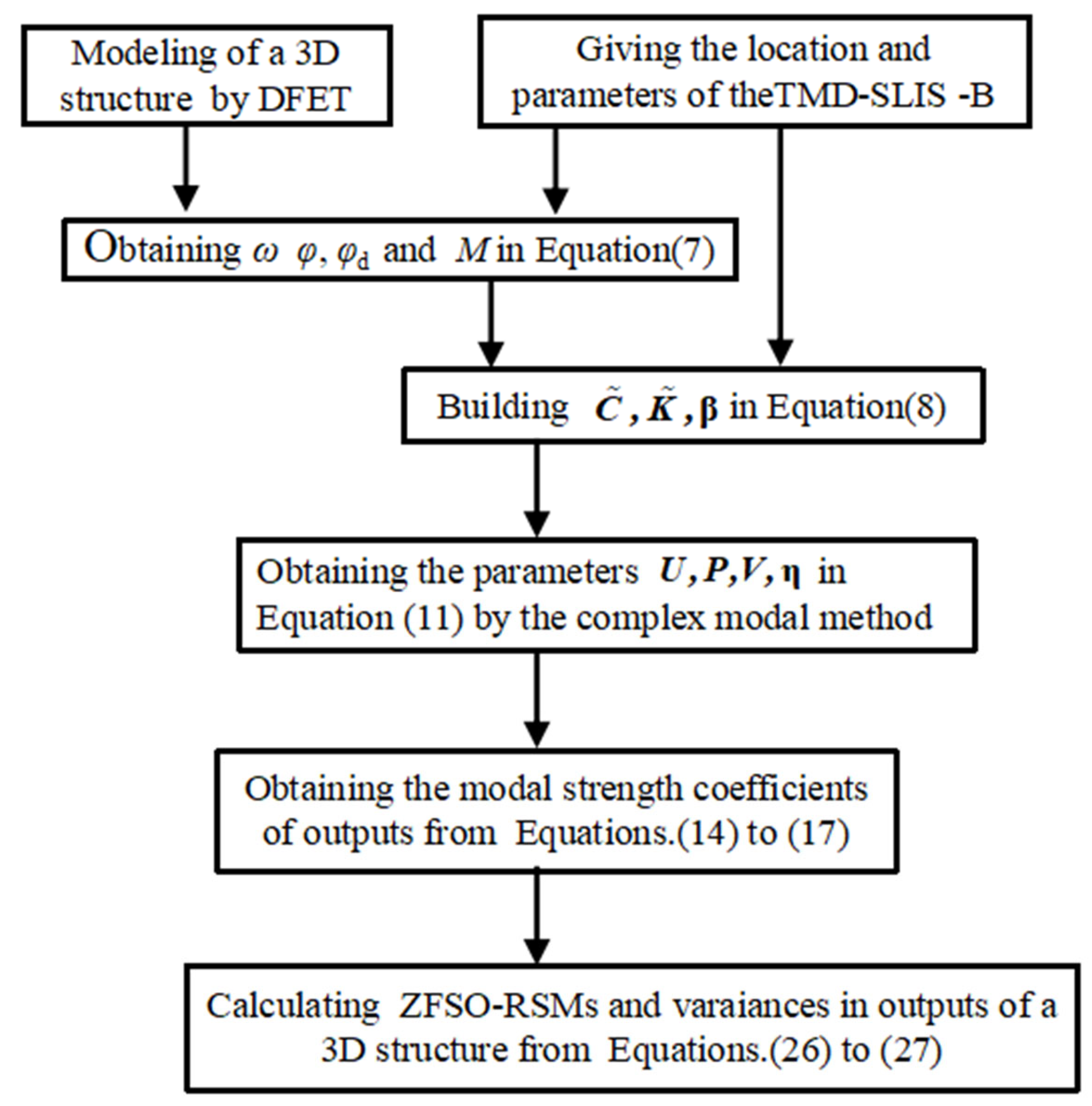
In summary, a method for solving the ZFSO-RSMs and variance in responses is proposed. From Equations (7), (8), and (26), it can be found that the proposed method is free from constraints of the structural form of 3D buildings or the parameters of the TMD-SLIS-B, so the method is general. Figure 4 shows the application flowchart of the proposed method for calculating the ZFSO-RSMs for the seismic response of 3D structures with a TMD-SLIS-B.

4. Optimization of the TMD-SLIS-B’s Parameters Based on Dynamic Reliability

From Figure 2 and Figure 3, a TMD-SLIS-B consists of a TMD, an SLIS, and a bracket with eight mechanical parameters that have different influences on the seismic performance of structures. So, it is important to study the optimum parameters of a TMD-SLIS-B to acquire the biggest mitigation performance or to obtain the most economical damper parameters under the condition of meeting the requirements.

The dimensionless parameter optimization method can be widely applied in engineering research because of its advantages, such as facilitating the simplification of problem analysis, highlighting key factors, and making experimental research and data processing more convenient. In this work, based on the dimensionless method, the expressions of the TMD-SLIS-B’s parameters are [16,25,29]

$$m_{\mathrm{T}}=u_{\mathrm{T}}{m}_s, m_{\mathrm{I}}=u_{\mathrm{T}}{u}_{\mathrm{I}}{m}_s$$

(28a)

$$k_{\mathrm{T}}=u_{{\omega }_{\mathrm{T}}}^2{\omega }_0^2{u}_{\mathrm{T}}{m}_s, k_{\mathrm{I}}=u_{{\omega }_{\mathrm{T}}}^2{u}_{{\omega }_{\mathrm{I}}}^2{\omega }_0^2{u}_{\mathrm{T}}{u}_{\mathrm{I}}{m}_s, k_{\mathrm{B}}=u_{\mathrm{B}}{k}_{\mathrm{T}}$$

(28b)

$$c_{\mathrm{T}}=2u_{{\xi }_{\mathrm{T}}}{\xi }_s{u}_{\omega }^{\mathrm{T}}{\omega }_0{u}_{\mathrm{T}}{m}_s, c_{\mathrm{I}}=2u_{{\xi }_{\mathrm{T}}}{u}_{{\xi }_{\mathrm{I}}}{\xi }_s{u}_{\omega }^{\mathrm{T}}{u}_{{\omega }_{\mathrm{I}}}{u}_{\mathrm{I}}{u}_{\mathrm{T}}{m}_s{\omega }_0, c_{\mathrm{B}}={\xi }_{\mathrm{B}}{k}_{\mathrm{B}}$$

(28c)

where $u_{\mathrm{I}}$ and $u_{\mathrm{T}}$ are the ratio of the SLIS’s coefficient m_I to the TMD’s mass $m_{\mathrm{T}}$ and $m_{\mathrm{T}}$ to the structural overall mass m_s, respectively; $u_{{\omega }_{\mathrm{T}}},u_{{\omega }_{\mathrm{I}}}$ are the ratio of the TMD’s designated angular frequency ${\omega }_{\mathrm{T}}$ to the first natural angular frequency ${\omega }_0$ of the uncontrolled structure and the SLIS’s nominal circular frequency ω_I to ${\omega }_{\mathrm{T}}$, respectively; $u_{{\xi }_{\mathrm{T}}}$ is the ratio of the TMD’s designated damping ratio ${\xi }_{\mathrm{T}}$ to the structural inherent damping ratio ${\xi }_{\mathrm{s}}$ and ${\xi }_{\mathrm{T}}$ to SLIS’s designated damping ratio ${\xi }_{\mathrm{I}}$, respectively; $u_{\mathrm{TB}}$ is the ratio of the bracket’s stiffness k_B to the TMD’s stiffness k_T; and ${\xi }_{\mathrm{B}}$ is the inherent damping ratio. The expressions of ${\omega }_{\mathrm{T}},{\omega }_{\mathrm{I}},{\xi }_{\mathrm{T}},{\xi }_{\mathrm{I}}$ are ${\omega }_{\mathrm{T}}=\sqrt{k_{\mathrm{T}}/m_{\mathrm{T}}},{\omega }_{\mathrm{I}}=\sqrt{k_{\mathrm{I}}/m_{\mathrm{I}}},{\xi }_{\mathrm{T}}=c_{\mathrm{T}}/\left(2\sqrt{k_{\mathrm{T}}{m}_{\mathrm{T}}}\right)$, ${\xi }_{\mathrm{I}}=c_{\mathrm{I}}/\left(2\sqrt{k_{\mathrm{I}}{m}_{\mathrm{I}}}\right)$, respectively.

Three-dimensional structures belong to multi-degree-of-freedom systems with numerous structural dynamic responses, so there are many factors that determine structural safety, such as the displacement and velocity of the vibration of each node. Therefore, when optimizing the parameters of TMD-SLIS-B-equipped 3D structures, it is necessary to find objective functions that include various structural safety factors. The system reliability can comprehensively consider the impacts on structural safety by various response quantities, such as the displacements and velocities of numerous nodes of the structure. It is often regarded as an important parameter for structural safety assessments. Grounded on the first-passage failure criterion, Vanmarcke [34] put forward a theoretical computational formula for dynamic reliability. This formula is characterized by the dual advantages of remarkable precision and high efficiency, and it has been extensively utilized in the evaluation of structural reliability when subjected to random excitation.

As is well known, large mechanical parameters of dampers require large component sizes or complex implementation mechanisms, resulting in higher manufacturing costs of dampers. An optimization method [25,29] is proposed for hybrid damper parameters with the constraints of satisfying the structural system reliability specified in codes and considering the weight of damper parameters. In this work, a TMD-SLIS-B is composed of three parts: a TMD, an inerter, and a bracket. Therefore, it is assumed that the priority levels of the TMD, inerter, and bracket decrease in turn. The priority levels of the eight damper parameters in descending order are as follows: TMD mass, stiffness and damping, inerter coefficient, stiffness and damping of the SLIS, and stiffness and damping of the bracket.

Thus, the optimization method based on system dynamic reliability and considering different weights of the TMD-SLIS-B’s parameters as constraints is expressed as [16,25,29]

$$\mathrm{minimize}\hspace{1em}{\mu }_{\mathrm{T}},{\mu }_{{\omega }_{\mathrm{T}}},{\mu }_{{\xi }_{\mathrm{T}}},{\mu }_{\mathrm{I}},{\mu }_{{\omega }_{\mathrm{I}}},{\mu }_{{\xi }_{\mathrm{I}}},{\mu }_{\mathrm{B}},{\xi }_{\mathrm{B}}$$

(29)

and it is subject to $P_f\le P_{f,\lim }$ and with the weight order ${\mu }_{\mathrm{T}},{\mu }_{{\omega }_{\mathrm{T}}},{\mu }_{{\xi }_{\mathrm{T}}},{\mu }_{\mathrm{I}},{\mu }_{{\omega }_{\mathrm{I}}},{\mu }_{{\xi }_{\mathrm{I}}},{\mu }_{\mathrm{B}},{\xi }_{\mathrm{B}}$, in which $P_f$ and $P_{f,\lim }$ are the system failure probability and its limit, respectively. In this work, the system reliability is evaluated using the weakest failure mode, which takes the maximum value of the failure probabilities of each component. The component failure probability is calculated by Vanmarcke’s method. According to the code [35]), the range of probability indices is 0~1.5, and their corresponding failure probability range is 0.5~0.0668.

For a clear description of the application of the proposed optimization method, an application flowchart by the linear search method is drawn in Figure 5.

5. Numerical Cases

In this section, four cases are employed to sequentially investigate the accuracy of the proposed method for calculating the ZFSO-RSMs of 3D structures with a TMD-SLIS-B, the spatial dynamic characteristics of a 3D structure under a unidirectional seismic load, the effect of the brace’s mechanical parameters in a TMD-SLIS-B on the structural seismic response, and the demonstration of the optimization method for the TMD-SLIS-B’s mechanical parameters. All computations were carried out on an Intel Core i7 processor personal computer with a 2.60 GHz base frequency.

5.1. Basic Information of a 3D Building Structure with a TMD-SLIS-B

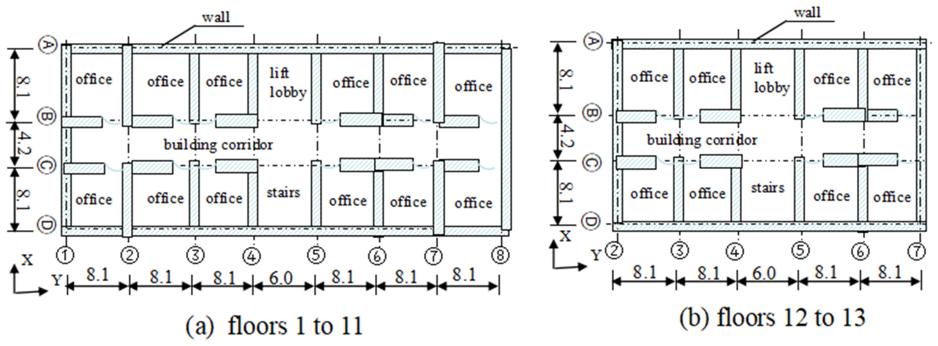
A 13-story steel-reinforced concrete frame structure is used as the main structure for all four numerical examples, and the 3D schematic diagram is shown in Figure 6. The structure has 1 basement floor, 11 floors in part, and the elevator machine room is set on the roof floor. The planar dimensions of the structural beams and columns are shown in Figure 7, in which the dimension units are in meters. The cross-section of the beams does not change with the floor. There are two sizes of beams, namely, B1 and B2, whose specific parameters are shown in

Table 1. Material and section properties of the bare structure.

Section Number of the Structural Member	Young’s Modulus of Elasticity (N/mm2)	Section Type (Width × Height) (mm)
B1	3.25 × 104	Rectangular with 350 × 700
B2	3.25 × 104	Rectangular with 350 × 900
C1	3.25 × 104	Rectangular with 1000 × 1000
C2	3.25 × 104	Rectangular with 800 × 900
C3	3.25 × 104	Rectangular with 700 × 800

. Note that the cross-section of the beam of type B2 is not marked in Figure 7. The height of each floor in the above-ground part of the structure is 3.3 m, and the floor height of the basement floor is 5.1 m. The columns on the same floor adopt the same cross-sectional dimensions, and vertically along the structure, they are divided into two categories, namely, C1 and C2, whose specific parameters are listed in Table 1. A structural elevation layout diagram is shown in Figure 8.

When conducting seismic motion analysis, the lumped mass method is often used to determine the structural mass. According to existing design codes, the lumped mass consists of the self-weight of beams, columns, and floor slabs, the weight of the paving layer of floor slabs, the weight of the walls, and the live load on the floor slabs. Figure 9 shows the building function and wall layout diagram, which is used to calculate the nodal structural mass. In this example, the mass of the beams, columns, and slabs is determined by the structural unit weight and structural dimensions. The floor slab paving is assumed as 1.5 KN/m². The wall load is determined according to the story height and beam height, and it is assumed to be 10 KN/m. The live load of the office is taken as 2.0 KN/m².

To use the structural seismic vibration response analysis method proposed in this manuscript, it is imperative to form a dynamic model by finite element dynamic technology to acquire structural dynamic parameters, i.e., nodal mass, natural circular frequencies, and real mode shapes. In this work, MIDAS Gen [36] was used to acquire these dynamic parameters of the 3D structure. In the numerical example, spatial elements with six degrees of freedom are used to simulate the beams and columns of the building structure. In MIDAS Gen software (2023 version), nodes are positioned at the intersections of structural beams and columns, and the entire 3D structure has a total of 446 nodes. Except for the 32 nodes of the building foundation, the entire structure has a total of 414 nodes. In this article, each node takes into account the dynamic degrees of freedom in two horizontal directions (the X- and Y-directions), and the entire structure has a total of 828 dynamic degrees of freedom. Through modeling and analysis by MIDAS Gen, the concentrated mass of the structural nodes, the natural circular frequencies, and real modal vibration modes of the structure were obtained. According to the research results [25,29], when the number of vibration modes corresponds to the sum of the modal weight reaching 100%, the obtained ZFSO-RSMs of the structural seismic response tend to be stable.

Table 2. The first 42 vibration eigenvalues of the uncontrolled 3D structure.

No. of the Real Modes	Natural Circular Frequency (Rad/s)	Weight of Single Model in X-Direction (%)	Weight of Single Model in Y-Direction (%)	No. of Real Modes	Natural Circular Frequency (rad/s)	Weight of Single Model in X-Direction (%)	Weight of Single Model in Y-Direction (%)
1	3.9669	84.5798	0.0001	22	70.6483	0.0001	0.008
2	4.4291	0.0001	85.703	23	72.5029	0.0024	0.0001
3	4.514	0.0049	0.5626	24	72.8918	0.0001	0.142
4	11.7826	9.9144	0.0001	25	75.7785	0.0679	0.0001
5	13.2135	0.0001	8.7836	26	79.1038	0.0047	0.0001
6	13.4208	0.0021	0.182	27	85.1128	0.0004	0.0209
7	20.5789	2.8901	0.0001	28	85.9527	0.0676	0.0005
8	22.8622	0.0008	2.0326	29	87.4403	0.0001	0.0397
9	23.0605	0.0025	0.5671	30	87.9984	0.0017	0.0002
10	29.6831	1.1924	0.0001	31	89.9784	0.0002	0.003
11	32.4083	0.0040	0.0617	32	96.8567	0.0001	0.0429
12	33.2204	0.0002	0.9586	33	98.6182	0.0078	0.0001
13	40.1307	0.6224	0.0001	34	99.8481	0.0491	0.0001
14	42.7672	0.0017	0.0103	35	105.0883	0.0003	0.0027
15	44.7425	0.0002	0.5077	36	111.2432	0.0001	0.0409
16	52.1133	0.3236	0.0001	37	111.7585	0.0049	0.0001
17	55.5892	0.0002	0.0054	38	115.2953	0.025	0.0001
18	58.0233	0.0001	0.2634	39	118.5760	0.0004	0.0010
19	65.0592	0.1723	0.0001	40	121.5024	0.0006	0.0001
20	66.6247	0.0001	0.0001	41	122.7106	0.0001	0.0017
21	68.9172	0.0022	0.0001	42	123.3887	0.0001	0.0191

shows the first 43 order natural circular frequencies and their modal weights of the vibration modes, whose total weights are 100% in the X-direction and Y-direction, respectively. The total mass m_s of the structure is 1.78 × 10⁷ kg. In addition, the damping ratio in the Rayleigh damping model is assumed as 5%. The seismic motion parameters of Clough–Penzien [37] excitation are assumed as ω_g = 15.72 rad/s, ξ_g = 0.8, ω_f = 8.376 rad/s, ξ_f = 0.8, and S₀ = 0.005777 m²/s³.

5.2. Verifying the Proposed Solutions for ZFSO-RSMs of Dynamic Responses

The PEM [33] is an analytical solution that can accurately obtain the PSDF of the responses of linear structures under random loads. However, the PEM only provides numerical solutions of the ZFSO-RSMs of dynamic responses. In this work, the PEM is used to prove the proposed solutions of the ZFSO-RSMs of the outputs of the 3D structure with a TMD-SLIS-B. Appendix A gives the expressions for the ZFSO-RSMs by the PEM. Comparing Equation (26) with Equation (A16) in Appendix A, both equations are used to calculate the ZFSO-RSMs of the dynamic outputs, but their expressions are significantly different. Here, we must stress that the formulations by the PEM are more complicated, whereas the formulations presented in this paper are comparatively succinct.

According to Equation (8), when analyzing the ZFSO-RSMs and acceleration variances of the structure, the parameters of the TMD-SLIS-B and the real vibration mode parameters need to be given. In the example, the TMD-SLIS-B parameters are assumed as m_T = 0.01 × m_s = 1.78 × 10⁵ kg, m_I = 8.89 × 10⁴ kg, k_T = 1.79 × 10⁶ N/m, k_I = 1.14 × 10⁶ N/m, k_b = 10 × k_T = 1.78 × 10⁷ N/m, c_T = 1.78 × 10⁵ N s/m, c_I = 6.34 × 10⁴ N s/m, and c_B = 0.01k_b = 6.55 × 10⁴ N s/m, and 42 models are taken. The TMD-SLIS-B is assumed to be installed at the intersection of Axis-4 and Axis-C on the structural roof. In addition, with regard to Equation (7a) and Table 2, when analyzing the ZFSO-RSMs of the responses of a 3D structure with a TMD-SLIS-B, the quantity of real modal shapes of the uncontrolled structure is selected as 42 in this case.

From Equation (A16) in Appendix A, the calculation accuracy using the PEM is related to the numerical integration step Δω and the upper integration limit ω_u. Through iterative trials, ω_u = 1000 rad/s is found to give a highly accurate numerical solution. In order to reveal that the calculation method for ZFSO-RSMs proposed in this work is closed-form, the three integration intervals are chosen as three cases: 0.5rad/s, 0.05 rad/s, and 0.005 rad/s.

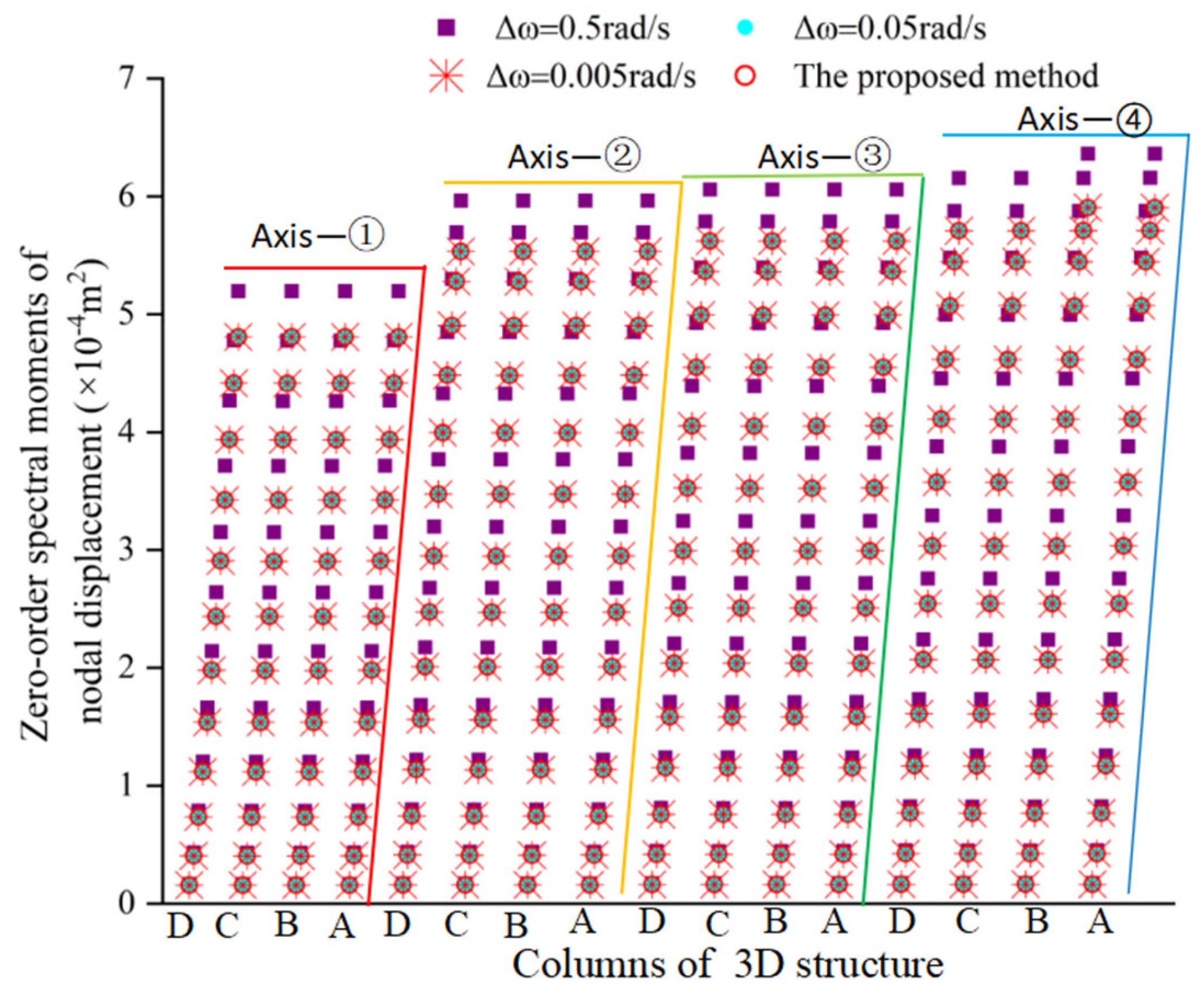
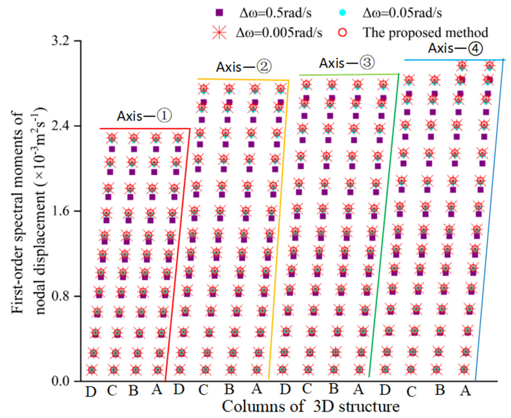
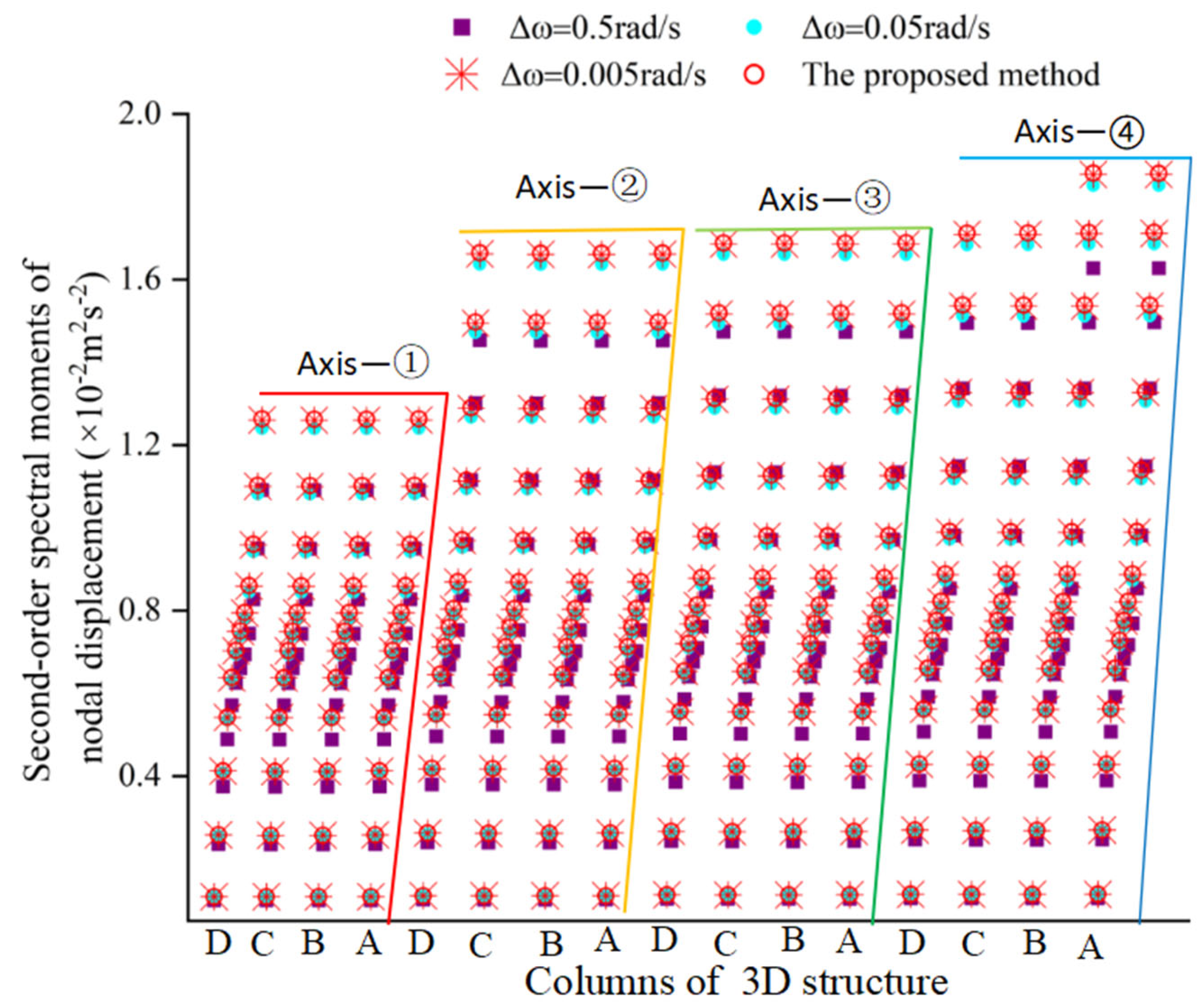
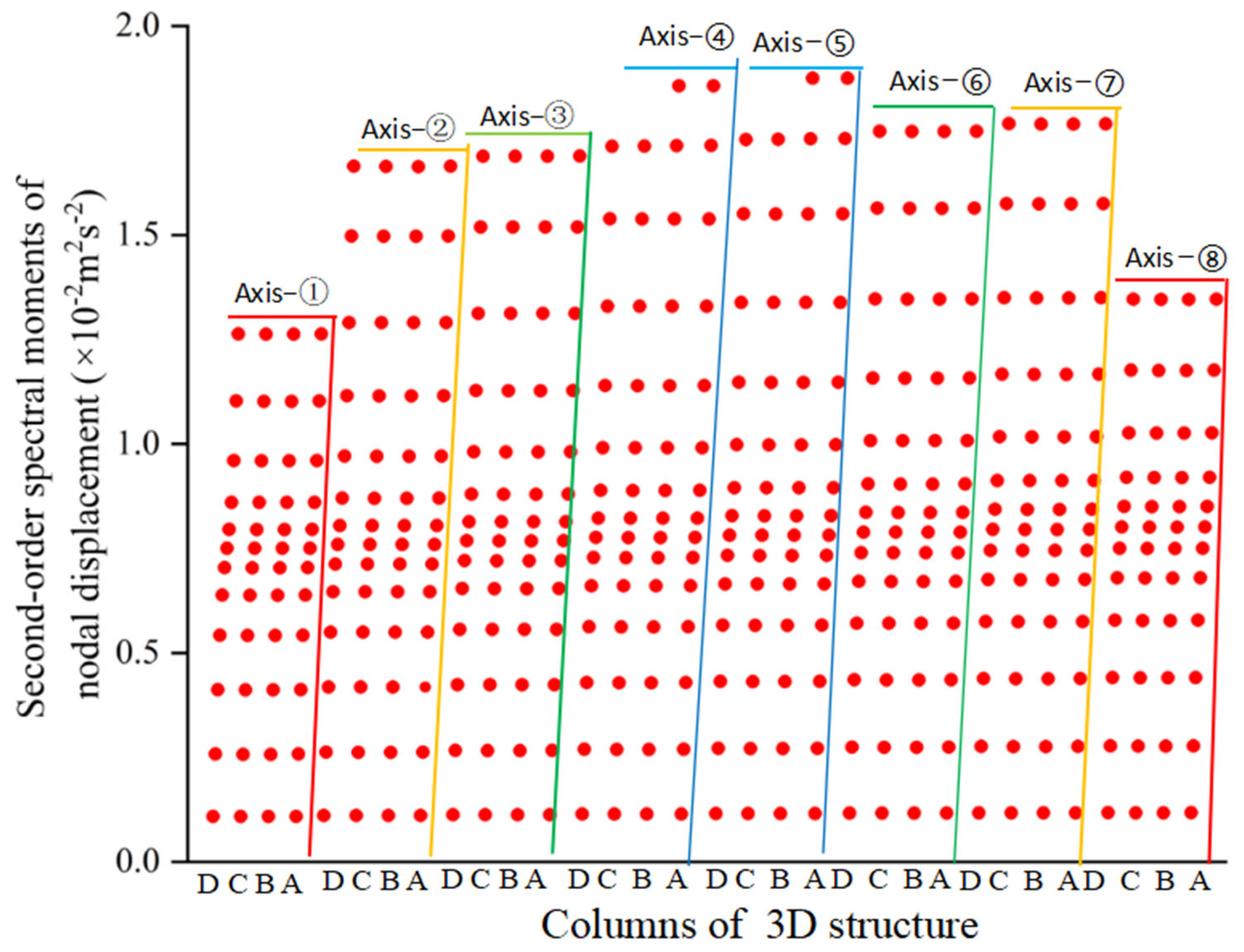
Figure 10,Figure 11 and Figure 12, respectively, show the zero-order to second-order spectral moments of the nodal displacements of Axes 1 to 4 calculated by the PEM and the proposed method.

Table 3. Comparison of inter-story deformation and responses of components in the TMD-SLIS-B calculated results by the PEM and the proposed method.

Items	Zero-Order Spectral Moment		First-Order Spectral Moment		Second-Order Spectral Moment
	Δω = 0.005 Rad/s by the PEM	The Proposed Method	Δω = 0.005 Rad/s by the PEM	The Proposed Method	Δω = 0.005 Rad/s by the PEM	The Proposed Method
the second floor of the column at the intersection of Axis-A and Axis-①	5.876 × 10−6 m2	5.876 × 10−6 m2	3.683 × 10−5 m2s−1	3.686 × 10−5 m2s−1	3.378 × 10−4 m2s−2	3.382 × 10−4 m2s−2
xB	5.478 × 10−7 m2	5.478 × 10−7 m2	2.632 × 10−6 m2s−1	2.634 × 10−6 m2s−1	1.671 × 10−5 m2s−2	1.674 × 10−5 m2s−2
FI	1.758 × 108 N2	1.758 × 108 N2	8.471 × 108 N2s−1	8.480 × 108 N2s−1	5.420 × 109 N2s−2	5.429 × 109 N2s−2
xT	2.661 × 10−3 m2	2.661 × 10−3 m2	1.063 × 10−2 m2s−1	1.1061 × 10−2 m2s−1	4.622 × 10−2 m2s−2	4.611 × 10−2 m2s−2

lists the ZFSO-RSMs, the inter-story deformation of the second floor of the column at the intersection of Axes-A and Axes-①, the TMD’s deformation, the SLIS’s force, and the brace’s deformations in the case of Δω = 0.005 rad/s.

From Figure 10, Figure 11 and Figure 12 and Table 3, it is concluded that the PEM-based computation results stabilize as the integration step size decreases and exactly match the proposed method when the step size equals 0.005 rad/s. In addition, the ZFSO-RSMs of the nodes on the same floor are nearly identical, which confirms the assumption of infinite in-plane stiffness for the planar frame structure. So, the nodal absolute displacements of a column can represent the absolute displacement of the whole structure in the example.

From Equations (26) and (27), it can be found that the spectral moment of a certain response is represented as a linear combination of formulas governed by the complex vibration eigenvalues, the modal spectral moment, and the modal intensity coefficient of the EDS. In this calculation example, a total of 5241 response values were calculated, including the ZFSO-RSMs and acceleration variances in the absolute displacements of 436 nodes in the X-direction and Y-direction, the inter-story displacements of 436 stories in the X-direction and Y-direction, the TMD’s displacements, the SLIS’s force, and the brace’s deformation. When using the presented method for calculating these values, the time consumption was 1.06 s, while the time consumption of the PEM (Δω = 0.005rad/s), which is consistent with the calculation results of this paper, was 514.195 s. In practical engineering, when only a small number of structural dynamic responses determine the safety assessment of structures, the method proposed in this manuscript can be used for the stochastic seismic response analysis and safety assessment of large-scale complex structures, and it has high analysis efficiency.

5.3. Spatial Dynamic Properties for 3D Structures Under Unidirectional Seismic Excitation

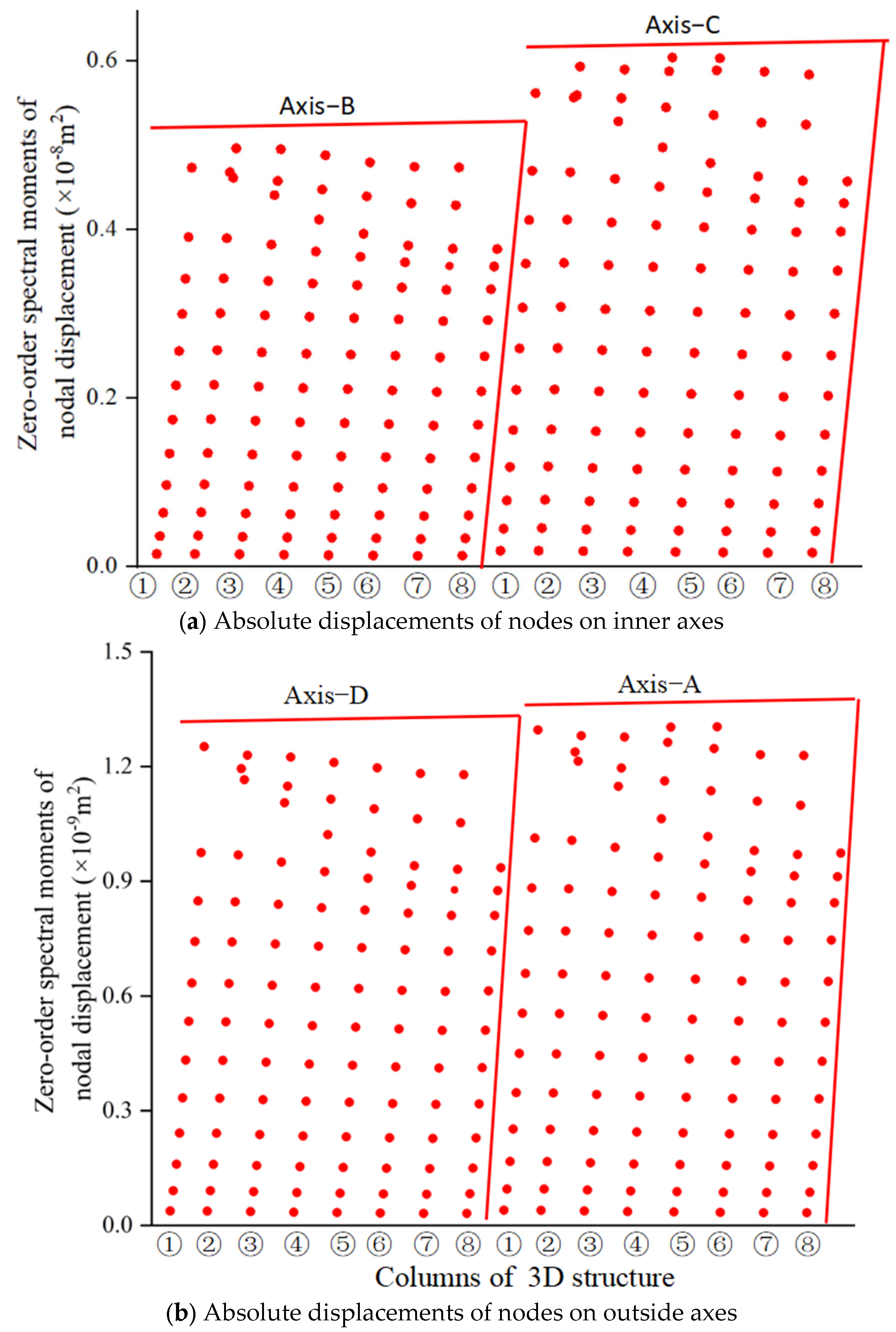
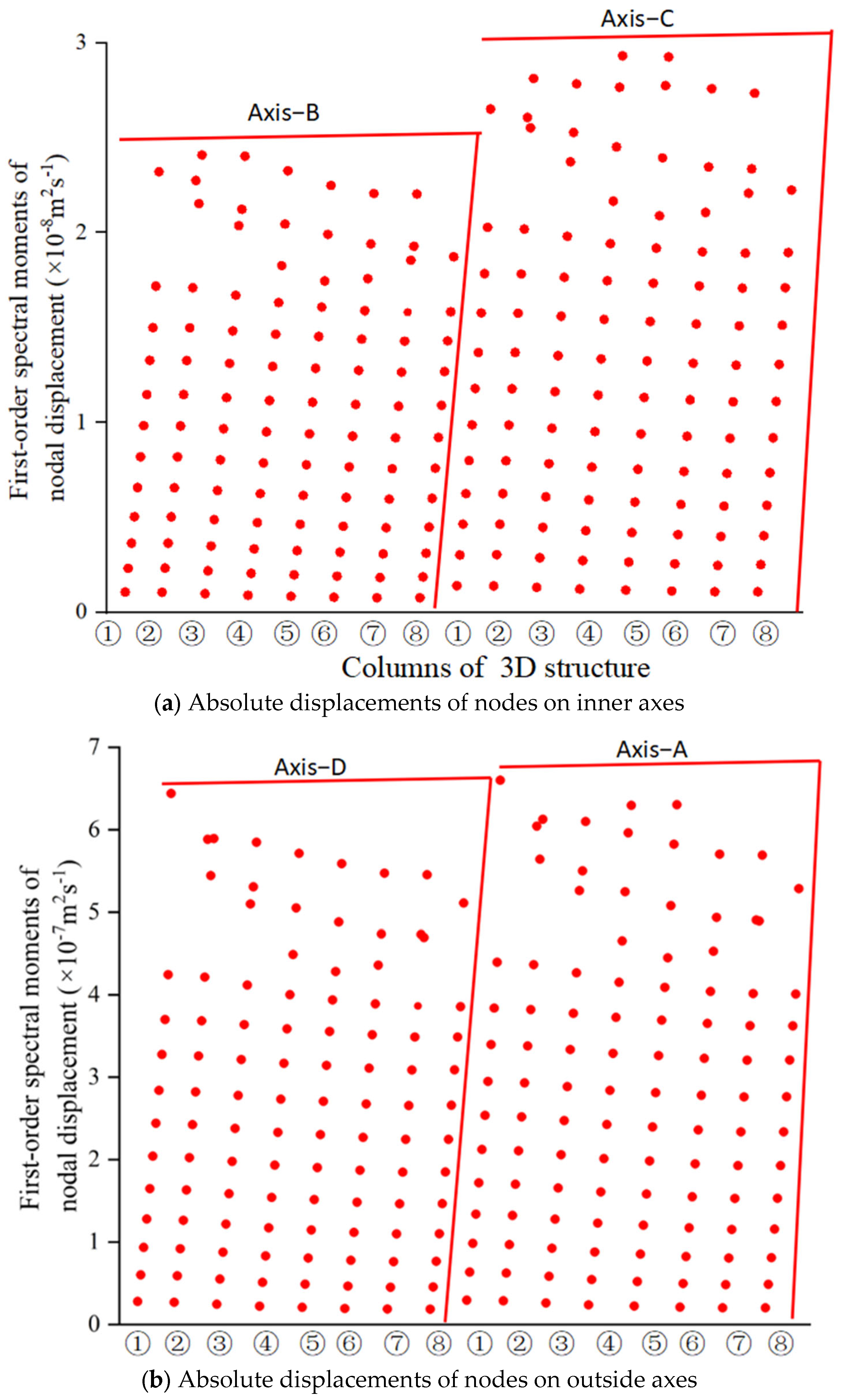
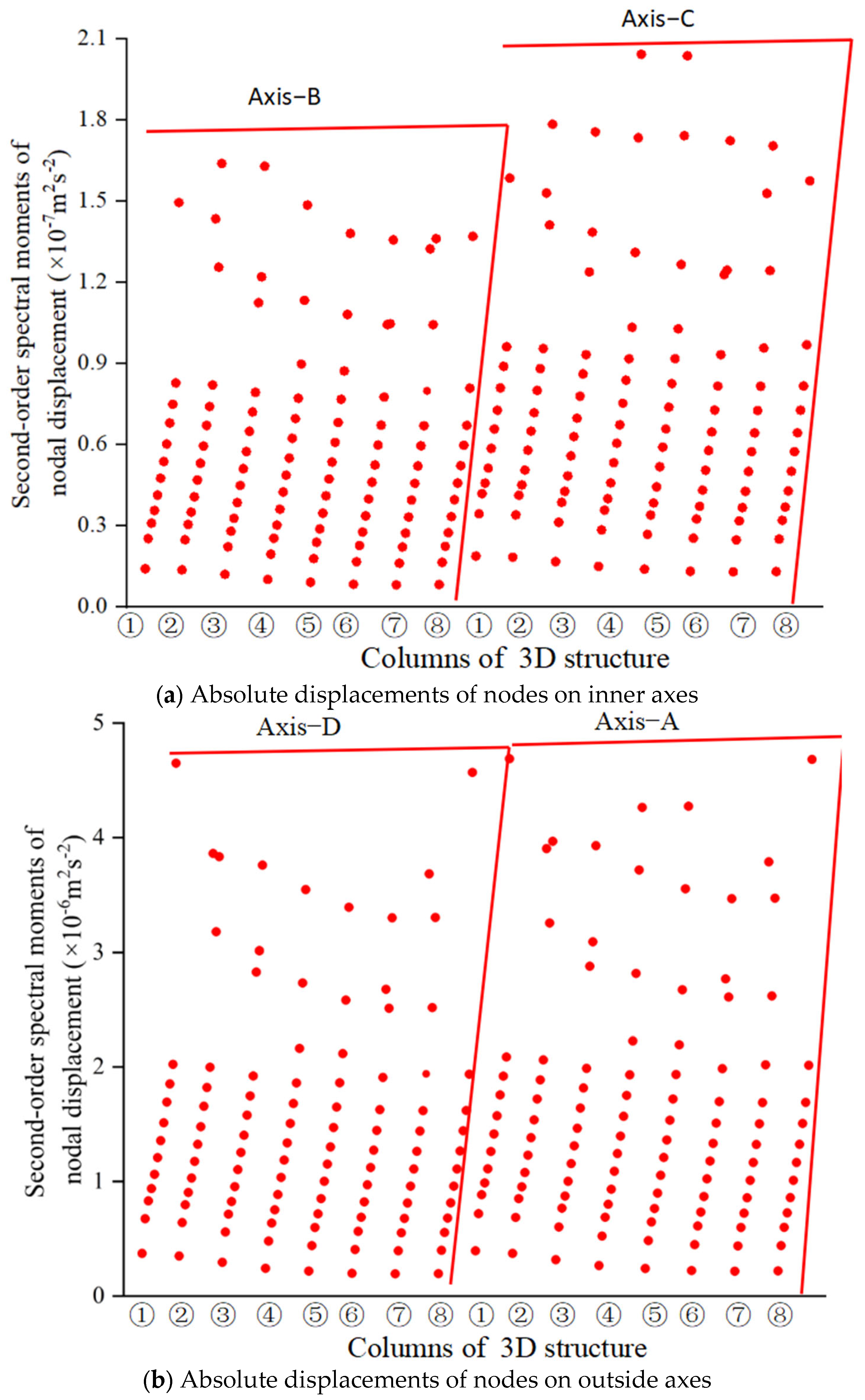
To systematically study the spatial properties of the structural dynamic response subjected to random seismic loads, a specific comparative analysis scheme is selected as the zero-order, first-order, and second-order spectral moments of the nodal absolute X-direction and Y-direction displacements of the 3D structure, as shown in Figure 13, Figure 14, Figure 15, Figure 16, Figure 17 and Figure 18. It should be noted that each column of data in Figure 13, Figure 14, Figure 15, Figure 16, Figure 17 and Figure 18 represents the response spectral moments of the nodes at each floor of a column. In Figure 13, Figure 14 and Figure 15 the columns are sorted by the X-direction first and then the Y-direction, while in Figure 16, Figure 17 and Figure 18 the sorting order is the Y-direction responses first and then the X-direction responses. Additionally, the parameters and setting location of the TMD-SLIS-B in the example are the same as those in Section 5.2.

As shown in Figure 13, Figure 14 and Figure 15 the ZFSO-RSMs of the nodal X-direction displacements of the four columns on the same floor on the same numerical axis (e.g., Axis−①) are almost identical, so the spectral moments of one column can be used to replace those of all columns on the same numerical axis. From Axis−① to Axis−⑧, the nodal spectral moments on the same floor exhibit a slight gradual decrease. Here, it should be noted that since the damper TMD-SLIS-B is installed on Axis−④, it indicates that the damper’s installation position is asymmetric and closer to the side of Axis−①. This might be the reason why the structural displacement response spectral moments gradually increase from Axis−① to Axis−⑧.

To verify the difference, the ZFSO-RSMs of the X-direction displacements for nodes in the columns on Axis−① and Axis−⑧ were compared. The max ratios of the former to the latter are 1.06, 1.05, and 1.03, respectively, and such deviations are negligible in engineering. Therefore, the X−direction motion of the 3D structure is considered to satisfy the assumption of infinite in-plane stiffness, meaning that the spectral moments of one column along the X−direction can be used to replace those of the entire 3D structure in the X−direction.

As seen from Figure 16, Figure 17 and Figure 18 for the 3D structure, the ZFSO-RSMs of the nodal displacements in the Y−direction between the inner axes (Axis−B and Axis−C) and the outer axes (Axis−A and Axis−D) differ by at least 10 times, with the former being much smaller than the latter. In addition, the ZFSO-RSMs of the displacement of each node on the same floor of the same letter−axis (e.g., A-axis) have obvious differences, especially those on the 12th floor. This phenomenon may be caused by the installation of the TMD-SLIS-B on the 12th floor and the asymmetry of its location. Therefore, it is necessary to use a spatial structure model to investigate the seismic responses in the Y−direction for a 3D structure with a TMD-SLIS-B.

By comparing the zero-order spectral moments (shown in Figure 12 and Figure 15), the first-order spectral moments (shown in Figure 13 and Figure 16), and the second−order spectral moments (shown in Figure 14 and Figure 17) of the X−direction and Y−direction seismic responses of the 3D structure, it is found that the X-direction response values of the structure are approximately 10⁴ times that of the Y−direction responses. This is because the earthquake ground motion excitation studied in this paper is applied along the X−direction. In this regard, the spatial effect of the structure is not very obvious.

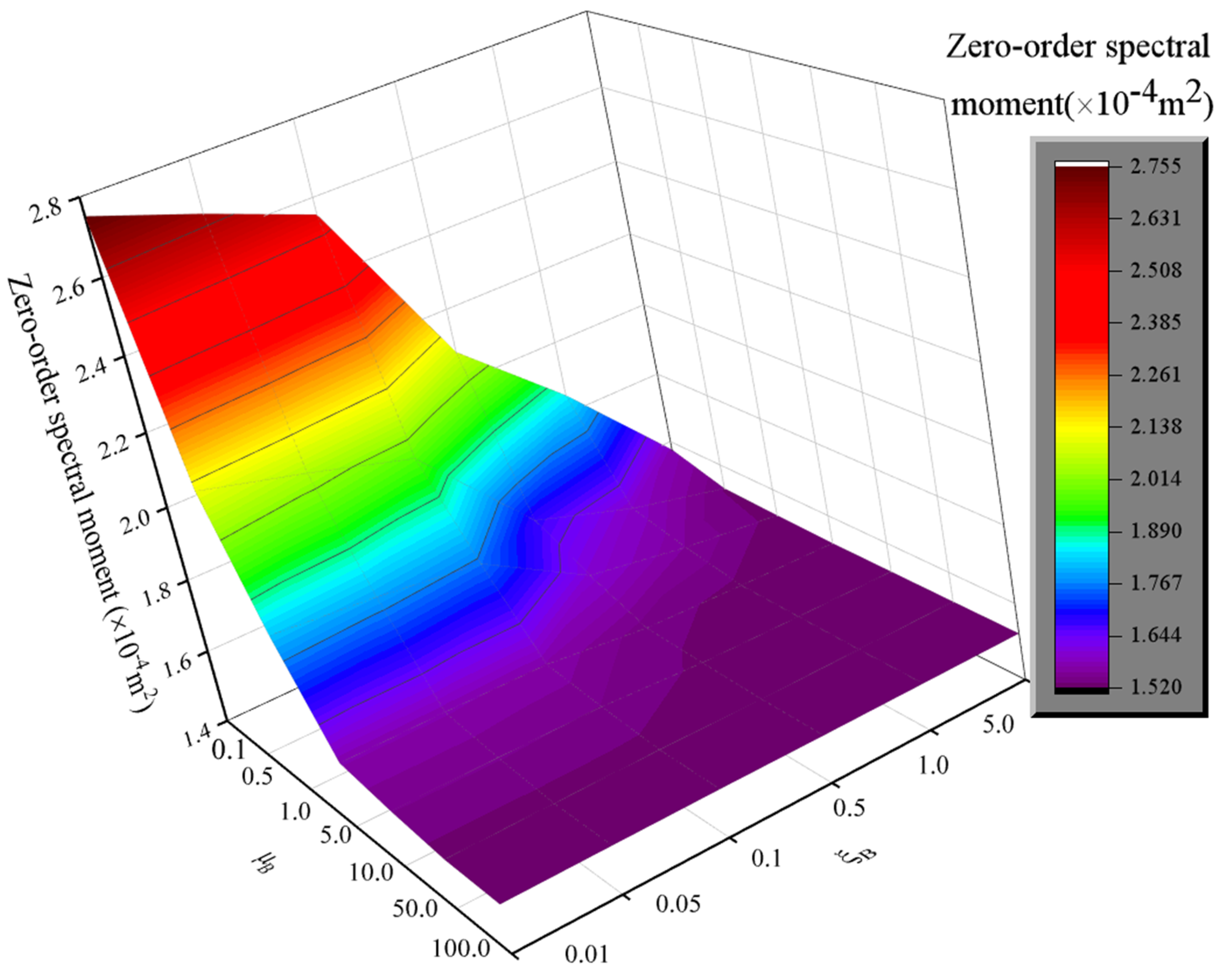
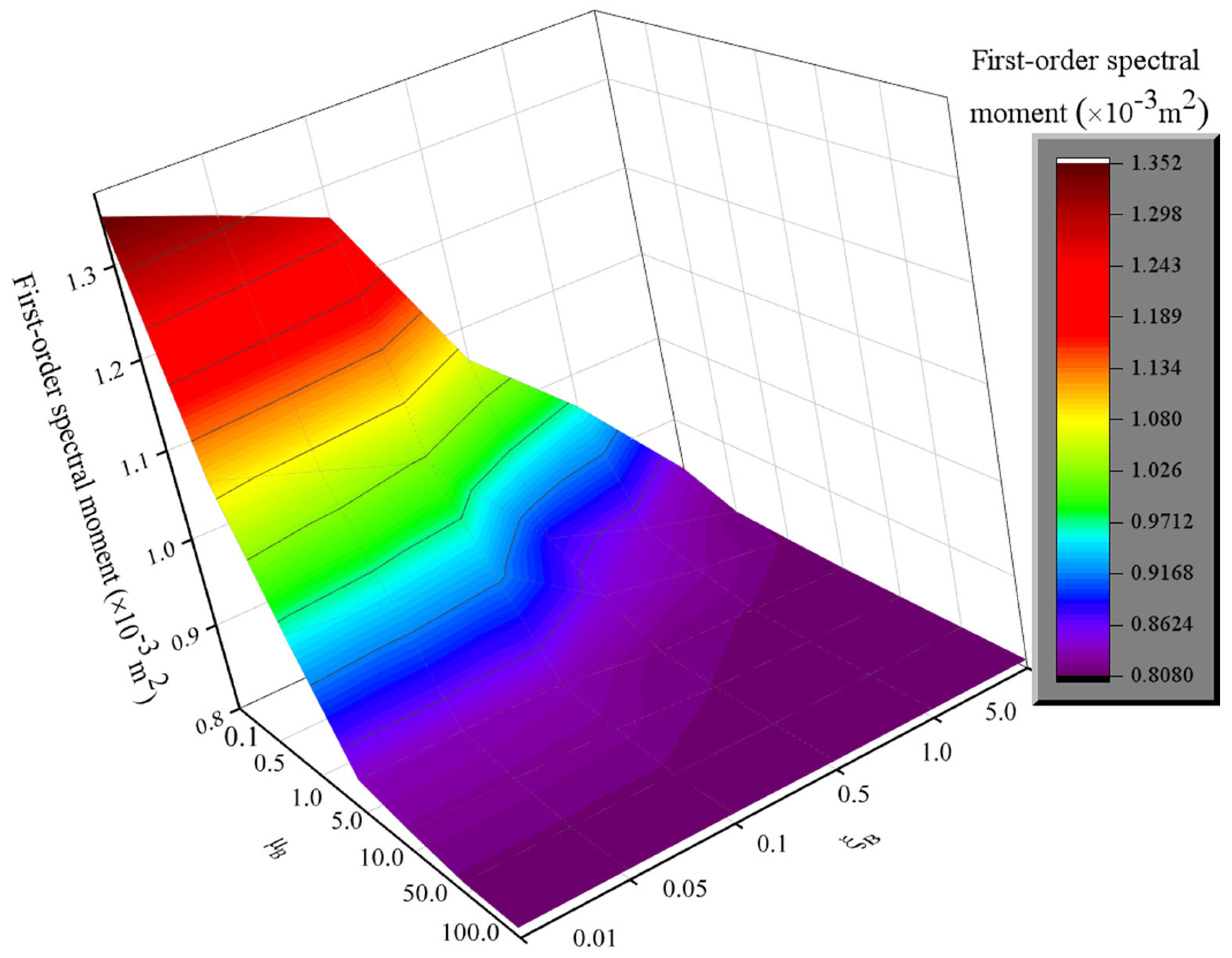
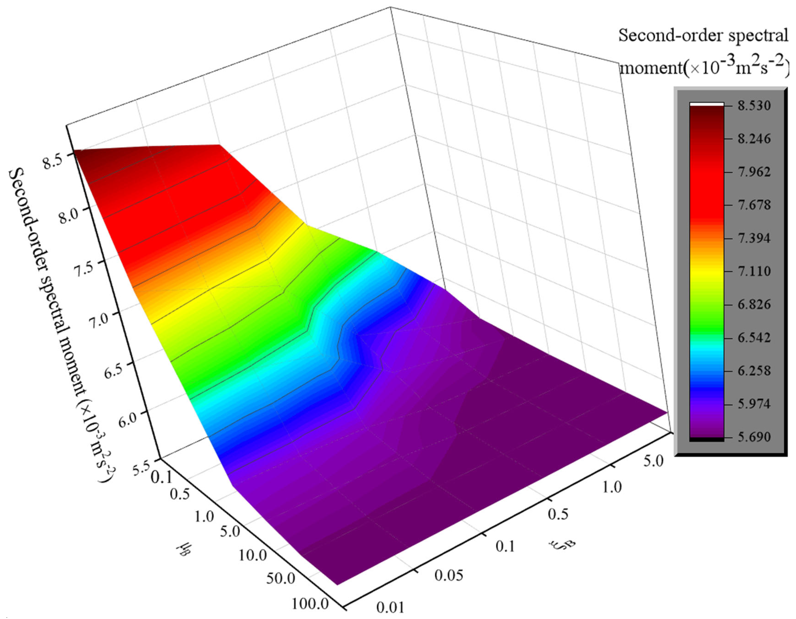
5.4. Influence of the Bracket’s Mechanical Parameters in a TMD-SLIS-B on the Structural Response

A TMD-SLIS-B is composed of a TMD, an SLIS, and a bracket in series. The bracket serves to connect the SLIS and the TMD to the main building structure. Since the bracket is in series with the SLIS, the magnitudes of its stiffness and damping parameters will affect the energy-absorption capabilities of the SLIS and the TMD, thus influencing the shock mitigation efficiency of the entire hybrid damper. In this work, the ZFSO-RSMs of the X-direction nodal displacement are selected as the key evaluation indicators to deeply study the influence of the bracket’s parameters on the vibration reduction effect of the hybrid damper.

According to the relationship of the bracket’s parameters (e.g., $k_{\mathrm{B}}=u_{\mathrm{B}}{k}_{\mathrm{T}}$, $c_{\mathrm{B}}={\xi }_{\mathrm{B}}{k}_{\mathrm{B}}$) established in Section 4, the effect of the bracket’s mechanical parameters on the seismic reduction in the 3D structure is studied by changing u_B and ${\xi }_{\mathrm{B}}$. In addition, as can be seen from the content of Section 5.3, the ZFSO-RSMs of the nodal X-direction displacements of one column can replace those of the entire structure. Therefore, Figure 19, Figure 20, Figure 21 and Figure 22 depict the relationship between the bracket’s parameters and the ZFSO-RSMs of the nodal displacements of the column at the intersection of Axis-① and Axis-A. In the example, u_B values are selected as 0.1, 0.5, 1.0, 5.0, 10.0, 50.0, and 100.0, and ${\xi }_{\mathrm{B}}$ values are selected as 0.01, 0.05, 0.1, 0.5, and 5.0. In addition, except for the bracket’s parameters, the other parameters and location of the TMD-SPIS-B are consistent with those in Section 5.2.

As the bracket parameters gradually increase with the dimensionless parameters u_B and ${\xi }_{\mathrm{B}}$, the mechanical parameters of the bracket also increase. It can be seen from Figure 19, Figure 20 and Figure 21 that the displacement spectral moments in the X-direction of the 3D structure with dampers gradually decrease as the dimensionless parameters increase. The influence of u_B is more significant, while the influence of ${\xi }_{\mathrm{B}}$ is less pronounced. When u_B reaches a certain value, the damping effect of the TMD-SLIS-B tends to stabilize. This indicates that once the bracket’s stiffness reaches a certain level, further changes have minimal impact on the damper’s effectiveness. A higher stiffness of the bracket implies increased material usage and higher costs, which is undesirable in engineering. Therefore, the bracket parameters significantly affect the damping performance of the structure with dampers, necessitating optimization analysis.

5.5. Optimization Analysis of the TMD-SLIS-B’s Parameters Based on Dynamic Reliability

An example is carried out to illustrate the application of the presented method to optimize the TMD-SLIS-B’s parameters. In the example, the key parameters are as follows: the reliability index is 1.0, and its corresponding $P_{f,\lim }$ is 0.1587; 12 inter-story deformations of the column at the intersection of Axis-4 and Axis-C are used as indicators; the limit of the inter-story deformation of linear structures is h/550, where h is the inter-story height; and the time-consuming vibration history T_r is 15s. Based on the flowchart shown in Figure 5, the linear search method is applied to find the TMD-SLIS-B’s optimal parameters. The eight parameters are assumed as follows: 0.01 ≤ u_T ≤ 0.2, with Δu_T = 0.01, 0.5 ≤ u_ωT ≤ 1.2, with Δu_ωI = 0.1, 0.5 ≤ u_ξT ≤ 2.0, with Δu_ξT = 0.5, 0.4 ≤ u_I ≤ 1.0, with Δu_I = 0.1, 0.1 ≤ u_ωI ≤ 0.5, with Δu_ωI = 0.1, and 0.5 ≤ u_ξI ≤ 2.0, with Δu_ξI = 0.5. u_B is selected from the values 0.1, 0.5, 1.0, 5.0, and 10.0, and ξ_B is selected from the values 0.01, 0.05, and 0.1.

Using the proposed optimization method, the optimized parameters are obtained as follows: ${\mu }_{\mathrm{T}}=0.05,{\mu }_{{\omega }_{\mathrm{T}}}=0.9,{\mu }_{{\xi }_{\mathrm{T}}}=2.0,{\mu }_{\mathrm{I}}=0.4,{\mu }_{{\omega }_{\mathrm{I}}}=0.4,{\mu }_{{\xi }_{\mathrm{I}}}=1.5,{\mu }_{\mathrm{B}}=1.0,{\xi }_{\mathrm{B}}=0.1$. With regards to the shock absorption effect, based on these optimized parameters, the system failure probability for the 3D structure is 0.1587, while that of the bare structure is 0.949. Figure 22 shows the reduction rates of the zero-order spectral moments (Zero-OSMs), the first-order spectral moments (First-OSMs), and the second-order spectral moments (Second-OSMs) of the absolute displacements and inter-story displacement of the column at the intersection of Axis-① and Axis-A compared with those of the bare structure.

As shown in Figure 22, the reduction ratios of the ZFSO-RSMs of the absolute displacements and inter-story displacements of the floors first increase and then decrease with the floors. Among them, the reduction ratios of the absolute displacements reach a maximum at the 10th floor, while those of the inter-story displacements reach a maximum at the 4th floor. Under the condition of the TMD-SLIS-B’s optimal parameters, the shock absorption effect of the TMD-SLIS-B on the ZFSO-RSMs of the structural absolute displacements and inter-story displacements gradually decrease. This indicates that the TMD-SLIS-B can effectively reduce the absolute displacements and inter-story displacements of a 3D structure; however, it exhibits a better shock absorption effect for absolute displacements. Therefore, TMD-SLIS-Bs specified with suitable parameters are effective in enhancing the dynamic reliability of damped 3D structures.

6. Conclusions

Simple analytical solutions for the ZFSO-RSMs of a 3D structure with a TMD-SLIS-B under Clough–Penzien excitation were deduced, and based on the proposed solutions, the spatial dynamic characteristics of a 3D building subjected to unidirectional seismic stationary excitation, the influence of mechanical parameters of a bracket in a TMD-SLIS-B on the structural response, and an optimal method for TMD-SLIS-B’s parameters was also proposed. The key discoveries are presented below:

(1)

The coupled dynamic equations for 3D structures with a TMD-SLIS-B are first proposed, using the principles of TMD-SLIS-B mechanics and D’Alembert’s dynamics theory. The DFET is applied to effortlessly obtain the real-mode vibration parameters of a bare 3D structure to form coupled equivalent seismic motion equations. The establishment of the equivalent equations of a 3D structure with a TMD-SLIS-B can solve the challenge that the stiffness matrix and damping matrix in the 3D structural dynamic equation are not easy to obtain by existing methods. Therefore, the proposed method for the coupled dynamic equations is unrestricted by real 3D structural sophistication.

(2)

By applying the QD-PSDF, simple analytical solutions to the ZFSO-RSMs of the multiple responses of 3D structures with a TMD-SLIS-B under Clough–Penzien excitation are proposed. Compared with the PEM, the presented analytical solutions are simple, and the calculation time of the proposed method is approximately 1/500 of that of the PEM in Case 1. And it can also be used in roll-out analysis of the dynamic outputs of linear structures under other stationary random excitations.

(3)

Using the proposed analytical solutions for the ZFSO-RSMs, the spatial dynamic characteristics of the 3D structure with a TMD-SLIS-B under unidirectional seismic excitation (X-direction) were studied. The results (as shown in Figure 13, Figure 14, Figure 15, Figure 16, Figure 17 and Figure 18) show that the X-direction motion (along the earthquake motion vibration) of the 3D structure can be considered to satisfy the assumption of infinite in-plane stiffness. However, the absolute displacements in the Y-direction (perpendicular to the earthquake motion) of the columns on the outer axes are significantly larger than those of the inner axes, failing to satisfy the plane section assumption. Additionally, the Y-direction responses are much smaller than those in the X-direction and can be neglected. From this perspective, the spatial effect in this case study is not very significant, possibly because of the symmetrical nature of the main structure. However, the direction of ground motion is random and spatial, and it cannot be confined to the principal axes of the building. Moreover, the building itself may not be a symmetric structure. Therefore, future research will investigate the spatial effects of asymmetric structures under unidirectional and three-dimensional spatial excitation. In addition, the damage to building structures during strong earthquakes exhibits typical nonlinear characteristics. It is also necessary to conduct research on the spatial effects of nonlinear structures under random excitation.

(4)

Using the proposed analytical solutions for the ZFSO-RSMs, the influence of the parameters of the bracket in the TMD-SLIS-B on the vibration reduction performance of absolute displacements in the direction of earthquake vibrations was investigated. The results (as shown in Figure 19, Figure 20 and Figure 21) showed that the bracket’s parameters significantly affect vibration reduction performance of the structure with a TMD-SLIS-B, wherein the influence of the bracket’s stiffness is more significant than that of the bracket’s damping. However, when the bracket’s parameter values reach a certain level, their influence on the damping efficiency of the damper tends to stabilize.

(5)

The implementation difficulty for each component of the damper determines the cost of the damper. This manuscript proposes a TMD-SLIS-B parameter optimization method taking the parameter weights determined by the economic efficiency of damper components and the system dynamic reliability as constraint conditions. The case study shows that the presented approach can offer a solution for the real-world engineering application of cost-effective damper settings on structures described by MDOF structures.