A Small-Sample Prediction Model for Ground Surface Settlement in Shield Tunneling Based on Adjacent-Ring Graph Convolutional Networks (GCN-SSPM)

Abstract

In some projects, a lack of data causes problems for presenting an accurate prediction model for surface settlement caused by shield tunneling. Existing models often rely on large volumes of data and struggle to maintain accuracy and reliability in shield tunneling. In particular, the spatial dependency between adjacent rings is overlooked. To address these limitations, this study presents a small-sample prediction framework for settlement induced by shield tunneling, using an adjacent-ring graph convolutional network (GCN-SSPM). Gaussian smoothing, empirical mode decomposition (EMD), and principal component analysis (PCA) are integrated into the model, which incorporates spatial topological priors by constructing a ring-based adjacency graph to extract essential features. A dynamic ensemble strategy is further employed to enhance robustness across layered geological conditions. Monitoring data from the Wuhan Metro project is used to demonstrate that GCN-SSPM yields accurate and stable predictions, particularly in zones facing abrupt settlement shifts. Compared to LSTM+GRU+Attention and XGBoost, the proposed model reduces RMSE by over 90% (LSTM) and 75% (XGBoost), respectively, while achieving an R² of about 0.71. Notably, the ensemble assigns over 70% of predictive weight to GCN-SSPM in disturbance-sensitive zones, emphasizing its effectiveness in capturing spatially coupled and nonlinear settlement behavior. The prediction error remains within ±1.2 mm, indicating strong potential for practical applications in intelligent construction and early risk mitigation in complex geological conditions.

1. Introduction

With the rapid expansion of urban development, shield tunneling has become a preferred method for underground construction, because of its efficiency in advancing tunnels and low disturbance to surrounding structures. When advancing the tunnel, surface settlement remains a persistent engineering challenge during excavation, driven by factors such as stress redistribution, soil heterogeneity, and groundwater variation. Moreover, excessive settlement can jeopardize tunnel integrity, induce structural deformation in adjacent buildings, and damage underground utilities. Recent studies have also demonstrated that dynamic disturbances may intensify the damage to buildings and lead to destruction, particularly in sensitive concrete structures [1]. Therefore, the accurate prediction of surface settlement is crucial for achieving intelligent excavation and implementing effective risk mitigation strategies in shield tunneling projects [2].

Traditional approaches in predicting surface settlement caused by shield tunneling rely on empirical models and numerical simulations. These methods focus on theoretical derivation based on soil properties and tunnel geometry, which results in a huge workload in collecting data. Recent studies have shifted toward data-driven strategies that model the implicit relationship between ring advancement and surface deformation due to technological development. This study adopts a mapping task between shield ring sequences and monitored settlement, using a graph-based framework to capture spatial dependencies among adjacent rings.

The mapping enables engineers to better understand disturbance propagation during excavation, characterizing the disturbance patterns induced by excavation and tracing their propagation through heterogeneous subsurface layers [3,4]. Present studies aim to find the key influencing factors of shield-induced settlement using a graph-based structural method, improving predictive accuracy and interpretability under complex urban geological conditions. However, existing models predominantly rely on large datasets and sequential learning methods [5,6]. Such approaches often fail to capture the spatial dependencies among adjacent rings, resulting in uncertainty in settlement, particularly in small-sample or geologically variable projects [7].

Recent advancement in graph neural networks (GNNs) and small-sample learning create more applicable approaches to settlement prediction in shield tunneling projects [8]. Surface settlement is not solely governed by construction parameters but also by the spatial coupling and interaction among shield rings [9]. GNNs have the capability to extract meaningful factors from multiple datasets and model topological spatial relationships that drive settlement [10,11,12]. Existing research has further integrated GNNs with techniques that extract features across multiple scales to enhance the performance of shield-induced settlement prediction models, demonstrating reliable results [13,14].

Deep learning technologies have contributed to the study of settlement prediction in underground construction by offering enhanced feature extraction and nonlinear mapping capabilities [15]. CNNs and LSTMs have been used to analyze settlement sequences, identifying the trends and abrupt changes [16]. Moreover, the main focus has turned to integrating explainable models with GNNs to investigate the spatial disturbance mechanisms inherent in shield tunneling [17,18]. GCN-based methods have shown the ability to identify local abrupt settlement zones even when monitoring data are limited [19]. A model that predicts the impact of the cutter-head based on the parameters of the machine is proposedto investigate the ground behavior caused by the cutter-head [20]. An effective prediction of surface settlement during shield tunneling provides information on the ground response and enables a timely adjustment of shield operating parameters to ensure excavation stability [21]. Geotechnical investigations indicate that settlement has a spatially continuous manner with layered response characteristics [22]. This behavior is caused by a complex interaction of factors of the soil which collectively create a nonlinear, multilevel coupling system extending from shallow to deep layers [23]. In the process of shield tunneling, the disturbance between adjacent rings forms the physical basis for spatial correlation in settlement evolution [24]. Although several studies have used graph-based frameworks to simulate this propagation mechanism [25], most of them lack a comprehensive representation of the hierarchical structure and fail to adequately capture dynamic transmission across multiple rings. These studies affirm the feasibility and adaptability of graph-based and spatially aware models. Moreover, deep learning has been applied to predict the surface settlement to address gaps in field observations. Such advancements mark a shift away from traditional data heavy models and emphasize the growing importance of intelligent modeling in the initial planning, construction monitoring, and post-construction assessment of urban tunneling projects.

This study develops a novel small-sample prediction framework based on adjacent-ring graph convolutional networks (GCN-SSPM). The model leverages the physical adjacency among shield rings to construct a chain-like graph structure that captures spatial disturbance propagation during tunnel advancement. By stacking multiple graph convolution layers, the network aggregates neighborhood information across successive rings, enhancing its capacity to model localized settlement responses in complex geological settings. During the data preparation phase, Gaussian-weighted smoothing is applied to mitigate high-frequency noise, while empirical mode decomposition (EMD) is used to extract intrinsic mode functions (IMFs) that reflect multi-scale temporal features. These are then combined with lagged settlement structures and reduced via principal component analysis (PCA) to construct a compact and informative input tensor that integrates both temporal memory and frequency-domain characteristics. To improve generalization across varying settlement zones, a dynamic ensemble strategy is further introduced. This mechanism dynamically integrates predictions from GCN-SSPM, LSTM+GRU+Attention, and XGBoost by assigning local error-based weights. Experimental validation using field data from the Wuhan Metro project confirms that the proposed model outperforms traditional learning approaches in accuracy, responsiveness to abrupt settlement transitions, and robustness.

2. Project Overview

A shield tunneling section along Wuhan Metro Line 12, located between the National Museum Center South Station and Bolan Road Station, is selected as the engineering context for analysis. The area lies within the first-level terrace of the Yangtze River, characterized by relatively flat topography and sporadic fill zones. Ground elevation ranges from 20.61 m to 25.18 m, while the track elevation varies between 5.901 m and 6.189 m, resulting in a vertical difference of approximately 4.57 m. The inter-line spacing measures 39.2 m on the right track and 37.8 m on the left.

Tunneling operations were conducted separately on the left and right lines. The left-line excavation preceded the right-line excavation, introducing a staged construction sequence that led to asymmetric stress redistribution in the surrounding strata. Such sequential excavation effects are of particular relevance in the observed settlement behavior. The monitored settlement data and subsequent modeling focus on the right-line tunnel, where both direct excavation impact and prior left-line influence are embedded in the deformation response.

The tunneling section intersects four main strata: plain fill, clay, silty clay with sandy soil inter-layers, and silty clay. The stratigraphic distribution is shown in Figure 1, and the corresponding physical and mechanical properties are summarized in

Table 1. Physical and mechanical properties of the soil layers in the test section.

No.	Soil Description	Characteristic Bearing Capacity (kPa)	Density (kg/m3)	Compression Modulus (kPa)	Cohesion (kPa)	Internal Friction Angle (°)	Poisson’s Ratio
1	Plain Fill	-	1937.9	4000	10	8	0.35
2	Clay	95	1896.0	5000	12	7	0.35
3	Silty Clay with Silt Inter-layers	90	1865.5	4000	15	6	0.35
4	Silty Clay	380	2069.3	13,000	40	17	0.35

.

Surface settlement and cutter-head face settlement data are depicted in Figure 2a, and surface settlement was monitored by a line of precise leveling points installed directly above the tunnel axis and extending laterally across the influence zone. A total of 30 settlement points were arranged at intervals of approximately 5–10 m, covering the excavation-affected area. Measurements were performed with a digital level of ±0.3 mm accuracy. The sampling rate was one reading per ring advance during shield tunneling. In this study, the prediction target corresponds to the settlement at individual monitoring points. Therefore, the reported prediction error of ±1.2 mm refers to the deviation at single points rather than sectional averages or maximum regional values. Figure 2b illustrates the variation in shield thrust and torque during tunneling. As shown in Figure 2a, a line plot is used to compare the measured surface settlement with the corresponding settlement at the cutter-head face across different ring numbers. The red curve denotes the cutter-head face settlement, while the blue curve represents ground surface deformation. Between rings 295 and 314, both curves exhibit a generally consistent downward trend, suggesting a direct correlation between shield excavation activity and ground response. In contrast, from ring 315 to 325, the surface settlement curve displays significantly increased fluctuations compared to the cutter-head data. This discrepancy may reflect increased ground surface sensitivity to excavation disturbances in this segment, potentially caused by local variations in layer or changes in shield operating parameters.

Figure 2b displays a line chart illustrating the variation in shield thrust and cutter-head torque across the sequence of ring numbers during tunneling. The red curve corresponds to the total thrust force applied by the shield machine, while the blue curve indicates the torque exerted at the cutter-head. Throughout most of the tunneling sequence, the thrust remains consistently high, suggesting a generally stable excavation process. However, the torque profile reveals distinct local fluctuations, with marked increases and drops observed particularly between rings 313 and 318. These abrupt changes in torque may indicate interactions with variable soil conditions, shifts in shield alignment, or cutter-head resistance anomalies, highlighting the mechanical sensitivity of this segment to ground heterogeneity.

3. Methodology

3.1. Data Preprocessing

Settlement time series data collected from shield tunneling projects frequently exhibit low sample availability, high measurement noise, and strong non-stationary behavior, due to varying geological conditions, inconsistent sensor coverage, and dynamic excavation parameters [26,27,28]. These limitations pose significant challenges to model training and may lead to over-fitting or a loss of essential temporal patterns. To address these issues and enhance data reliability, a four-step preprocessing pipeline is adopted, consisting of noise reduction, decomposition, feature augmentation, and dimensional reduction. Each stage is designed to extract meaningful patterns from noisy signals while preserving the underlying settlement dynamics relevant to shield-induced ground surface deformation. To avoid information leakage, all preprocessing operators that involve parameter estimation (e.g., Gaussian smoothing parameters, EMD, PCA fitting, and scaling) were fitted only on the training portion of the data. The fitted operators were then applied unchanged to the validation and test subsets.

3.1.1. Gaussian-Weighted Moving Average

To reduce the impact of high-frequency noise present in the original settlement data on feature extraction and model performance, both surface settlement and cutter-head-face settlement sequences are smoothed using a Gaussian-weighted moving average technique [29,30,31]. This method performs weighted smoothing within a local neighborhood defined by a sliding window, where the weights follow a Gaussian kernel distribution: the central data point receives the highest weight, and the weight decreases with distance from the center. This enhances the representation of local trends while suppressing the influence of outliers and short-term fluctuations.

In practice, the smoothing at any time step t in the settlement sequence is computed as follows, given a sliding window size of w:

$${\tilde{y}}_t={\displaystyle \frac{{\sum }_{i=t-w}^{t+w}{y}_i·exp\left(-\frac{{\left(i-t\right)}^2}{{2\sigma }^2}\right)}{{\sum }_{i=t-w}^{t+w}exp\left(-\frac{{\left(i-t\right)}^2}{{2\sigma }^2}\right)}}$$

(1)

where $y_i$ (see

Table A1. Notation table.

Symbol	Description	Unit/Description
$y_{\mathrm{i}}$	Original settlement value of the i-th sample point in the original sample sequence	cm
${\tilde{y}}_t$	Output result of the t-th point after Gaussian-weighted moving average
$\sigma$	Controls the width of the Gaussian kernel
$w$	One-side width of the sliding window
$\mathrm{e}\mathrm{x}\mathrm{p}(-{{\displaystyle \frac{\left(i-t\right)}{{2\sigma }^2}}}^2)$	Gaussian weight function centered at t
$\mathrm{X}\left(\mathrm{t}\right)$	Settlement signal
${IMF}_i\left(t\right)$	The i-th intrinsic mode function
$r_{n\left(t\right)}$	Decomposition residual term
k	Length of the time window
${\mathrm{L}\mathrm{a}\mathrm{g}}_1$	Lag variables
n	Number of samples
p	Feature dimension
C	Covariance matrix
W	Eigenvector matrix
${\mathrm{W}}_{\mathrm{k}}\in {\mathrm{R}}^{\mathrm{p}\times \mathrm{K}}$	Eigenvector matrix
X	Original feature matrix
Z	Standardized feature matrix
Vi	Each shield ring treated as a node in the GCN section
$\tilde{\mathrm{A}}$	Adjacency matrix formed after adding self-loops
A	Original adjacency matrix representing connections between adjacent rings
$\mathrm{I}$	Identity matrix introducing self-connections for each node
${\mathit{MSE}}_{\mathit{m},\mathit{t}}$	Sliding average error of the m-th model among M predictive models within the time window centered at t
${\omega }_{\mathit{m},\mathit{t}}$	Weight of the m-th model for the t-th sample

) denotes the original settlement value at the i data point in the raw sequence, and ${\tilde{y}}_t$ is the smoothed output at time step $t$. The parameter $\mathsf{\sigma }$ controls the width of the Gaussian kernel, and $w$ represents the half-window size of the sliding window. $exp\left(-{\displaystyle \frac{{\left(i-t\right)}^2}{{2\sigma }^2}}\right)$ is the Gaussian weight function centered at $t$, while the denominator ensures normalization so that the total weight sums to 1.

A comparison between the smoothed and original settlement data is presented in Figure 3, which illustrates the original surface settlement sequence and the corresponding curve after Gaussian-weighted smoothing. As shown in the raw sequence (black curve), there are significant fluctuations, especially within the range of rings 310 to 318, where multiple local extreme points are present. In contrast, the smoothed sequence (red curve) effectively suppresses high-frequency disturbances while preserving the overall trend. The resulting curve is visually more continuous and stable, demonstrating enhanced trend expressiveness and reduced noise interference.

3.1.2. Empirical Mode Decomposition (EMD)

To further enhance the model’s ability to capture multi-scale features within the settlement sequence, this study incorporates empirical mode decomposition (EMD) during the initial data processing stage [31]. EMD is an adaptive and data-driven technique that decomposes a non-stationary time series into a set of intrinsic mode functions (IMFs) and a residual component.

In this study, both the smoothed surface settlement data and cutter-head-face settlement data are decomposed using the EMD method. Taking the smoothed surface settlement sequence as input, the EMD algorithm yields multiple IMFs and a residual term. Each IMF represents fluctuations in the original signal at a specific time scale, while the residual captures the long-term trend information.

To effectively incorporate EMD decomposition results into the prediction model, all IMF components are treated as new feature dimensions and added to the original feature set. For the surface settlement data, assuming that $n$ IMFs are extracted, the result corresponds to $n$ new feature columns. The same process is applied to the cutter-head settlement data, generating an additional set of features. These EMD-derived features retain the primary structure of the original settlement signals while introducing dynamic, multi-scale variations, significantly enhancing the model’s representation of settlement behavior. The mathematical representation of the EMD decomposition process is as follows:

$$X\left(t\right)=\sum _{i=1}^n{IMF}_i\left(t\right)+r_n\left(t\right)$$

(2)

where $X\left(t\right)$ denotes the input settlement signal, ${IMF}_i\left(t\right)$ is the i-th intrinsic mode function, and $r_n\left(t\right)$ represents the residual term. Prior to model training, all extracted IMF features are combined with structural, geological, and shield operation parameters to form a comprehensive input feature set. The inclusion of EMD-based features enables the model to simultaneously account for both local disturbances and global trends, providing a stronger foundation for modeling complex settlement sequences. The decomposition was terminated when the standard deviation criterion (SD = 0.2) was satisfied or when the maximum number of 200 sifting iterations was reached. To reduce redundancy, only the first three IMFs were retained as model inputs, as they captured the majority of the meaningful oscillatory components, while higher-order IMFs were discarded.

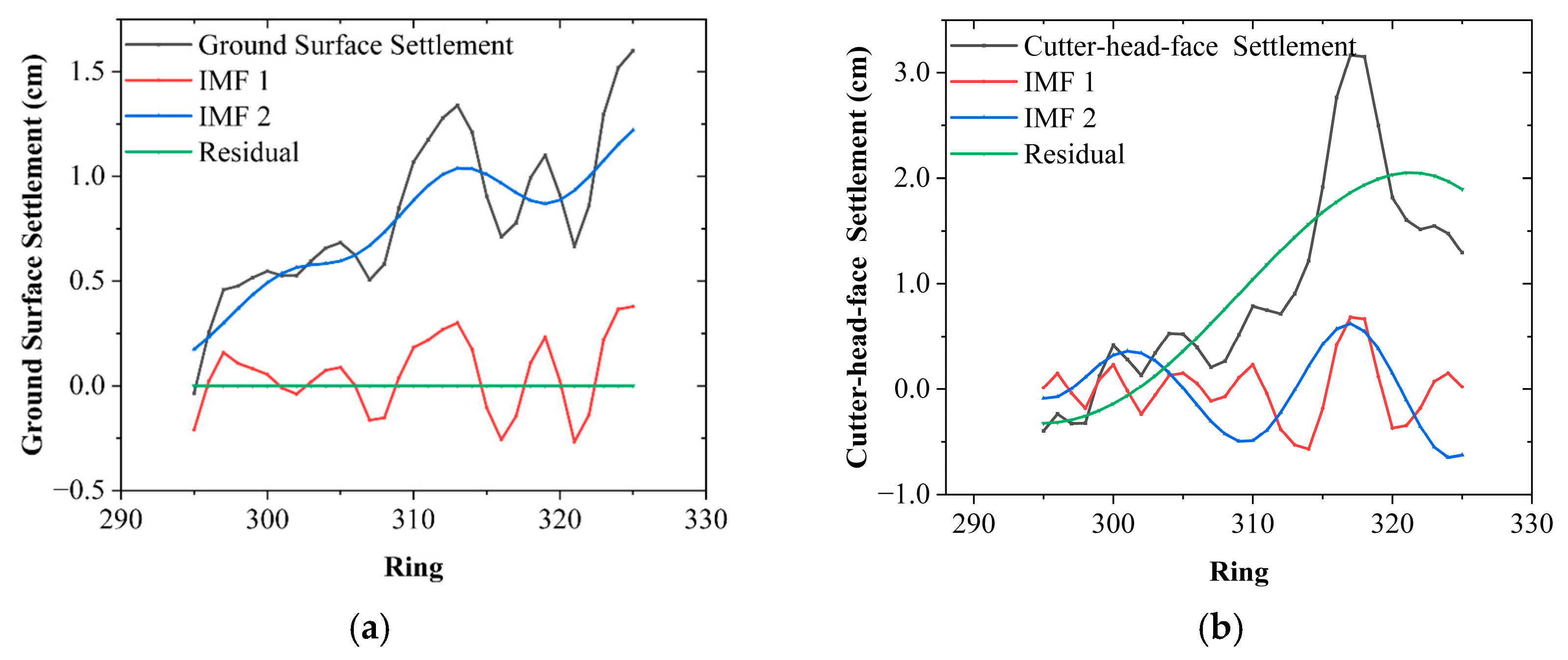
Figure 4a,b illustrates the EMD results of the original settlement signals. By decomposing nonlinear and non-stationary signals into several IMFs and one residual component, the EMD technique effectively reveals the multi-scale dynamic characteristics embedded in the settlement sequences.

In Figure 4a, the decomposition results of the raw surface settlement signal between ring number 300 and 320 are presented. The black curve represents the original settlement signal. Among the decomposed components, IMF 1 and IMF 2 capture the high-frequency and medium-frequency oscillations, respectively, reflecting short-term fluctuations caused by excavation disturbances. The residual term (green curve) describes the long-term trend of the settlement process. Notably, IMF_1 exhibits distinct periodic fluctuations, while IMF 2 shows a relatively smooth upward trend, suggesting a combination of cyclical disturbance and an overall downward movement in this segment.

Figure 4b shows the EMD results for the settlement data in front of the cutter-head. Compared to the surface data, IMF 1 and IMF 2 in this case are more dynamic, indicating that the ground surface disturbances during cutter-head advancement are more pronounced, resulting in higher frequency and larger amplitude responses. The residual term displays a rising trend that gradually stabilizes, revealing a dynamic process characterized by an intense short-term disturbance followed by long-term stabilization.

In summary, EMD effectively captures the multi-scale temporal features of the settlement signals and provides a theoretical and data-driven foundation for the construction of lag-based IMF features and the input variables of subsequent predictive models.

3.1.3. Lag Feature Engineering

When dealing with time-dependent settlement sequences, the current settlement behavior at a given ring is often significantly influenced by the settlement states of preceding rings. To more comprehensively model the temporal dependencies in settlement evolution, this study introduces a lag feature engineering strategy during the initial phase of data processing. This approach involves incorporating the historical values of the target variable as additional input features for the prediction model [32,33].

Specifically, based on the smoothed surface settlement sequence ${\tilde{y}}_t$ and using a set of lag features, a time window of length k (where k = 3) is constructed. In this study, the lag window was set to k = 3, consistent with engineering practice in shield tunneling, where the settlement response of a given ring is most strongly influenced by the preceding 3–4 rings and then rapidly attenuates. This choice balances capturing the dominant temporal memory while minimizing noise from rings farther back in the sequence, as follows:

$$\left\{\begin{array}{c}{\mathrm{Lag}}_1={\mathrm{y}}_{\mathrm{t}-1}\\ {\mathrm{Lag}}_2={\mathrm{y}}_{\mathrm{t}-2}\\ {\mathrm{Lag}}_3={\mathrm{y}}_{\mathrm{t}-3}\end{array}\right.$$

(3)

These variables represent the settlement information of the previous 1, 2, and 3 rings, respectively, and are incorporated as input features for the current ring $\mathrm{t}$ in the modeling process. The inclusion of lag features not only enables the model to capture the temporal patterns of settlement behavior in preceding segments, but also effectively mitigates the volatility and uncertainty associated with single-point predictions.

3.1.4. Feature Dimensional Reduction (PCA)

After the fusion of multi-source features, the input dimensionality of the model increases significantly. These features include shield tunneling parameters (e.g., thrust, torque, and advance rate), geotechnical parameters (e.g., density, compression modulus, and internal friction angle), EMD components, and constructed lag features. Although these high-dimensional features contain rich information, they also introduce issues such as dimensional redundancy, strong inter-feature correlation, and increased computational burden for the model.

To address these challenges, this study applies principal component analysis (PCA) to perform dimensional reduction on the high-dimensional feature set [34,35]. PCA is a classical linear dimensionality reduction technique that transforms the original feature space into a set of new variables known as principal components. These components are uncorrelated with each other and are ranked according to their ability to explain the variance in the original data [36].

During the dimensional reduction process, all numerical features are first standardized so that their mean is zero and standard deviation is one. This normalization ensures that features on different scales do not disproportionately affect the results. Then, a covariance matrix is computed from the standardized features, followed by eigenvalue decomposition. A subset of the principal components that collectively explains 95% of the total variance is selected as the new feature input. Let the original data matrix be denoted as follows:

$$\mathrm{X}\left[{\mathrm{x}}_1,{\mathrm{x}}_2,\dots ,{\mathrm{x}}_{\mathrm{p}}\right]\in {\mathrm{R}}^{n\times p}$$

(4)

Here, $n$ denotes the number of samples, and $p$ represents the number of original feature dimensions. First, the matrix $\mathrm{X}$ is centralized and standardized. Then, the covariance matrix $C$ is computed as follows:

$$\mathrm{C}={\displaystyle \frac{1}{\mathrm{n}-1}}{\mathrm{X}}^{\mathrm{T}}\mathrm{X}$$

(5)

Through eigenvalue decomposition (or singular value decomposition), the eigenvectors and eigenvalues of the covariance matrix are obtained. The eigenvector matrix $\mathrm{W}$ is then used to construct the principal component transformation. The resulting low-dimensional principal component matrix $\mathrm{Z}$ can be expressed as follows:

$$\mathrm{Z}=\mathrm{X}·{\mathrm{W}}_{\mathrm{k}}$$

(6)

where $\mathrm{X}$ is the standardized input matrix, and ${\mathrm{W}}_{\mathrm{k}}\in {\mathrm{R}}^{\mathrm{p}\times \mathrm{K}}$ is the matrix composed of the top $\mathrm{k}$ eigenvectors corresponding to the largest eigenvalues, such that the cumulative explained variance exceeds a predefined threshold (e.g., 95%). These principal components are then used as compact and informative inputs for the subsequent predictive modeling.

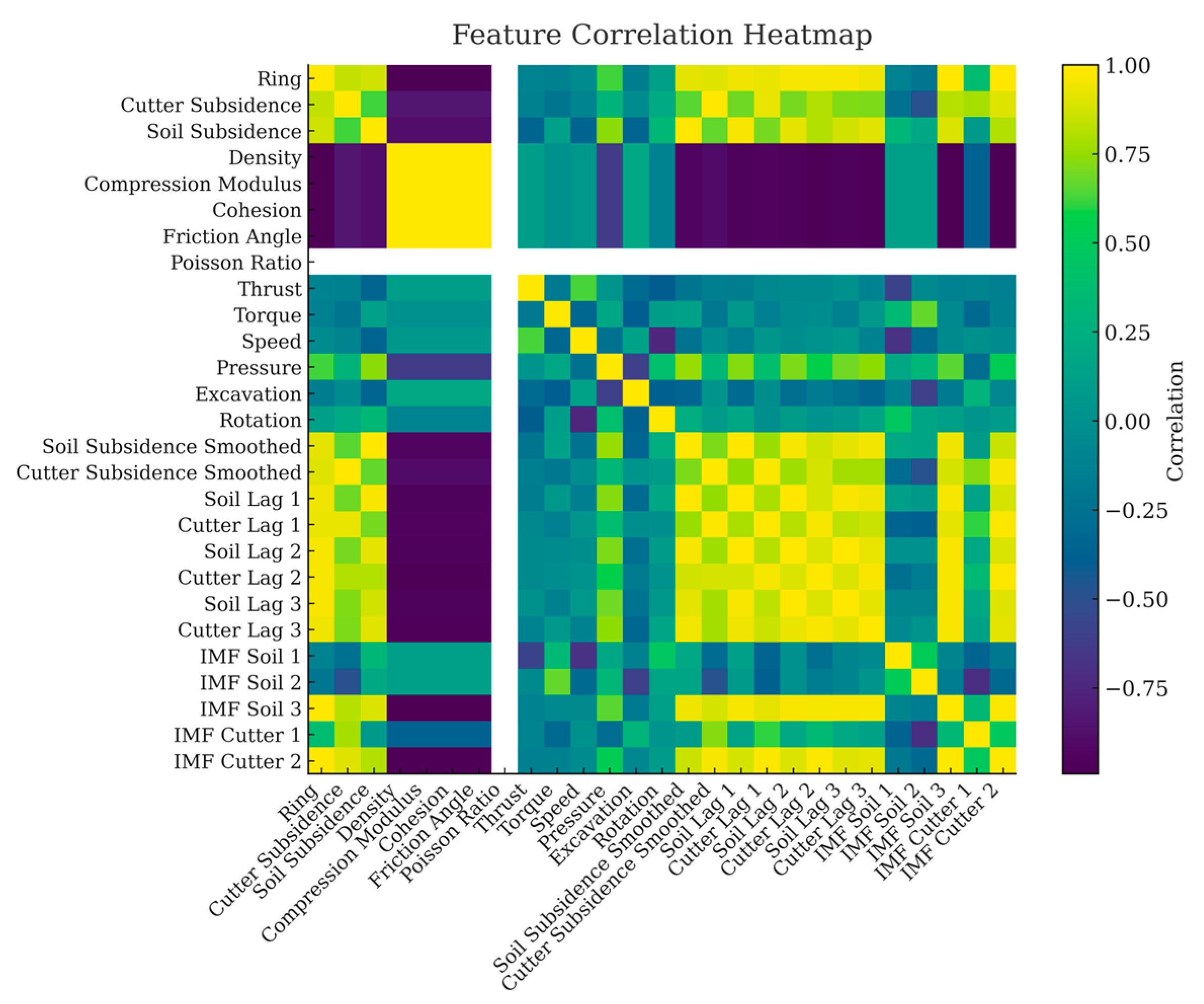
Figure 5 presents a correlation heat map of the model input variables, where the Pearson correlation coefficient is used to quantify the linear relationships between variable pairs. The color intensity reflects the magnitude and direction of the correlation: red indicates strong positive correlation (close to +1.0), blue indicates strong negative correlation (close to −1.0), and grayness represents moderate or weak correlation levels.

Among the input variables, the shield tunneling parameters—such as thrust, torque, and rotation speed—exhibit moderate positive correlations with one another. In contrast, geological properties such as density, cohesion, and compression modulus show significant negative correlations with the settlement measurements. Moreover, a clear banded structure is observed between the IMF components derived from EMD and the lag features (e.g., soil lag 1 to cutter lag 3), indicating a hierarchical and temporally dependent feature relationship. High correlations among lagged settlement features suggest redundancy, justifying PCA reduction.

Meanwhile, the correlations between soil settlement, cutter settlement, and ring number are relatively weak, suggesting that surface settlement is more influenced by the interaction between soil conditions and shield operational parameters rather than being controlled solely by the ring index. This insight provides a theoretical basis for feature selection in the subsequent construction of the graph neural network model, and highlights the importance of incorporating temporal windows and localized spatial awareness mechanisms in model design.

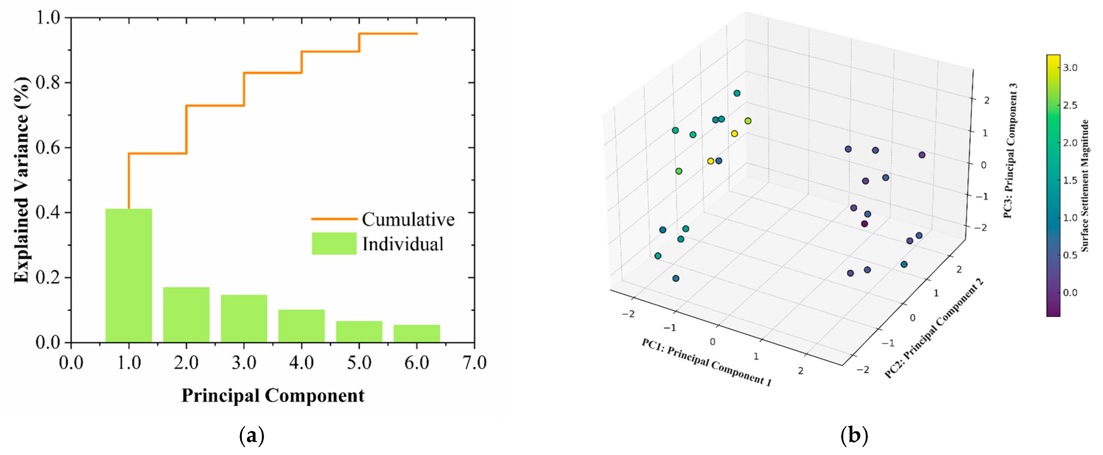
Based on the standardized construction parameters, soil and rock properties, and EMD-derived components, PCA decomposition was conducted. The top three principal components were selected as input features to ensure a high information retention rate while significantly reducing dimensional redundancy, thereby improving model training efficiency and enhancing predictive robustness.

Figure 6a illustrates the distribution of individual explained variance and cumulative explained variance for each principal component under the operating conditions of this study. The results show that the first two components together explain approximately 60% of the total variance in the original feature set, while the first three components cumulatively explain over 75%. This indicates that a low-dimensionality representation can retain the majority of relevant information while greatly compressing input data space. These findings confirm the feasibility and effectiveness of PCA in this study and provide a solid foundation for feature simplification and generalization in subsequent modeling processes.

Figure 6b presents a three-dimensional visualization of the feature space constructed by the top three principal components, with color encoding based on the magnitude of surface settlement. A clear clustering pattern and gradient distribution can be observed: samples with higher settlement values are densely distributed within specific regions, while those with lower values appear more scattered. This well-defined spatial separation structure indicates that the principal components not only preserve critical structural features from the original data but also possess strong separability and discrimination power, making them effective in supporting accurate prediction and classification of settlement behavior.

Principal component analysis (PCA) was applied to reduce redundancy and improve robustness. Although retaining components explaining 95% of the variance would include more than six principal components, empirical validation indicated that predictive performance did not improve beyond the first three. The top three components, which together explained ~75% of the total variance, were therefore retained. This choice captures the majority of relevant information while avoiding the noise and redundancy introduced by additional components.

Through PCA-based dimensionality reduction, the overall feature dimension was compressed and the modeling burden was reduced. Moreover, the construction of a discriminative, label-informed feature space provided a reliable foundation for improving the robustness and generalization capability of the proposed GCN-SSPM model.

3.1.5. Handling Missing Values

After completing the Gaussian-weighted moving average, lag feature construction, and empirical mode decomposition (EMD), several missing values appeared in the dataset. This was mainly due to two reasons: first, the construction of lag features depends on the availability of data from preceding rings, causing the initial few samples to have missing entries in some lag variables; second, the EMD process introduces boundary effects at the ends of the sequence, which may also result in NaN values in the intrinsic mode functions (IMFs) [37,38].

To ensure the consistency and completeness of the input features during model training, we employed a row-wise deletion strategy to remove observations containing missing values. The missing entries arose only in a very limited portion of the dataset, primarily from lag feature construction and the boundary effects of EMD. This method effectively eliminated potential training errors caused by incomplete data while preserving stable and reliable model training. Since these cases accounted for only a small fraction of the data, the overall information loss was negligible. We further examined the sensitivity of the results and confirmed that excluding these rows did not materially affect model performance.

3.2. Adjacent-Ring Graph Convolutional Network (GCN)

A graph convolutional network (GCN) is a type of neural network designed to process graph-structured data. Its unique advantage lies in its ability to aggregate each node’s own features together with those of its neighbors in a single propagation step, followed by a nonlinear transformation [39]. Compared to one-dimensional convolutional neural networks (1D CNNs) and long short-term memory networks (LSTMs), GCNs can more intuitively capture the coupling mechanisms between adjacent rings on the same cross-section.

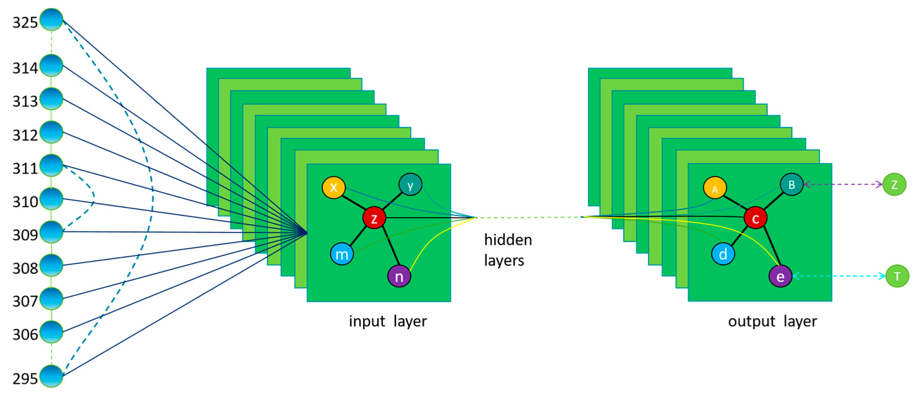
The model architecture consists of three main layers: an input layer, hidden layers, and an output layer. During the forward pass, each node updates its feature representation by aggregating information from its neighboring nodes. The network is trained to learn complex patterns and relational structures within the graph data. The structure is illustrated in Figure 7.

In this context, each shield ring is represented as a graph node v_i. Rings with adjacency relationships are connected via non-directional edges, resulting in a final chain-like graph structure.

$$G=\left(V,E\right),V=\left\{V_0,V_1,\dots ,V_{n-1}\right\},E=\left\{\left(i,i+1\right),\left(i+1,i\right)\left|0\le i\le N-1\right|\right\}$$

(7)

After adding self-loops, the adjacency matrix $\tilde{A}$ is constructed as follows:

$$\tilde{A}=A+I$$

(8)

where $A$ is the original adjacency matrix representing connections between neighboring rings, and $I$ is the identity matrix that introduces self-connections for each node. This formulation ensures that each node incorporates its own features during the message-passing process.

Each node is associated with a feature vector $Xi$, and the prediction target is the normalized surface settlement ${\tilde{y}}_i$. After feature construction and initial phase of processing, the data are encapsulated into a graph structure and fed into the GCN model for training and inference.

The GCN-SSPM model adopts a three-layer graph convolutional architecture, which aggregates information from each node and its six neighboring nodes—three preceding and three following ring nodes. This aggregation range corresponds to a physical influence radius of approximately ±3 rings. Such a setting is consistent with engineering practice and field observations: disturbances induced by shield lining responses tend to decay rapidly within several rings behind the cutter-head, and engineering reports indicate that TBM-induced effects generally dissipate after about ten rings. Thus, focusing on ±3 rings allow the model to capture the most significant local interactions while minimizing noise and over-smoothing, aligning with the widely observed empirical “3–4 ring influence width” in shield tunneling.

In addition, the progressive dimensionality reduction strategy enables the network to automatically perform feature selection during neighborhood aggregation, thereby reducing the risk of over-fitting. Specifically, the feature dimension is reduced from 64 to 32 and then to 16 across the three GCN layers. This hierarchical compression filters redundant or irrelevant information while preserving meaningful patterns.

To capture nonlinear interactions, a ReLU activation function is applied after each graph convolution layer. The use of ReLU enhances the network’s capacity to learn complex, nonlinear relationships, thereby improving its expressive power and adaptability.

The key architectural and parameter configurations of the model are summarized in

Table 2. GCN-SSPM architecture parameters.

Stage	Operation	Output Size
Input	Feature tensor after preprocessing, EMD, PCA, lags, etc.	31 × 30 ($N,F$)
Graph Construction	Bidirectional edge list based on adjacent ring connections	2 × 60 (2,2 × ($N$ − 1))
GCN Layer 1	GCN Conv (input dim → 64), ReLU	31 × 64 ($N$, 64)
GCN Layer 2	GCN Conv (64 → 32), ReLU	31 × 32 ($N$, 32)
GCN Layer 3	GCN Conv (32 → 16), ReLU	31 × 16 ($N$, 16)
Fully Connected	Linear (16 → 1)	31 × 1 ($N$, 1)
Output	Predicted surface settlement per ring	31 ($N$)

Note: $N$ denotes the number of shield rings (e.g., 31), and $F$ is the number of input features per ring after preprocessing (e.g., 30). The graph is constructed as a bidirectional chain structure, where each node represents a ring and is connected to its adjacent rings (e.g., ring $i$↔ ring $i+1$), yielding 2 × (N − 1) edges.

.

This study evaluates the predictive performance of the proposed GCN-SSPM model on a real-world shield tunneling surface settlement dataset. All models were trained from scratch for 300 epochs. The GCN-SSPM was trained using a full-graph approach, and the Adam W optimizer was applied consistently across models, with hyperparameters set to β1 = 0.9 and β2 = 0.999. An L2 weight decay of 1 × 10⁻⁴ was applied to all trainable parameters to improve generalization. To prevent over-fitting under small-sample conditions, the LSTM-based model incorporated dropout (with a dropout rate ε = 0.2) and an attention mechanism. In contrast, GCN-SSPM inherently enforced high-order spatial topological constraints through its three-layer convolutional architecture. During training, gradient clipping (with a maximum norm of 1.0) was used to prevent gradient explosion, and an exponential moving average (EMA) of model weights (decay factor = 0.999) was introduced to enhance stability and consistency during inference.

The dataset was split into 80% training and 20% validation, with all hyperparameters tuned based on validation performance. The validation set consisted of settlement data from the last 20% of shield ring numbers to ensure a realistic scenario and to prevent future data leakage. No data augmentation or additional training tricks were used, ensuring the experiment’s rigorous, reproducible, and focused nature. Due to the time-series nature of data and its limited length, we opted against k-fold cross-validation. We also avoided random shuffling to prevent any risk of temporal leakage between training and testing sets. All preprocessing operators (Gaussian smoothing parameters, EMD IMF selection, scaling, and PCA fitting) were estimated on the 80% training portion only and then applied unchanged to the last-20% subset. RMSE, MAE, and R² were calculated on this chronological hold-out (the last 20% of the “time-reserved test set”). All baselines (LSTM+GRU+Attention and XGBoost) follow the same split and preprocessing. As a limitation, we use a single chronological hold-out rather than multi-fold CV or an external test set.

3.3. Multi-Model Comparison and Ensemble Fitting

To further improve prediction accuracy and generalization, this study introduces a dynamic weighted ensemble (DWE) method based on the outputs of multiple trained models. This approach dynamically adjusts the contribution of each base model to the final prediction by inversely weighting their local prediction errors within a sliding window around each ring segment [40,41].

Assuming there are M predictive models and the smoothed error of the m-th model in the time window centered at step t is given (${\mathit{MSE}}_{\mathit{m},\mathit{t}}$), then the m-th model weight ${\omega }_{\mathit{m},\mathit{t}}$ of the t-th sample is calculated as follows;

$${\omega }_{m,t}={\displaystyle \frac{1/\left({MSE}_{m,t}+\epsilon \right)}{{\sum }_{j=1}^{M}1/\left({MSE}_{j,t}+\epsilon \right)}}$$

(9)

In the implementation of Equation (9), the sliding window was designed as a causal window. When making predictions at a given ring, the weighting scheme only refers to the prediction errors from the most recent w rings before the current one. No future rings are included in the calculation. This design ensures that the weights depend solely on past information and prevents any potential information leakage during training and testing. $\mathsf{ϵ}={10}^{-6}$ is a small constant added to prevent division by zero. These weights are updated dynamically within a fixed window size, based on each model’s historical performance, thereby enhancing adaptability and robustness in the ensemble prediction. Then, the commonly used LSTM+GRU+Attention and XGBoost models are fitted and compared [42,43,44].

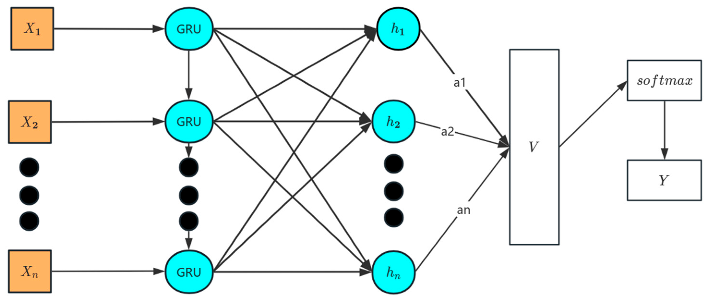
For the models, we adopted systematic hyperparameter tuning procedures to ensure a fair comparison with GCN-SSPM. For the LSTM+GRU+Attention model, we performed grid search with early stopping on the validation set. The search space included hidden units {32, 64, 128}, dropout rates {0.2, 0.3, 0.5}, and learning rates {1 × 10⁻⁴, 5 × 10⁻⁴, 1 × 10⁻³}, and the optimal configuration was determined based on the lowest validation loss, and the Flowchart of the LSTM+GRU+Attention modeling algorithm is shown in Figure 8. For XGBoost, we tuned the number of estimators (100–500), maximum tree depth (3–8), learning rate (0.01–0.3), subsample ratio (0.6–1.0), and colsample_bytree (0.6–1.0). The best parameters were selected using validation RMSE as the criterion. Importantly, both baseline models were trained under the same chronological data split and feature preprocessing pipeline (Gaussian smoothing, EMD, lag features, and PCA) as GCN-SSPM, ensuring fairness and comparability across models.

All neural network models were trained from scratch for 300 epochs using the Mean Squared Error (MSE) loss function. Optimization was performed with the AdamW optimizer (β1 = 0.9, β2 = 0.999) and an L2 weight decay of 1 × 10⁻⁴. The initial learning rate was set to 1 × 10⁻³ for the LSTM+GRU+Attention model and 5 × 10⁻³ for the GCN-SSPM, with the rate reduced on plateau. A batch size of 8 was used for the sequence models, and early stopping was triggered if validation loss did not improve for 50 consecutive epochs.

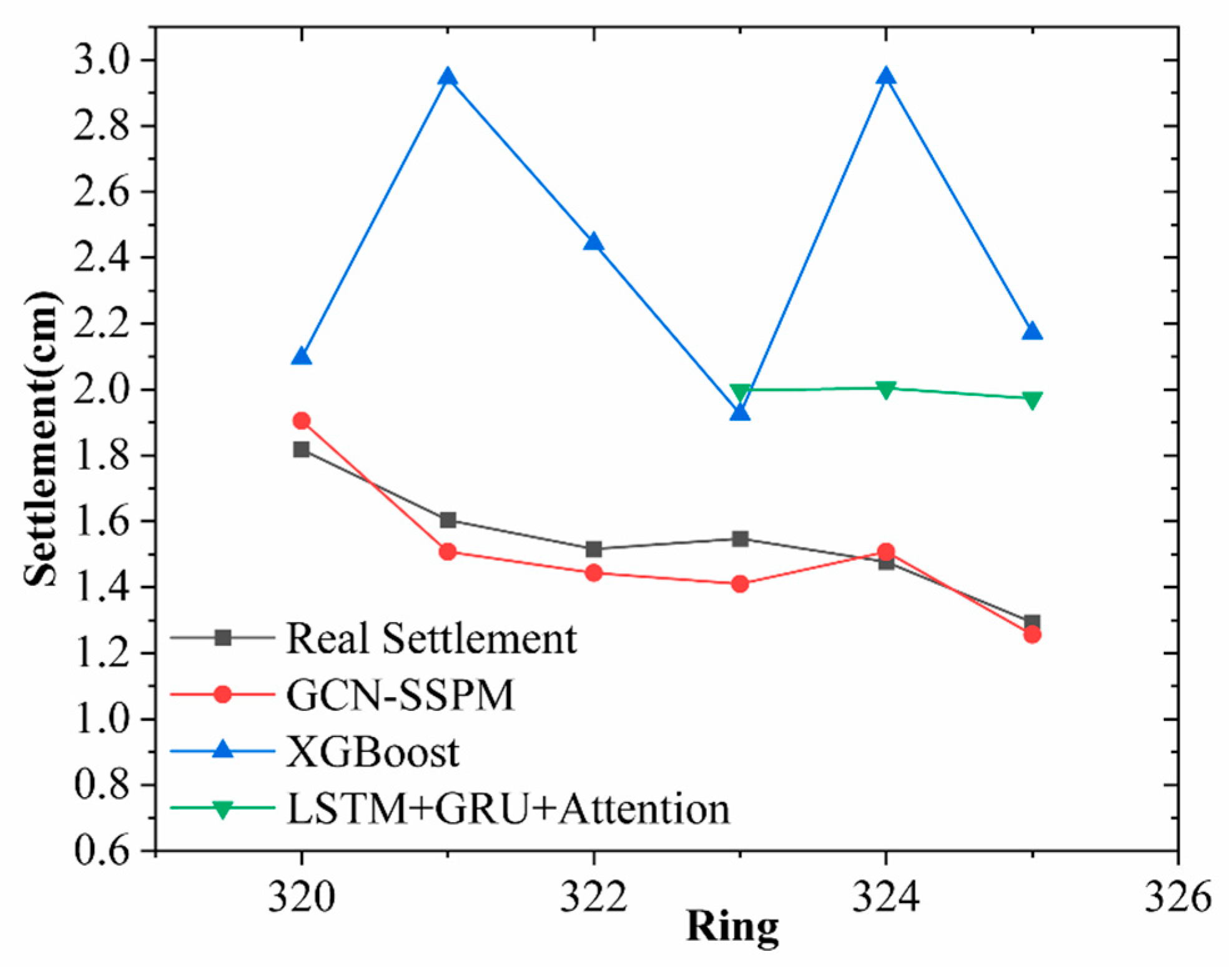
Figure 9 compares the predicted settlement results from the GCN-SSPM, LSTM+GRU+Attention, and XGBoost models against the actual measurements. The black solid line represents the observed surface settlement; the red, green, and blue lines represent predictions from GCN-SSPM, LSTM+GRU+Attention, and XGBoost, respectively.

Figure 9 shows that GCN-SSPM closely tracks the measured settlement trends across multiple ring numbers (e.g., rings 321 and 324), accurately capturing the magnitude and shape of local fluctuations. In contrast, XGBoost tends to overestimate in several regions, indicating weaker strength when modeling data with a significant time and space relationship. The LSTM+GRU+Attention model captures the overall trend to some extent, but its prediction curve appears overly smoothed and fails to reflect local disturbance effects effectively. Under the small-sample, high-noise conditions, the sequence-only model (LSTM+GRU+Attention) and tree-based model (XGBoost) yield negative R² values, indicating poor generalization. In contrast, GCN-SSPM achieves millimeter-level precision with RMSE = 0.09 cm, MAE = 0.08 cm, and R² ≈ 0.71 and the predictive performance of the three models is presented in

Table 3. Comparison of predictive performance among different models.

Model	RMSE (mm)	MAE (mm)	R2	Notes
GCN-SSPM	0.085	0.077	0.71	Chronological hold-out (last 20% rings data)
LSTM+GRU+Attention	0.984	0.879	<0
XGBoost	0.365	0.345	<0

; the rolling-origin cross-validation setup is shown in

Table 4. Rolling-origin cross-validation.

Type	RMSE	MAE	R2
GCN-SSPM	0.085 ± 0.02	0.077 ± 0.02	0.71 ± 0.08
LSTM+GRU+Attention	0.984 ± 0.3	0.879 ± 0.25	<0 (unstable)
XGBoost	0.365 ± 0.10	0.345 ± 0.09	<0

. Based on these results, set k=3 as the optimal choice. To improve statistical reliability given the small sample size, rolling-origin evaluation was performed. The dataset was split into consecutive test blocks, each predicted using all prior rings for training. Table 4 reports the mean ± standard deviation of RMSE, MAE, and R² across these blocks. GCN-SSPM consistently achieved a low error and stable R², whereas baseline models showed large variability and poor generalization.

Overall, the GCN-SSPM outperforms the baseline models in both accuracy and generalization, offering more reliable technical support for risk assessment and control in shield tunneling operations.

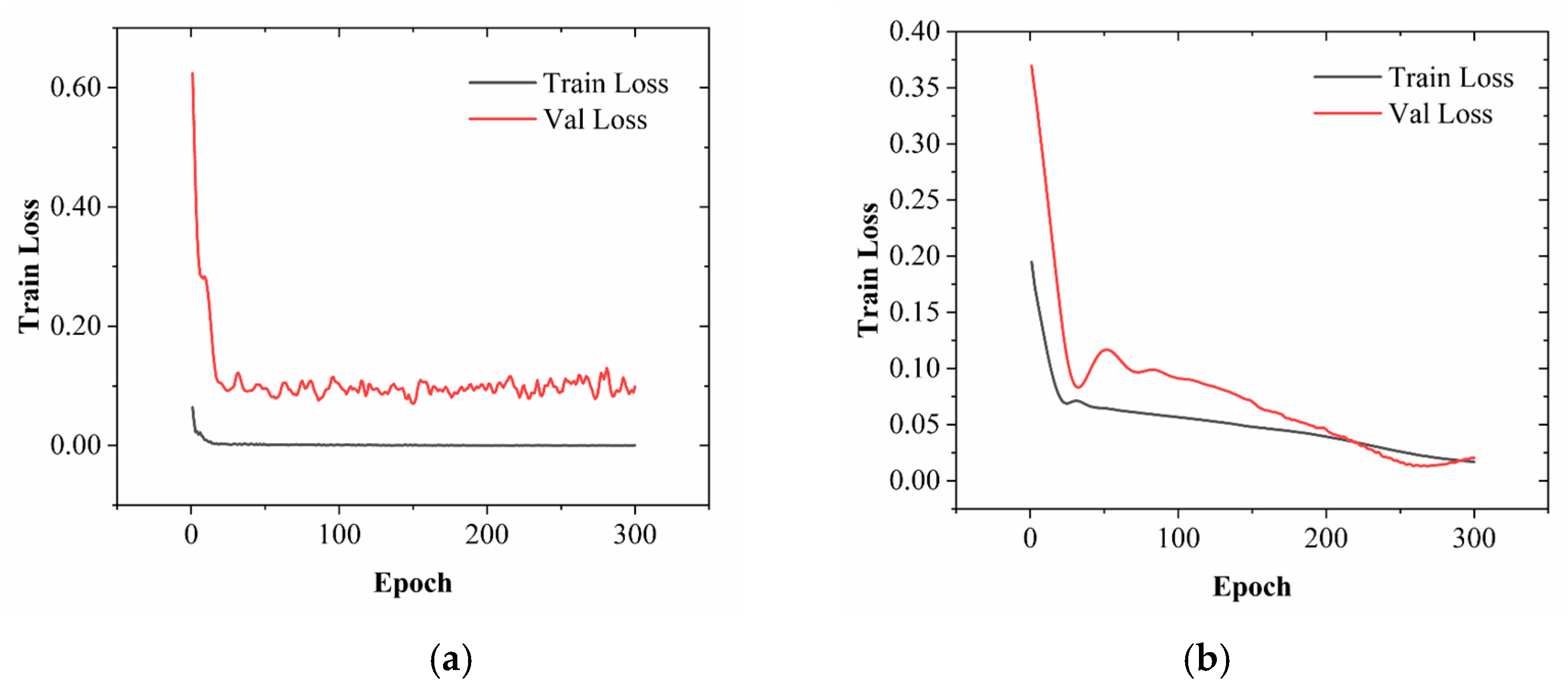
Figure 10 presents the training loss curves for the LSTM+GRU+Attention model and the GCN-SSPM model, used to evaluate model fitting performance and generalization capability in shield tunneling settlement prediction.

As illustrated in Figure 10a, the LSTM+GRU+Attention model demonstrates a rapid decline in training loss within the first 100 epochs, decreasing from an initial value of approximately 0.1 to below 0.01, and ultimately converging to the order of 10⁻⁴. This trend indicates that the model exhibits strong learning capacity on the training dataset, effectively capturing the temporal evolution patterns of shield tunneling-induced settlement. However, the validation loss remains persistently high, fluctuating between 0.08 and 0.12. Despite a minor decrease during the early training phase, no sustained improvement is observed thereafter, and fluctuations persist through later epochs. This behavior suggests that, although the model performs well in time series modeling, it lacks the capacity to exploit spatial structural information, particularly the inter-ring dependencies inherent in shield tunneling processes. Consequently, the model’s generalization capability on unseen data is significantly restricted under complex and non-stationary geological conditions.

By contrast, Figure 10b presents the loss evolution curves for the GCN-SSPM model under identical training conditions, which display superior convergence characteristics and stability. The training loss decreases sharply from 0.195 to 0.057 within the first 50 epochs and continues to decline steadily to below 0.002, reflecting fast convergence and robust training performance. More importantly, the validation loss experiences a substantial reduction from 0.370 to approximately 0.028 during the first 100 epochs and reaches a minimum at around epoch 150. Although a slight rebound is observed beyond epoch 200, where it fluctuates between 0.04 and 0.08, the validation loss was slightly lower than the training loss during certain intervals. This behavior arises from the use of exponential moving average (EMA) smoothing of model weights and regularization strategies, which stabilize validation performance and can occasionally yield lower validation loss compared to the raw training curve. This indicates that GCN-SSPM not only avoids over-fitting but also maintains strong generalization capability. The observed performance can be attributed to the model’s integration of graph convolutional layers, which enable it to capture local spatial correlations and structural patterns across adjacent rings. These characteristics enhance its robustness to data noise and its adaptability to multi-source disturbances, making GCN-SSPM particularly well-suited for small-sample, high-noise settlement prediction tasks in shield tunneling projects.

In summary, by incorporating an adjacency-based graph structure, GCN-SSPM effectively models spatial topological dependencies and demonstrates superior convergence and generalization performance compared to traditional time-series-based deep learning models, particularly in scenarios involving sudden settlement shifts and nonlinear evolution patterns.

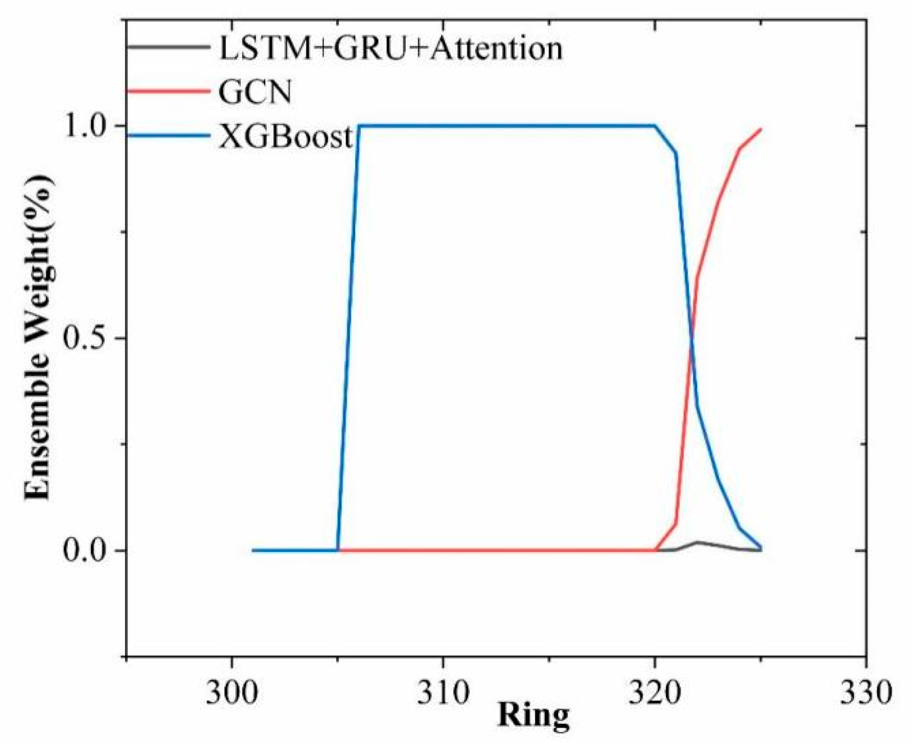
Figure 11 illustrates the evolution of ensemble weights assigned to each model across the full tunneling sequence, reflecting the changing contributions of individual models at different shield rings. Ring 320 serves as the boundary between the training and testing sets, with the region to the right representing the model’s predictive performance on unseen data.

During the training phase (ring < 320), the XGBoost model dominates most intervals with weights approaching 1, suggesting the lowest fitting error on known samples. This is attributed to XGBoost’s tree-based structure, which excels in capturing static features and nonlinear patterns under sufficient training data. In contrast, two fusion models GCN-SSPM and LSTM+GRU+Attention both obtain near-zero weights during training, indicating their limited advantage in fitting stable patterns.

However, after entering the testing phase (ring ≥ 320), the weight distribution shifts significantly: GCN-SSPM quickly becomes the dominant contributor, while XGBoost’s weight drops sharply. This transition is driven by increased geological disturbance and complex settlement patterns in the later tunneling stages, where static models struggle to maintain performance. GCN-SSPM’s graph-based structure enables it to capture ring-to-ring spatial interactions and disturbance propagation, thereby demonstrating stronger adaptability and robustness under evolving conditions.

LSTM+GRU+Attention gains a slight increase in weight in the testing set but contributes relatively little overall. This suggests that while it offers partial assistance via temporal feature extraction in certain local windows, it lacks the capacity to fully model spatial structural evolution.

In conclusion, the adaptive weight distribution confirms the ensemble strategy’s ability to dynamically identify and leverage the locally optimal model. It further validates that GCN-SSPM’s strength lies in its structure-aware capability, rather than mere data-fitting performance.

Figure 12 presents the final ensemble prediction compared with the actual settlement values. The ensemble curve closely aligns with the measured trend and accurately responds to sudden settlement changes, such as those observed at rings 318 and 320. The shaded blue region represents the 95% confidence interval, which was constructed from the weighted variance of the dynamic ensemble predictions across the three base models. Calibration analysis revealed that the empirical coverage rate of the interval was close to the nominal 95% level, and the continuous ranked probability score (CRPS) indicated good probabilistic reliability. These results confirm that the ensemble model not only captures the settlement trend but also provides well-calibrated uncertainty quantification, enhancing its reliability and applicability in practical engineering scenarios.

4. Results and Discussion

To evaluate the effectiveness of the GCN-SSPM model in predicting shield tunneling-induced surface settlement, this study conducted experiments using real-world data from a typical section of the Wuhan Metro. The model was trained using actual settlement records and shield operation parameters, and its performance was compared with that of LSTM+GRU+Attention and XGBoost models across multiple evaluation metrics, including prediction accuracy, responsiveness to abrupt changes, training convergence behavior, and robustness.

In terms of overall trend fitting, GCN-SSPM outperformed the baseline models, especially in regions exhibiting abrupt settlement changes. It accurately captured the location and amplitude of settlement inflection points. By contrast, the XGBoost model tended to over-smooth or overestimate predictions across many segments, revealing limitations in modeling nonlinear spatially dependent patterns. The LSTM+GRU+Attention model, while effective in capturing temporal trends, lacked structural awareness of shield ring interactions, resulting in unstable predictions in geologically complex zones.

From the perspective of training stability and convergence, GCN-SSPM demonstrated faster convergence and lower overall loss compared to other models. Its validation loss showed a continuous decline and remained lower than the training loss throughout, indicating strong generalization capability. In contrast, the sequence-based LSTM+GRU+Attention model exhibited greater fluctuations between training and validation loss, suggesting a tendency toward excessive fitting.

The dynamic weighted ensemble strategy further improved adaptability under varying ground surface conditions. By assigning model weights based on local error within a sliding window, the ensemble could selectively emphasize GCN-SSPM in zones with high disturbance, while integrating predictions from LSTM and XGBoost in more stable regions. This strategy enhanced both global robustness and local accuracy, offering reliable support for risk warning and construction control during tunneling.

Thanks to its structure-aware modeling, fast convergence, and understandable nature, the GCN-SSPM model demonstrates strong potential for accurate settlement prediction under small-sample and spatially coupled conditions. It shows good applicability for real-world shield tunneling projects and contributes to the advancement of intelligent construction practices.

5. Conclusions

This study addresses the challenges of small-sample, high-noise, and strongly non-stationary settlement monitoring data commonly encountered in shield tunneling projects. An adjacent-ring GCN architecture leverages the physical ring-to-ring disturbance propagation, rather than treating settlement purely as a temporal sequence. A small-sample prediction model based on adjacent-ring graph convolutional networks (GCN-SSPM) is proposed, achieving prediction accuracy ≥90%, with its performance validated through comparative experiments against multiple baseline models. The findings can be summarized as follows:

(1)

During the preparation of data and feature engineering, Gaussian-weighted smoothing effectively reduces high-frequency noise. Empirical mode decomposition (EMD) extracts multi-scale intrinsic mode functions (IMFs), while lag features and principal component analysis (PCA) construct a feature matrix capturing temporal memory and multi-scale responses, providing robust input support under small-sample conditions.

(2)

For model architecture, the shield ring sequence is structured as a graph, and a three-layer GCN aggregates spatial topological information from neighboring rings (within a three-ring radius). Compared to LSTM+GRU+Attention and XGBoost, GCN-SSPM demonstrates superior convergence speed, prediction accuracy, and generalization capability.

(3)

In baseline model comparison: LSTM+GRU+Attention effectively models sequential trends but lacks spatial awareness; XGBoost performs well in stable zones yet fails in abrupt settlement regions due to limited spatial dependency modeling. GCN-SSPM’s graph structure enhances the perception of spatial disturbances, achieving higher accuracy and stability in critical zones.

(4)

A dynamic weighted ensemble strategy employs an adaptive mechanism to adjust the model contributions based on local prediction errors within a sliding window. This approach leverages the complementary strengths of sub-models, improving overall consistency and adaptability, especially in regions with sudden settlement changes.

GCN-SSPM establishes a systematic framework for spatial disturbance modeling, feature engineering, and intelligent ensemble learning in shield tunneling. It advances settlement prediction under small-sample constraints and offers an effective solution for risk modeling and decision making in complex urban geological environments, significantly contributing to intelligent construction theory and practice.

Nevertheless, this study has several limitations. The monitoring dataset does not include groundwater level or pore-water pressure information, although groundwater is known to play a critical role in tunneling-induced settlement, especially in soft ground conditions. The validation was conducted on a single right-line section influenced by a staged excavation of the left line, and the sample size remains relatively small. As a result, the reported accuracy should be regarded as case-specific and best applied to projects under geological and operational conditions similar to those of the Wuhan Metro case. In addition, the preprocessing pipeline (e.g., Gaussian smoothing, IMF selection in EMD, and PCA thresholds) may introduce sensitivity to parameter settings, and the present analysis focused on post-hoc uncertainty estimation without providing prior uncertainty quantification. Future work may therefore extend the framework by incorporating groundwater monitoring or coupled hydro-mechanical simulations, adopting multi-line graphs with cross-sectional edges to capture 3D interactions, developing causal ensemble strategies for clearer model integration, designing physics-guided loss terms to embed engineering priors, validating across different geological settings, and evaluating cost-effectiveness for field deployment. These steps will further strengthen the robustness, explainability, and practical relevance of GCN-SSPM. It is also worth noting that the PCA components and the dynamic ensemble weight evolution are consistent with geotechnical mechanisms: the first two principal components reflect load–layer interactions and multi-scale disturbances, while the ensemble weight shift coincides with staged excavation effects. These qualitative correspondences suggest that the learned representations align with established soil–structure interaction patterns.