Article

Hyper-Localized Pollution Mapping Using Low-Cost Wearable Monitors and Citizen Science in Hong Kong

by
Xiujie Li
1,
Cheuk Ming Mak
1,*,
Yuwei Dai
2,
Kuen Wai Ma
1 and
Hai Ming Wong
3
1
Department of Building Environment and Energy Engineering, The Hong Kong Polytechnic University, Hong Kong
2
School of Environment and Architecture, University of Shanghai for Science and Technology, 516 Jungong Road, Shanghai 200093, China
3
Faculty of Dentistry, The University of Hong Kong, Hong Kong
*
Author to whom correspondence should be addressed.
Buildings 2025, 15(17), 3131; https://doi.org/10.3390/buildings15173131
Submission received: 28 July 2025 / Revised: 29 August 2025 / Accepted: 31 August 2025 / Published: 1 September 2025
(This article belongs to the Section Building Energy, Physics, Environment, and Systems)

Abstract

Low-cost sensors have demonstrated their advances in acquiring hyper-localized data compared to traditional, high-maintenance air quality monitoring stations. The study aims to leverage the mobility of participants equipped with low-cost wearable monitors (LWMs) by comparing their exposure to particulate matter (PM) across indoor-home, outdoor-walking, and hybrid-commuting micro-environments. The LWMs would be calibrated first through field co-location and the multiple linear regression models. The coefficient of determination (R2) of PM1.0 and PM2.5 increased to over 0.85 after calibration, along with the reduced root mean square error of 2.25 and 3.46 μg/m3, respectively. The 26-day PM data collection with geographic locations could identify individual exposure patterns, local source contributions, and hotspot maps. Commuting constituted a small fraction of daily time (4–8%) but contributed a disproportionate impact, accounting for 11% of individual PM exposure. Indoor-home PM2.5 exposure varied significantly among the urban districts. Based on the PM2.5 hotspot map, the elevated concentration was mainly concentrated in dense residential areas and historical industrial areas, as well as interchanges of major roads and the highway system. LWMs acting as non-regulatory instruments can complement monitoring stations to provide missing short-term and hyper-localized air pollution data. Future studies should integrate long-term monitoring and citizen science across seasons and geographical regions to address pollutant spatiotemporal variability for building and city sustainability.

Graphical Abstract

1. Introduction

Particulate matter (PM) significantly affects human health, especially in the respiratory and cardiovascular systems [1,2]. Based on the recent report by the European Environmental Agency [3], over 95% of urban populations are exposed to highly delicate particulate matter, exceeding the annual average value (5 μg/m3) recommended by the World Health Organization (WHO) [4]. Personal exposure and health burden assessment is commonly evaluated from the particle mass concentration in different size fractions [5], like PM1.0, PM2.5, and PM10. The PM2.5 (fine particles) and PM1.0 (ultrafine particles) predominantly originate from combustion-related processes, including vehicular emissions and biomass burning [6,7]. The fine particles pose significant health risks as they can penetrate the lungs, veins, and circulatory system [8]. Therefore, accurately monitoring the concentration of fine particles in indoor and outdoor environments is critical for mitigating human exposure and safeguarding public health [9,10].
The currently widely used air quality monitoring stations mainly rely on the Federal Reference Method (FRM) and Federal Equivalent Method (FEM) techniques [11], which are capable of measuring changes in ambient PM concentration continuously and simultaneously. However, this monitoring instrument is quite expensive and large to move, which makes it less likely for the individual to monitor their living and working environments [12]. For example, Hong Kong is one of the most densely populated cities, with only eighteen fixed monitoring stations. Each station generally covers 100,000 to 600,000 residents to provide evidence for developing management and control policies. The recent development of technology in low-cost sensors can create revolutionary changes in the monitoring strategies [13]. The compact size, cost efficiency, low-energy consumption, and easy deployment characteristics have promoted its application for the automated air quality monitoring and IoT devices [14,15]. Integrating low-cost sensors and citizen science can encourage the general public to manage their local environments, detect primary pollution sources, and develop countermeasures. Examples include black carbon, PM, and total volatile organic compounds (TVOC) measurements performed by low-cost sensors mounted on bikes [16], tram-based mobile sensors in Zurich [17], taxi-based networks in Shanghai [18], etc. However, the deployment of low-cost sensors in regulatory measurement involves calibration and performance analysis, due to the sensitivity to meteorological variables [19,20]. Hofman et al. [21] indicated that the accuracy of low-cost sensors worsened by applying laboratory calibration, but was optimized further based on field calibration. Therefore, the deployment of low-cost sensors should be calibrated and co-located first with the reference instrument in representative environments. The calibrated hyper-localized pollution data can further provide evidence for implementing environmental policies at the community level, achieving urban sustainability.
Regulating indoor air quality (IAQ) presents unique complexities compared to outdoor environments [22], compounded by several interrelated challenges. A primary barrier is the lack of cost-effective monitors capable of deployment across diverse indoor spaces and human micro-environments. Traditional monitoring instruments such as FRM and FEM are pretty expensive and technically complex, rendering them ill-suited for hybrid monitoring across indoor and outdoor environments. Second, the vast majority of low-cost sensor applications are dedicated to the outdoor air monitoring networks. The potential can be further extended to short-term exposure events and occupational exposure monitoring [23,24]. A recent USA survey indicated that only a few low-cost and wearable air quality monitors are available on the market [12]. Scientifically sound investigations are yet to capture hyper-local pollution gradients influenced by traffic emissions, human activities, and indoor–outdoor transitions. Therefore, integrating LWMs and citizen science can offer a promising alternative for tracking short-term exposure events in different city environments.
Here, the case of Hong Kong for 26-day tracking was adopted with geographic locations, ambient environmental conditions, and PM concentrations. Participants will carry the LWMs daily to monitor air quality in their micro-environments and short-term exposure events. The interplay between human mobility, micro-environments, and personal exposure can be further elucidated by integrating global positioning system (GPS) data with continuous logging of particulate matter (PM1.0, PM2.5, PM10). This study aims to evaluate the performance of LWMs for monitoring PM concentrations in different micro-environments and to assess their reliability in capturing spatial and temporal variations in air quality across heterogeneous urban areas. The LWMs were first calibrated to enhance their accuracy through the field co-location with a reference instrument. The personal PM exposure characteristics were compared in different micro-environments: indoor-home, outdoor-walking, and hybrid-commuting. The PM concentration hotspot map over the sampling area was output by combining the environmental and geospatial information. This paper comprehensively evaluates LWMs for hyper-localized air quality monitoring and provides insights into integrating citizen participation to improve spatial coverage.

2. Materials and Methods

2.1. Wearable Strategies

The present study utilizes the Atmotube Pro as LWMs to measure ambient air quality continuously. The cost of an Atmotube Pro was USD 200, and a sensor costing less than USD 1000 can be regarded as a low-cost sensor [25]. The dimension of the LWM is around 8.6 cm × 5 cm × 2.2 cm, and the weight is only 104 g. As presented in Figure 1, the LWM was placed on the upper half of the human chest near the breathing zone region [26]. Table 1 illustrates the measurement and sensor characteristics. Based on the laser light-scattering principle, the sensor would calculate particle mass and number density within its measurement chamber. The PM1.0 and PM2.5 are measured directly, while the PM10 concentration is measured indirectly based on calculations and particle distribution profiles [27]. The ambient temperature, relative humidity (RH), and barometric pressure can be simultaneously captured. This monitor has been widely adopted in diverse scenarios, demonstrating moderate correlation and high precision in prior studies [28,29]. The integration with smartphones via Bluetooth can provide real-time GPS. Data acquisition supports offline storage and automated upload to cloud-based APIs for further analysis.
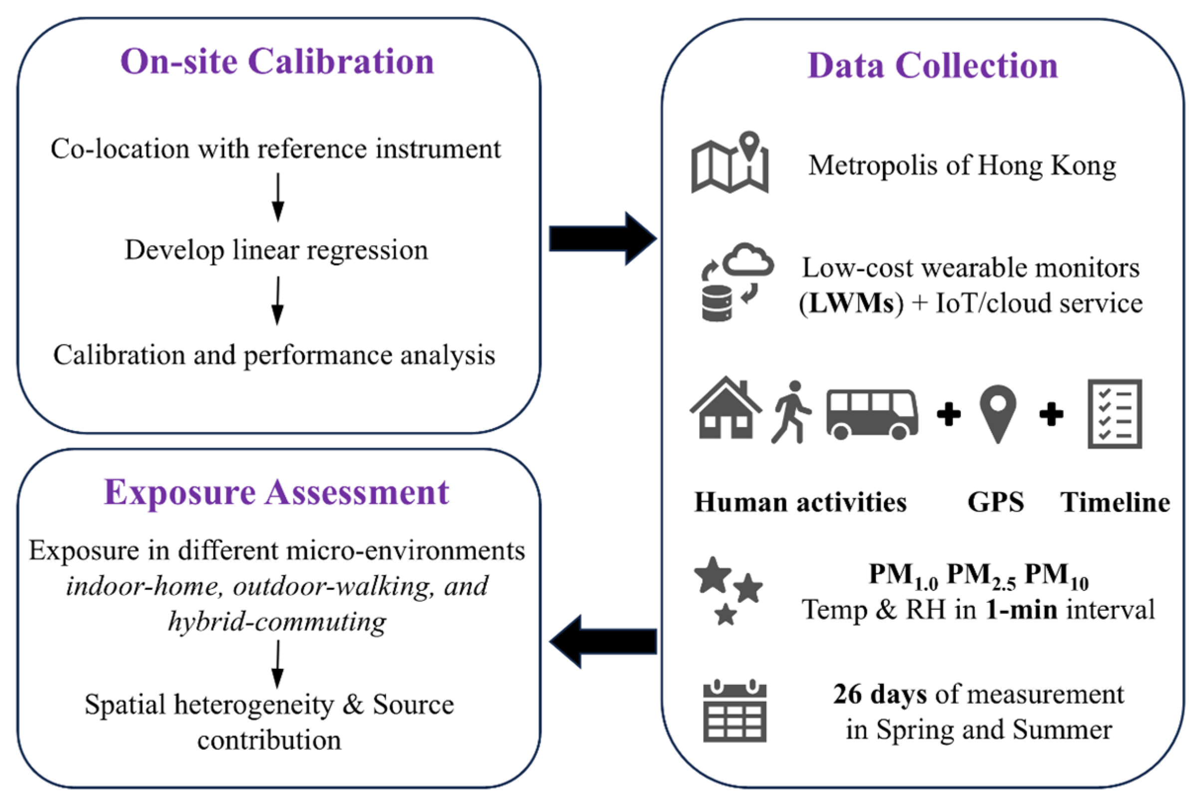
As shown in Figure 2, the research work was conducted in three steps: (a) onsite calibration; (b) mobile data collection; (c) exposure assessment. All of the LWMs need to be calibrated first before pollution data is collected. A gravimetrically pre-calibrated aerosol analyzer (Aerocet 532, MetOne Instruments, Inc., Grants Pass, OR, USA) was adopted as the reference for PM measurement. The Aerocet 532 underwent calibration in a laboratory setting using ideal polystyrene latex spheres, and the measurement accuracy was maintained within 10% of the laboratory sample. Then, the three LWMs would be co-located with the reference device in one residential home for four days. The RH fluctuated in the range of 50–70% during the field measurement and co-location. Each monitor was set at a 15 cm physical distance to minimize the disturbance of pumped airflow and ensure the homogeneous distribution of suspended particles. The sampling interval of one minute is determined by the sensor specifications and environmental dynamics, especially considering that the 1 min resolution can capture most exposure events [30].

2.2. Data Collection and Measurement

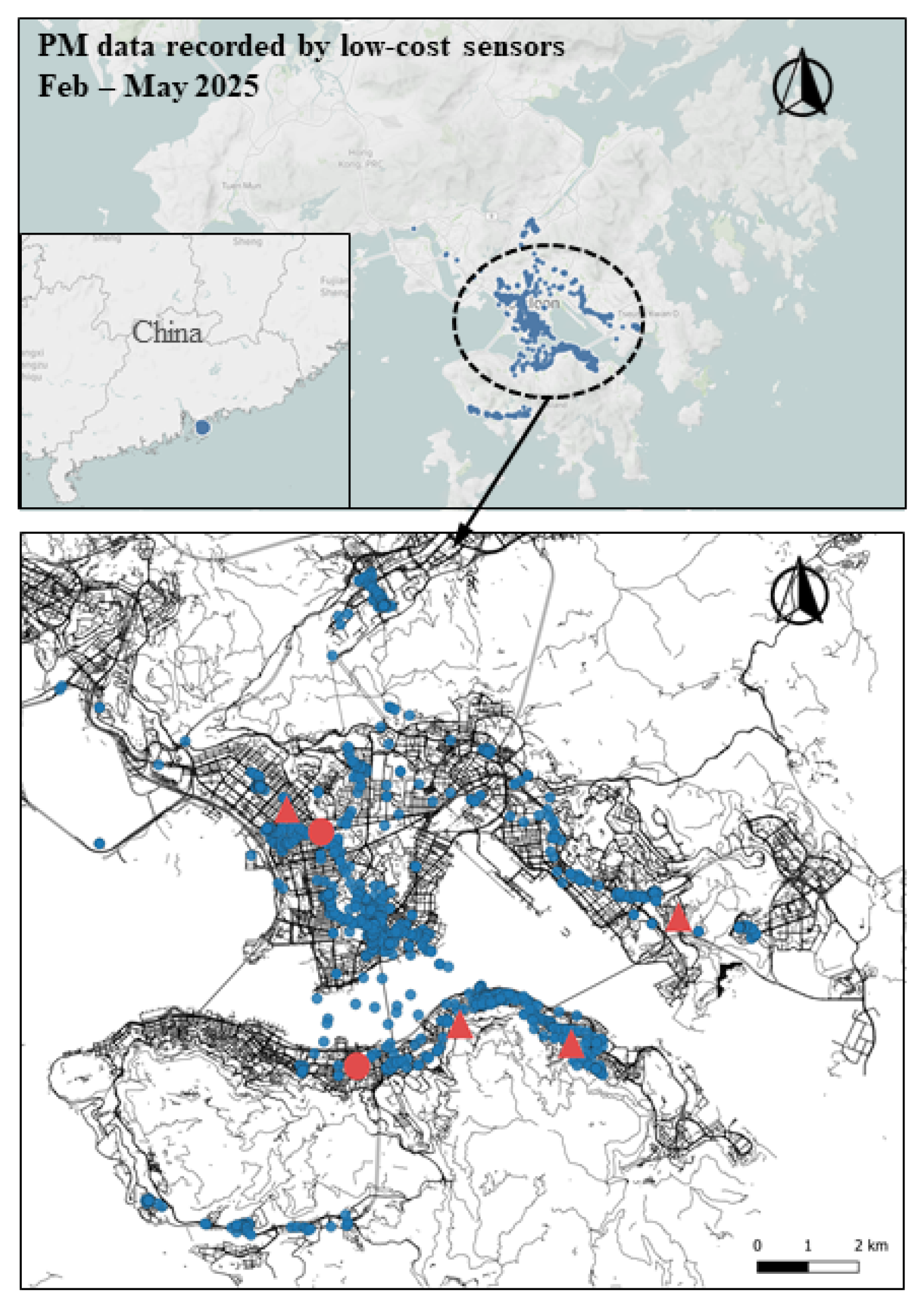
The data collection and measurement were conducted in Hong Kong, a coastal metropolis in southern China. Hong Kong is one of the most densely populated cities in the world, with a population of ~7,500,000. Integrating citizen participation to contribute to building and urban planning, 15 college students were equipped with LWMs for consecutive 48 h measurements. As the sampling interval is one minute, the sample size of 43, 200 min of PM data is enough to conduct the pollution mapping [31]. The study could transform human activities into a dynamic, distributed sampling network by leveraging participants’ daily mobility. All the participants expressed keen interest in monitoring air quality in their ambient micro-environments. They were instructed to take the LWMs with them throughout the day and within 10 feet of their phones to maintain the Bluetooth connection. Figure 3 presents the spatial distribution of measurements across Hong Kong, while the data were presented at different scales. The red circles and triangles represent air quality monitoring stations, with the circles representing roadside stations. The site selection was based on the land-use diversity and socioeconomic variability, including the commercial (Mong Kok), industrial (Kwun Tong), transport hubs (Hung Hom), dense residential (Sham Shui Po), and so on. Most participants resided in urban areas like Kowloon and Hong Kong Island districts. This research was approved by the Ethics Committee of the Hong Kong Polytechnic University (HSEARS20250415002).
Missing values would be interpolated from the closest timeslip to maintain data integrity. Data loss occurred in 4 out of 30 measurements due to user-related errors, such as Bluetooth disconnections and failure to charge monitors. Therefore, 26-day tracking was collected in the database, which is constructed by the ambient temperature, RH, PM1.0, PM2.5, and PM10 concentrations, as well as GPS coordinates. The activity timeline was also integrated with measurements to categorize the indoor-home, outdoor-walking, and hybrid-commuting environments. The following semi-structured interview was also conducted for the detailed cooking and cleaning times. All the data were stripped of identifying information and aggregated based on calendar date and time. The PM concentrations retrieved from the LWMs were plotted using the “ggplot” package in R statistical software (version 4.4.3; R Foundation for Statistical Computing, Vienna, Austria).

3. Results

3.1. Calibration and Performance Analysis

Statistical analysis was conducted to assess the precision and accuracy of the LWMs. Precision represents the stability of PM concentration measurement across the three deployed LWMs, while accuracy refers to the deviation between LWM-recorded data and reference measurements. Raw data would be organized in a dedicated database, removing outliers exceeding the 99th percentile to ensure data quality. The Kolmogorov–Smirnov test revealed the non-normality in the data distribution, prompting the non-parametric Mann–Whitney U test to evaluate differences between measurements. As advertised by the United States Environmental Protection Agency (EPA) air sensor guidebook [32], the coefficient of determination ( R 2 ) and the root mean square error (RMSE) were evaluated in the present study.
R 2 = 1 i = 1 n ( y i y ^ i ) 2 i = 1 n ( y i y ¯ ) 2
R M S E = 1 n i = 1 n ( y i y ^ i ) 2
where y ^ and y refers to the sensor and reference data. The recommended R 2 should exceed 0.70, and the targeted R M S E should be smaller than 7 μg/m3 [33].
All the LWMs with the standard deviation below 1.5 μg/m3 met the acceptability threshold outlined in the USEPA guidelines. The PM concentration traces were close and overlapping, and the difference among the LWMs was near zero. The measurement performance corresponded to the manufacturer’s documented accuracy, confirming the suitability for regression analysis and personal exposure assessment. Previous studies indicated that the multiple linear regression (MLR) model improved the accuracy of raw PM data and extracted pollutant sources [34,35,36]. Therefore, an MLR model (Equation (3)) was implemented to calibrate the PM data recorded by the LWMs, incorporating the RH values [37]. The calibration equation was formulated as follows:
C a l i b r a t e d   P M x = α 1 × r a w P M x + α 2 × R H + β
where α 1 and α 2 indicate the coefficients of the raw PM data and RH, respectively. β is the intercept of the model. The measurement uncertainty used a single-measurement uncertainty analysis [25] and MLR models. The uncertainty values for PM1.0 and PM2.5 measurements were 8.02 μg/m3 and 12.56 μg/m3, respectively.
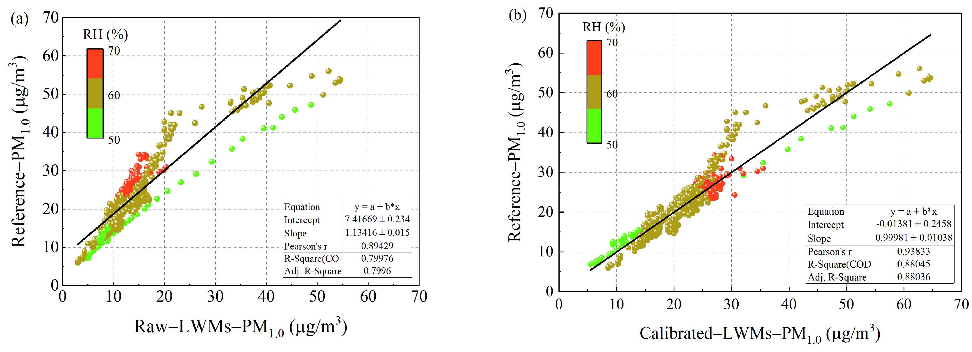
Emerging evidence indicates that the low-cost sensors were only reliable for PM1.0 and PM2.5 quantification but exhibited limited precision for coarse particle measurements [38]. Therefore, the following field calibration focused on the fine particles, PM1.0 and PM2.5. As for the PM1.0, the mean values for the raw and reference data are 13.36 μg/m3 and 22.57 μg/m3, respectively. The raw data recorded by the LWMs underestimated the mass concentration by 40.8% with an RMSE of 2.53 μg/m3 and R 2 of 0.80. From the scatter plot in Figure 4, the impact of RH on the particle mass concentration can be directly noticed. The validation metrics, including RMSE and R 2 , were adopted to evaluate the performance of LWMs. RH as a calibration variable (Equation (4)) can significantly improve the model performance, reducing RMSE from 2.53 μg/m3 to 2.25 μg/m3 and increasing R 2 to 0.88. These parameters reflect the enhanced accuracy of the calibrated model.
C a l i b r a t e d   P M 1.0 = 1.1 × r a w P M 1.0 + 0.66 × R H + ( 33.05 )
The PM2.5 was then calibrated using a similar equation (Equation (5) and Figure 5), with the reduction in RMSE from 3.88 μg/m3 to 3.46 μg/m3. The R 2 has been improved from 0.82 to 0.85. Table 2 presents the calibration results of MLR with accuracy and parameter values. The results were in line with previous FEM field tests by the South Coast Air Quality Management District [39].
C a l i b r a t e d   P M 2.5 = 2.17 × r a w P M 2.5 + 0.64 × R H + ( 34.74 )

3.2. PM Exposure Patterns in Different Environments

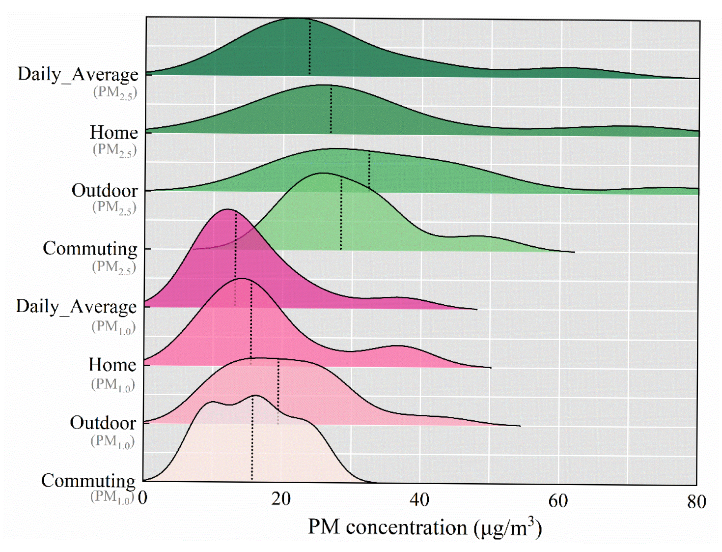
Figure 6 depicts the distribution characteristics of PM1.0 and PM2.5 exposure concentrations across three distinct micro-environments: indoor-home, outdoor-walking, and hybrid-commuting. The ridgeline plot was generated using kernel density estimation [40], and the higher curve referred to the higher occurrence probability. The daily averaged PM2.5 concentration fluctuated between 12 and 64 μg/m3 among the 26-day measurements. The median PM1.0 and PM2.5 exposure concentration (denoted by black dashed lines) were 13.2 μg/m3 and 23.6 μg/m3, respectively. It fulfils the US EPA 24 h air quality standard of 35 μg/m3. However, around 88.5% of the participation measurements exceeded the WHO 24 h guideline of 15 μg/m3. The hybrid-commuting exhibited a narrower, higher concentration distribution (22–33 μg/m3) compared to indoor and outdoor scenarios. The disparity of PM concentrations between subway stations and outdoor road environments may be captured by LWMs as transient peaks during environmental transitions, forming the high-density regions in the concentration distribution. The phenomenon is generally regarded as a short-term exposure event [41,42], indicating that the steady state is not reached before the end of the events. In the present study, commuting generally accounts for around 4–8% of human daily time. One participant’s commuting accounted for 5.5% of his daily time but contributed 11% of his daily PM exposure. The finding aligned with previous investigations [43,44], highlighting the disproportionate impact of transit-related air pollution on individual exposure profiles.

3.3. Spatial Heterogeneity and Source Contribution

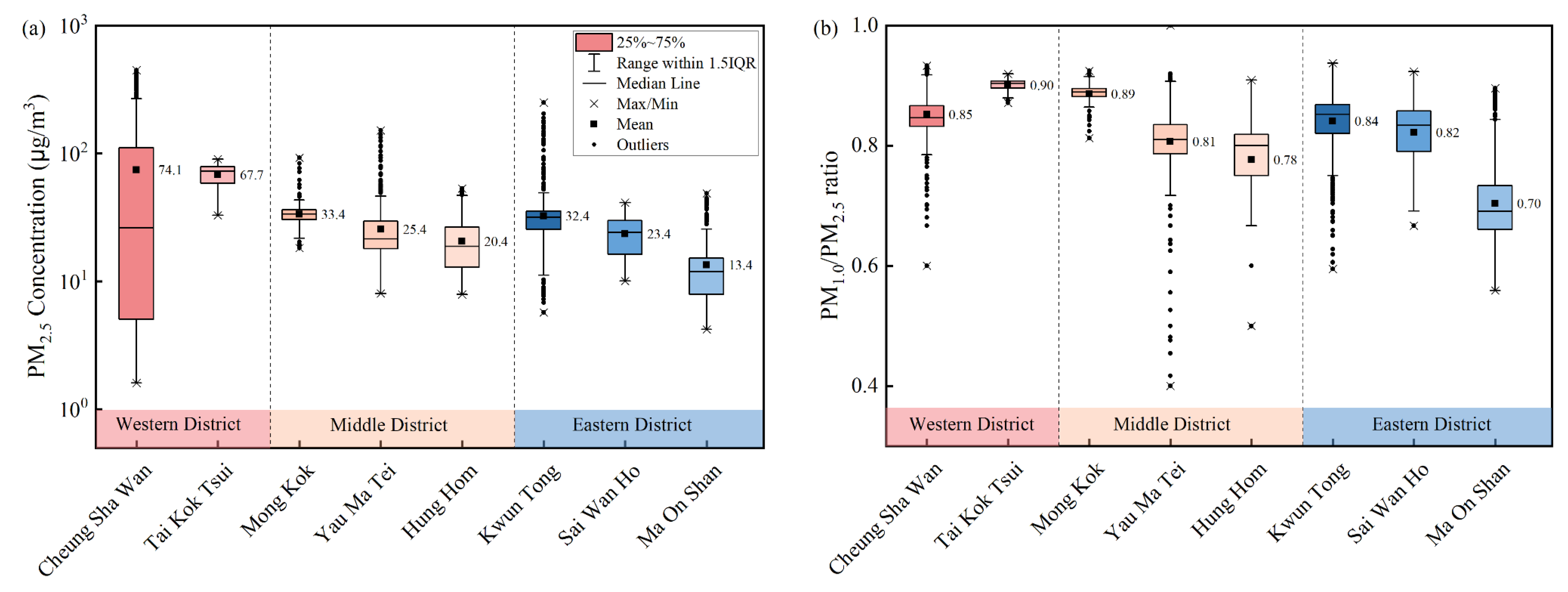
Personal exposure to PM is significantly related to their indoor residential environments and pollution sources [45,46]. Participants in this study spent around 65–80% of their time in residential settings, while the PM2.5 exposure accounted for 42–91% of total personal exposure. Figure 7a presents the box plot chart reporting the indoor PM2.5 concentrations across Hong Kong districts, revealing significant regional diversities. The prevailing south-easterly winds may also influence the urban air quality during the measurement period. The highest PM2.5 concentration was observed in the Western District, with the mean value of 67.7 μg/m3 in Tai Kok Tsui and 74.1 μg/m3 in Cheung Sha Wan. In comparison, the Middle and Eastern District presented a much lower PM2.5 concentration, fluctuating in the range of 13–34 μg/m3. The prevailing south-easterly winds may also influence the urban air quality during the measurement period [47,48]. In the Eastern District, the PM2.5 concentration in Kwun Tong was much higher than in Sai Wan Ho and Ma On Shan during the same measurement period. The dense residents, high-intensity vehicular traffic, and industrial activity are the possible contributing factors [49]. Similar phenomena were also noticed in the Hong Kong roadside investigation about the land-use characteristics [50].
Figure 7b illustrates the PM1.0 and PM2.5 concentration ratio, which can help identify the source contribution characteristics. The ratio below 0.5 indicates that PM2.5 was primarily sourced from the resuspended dust or natural sources. A higher ratio of PM1.0/PM2.5 ( > 0.8 ) represented a higher fraction of fine particles than the coarse ones, sourced from combustion processes (e.g., vehicular emissions). Most measurement sites presented a higher ratio ( > 0.8 ), except the Ma On Shan region. Based on the following semi-structured interview, indoor cooking and traffic emissions were identified as primary PM sources in these high-exposure areas. The lower ratio presented in Ma On Shan can be accounted for by the combination of geographical (sea breezes) and environmental conditions (limited industrial footprint). The study demonstrates the utility of LWMs in understanding the local PM source characteristics, which can help develop evidence-based guidelines for reducing personal exposure to air pollution.

3.4. Hotspot Map and Environmental Justice

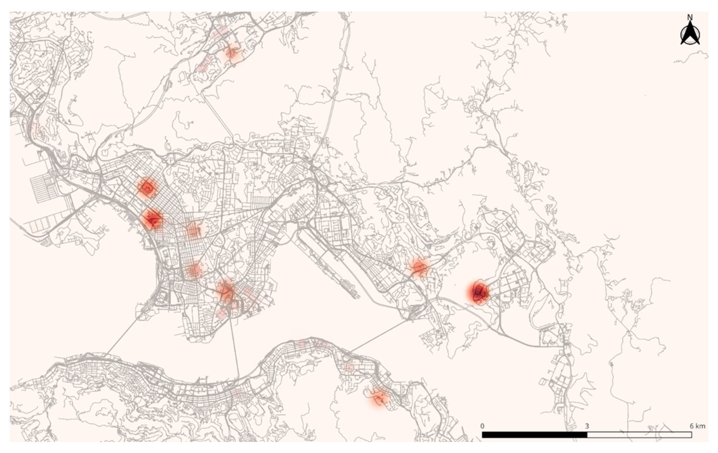
Figure 8 illustrates the hotspot map of PM2.5 concentration across Hong Kong’s different districts, and the map is determined based on the calibrated PM2.5 concentration, GPS data, and open-source software QGIS (version 3.40.7; QGIS Development Team, Zurich, Switzerland). The spatially diverse distribution indicates that the elevated concentration was mainly present in the dense residential (Sham Shui Po), historical industrial (Kwun Tong) areas, major roads, and interchanges. In addition, the meteorological (prevailing southeast wind in spring) and topographic conditions may also disrupt airflow and prolong high PM exposure periods [51]. A computational fluid dynamics simulation has also highlighted the reduced wind speeds and stagnated pollutants in these areas [52,53]. The spatial disparity may also indicate environmental justice concerns and socioeconomic vulnerabilities. Public health records indicate that the aging population and higher rates of respiratory diseases in the Sham Shui Po district amplify susceptibility to pollution [54]. In comparison, the good air quality in Ma On Shan benefits from newer urban planning frameworks, which have stricter emission controls and residential segregation from industrial clusters.

4. Discussion

Global warming, urbanization, and fossil fuel energy consumption have exacerbated air pollution and introduced severe public health issues [55,56]. Accurate and effective air quality monitoring is critical for safeguarding public health. Compared with the traditional and high-maintenance air quality stations, the LWMs have demonstrated their advances in acquiring hyper-localized and high-resolution data. The low-cost sensors require less infrastructure and expertise to deploy [57], which can help to achieve citizen science and geographic coverage. However, deploying low-cost sensors in regulatory measurement involves calibration and performance analysis, especially for their time drift effect and high sensitivity to ambient conditions. Hassani et al. [15] performed the uncertainty quantification analysis of mobile low-cost PM sensors in a Norwegian city, and indicated the necessity of onsite calibration. In addition, the measurement and identification technology (Mie theory) can also lead to different responses to the particle size distribution patterns or particle compositions [58]. Particles in the real world are a heterogeneous mixture of various particle sizes, shapes, refractive indices, and densities, especially for human activities like cooking or candle burning. When the hygroscopic particles are presented in high-humidity environments, they can uptake water and produce a misleading particle size [59]. The employment of LWMs in medical environments should cooperate with the aerodynamic particle sizer, high-speed cameras [60,61], and numerical simulations [62]. Therefore, the present study employed the field co-location in a representative residential environment to calibrate the LWMs. The results indicate the highest performance for the PM1.0, followed by the PM2.5. The linear regression of PM1.0 indicates good agreement with an R2 of 0.88 and an RMSE of 2.25 μg/m3. The R2 and RMSE for PM2.5 were 0.85 and 3.36 μg/m3, respectively. The results are in line with previous FEM field tests and Grimm measurements [39], where the R2 ranged from 0.79 to 0.93. Atmotube Pro has also been widely adopted to monitor air pollution [29,63,64]. As for human exposure patterns, commuting, representing only 5.5% of daily time, contributed disproportionately to total PM exposure (11%). Similar phenomena were also noticed in previous studies [43,44], highlighting the disproportionate impact of transit-related air pollution on individual exposure profiles. Overall, the calibration process can significantly enhance the reliability of LWM-derived data [21,65], thereby strengthening the validity of spatial distribution and source identification in subsequent analyses.
Sampling every location continuously throughout a given geographic area is also an unattainable goal. To address this gap, this study leveraged the mobility of human participants equipped with LWMs, effectively transforming routine activities into a distributed sampling network. By aggregating the spatially diverse measurements over 26 days, it was possible to approximate localized air pollution patterns. The methodology demonstrated that citizen-participated sampling can complement traditional monitoring stations, offering a cost-effective way to map hyper-local pollution gradients. The calibration model of PM concentrations can be transferred to other tropical cities, especially for ambient RH larger than 50%. Re-calibration against local reference instruments can further improve accuracy. The wearing strategy of LWMs on the upper half of the human chest is also recommended, and the sampling location is close to the human breathing zone. The method can provide a basis for the accurate exposure assessment. Through mapping the PM2.5 concentration with the environmental and geospatial data, the residents living in the Sham Shui Po and Kwun Tong areas would be exposed to elevated concentrations. The phenomenon may be accounted for by the proximity to primary pollution sources (industrial activity and traffic emissions), extensive population density, and meteorological trapping. The higher ratio of PM1.0/PM2.5 in Figure 7b and semi-structured interview also indicated the primary particle sources from the traffic and combustion emissions. Sham Shui Po has Hong Kong’s highest population density [66], with plenty of residents living in subdivided units near street-level pollution sources [67]. The mixed-use zoning in Kwun Tong also placed residential areas adjacent to industrial sites. The spatial disparity may also indicate environmental justice concerns and socioeconomic vulnerabilities. The results highlight the necessity of developing prioritized interventions for these regions.
Previous study compared the Aerocet and a Haz–Dust EPAM–5000 particulate monitor (gravimetric technique) [68]. The agreement of PM concentration between the two instruments was over 79%, which was deemed satisfactory. The PM data recorded by the Hong Kong air quality stations were in 1 h resolution [69], and only the qualitative comparisons were conducted on PM2.5 fluctuation ranges (25.2–36.1 μg/m3). The calibration focused on residential settings mainly because humans spend around 80% of their time indoors [70]. However, the sensor calibration across outdoor and transportation settings would enhance the generalizability. Incorporating temperature, atmospheric pressure, and temporal drift in the regression model should also be tested [71], especially using cross-validation or an independent dataset. Future work will include the co-location of LWMs and Aerocet with other government air quality stations to assess agreement and further reduce measurement uncertainty. The PM1.0/PM2.5 ratios and semi-structured interviews were adopted to identify the pollution sources and the detailed cooking and cleaning times. The lack of a solid threshold basis may limit the source identification. Advanced source apportionment methods like the positive matrix factorization have been recommended [72], and future research will consider adopting these methods. In addition, human factors can also induce measurement errors and biases. Yang et al. [73] investigated the effect of sensor wearing strategy on PM concentrations, and the measurement error could even achieve 8.7%. Hassani et al. [15] found that the PM2.5 measurements at different movement speeds also showed high variability. An increase of 1 k m / h could increase the standard deviation by 0.03 μg/m3. The present study suggested a wearing strategy on the upper half of the human chest, near the breathing zone. The engagement of citizen participation plays a critical part in providing the valuable spatial variability of air quality at urban levels. Future studies should consider the effect of movement routes and velocity.

5. Conclusions

The present study has leveraged the mobility of human participants equipped with LWMs, transforming routine activities into a distributed sampling network. Integrating citizen science and LWMs can provide valuable data about the hyper-localized air pollution and personal exposure.
The scientific reliability of LWMs has been evaluated through field co-location in residential settings, calibrated by a gravimetrically pre-calibrated aerosol analyzer. The performance of LWMs had been significantly improved by the MLR model adjusted for the moderated RH range (50–70%) in tropical regions. The R2 of PM1.0 and PM2.5 had been increased to over 0.85 after calibration, along with the reduced RMSE of 2.25 and 3.46 μg/m3, respectively. All the metrics fall within the acceptability threshold outlined in the USEPA guidelines. These results support preliminary community-level monitoring, and broader validation across seasons and scenarios remains necessary.
Participant exposure patterns were analyzed across indoor-home, outdoor-walking, and commuting micro-environments, with the median PM1.0 (13.2 μg/m3) and PM2.5 (23.6 μg/m3. Commuting generally constituted a small fraction of daily time but contributed disproportionately to 11% of personal PM exposure. The targeted intervention for transit-related air pollution is quite critical for urban development.
Spatial analysis reveals district-level disparities, with residential PM2.5 exposure accounting for 42–91% of total personal exposure. Elevated PM concentrations were presented in the dense residential (Sham Shui Po), historical industrial (Kwun Tong) areas, and major roads and highway system interchanges. PM1.0/PM2.5 ratios and semi-structured interviews indicates that the indoor cooking and traffic emissions were the primary PM sources in these hotspots. Building ventilation retrofits can help reduce residential exposure. Future research should further integrate border validation, long-term monitoring, and advanced source apportionment methods to provide empirical evidence for building and urban planning.

Author Contributions

Conceptualization, X.L. and C.M.M.; methodology, X.L.; formal analysis, X.L. and Y.D.; investigation, X.L. and K.W.M.; resources, H.M.W.; writing—original draft preparation, X.L.; writing—review and editing, C.M.M. and K.W.M.; supervision, C.M.M.; project administration, C.M.M. and H.M.W.; funding acquisition, C.M.M. All authors have read and agreed to the published version of the manuscript.

Funding

This research was funded by Postdoc Matching Fund Scheme of Hong Kong Polytechnic University (1-W32R).

Data Availability Statement

The original contributions presented in this study are included in the article. Further inquiries can be directed to the corresponding author(s).

Conflicts of Interest

The authors declare no conflicts of interest. The funders had no role in the design of the study; in the collection, analyses, or interpretation of data; in the writing of the manuscript; or in the decision to publish the results.

References

  1. Thurston, G.D.; Kipen, H.; Annesi-Maesano, I.; Balmes, J.; Brook, R.D.; Cromar, K.; De Matteis, S.; Forastiere, F.; Forsberg, B.; Frampton, M.W.; et al. A joint ERS/ATS policy statement: What constitutes an adverse health effect of air pollution? An analytical framework. Eur. Respir. J. 2017, 49, 1600419. [Google Scholar] [CrossRef]
  2. Manu, S.; Rysanek, A. A Co-Location Study of 87 Low-Cost Environmental Monitors: Assessing Outliers, Variability, and Uncertainty. Buildings 2024, 14, 2965. [Google Scholar] [CrossRef]
  3. Agency, E.E. Europe’s Air Quality Status 2023. Available online: https://www.eea.europa.eu/en/analysis/publications/europes-air-quality-status-2023 (accessed on 25 August 2025).
  4. Pai, S.J.; Carter, T.S.; Heald, C.L.; Kroll, J.H. Updated World Health Organization Air Quality Guidelines Highlight the Importance of Non-anthropogenic PM(2.5). Environ. Sci. Technol. Lett. 2022, 9, 501–506. [Google Scholar] [CrossRef]
  5. Sigsgaard, T.; Hoffmann, B. Assessing the health burden from air pollution. Science 2024, 384, 33–34. [Google Scholar] [CrossRef]
  6. Nie, T.; Zhang, G.F.; Sun, Y.N.; Wang, W.H.; Wang, T.N.; Duan, H.Y. Effects of Indoor Air Quality on Human Physiological Impact: A Review. Buildings 2025, 15, 1296. [Google Scholar] [CrossRef]
  7. Peters, T.; Zhen, C. Evaluating indoor air quality monitoring devices for healthy homes. Buildings 2023, 14, 102. [Google Scholar] [CrossRef]
  8. Heaney, A.; Stowell, J.D.; Liu, J.C.; Basu, R.; Marlier, M.; Kinney, P. Impacts of Fine Particulate Matter from Wildfire Smoke on Respiratory and Cardiovascular Health in California. Geohealth 2022, 6, e2021GH000578. [Google Scholar] [CrossRef]
  9. Sun, C.J.; Wang, Q.H.; Zhang, J.L.; Zou, Z.J.; He, X.W.; Niu, J.L.; Wang, H.D.; Su, C.X.; Lu, R.C.; Huang, B.J.; et al. Cancer risk and sick building syndrome in different regions of China: Potential hazard from particulate matter and phthalate pollutants. Sustain. Cities Soc. 2025, 124, 106297. [Google Scholar] [CrossRef]
  10. Zhang, Y.Q.; Wei, J.; Chen, S.R.; Benmarhnia, T.; Zhang, K.; Wang, X.W.; Deng, X.L.; Gu, H.G.; Lin, Z.Q.; Qu, Y.J.; et al. Individual and mixed associations between fine particulate matter components and hospital admissions for hypertension: Insights from a large-scale South Chinese cohort study. Sustain. Cities Soc. 2025, 124, 106293. [Google Scholar] [CrossRef]
  11. Noble, C.A.; Vanderpool, R.W.; Peters, T.M.; McElroy, F.F.; Gemmill, D.B.; Wiener, R.W. Federal reference and equivalent methods for measuring fine particulate matter. Aerosol Sci. Technol. 2001, 34, 457–464. [Google Scholar] [CrossRef]
  12. Morawska, L.; Asbach, C.; Patel, H. Application of PM low-cost sensors for indoor air quality compliance monitoring. Aerosol Sci. Technol. 2025, 1–11. [Google Scholar] [CrossRef]
  13. Zhang, H.; Evangelopoulos, D.; Wood, D.; Chatzidiakou, L.; Varaden, D.; Quint, J.; de Nazelle, A.; Walton, H.; Katsouyanni, K.; Barratt, B. Estimating exposure to pollutants generated from indoor and outdoor sources within vulnerable populations using personal air quality monitors: A London case study. Environ. Int. 2025, 198, 109431. [Google Scholar] [CrossRef] [PubMed]
  14. Vishal; Sharma, M.; Jain, S. Unmanned aerial vehicles and low-cost sensors for air quality monitoring: A comprehensive review of applications across diverse emission sources. Sustain. Cities Soc. 2025, 127, 106409. [Google Scholar] [CrossRef]
  15. Hassani, A.; Castell, N.; Watne, A.K.; Schneider, P. Citizen-operated mobile low-cost sensors for urban PM monitoring: Field calibration, uncertainty estimation, and application. Sustain. Cities Soc. 2023, 95, 104607. [Google Scholar] [CrossRef]
  16. Hankey, S.; Sforza, P.; Pierson, M. Using Mobile Monitoring to Develop Hourly Empirical Models of Particulate Air Pollution in a Rural Appalachian Community. Environ. Sci. Technol. 2019, 53, 4305–4315. [Google Scholar] [CrossRef]
  17. Mueller, M.D.; Hasenfratz, D.; Saukh, O.; Fierz, M.; Hueglin, C. Statistical modelling of particle number concentration in Zurich at high spatio-temporal resolution utilizing data from a mobile sensor network. Atmos. Environ. 2016, 126, 171–181. [Google Scholar] [CrossRef]
  18. Sun, Y.; Brimblecombe, P.; Wei, P.; Duan, Y.; Pan, J.; Liu, Q.; Fu, Q.; Peng, Z.; Xu, S.; Wang, Y.; et al. High Resolution On-Road Air Pollution Using a Large Taxi-Based Mobile Sensor Network. Sensors 2022, 22, 6005. [Google Scholar] [CrossRef]
  19. Zheng, T.S.; Bergin, M.H.; Johnson, K.K.; Tripathi, S.N.; Shirodkar, S.; Landis, M.S.; Sutaria, R.; Carlson, D.E. Field evaluation of low-cost particulate matter sensors in high-and low-concentration environments. Atmos. Meas. Tech. 2018, 11, 4823–4846. [Google Scholar] [CrossRef]
  20. Badura, M.; Batog, P.; Drzeniecka-Osiadacz, A.; Modzel, P. Evaluation of Low-Cost Sensors for Ambient PM2.5 Monitoring. J. Sensors 2018, 2018, 5096540. [Google Scholar] [CrossRef]
  21. Hofman, J.; Lazarov, B.; Stroobants, C.; Elst, E.; Smets, I.; Van Poppel, M. Portable Sensors for Dynamic Exposure Assessments in Urban Environments: State of the Science. Sensors 2024, 24, 5653. [Google Scholar] [CrossRef]
  22. Li, X.; Wei, Y.; Zhang, J.; Jin, P. Design and analysis of an active daylight harvesting system for building. Renew. Energy 2019, 139, 670–678. [Google Scholar] [CrossRef]
  23. Cheriyan, D.; Choi, J.H. Estimation of particulate matter exposure to construction workers using low-cost dust sensors. Sustain. Cities Soc. 2020, 59, 102197. [Google Scholar] [CrossRef]
  24. Ruiter, S.; Bard, D.; Ben Jeddi, H.; Saunders, J.; Snawder, J.; Warren, N.; Gorce, J.P.; Cauda, E.; Kuijpers, E.; Pronk, A. Exposure Monitoring Strategies for Applying Low-Cost PM Sensors to Assess Flour Dust in Industrial Bakeries. Ann. Work Expo. Health 2023, 67, 379–391. [Google Scholar] [CrossRef] [PubMed]
  25. Kang, Y.; Aye, L.; Ngo, T.D.; Zhou, J. Performance evaluation of low-cost air quality sensors: A review. Sci. Total Environ. 2022, 818, 151769. [Google Scholar] [CrossRef] [PubMed]
  26. Li, X.; Mak, C.M.; Ai, Z.; Wong, H.M. Airborne transmission of exhaled pollutants during short-term events: Quantitatively assessing inhalation monitor points. Build. Environ. 2022, 223, 109487. [Google Scholar] [CrossRef]
  27. Chiliński, M.T.; Broda, M.; Nurowska, K.; Markowicz, K. The Near-Surface Vertical Variability of Aerosol Single-Scattering Properties over Warsaw: Case Study. Aerosol Air Qual. Res. 2025, 25, 14. [Google Scholar] [CrossRef]
  28. Pérez, A.P.; Fernández, E.I.; Shah, S.M.A.; Casado-Mansilla, D.; Valera, A.J.J.; López-De-Ipiña, D. Performance assessment of wearable atmotube pro sensor for air quality citizen science applications. In Proceedings of the 2024 9th International Conference on Smart and Sustainable Technologies (SpliTech), Bol and Split, Croatia, 25–28 June 2024; pp. 1–6. [Google Scholar] [CrossRef]
  29. Shittu, A.; Pringle, K.; Arnold, S.; Pope, R.; Graham, A.; Reddington, C.; Rigby, R.; McQuaid, J. Performance Evaluation of Atmotube Pro sensors for Air Quality Measurements. EGUsphere 2024, 2024, 1–17. [Google Scholar] [CrossRef]
  30. Steinle, S.; Reis, S.; Sabel, C.E.; Semple, S.; Twigg, M.M.; Braban, C.F.; Leeson, S.R.; Heal, M.R.; Harrison, D.; Lin, C. Personal exposure monitoring of PM2. 5 in indoor and outdoor microenvironments. Sci. Total Environ. 2015, 508, 383–394. [Google Scholar] [CrossRef] [PubMed]
  31. Sloan, C.D.; Philipp, T.J.; Bradshaw, R.K.; Chronister, S.; Barber, W.B.; Johnston, J.D. Applications of GPS-tracked personal and fixed-location PM2.5 continuous exposure monitoring. J. Air Waste Manag. 2016, 66, 53–65. [Google Scholar] [CrossRef]
  32. Clements, A.; Duvall, R.; Greene, D.; Dye, T. The Enhanced Air Sensor Guidebook. Available online: https://www.epa.gov/air-sensor-toolbox/how-use-air-sensors-air-sensor-guidebook (accessed on 29 August 2025).
  33. Zimmerman, N. Tutorial: Guidelines for implementing low-cost sensor networks for aerosol monitoring. J. Aerosol. Sci. 2022, 159, 105872. [Google Scholar] [CrossRef]
  34. Lee, H.; Kang, J.; Kim, S.; Im, Y.; Yoo, S.; Lee, D. Long-Term Evaluation and Calibration of Low-Cost Particulate Matter (PM) Sensor. Sensors 2020, 20, 3617. [Google Scholar] [CrossRef]
  35. Romero, Y.; Velasquez, R.M.A.; Noel, J. Development of a multiple regression model to calibrate a low-cost sensor considering reference measurements and meteorological parameters. Environ. Monit. Assess. 2020, 192, 498. [Google Scholar] [CrossRef] [PubMed]
  36. Stavroulas, I.; Grivas, G.; Michalopoulos, P.; Liakakou, E.; Bougiatioti, A.; Kalkavouras, P.; Fameli, K.M.; Hatzianastassiou, N.; Mihalopoulos, N.; Gerasopoulos, E. Field Evaluation of Low-Cost PM Sensors (Purple Air PA-II) Under Variable Urban Air Quality Conditions, in Greece. Atmosphere 2020, 11, 926. [Google Scholar] [CrossRef]
  37. Mai, C.; Wang, Z.; Chen, L.; Huang, Y.; Li, M.; Shirazi, A.; Altaee, A.; Zhou, J.L. Field-based Calibration and Operation of Low-Cost Sensors for Particulate Matter by Linear and Nonlinear Methods. Atmos. Pollut. Res. 2025, 16, 102676. [Google Scholar] [CrossRef]
  38. Molina Rueda, E.; Carter, E.; L’Orange, C.; Quinn, C.; Volckens, J. Size-Resolved Field Performance of Low-Cost Sensors for Particulate Matter Air Pollution. Environ. Sci. Technol. Lett. 2023, 10, 247–253. [Google Scholar] [CrossRef]
  39. Air Quality Sensor Performance Evaluation Center Evaluation Summary: Atmotube Pro. Available online: http://www.aqmd.gov/docs/default-source/aq-spec/summary/atmotube-pro---summary-report.pdf?sfvrsn=8 (accessed on 24 August 2025).
  40. Cox, N.J. Kernel estimation as a basic tool for geomorphological data analysis. Earth Surf. Proc. Land. 2007, 32, 1902–1912. [Google Scholar] [CrossRef]
  41. Kloog, I.; Ridgway, B.; Koutrakis, P.; Coull, B.A.; Schwartz, J.D. Long- and short-term exposure to PM2.5 and mortality: Using novel exposure models. Epidemiology 2013, 24, 555–561. [Google Scholar] [CrossRef] [PubMed]
  42. Li, X.; Ai, Z.; Ye, J.; Mak, C.M.; Wong, H.M. Airborne transmission during short-term events: Direct route over indirect route. Build. Simul. 2022, 15, 2097–2110. [Google Scholar] [CrossRef]
  43. Chaney, R.A.; Sloan, C.D.; Cooper, V.C.; Robinson, D.R.; Hendrickson, N.R.; McCord, T.A.; Johnston, J.D. Personal exposure to fine particulate air pollution while commuting: An examination of six transport modes on an urban arterial roadway. PLoS ONE 2017, 12, e0188053. [Google Scholar] [CrossRef]
  44. Ramel-Delobel, M.; Peruzzi, C.; Coudon, T.; De Vito, S.; Fattoruso, G.; Praud, D.; Fervers, B.; Salizzoni, P. Exposure to airborne particulate matter during commuting using portable sensors: Effects of transport modes in a French metropolis study case. J. Environ. Manag. 2024, 365, 121400. [Google Scholar] [CrossRef]
  45. Tham, K.W. Indoor air quality and its effects on humans—A review of challenges and developments in the last 30 years. Energy Build. 2016, 130, 637–650. [Google Scholar] [CrossRef]
  46. Li, X.; Mak, C.M.; Ai, Z.; Ma, K.W.; Wong, H.M. Cross-infection risk assessment in dental clinic: Numerical investigation of emitted droplets during different atomization procedures. J. Build. Eng. 2023, 75, 106961. [Google Scholar] [CrossRef]
  47. Cheng, S.; Lam, K.-c. An analysis of winds affecting air pollution concentrations in Hong Kong. Atmos. Environ. 1998, 32, 2559–2567. [Google Scholar] [CrossRef]
  48. Huang, X.-F.; Yu, J.Z.; Yuan, Z.; Lau, A.K.; Louie, P.K. Source analysis of high particulate matter days in Hong Kong. Atmos. Environ. 2009, 43, 1196–1203. [Google Scholar] [CrossRef]
  49. Ho, K.; Lee, S.; Jimmy, C.Y.; Zou, S.; Fung, K. Carbonaceous characteristics of atmospheric particulate matter in Hong Kong. Sci. Total Environ. 2002, 300, 59–67. [Google Scholar] [CrossRef]
  50. Chan, L.; Kwok, W.; Chan, C. Study of Participate at the Roadside Microenvironment in Different Land Use Areas in Hong Kong. WIT Trans. Ecol. Environ. 2024, 28, 9. [Google Scholar] [CrossRef]
  51. Leung, D.M.; Tai, A.P.; Mickley, L.J.; Moch, J.M.; Van Donkelaar, A.; Shen, L.; Martin, R.V. Synoptic meteorological modes of variability for fine particulate matter (PM 2.5) air quality in major metropolitan regions of China. Atmos. Chem. Phys. 2018, 18, 6733–6748. [Google Scholar] [CrossRef]
  52. Dai, Y.W.; Mak, C.M.; Ai, Z.T.; Hang, J. Evaluation of computational and physical parameters influencing CFD simulations of pollutant dispersion in building arrays. Build. Environ. 2018, 137, 90–107. [Google Scholar] [CrossRef]
  53. Dai, Y.W.; Tu, W.L.; Zhang, X.Y.; Li, J.Z.; Yue, X.P.; Wang, H.D. Dynamic wind patterns and indoor/outdoor pollutant dispersion in the simplified building array: Statistical and spectral analyses from scaled outdoor experiments. Build. Environ. 2025, 276, 112861. [Google Scholar] [CrossRef]
  54. Air Science Group, Environmental Protection Department. Air Quality in Hong Kong 2012. Available online: https://www.aqhi.gov.hk/common/api_history/english/report/files/AQR2012e_final.pdf (accessed on 29 August 2025).
  55. Apte, J.S.; Manchanda, C. High-resolution urban air pollution mapping. Science 2024, 385, 380–385. [Google Scholar] [CrossRef]
  56. Li, X.J.; Mak, C.M.; Xue, P.; Xue, R.; Wong, H.M. Unraveling the applicability and thermal performance of PCM-impregnated wood in personalized comfort systems: Thermal manikin verification. Energy Build. 2025, 344, 116028. [Google Scholar] [CrossRef]
  57. Anik, S.M.H.; Gao, X.H.; Meng, N.R.; Agee, P.P.; McCoy, A. A cost-effective, scalable, and portable IoT data infrastructure for indoor environment sensing. J. Build. Eng. 2022, 49, 104027. [Google Scholar] [CrossRef]
  58. Ouimette, J.; Arnott, W.P.; Laven, P.; Whitwell, R.; Radhakrishnan, N.; Dhaniyala, S.; Sandink, M.; Tryner, J.; Volckens, J. Fundamentals of low-cost aerosol sensor design and operation. Aerosol Sci. Tech. 2024, 58, 1–15. [Google Scholar] [CrossRef]
  59. Tang, M.J.; Chan, C.K.; Li, Y.J.; Su, H.; Ma, Q.X.; Wu, Z.J.; Zhang, G.H.; Wang, Z.; Ge, M.F.; Hu, M.; et al. A review of experimental techniques for aerosol hygroscopicity studies. Atmos. Chem. Phys. 2019, 19, 12631–12686. [Google Scholar] [CrossRef]
  60. Li, X.; Mak, C.M.; Ai, Z.; Ma, K.W.; Wong, H.M. Propagation and evaporation of contaminated droplets, emission and exposure in surgery environments revealed by laser visualization and numerical characterization. J. Hazard. Mater. 2024, 477, 135338. [Google Scholar] [CrossRef] [PubMed]
  61. Li, X.; Mak, C.M.; Ma, K.W.; Wong, H.M. Evaluating flow-field and expelled droplets in the mockup dental clinic during the COVID-19 pandemic. Phys. Fluids 2021, 33, 047111. [Google Scholar] [CrossRef]
  62. Li, X.; Mak, C.M.; Ma, K.W.; Wong, H.M. Large eddy simulation study on dental spray dynamics and infection during ultrasonic atomization. J. Build. Eng. 2025, 103, 112164. [Google Scholar] [CrossRef]
  63. Shittu, A.I.; Pope, R.J.; Pringle, K.J.; Arnold, S.R.; Graham, A.M.; Sideeq, H.O.; Ana, G.R.; McQuaid, J.B. Quantifying Residential Particulate Pollution and Human Exposure in Ibadan, Nigeria, Using Low-Cost Sensors. Aerosol Air Qual. Res. 2025, 25, 44. [Google Scholar] [CrossRef]
  64. Lanza, K.; Allison, B.; Chen, B.; Wilson, P.S.; Hunt, E.T.; Burford, K.G.; Zhang, Y.; Ganzar, L.A.; Keitt, T.H. Ambient environmental exposures while cycling on a vegetated trail versus the road. Urban Clim. 2025, 61, 102429. [Google Scholar] [CrossRef]
  65. Feng, Z.; Zheng, L.; Ren, B.; Liu, D.; Huang, J.; Xue, N. Feasibility of low-cost particulate matter sensors for long-term environmental monitoring: Field evaluation and calibration. Sci. Total Environ. 2024, 945, 174089. [Google Scholar] [CrossRef] [PubMed]
  66. Tang, W.S.; Lee, J.W.; Hui, T.W.; Yip, M.K. The “Urban density” question in Hong Kong: From absolute space to social processes. City Cult. Soc. 2019, 17, 46–53. [Google Scholar] [CrossRef]
  67. Tan, Y.Y.; Song, J.S.; Yu, L.; Bai, Y.X.; Zhang, J.F.; Chan, M.H.; van Ameijde, J. The Mechanism of Street Markets Fostering Supportive Communities in Old Urban Districts: A Case Study of Sham Shui Po, Hong Kong. Land 2024, 13, 289. [Google Scholar] [CrossRef]
  68. McNabola, A.; McCreddin, A.; Gill, L.W.; Broderick, B.M. Analysis of the relationship between urban background air pollution concentrations and the personal exposure of office workers in Dublin, Ireland, using baseline separation techniques. Atmos. Pollut. Res. 2011, 2, 80–88. [Google Scholar] [CrossRef]
  69. Environmental Protection Department, The Government of the Hong Kong Special Administrative Region. Past Air Quality, Mong Kok, Pollutant Concentration. Available online: https://www.aqhi.gov.hk/en/aqhi/past-24-hours-aqhi.html?mid=17 (accessed on 24 August 2025).
  70. Zhong, X.; Zhang, Z.; Wu, W.; Zhang, R. Estimating space-cooling energy consumption and indoor PM2. 5 exposure across Hong Kong using a city-representative housing stock model. Buildings 2022, 12, 1414. [Google Scholar] [CrossRef]
  71. Cui, H.; Zhang, L.; Li, W.; Yuan, Z.; Wu, M.; Wang, C.; Ma, J.; Li, Y. A new calibration system for low-cost sensor network in air pollution monitoring. Atmos. Pollut. Res. 2021, 12, 101049. [Google Scholar] [CrossRef]
  72. Bousiotis, D.; Damayanti, S.; Baruah, A.; Bigi, A.; Beddows, D.C.; Harrison, R.M.; Pope, F.D. Pinpointing sources of pollution using citizen science and hyperlocal low-cost mobile source apportionment. Environ. Int. 2024, 193, 109069. [Google Scholar] [CrossRef] [PubMed]
  73. Yang, W.; Zhao, B. A real-time personal PM2. 5 exposure monitoring system and its application for college students. Build. Simul. 2024, 17, 1531–1539. [Google Scholar] [CrossRef]
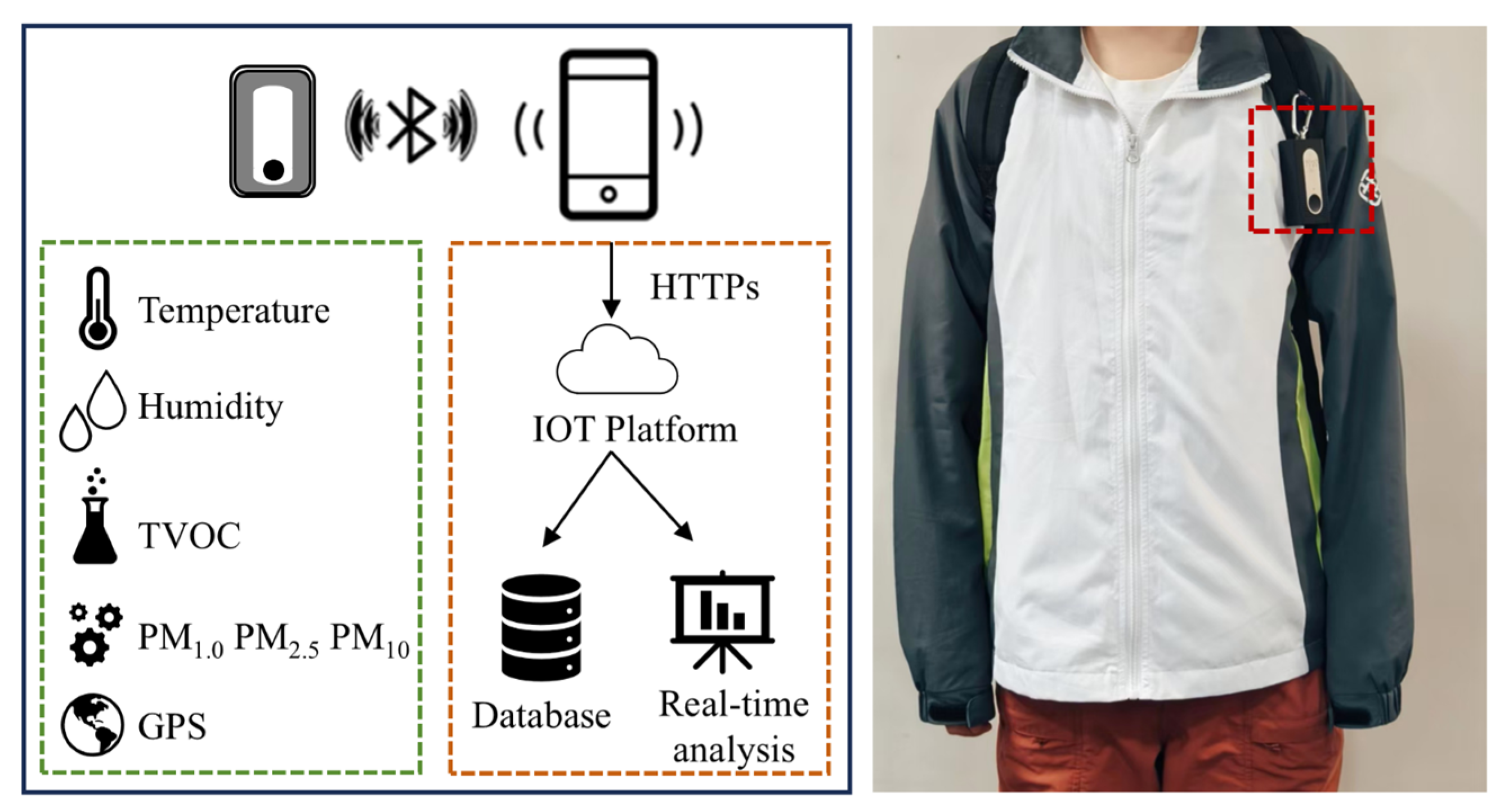
Figure 1. Schematic diagram of LWMs and wearing strategy for mobile data collection in the red dotted box.
Buildings 15 03131 g001
Figure 2. Research flow chart of the present research.
Buildings 15 03131 g002
Figure 3. Spatial distribution of the LWM measurement (blue point) in Hong Kong and corresponding air quality stations in red triangles. Red circles refer to the roadside stations.
Buildings 15 03131 g003
Figure 4. Scatter plot for PM1.0 recorded by LWMs against reference instrument as a function of RH: (a) raw and (b) calibrated data.
Buildings 15 03131 g004
Figure 5. Scatter plot for PM2.5 recorded by LWMs against reference instrument as a function of RH: (b) raw and (b) calibrated data.
Buildings 15 03131 g005
Figure 6. Ridgeline plot of the daily average PM exposure concentration in indoor-home, outdoor-walking, and hybrid-commuting micro-environments: black dashed lines indicating the median concentration values.
Buildings 15 03131 g006
Figure 7. The box plot chart reporting the spatial heterogeneity of residential PM concentration in different districts of Hong Kong: (a) the PM2.5 concentration distribution; (b) PM1.0/ PM2.5 ratios for source contribution analysis.
Buildings 15 03131 g007
Figure 8. Hotspot map of calibrated PM2.5 concentration in different districts of Hong Kong.
Buildings 15 03131 g008
Table 1. Measurement and sensor characteristics.
SensorParameterRangeAccuracy
Bosch BME280Temperature−40 to 85 °C±0.5 °C
Bosch BME280Humidity0 to 100%±3% RH
Bosch BME280Pressure300 to 1100 hPa±1.7 hPa
Sensirion SPS30PM1.0, PM2.5, PM100 to 1000 μg/m30 to 100 ± 10 μg/m3
100 to 1000 ± 10% μg/m3
Sensirion SGPC3TVOC0 to 60,000 ppb±15%
Table 2. Calibration results of MLR model.
MLR ModelAccuracy/PerformanceParameter Values
R2RMSE α 1 α 2 β
PM1.00.882.25 μg/m31.10.66−33.05
PM2.50.853.46 μg/m32.170.64−34.74
Disclaimer/Publisher’s Note: The statements, opinions and data contained in all publications are solely those of the individual author(s) and contributor(s) and not of MDPI and/or the editor(s). MDPI and/or the editor(s) disclaim responsibility for any injury to people or property resulting from any ideas, methods, instructions or products referred to in the content.