Efficient Swell Risk Prediction for Building Design Using a Domain-Guided Machine Learning Model

Abstract

Expansive clays damage the foundations, slabs, and utilities of low- and mid-rise buildings, threatening daily operations and incurring billions of dollars in costs globally. This study pioneers a domain-informed machine learning framework, coupled with a collinearity-aware feature selection strategy, to predict soil swell potential solely from routine index properties. Following hard-limit filtering and Unified Soil Classification System (USCS) screening, 291 valid samples were extracted from a public dataset of 395 cases. A random forest benchmark model was developed using five correlated features, and a multicollinearity analysis, as indicated by the variance inflation factor, revealed exact linear dependence among the Atterberg limits. A parsimonious two-variable model, based solely on plasticity index (PI) and clay fraction (C), was retained. On an 80:20 stratified hold-out set, this simplified model reduced root mean square error (RMSE) from 9.0% to 6.8% and maximum residuals from 42% to 16%. Bootstrap analysis confirmed a median RMSE of 7.5% with stable 95% prediction intervals. Shapley Additive Explanations (SHAP) analysis revealed that PI accounted for approximately 75% of the model’s influence, highlighting the critical swell surge beyond PI ≈ 55%. This work introduces a rule-based cleaning pipeline and collinearity-aware feature selection to derive a robust, two-variable model balancing accuracy and interpretability, a lightweight, interpretable tool for foundation design, GIS zoning, and BIM workflows.

1. Introduction

Expansive clays present a significant geotechnical hazard for the built environment due to their tendency to swell upon wetting and shrink upon drying [1,2,3]. These volumetric changes can lead to substantial ground movement, causing structural distress to shallow foundations, floor slabs, retaining walls, and underground utilities [4,5]. In regions characterized by arid and semi-arid climates, where seasonal or event-driven fluctuations in moisture are typical, expansive soils are a leading cause of differential settlement and long-term damage to low- and mid-rise buildings [5,6]. The global economic burden from expansive soil-related damage is estimated in the billions of dollars annually, with repairs frequently involving underpinning, slab lifting, or complete structural rehabilitation [7,8].

For building engineers, designers, and construction managers, the early identification and management of expansive soils is therefore critical [9,10]. Swelling behavior can compromise not only the initial construction integrity but also the long-term performance, safety, and serviceability of buildings [11,12]. Despite the seriousness of this threat, expansive soils are frequently underassessed in early-stage design due to the cost and complexity of traditional testing methods [11]. Laboratory procedures such as oedometer swell tests or swell pressure tests are accurate but time-consuming, expensive, and impractical for broad site coverage or early-phase feasibility studies [1]. These constraints limit their utility in the fast-paced workflows of modern construction and infrastructure planning.

In light of these limitations, there is growing interest in geotechnical and building engineering research in applying data-driven methods as potential alternatives to conventional swell assessment techniques [7,13,14,15,16]. Among these, ML models have shown promise in predicting soil swell behavior from basic index properties, such as the plasticity index, liquid limit, and clay fraction, which are routinely measured in standard geotechnical investigations [8,17,18,19]. By learning predictive relationships from historical data, ML models can reduce the reliance on slow laboratory tests and provide preliminary risk screening at the planning and design stages [17,18].

However, many existing ML models for swell prediction are hindered by limitations that restrict their practical value in the building domain. Common issues include small or region-specific datasets, overfitting due to high feature redundancy, and a lack of transparency in model predictions. In particular, models that use correlated geotechnical parameters without accounting for multicollinearity can yield unstable or misleading outputs [19,20]. Additionally, most models do not provide uncertainty bounds or insight into the reasoning behind a given prediction, reducing their trustworthiness in design workflows [21,22].

To make ML a reliable tool for building-related geotechnical prediction, domain knowledge must be explicitly integrated into the modeling process. A domain-informed ML approach involves applying geotechnical expertise at every stage, from data preprocessing and feature selection to model evaluation and interpretation [23,24]. For instance, rather than using all available index properties indiscriminately, this study emphasizes the role of plasticity index and clay content, parameters with established links to swelling behavior and physical soil mechanisms [25,26]. Reducing inputs to the most influential and geotechnically sound variables improves model stability and interpretability [14,27].

Interpretability is especially important for practical building applications, where design engineers and construction professionals must understand the rationale behind a risk assessment. To support this, explainable techniques, including SHAP and partial dependence plots (PDPs), are employed. These tools clarify how each input feature contributes to a prediction, enabling the model to function as a transparent decision-support system rather than a black box [28,29]. SHAP values indicate which features, such as high plasticity or elevated clay fraction, drive the model’s swell predictions, while PDPs visualize these relationships across a realistic range of soil conditions [18,30]. Comparable progress has been reported for seismic problems; Pistolesi et al. [31] demonstrated that an explainable AI model can predict failure mechanisms and critical seismic acceleration of flexible retaining walls in milliseconds while still providing SHAP-based insights.

This study also emphasizes the importance of predictive uncertainty. Using bootstrap resampling techniques, confidence intervals for model outputs are constructed, allowing building professionals to evaluate not only the predicted swell value but also the degree of confidence in that prediction [32]. This is critical for risk-aware building design, zoning decisions, and foundation planning, particularly in environments with variable subsurface conditions.

This work presents a lightweight, domain-informed random forest model for predicting the swell potential of expansive soils using routine geotechnical index data. The model is trained and validated using a screened subset of a publicly available dataset, after applying hard-limit filters and feature pruning that is aware of multicollinearity. A simplified two-feature version of the model, using only plasticity index and clay fraction, is retained and benchmarked against a full-feature version. Model evaluation includes an 80:20 stratified hold-out test, k-fold cross-validation, and bootstrap uncertainty analysis. The model’s internal logic is examined using SHAP and PDP tools, with particular attention given to consistency with established geotechnical principles.

By aligning ML methodology with geotechnical domain knowledge and emphasizing explainability, this work contributes a practical predictive tool that supports early-stage design, construction planning, and risk mitigation for buildings situated on expansive soils. The proposed model is lightweight, fast to implement, and suitable for integration into digital workflows such as building information modeling (BIM) and GIS-based site screening.

The remainder of the paper is structured as follows: Section 2 reviews prior research and identifies limitations in empirical and machine-learning-based swell prediction methods. Section 3 outlines the methodology, including dataset preparation, domain-guided feature selection, model training, and evaluation. Section 4 presents the results on predictive performance and model interpretability. Section 5 discusses the implications for building design and construction risk management. Section 6 concludes with a summary of contributions and future research directions.

2. Literature Review

This literature review synthesizes developments in expansive soil swell prediction, tracing the progression from classical empirical methods to modern ML. Emphasis is placed on the persistent challenges of data quality, multicollinearity, uncertainty quantification, and model interpretability. The review establishes the basis for a domain-informed modeling framework that aligns with the objectives of the present study and supports practical applications in the context of building engineering.

Expansive soils contain clay minerals, notably montmorillonite, which swell significantly upon wetting due to high specific surface area and cation exchange capacity [15,33]. These mineralogical traits lead to structural distress in shallow foundations, floor slabs, and buried infrastructure [34]. In geotechnical mechanics, clay swelling originates from two principal physicochemical processes. Interlayer hydration occurs when water molecules diffuse into the crystalline layers of expandable clays, causing them to expand and generate osmotic pressures that increase the soil mass. Diffuse double-layer repulsion arises from negatively charged clay plate surfaces attracting counterions and their hydration shells. As the moisture content changes, variations in ion concentration alter the thickness of this double layer, driving further volume change [35]. Together, these mechanisms create the characteristic threshold-type and nonlinear swelling curves observed in empirical charts. The plasticity index serves as a macroscopic proxy for mineral reactivity, which is linked to the interlayer hydration potential, while the clay fraction measures the volume of reactive platelets available. As a result, practitioners often rely on indirect indicators, such as plasticity index (PI) and clay content, to infer swell potential. This has driven the development of prediction tools that can function effectively even when mineralogical testing is unavailable.

Early empirical methods correlated Atterberg limits and dry density with swell indicators but lacked generalizability. Classical charts and regressions, such as those by Holtz and Gibbs [36] and Komornik and David [37], offered site-specific guidance but suffered from limited transferability and the absence of uncertainty estimates. Even comprehensive regressions using larger datasets remained deterministic and typically assumed linear relationships among index properties, ignoring complex interactions and regional variability. These limitations constrained their reliability for predictive design in diverse geotechnical settings.

More recently, a significant body of literature has explored the development of semi-empirical classification systems based on regional calibration. For instance, Snethen et al. [38] introduced a classification chart mapping Atterberg limits to swell severity levels (low, medium, high). While such tools are simple and accessible, they inherit strong regional biases. Previous studies attempted to generalize these methods using broader datasets, yet the regressions remained predominantly linear and offered no probabilistic interpretation. These methods typically lack dynamic updating capabilities and are unable to respond adaptively to novel data conditions, further limiting their usefulness in the evolving context of construction risk management.

In response, ML has emerged as a powerful alternative for modeling swell potential. ML models such as random forest, gradient boosting, and support vector machines have demonstrated the ability to model nonlinear relationships and complex feature interactions. However, persistent methodological pitfalls, especially over-training on small, noisy datasets and the lack of truly independent test sets, have been documented in ecological ANN studies and remain highly relevant to geotechnical ML applications [39]. Studies by Habib et al. [18], Eyo et al. [40], and Utkarsh and Jain [41] report high predictive performance on laboratory datasets, with R² values often exceeding 0.90. These models also allow for flexible inclusion of diverse input parameters, potentially integrating mineralogical, hydraulic, and density-based features. However, these advantages are tempered by several common issues that remain unresolved in the current literature.

Firstly, many models are trained on limited datasets (typically 100–200 samples), often collated from disparate sources with inconsistent testing standards [42]. This introduces noise and reduces generalizability. Additionally, performance is usually evaluated using internal cross-validation only, with few studies validating results on external or field-based datasets [43]. Consequently, high reported accuracy may reflect data memorization rather than true predictive power [43]. Furthermore, the lack of standardized reporting on dataset composition, preprocessing steps, and validation procedures impairs reproducibility and limits comparative assessment across studies [42].

Secondly, the majority of models rely heavily on conventional index properties such as liquid limit, plastic limit, plasticity index, moisture content, and clay content [44]. These features, while easy to obtain, are strongly interrelated. Including multiple correlated variables introduces multicollinearity, which can distort model interpretations and reduce robustness [45]. Although ML models are less sensitive to multicollinearity than linear models, the issue still impacts feature importance rankings and decision transparency [46]. High variance inflation factors (VIFs) among Atterberg indices have been observed in multiple studies, indicating significant redundancy among these indices. Without proper handling of multicollinearity, predictive models may appear statistically sound while lacking physical coherence, a key requirement for geotechnical acceptance [45].

Several studies demonstrate that domain-guided feature pruning can improve both accuracy and interpretability [47]. Symbolic regression and parsimony-constrained algorithms have shown that eliminating collinear features does not compromise accuracy and can yield clearer, more stable models. For instance, pruning the liquid limit and plastic limit while retaining PI and clay content is effective in maintaining high predictive accuracy while reducing collinearity [45]. Domain-informed feature selection is thus crucial in ensuring that model outputs accurately reflect actual mechanistic behavior rather than statistical artifacts [44]. Feature parsimony also enhances deployment feasibility, as fewer input variables reduce testing time and cost, making the model more attractive for integration into construction workflows.

A further limitation in the literature is the lack of quantification of predictive uncertainty. Most ML studies output deterministic swell estimates without confidence bounds, making it difficult to assess the reliability of predictions for engineering decisions. Bootstrap resampling has been successfully applied in related fields to generate empirical confidence intervals, revealing optimism bias in cross-validated metrics and identifying outliers [8,48,49]. Yet, bootstrapping remains rare in studies of swell prediction. In studies where it has been applied, bootstrapping has uncovered instances of overconfidence, highlighting its potential for improving the realism of model outputs [49].

Alternative methods, such as quantile regression forests (QRF) and conformal prediction, offer frameworks for generating observation-specific prediction intervals without assuming data normality [50,51]. Vaysse and Lagacherie [52], for example, applied QRF to soil property prediction, achieving near-nominal coverage across diverse test sets. These tools allow prediction intervals to adapt to data density and feature variance, offering substantial promise for use in swell prediction. However, their adoption in expansive soil studies remains extremely limited [50]. Adaptive uncertainty estimation could play a pivotal role in transitioning ML models from academic tools to deployable engineering aids [53,54].

Interpretability is now a prerequisite for the adoption of engineering. Studies increasingly couple SHAP and PDP visualizations with swell-prediction models to expose how PI, clay fraction, or stress history drives outputs. Yet these tools break down when multicollinearity is ignored: redundant variables dilute attributions and can even invert causal signals [55]. Recent work, therefore, pairs explainable AI with domain-guided feature pruning, showing that a compact, physically coherent input set yields both more precise explanations and more stable predictions [55,56].

PDPs provide complementary insights by showing the average response of the model to changes in individual input variables [57,58]. This is especially helpful in identifying thresholds and saturation points, such as when swell increases rapidly with PI up to a specific value and then levels off. These visualizations not only aid in interpreting predictions but also serve as a validation tool to ensure the model aligns with known physical behavior. PDPs also enable model developers to assess the plausibility of nonlinear interactions, providing a semi-quantitative perspective on feature-response relationships that may vary by site or soil type [54].

The reviewed literature highlights opportunities for advancing ML-based swell prediction by bridging engineering knowledge with statistical rigor. There is strong potential for integrating mineralogical considerations, uncertainty quantification, and feature interpretability into a cohesive modeling pipeline that improves both reliability and usability. Practical deployment of such models, particularly in building design and construction workflows, depends on clarity, robustness, and trust. The ability to trace model behavior to meaningful geotechnical principles is essential for acceptance in real-world engineering applications.

To support such integration, the present study employs a multi-stage modeling framework grounded in these insights. This includes domain-informed data screening to remove implausible records, multicollinearity-aware feature pruning to stabilize model logic, bootstrap-based uncertainty estimation to quantify prediction confidence, and explainable ML methods to ensure transparent decision making. Each of these components is designed not only to improve predictive performance but also to meet the demands of building professionals seeking actionable insights for site evaluation and foundation design in expansive soil environments.

3. Materials and Methods

The swell-potential dataset analyzed in this study originates from the open-access compilation published by Onyekpe [59] in Data in Brief (39: 107608). The authors collated 395 one-dimensional oedometer swell-strain records, along with key index and compaction properties, from over five decades of laboratory investigations on natural and engineered clays from Asia, Africa, and Europe. The raw workbook is available on GitHub (https://doi.org/10.1016/j.dib.2021.107608, accessed on 26 April 2025) and organizes the data into 13 tabs, each corresponding to a consistent experimental protocol (e.g., ASTM D 4546 [60]) and surcharge level. All 13 tabs were merged into a single master dataset before any filtering or analysis to ensure methodological consistency. Where additional laboratory descriptors (e.g., specific gravity) were present in the source file, they were omitted to maintain alignment with common geotechnical practice and to facilitate direct comparison with legacy swell-correlation studies. A summary of the variables, units, and derivations used in the dataset is provided in

Table 1. Description of variables used in the dataset.

Symbol	Feature Name	Definition	Unit	Source
LL	Liquid limit	Water at liquid–plastic state	%	[61]
PL	Plastic limit	Water at plastic limit	%	[61]
PI	Plasticity index	LL minus PL	%	Computed
C	Clay fraction	Clay particles < 0.002 mm	%	[61]
A	Activity	PI/C	-	Computed
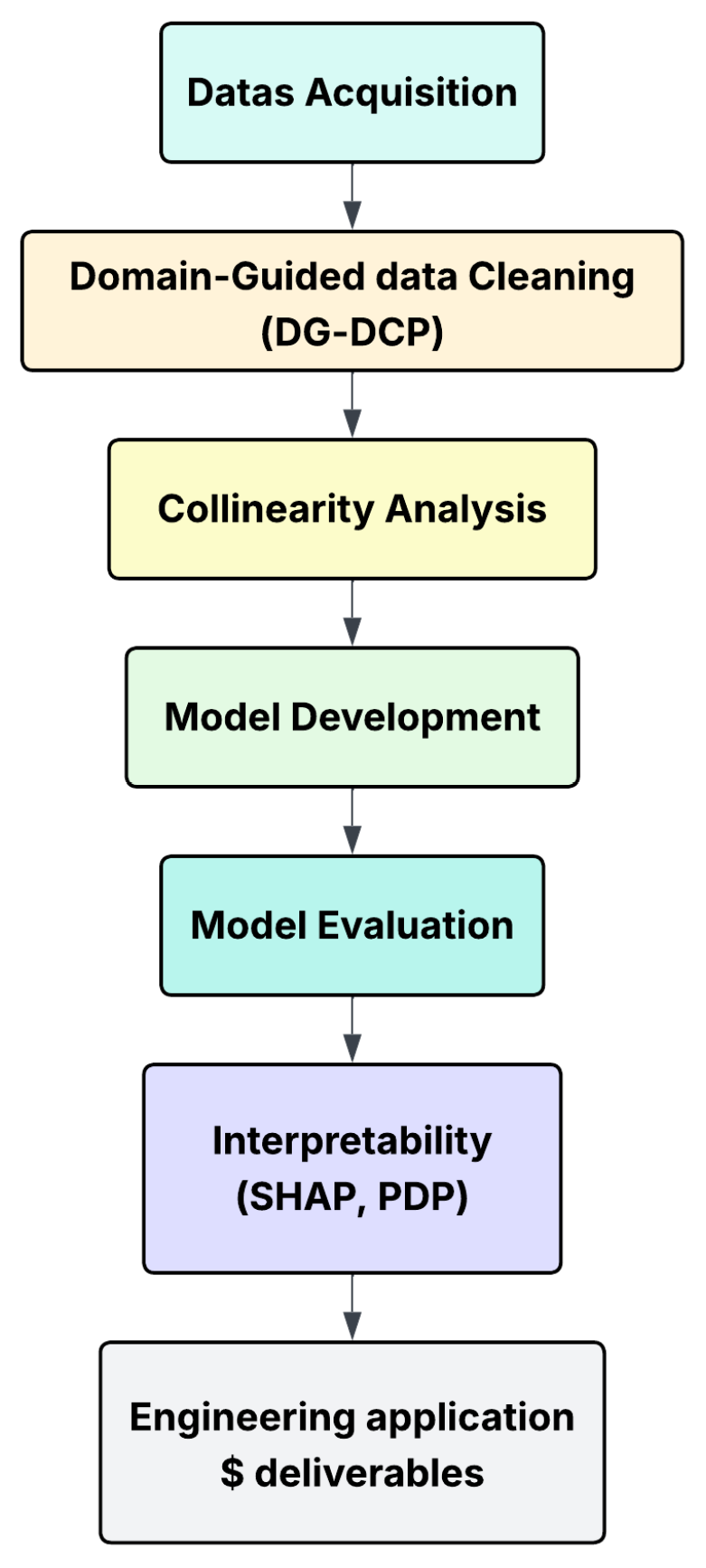
SP	Swell potential	Swelling on wetting	%	Lab test

. The five input predictors are (LL%), plastic limit (PL%), plasticity index (PI%), Skempton activity (A = PI/C), and clay fraction (C%). The model’s output label is swell potential (SP%). The complete research workflow, from raw data acquisition to engineering deliverables, is summarized schematically in Figure 1.

Missing-value imputation was deliberately avoided to preserve geotechnical fidelity. Although fewer than 27% of rows contained missing values, the omissions were confined to laboratory-derived variables rather than random errors. Inputting such quantities using statistical methods (e.g., k-nearest neighbors or MICE) would create synthetic laboratory results, violating fundamental principles of soil mechanics. For example, assigning a liquid limit of 60% to a kaolinitic sample could mimic montmorillonitic behavior and severely distort swell predictions. In addition, the missingness exhibited a clear structure, typically affecting variables that require specialized testing, which invalidates the “missing at random” (MAR) assumption central to most imputation techniques [62,63]. Where missing values could be deterministically reconstructed (e.g., PI = LL − PL, or A = PI/C), they were back-calculated. Specifically, 109 missing values for activity (A) and 19 for clay content (C) were successfully recovered using these deterministic relationships. Records that could not be reconstructed were excluded from the analysis. This approach avoided synthetic noise, ensured physical validity, and preserved methodological control between the raw and cleaned datasets.

Descriptive statistics for the Model 1 dataset are summarized in

Table 2. Descriptive statistics dataset used in Model 1.

Statistic	SP	LL	PL	PI	A	C
Mean	22.49	69.32	26.25	43.07	2.44	44.07
Std. Dev.	23.52	27.17	6.59	25.68	9.61	16.24
Min	0.26	19	4	7.1	0.24	2.5
25%	8.50	54	21	26.2	0.64	30
Median	15.55	68.5	26	40	0.85	50
75%	25.63	78	28	54	1.03	53.34
Max	168.57	255	66	225	90	93
Skewness	2.68	2.37	1.26	2.89	6.95	−0.15

. Swell potential (SP) spans a wide range, from 0.26% to 168.57%, with a standard deviation of 23.52% and strong right skew (2.68), reflecting the presence of high-swell cases and distributional imbalance. Liquid limit (LL) ranges from 19% to 255%, and plasticity index (PI) reaches an implausible maximum of 225%, indicating likely data-entry errors and confirming PI’s deterministic dependence on LL and PL. Activity (A), computed as PI divided by clay content, shows the highest variability, with a standard deviation of 9.61 and extreme right skew (6.95). Most notably, A reaches a maximum value of 90, which far exceeds the range associated with any natural clay mineral. For reference, even highly active montmorillonitic clays typically exhibit A values between 5.6 and 13.9 [64]. Such an outlier is physically implausible and suggests a unit mismatch or transcription error. This further motivates the need for domain-guided data cleaning.

3.1. Baseline Model

The baseline configuration (Model 1) represents an “as-received” treatment, commonly adopted in early-stage applications of ML to geotechnical datasets. This model utilizes the original, unprocessed file, comprising 310 observations, each characterized by five numerical predictors: liquid limit (LL %), plastic limit (PL %), plasticity index (PI %), Skempton activity (A = PI/C), and clay fraction (C %), with swell potential (SP %) as the response variable. No preprocessing steps were applied to this dataset. Specifically, no hard-limit filtering, categorical validation, or duplicate removal procedures were performed, and fundamental deterministic relationships, such as PI = LL − PL, were not enforced. As a result, potential transcription errors (e.g., PI > LL), statistical outliers, and duplicate records remain within the modeling matrix. Diagnostic inspection revealed that the dataset contains several exact duplicate rows as well as extreme values in key geotechnical indices, most notably abnormally high PI, LL, and A values, suggesting either entry errors or the absence of threshold-based screening. Moreover, full multicollinearity among LL, PL, PI, and A is preserved, and no effort was made to identify or mitigate redundant predictors.

Model 1 is deliberately structured to expose the methodological risks associated with disregarding geotechnical domain knowledge and statistical best practices. These risks include artificially inflated variance-explanation statistics, elevated sensitivity to extreme residuals, and impaired model interpretability due to overlapping and collinear features. The evaluation metrics derived from this configuration thus serve as a benchmark against which the performance of the domain-informed, multicollinearity-aware alternative is later assessed.

3.2. Domain-Guided Cleaning Pipeline (DG-DCP)

The cleaning process incorporated a series of domain-specific rules designed to enforce geotechnical plausibility, consistency with classification systems, and basic physical realism. These checks were applied sequentially, and rows were either flagged for review or removed outright, depending on the severity and nature of the violation.

Initial hard limits were imposed to discard values falling outside physically meaningful ranges, such as negative Atterberg indices or swell potential, or clay contents exceeding 100%. Beyond these bounds, plausibility bands were defined to identify extreme but potentially valid entries such as LL > 200%, PI > 70%, or A > 10 that warrant manual review rather than automatic exclusion. To ensure internal numerical consistency, computed activity values (PI divided by clay fraction) were compared to reported ones, and rows with discrepancies beyond a small tolerance were flagged. Cases where swell potential exceeded 40% while plasticity index remained below 10% were also considered anomalous, as they suggest an unrealistic decoupling of plasticity from swelling behavior.

Further validation was carried out by comparing each sample’s position on the Casagrande plasticity chart with the expectations implied by its USCS code [65]. Soils classified as coarse-grained (e.g., GW, GP, SW, SP) were expected to exhibit clay contents below 5%, while fine-grained groups (e.g., ML, CL, MH, CH) were expected to exceed 15% clay. Any mismatch between textural classification and clay content was flagged as a potential indication of mislabeling or sampling inconsistency. The complete set of applied conditions is summarized in

Table 3. Geotechnical validation checks.

Check Description	Condition
Hard limits	Drop if: LL < 0, PL < 0, PI < 0, SP < 0, Clay > 100
Plausibility band	Flag if: LL > 200, PI > 70, PL > 80, A > 10, SP > 100
Activity consistency	Flag if: |A − (PI/(Clay/100))| > 0.2
Swell–plasticity inconsistency	Flag if: SP > 40 and PI < 10
Casagrande vs. USCS check	(LL, PI) point must fall in USCS-implied zone
USCS–clay content sanity	GW, GP, SW, SP → Clay < 5
USCS–clay content sanity	ML, CL, MH, CH → Clay > 15

. The combined application of these rules ensured that the dataset used for modeling conformed to geotechnical reasoning and empirical expectations while still preserving edge cases for manual review when needed.

3.3. Collinearity and Feature Selection

Before finalizing the predictive model, a collinearity assessment was performed to ensure that the selected input features supported both statistical reliability and geotechnical interpretability. Although ensemble models, such as random forests, are generally robust to collinearity in terms of prediction accuracy, the presence of redundant or highly correlated predictors can distort feature importance rankings and obscure the underlying physical relationships that the model is meant to capture. Therefore, feature selection in this study was guided not only by predictive performance but also by collinearity structure and geotechnical reasoning.

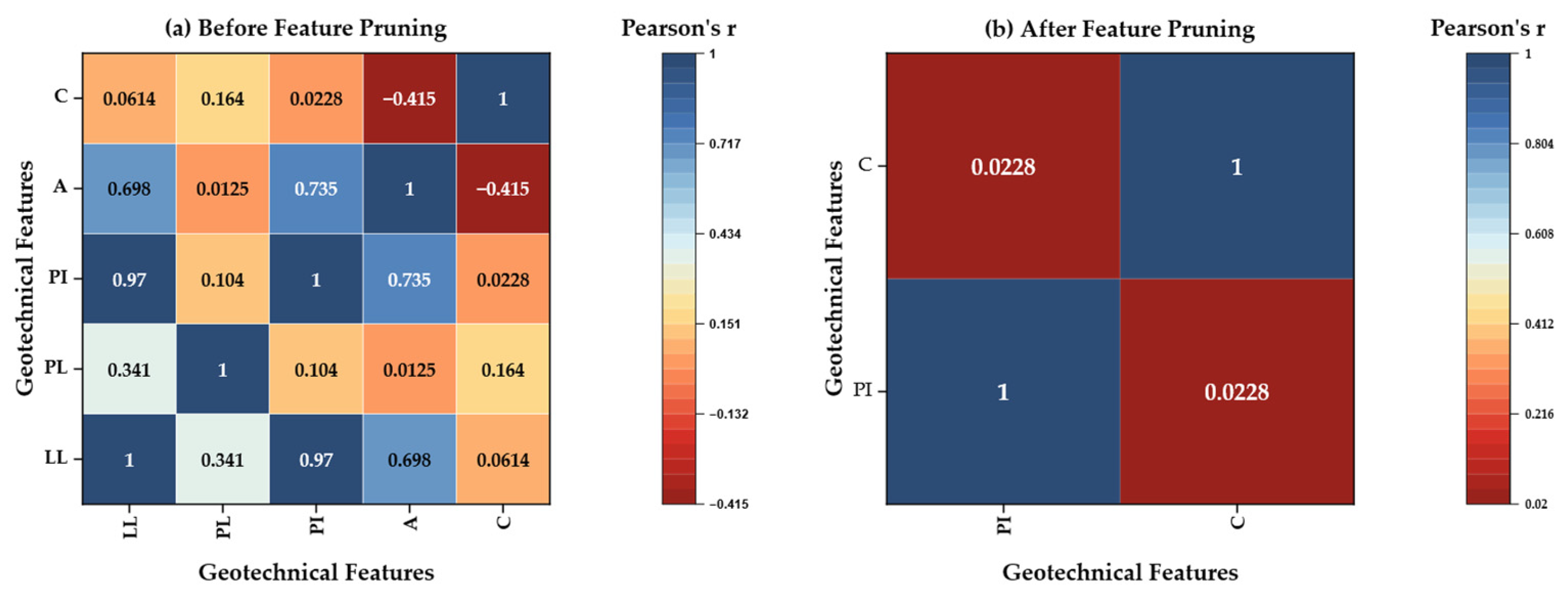
Figure 2 illustrates, in two side-by-side heat-map panels, how domain-guided feature pruning transforms a highly collinear five-variable space into an orthogonal two-variable set. In panel (a), “Before Feature Pruning,” the 5 × 5 matrix depicts Pearson correlation coefficients among liquid limit (LL), plastic limit (PL), plasticity index (PI), Skempton activity (A = PI/C), and clay fraction (C). The color scale, ranging from deep blue (r = +1) through white (r ≈ 0) to deep red (r = −0.42), highlights very strong collinearity between LL and PI (r = 0.97) as well as moderate association of LL with activity (r = 0.698) and negligible association with clay fraction (r = 0.061). The single red cell (activity versus C, r = −0.415) reflects the mathematical definition of activity. At the same time, all other off-diagonal correlations remain small (|r| ≤ 0.17), indicating minimal shared variance among the remaining variable pairs.

In panel (b), “After Feature Pruning,” LL, PL, and activity have been removed, leaving only PI and clay fraction. The resulting 2 × 2 matrix, plotted with the same color scale, exhibits an off-diagonal correlation of r = 0.0228, which is effectively zero and is rendered as a neutral hue. The disappearance of saturated blues underscores the successful elimination of redundant information. Together, the two panels confirm (1) the exact linear dependence among LL, PL, and PI; (2) the derived nature of activity, and (3) the statistical independence of the retained predictors, PI and C, conditions that underpin the stability and interpretability of the final random forest model.

Table 4. Variance-inflation factors (VIF) before and after feature pruning.

Predictor	Before	After
	5 Features	2 Features
LL	∞	-
PL	∞	-
PI	∞	1.00
A	3.65	-
C	1.71	1.00

presents the corresponding variance inflation factors: LL%, PL%, and PI%. All three return infinite values due to exact linear dependence (PI = LL − PL), while activity records a VIF of 3.65, indicating problematic redundancy. Only the clay fraction maintains an acceptable VIF of 1.71. On statistical grounds, LL, PL, and activity were therefore excluded from the final feature set.

The rationale for this exclusion is supported by domain logic. The plasticity index already encapsulates the essential difference between LL and PL and is widely recognized in geotechnical engineering as a primary indicator of swell potential. Similarly, activity is derived by normalizing PI concerning the clay fraction, making it mathematically dependent on the retained variables. By keeping PI (representing the quality of expansive minerals) and clay content (representing their quantity), the model preserves two orthogonal drivers of swelling behavior while avoiding multicollinearity. The refined feature set exhibits a near-zero Pearson correlation (r = 0.02) and VIF values of 1.00 for both predictors, confirming statistical independence.

3.4. Model Training and Evaluation

Using the raw dataset described in Section 3.2 (310 records; five index properties), we trained Model 1 as follows: because high-swell cases are sparse, SP values were binned into quintiles, and an 80:20 stratified shuffle split (seed = 42) was created so that each subset preserved the same proportion of low-, medium-, and high-swell samples found in the complete raw dataset. This approach was further justified by the strong right skew observed in SP (skewness = 2.68), which indicated a concentration of samples in the low-swell range and a long tail of high-swell outliers. Stratified binning ensured balanced representation of all ranges across both the training and test sets, thereby improving the robustness of performance evaluation. This split served as the primary hold-out strategy, providing a fixed test set against which all model predictions were evaluated.

Random forests were selected for their strong alignment with the geotechnical, statistical, and interpretability needs of this study. Swell potential involves non-linear, threshold-driven behavior, such as rapid increases beyond PI ≈ 50%, which tree-based models capture naturally without assuming specific functional forms or requiring kernel tuning [18]. Given the modest dataset size (n = 310–291), random forests offer better stability than GBMs or neural networks, which often overfit in small-sample contexts [66]. They also require minimal preprocessing, preserving the physical meaning of geotechnical indices without normalization. Their interpretability is a further strength: split frequencies yield intuitive feature rankings, TreeSHAP produces auditable attributions, and known relationships, such as that between PI and swell, are transparently reflected [18]. Finally, forests enable empirical prediction intervals via tree variance, supporting bootstrap-based uncertainty estimation without distributional assumptions [67,68].

A random-forest regressor (200 trees, unlimited depth, random_state = 42) was trained for each dataset. Hyperparameter tuning was deliberately omitted to isolate the impact of data-quality interventions. Model accuracy on a fixed 20% hold-out set was summarized using R², MAE, RMSE, and the most significant residual. Generalization and uncertainty were quantified with a 10 × 3 stratified cross-validation and a 1000-rep bootstrap (complete metric definitions in Table S1, Supplementary Information).

Model 2, which retains 291 rows after hard-limit filtering, USCS [65] validation, and duplicate removal. Multicollinearity diagnostics leave only two predictors, PI% and clay fraction C%, in the matrix X₃. Because the row count changed, a fresh 80–20 stratified shuffle split was drawn, but the same quintile-based rule and the same random seed of 42 were used, resulting in a partition whose class proportions mirror those within the reduced dataset. This again served as the fixed hold-out test set for evaluating all downstream metrics. The identical random-forest hyperparameters were applied. The entire evaluation pipeline, single-split metrics and plots, repeated stratified cross-validation, 1000-rep bootstrap, and prediction-interval tally, was repeated without alteration. A comparison of the modeling configurations and training pipelines is summarized in

Table 5. Modeling workflow summary for Model 1 and Model 2.

Aspect	Model 1	Model 2
Dataset size	310 records	291 records
Cleaning steps	None	Geotechnical validation
Predictors (x)	LL, PL, PI, A, C	PI, C
Target (y)	Swell potential (SP)	Swell potential (SP)
Stratified split	80:20 (SP quintiles)	80:20 (SP quintiles)
Random seed	42	42
Model type	Random forest regressor	Random forest regressor
Hyper-parameters	200 trees, unrestricted depth	200 trees, unrestricted depth
Hold-out test	Yes	Yes
Cross-validation	10 × 3 StratifiedKFold	10 × 3 StratifiedKFold
Bootstrapping	1000 reps, fixed test	1000 reps, fixed test
Diagnostic plots	Residual and fitted plots	Residual and fitted plots
Interpretability tools	SHAP plots, PDPs	SHAP plots, PDPs

.

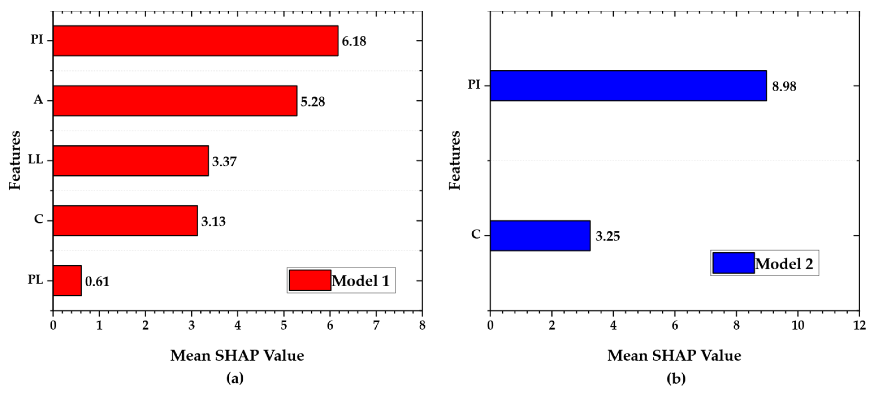
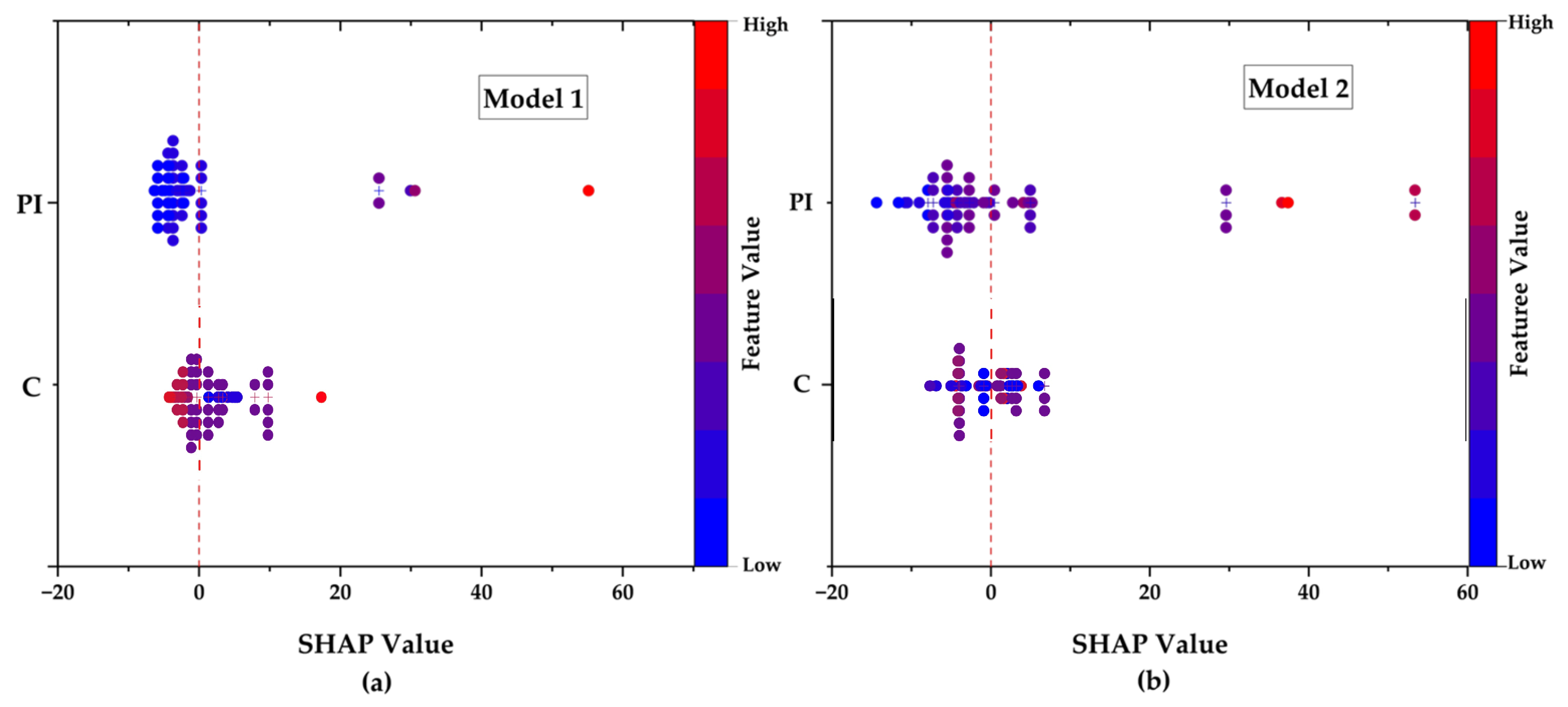
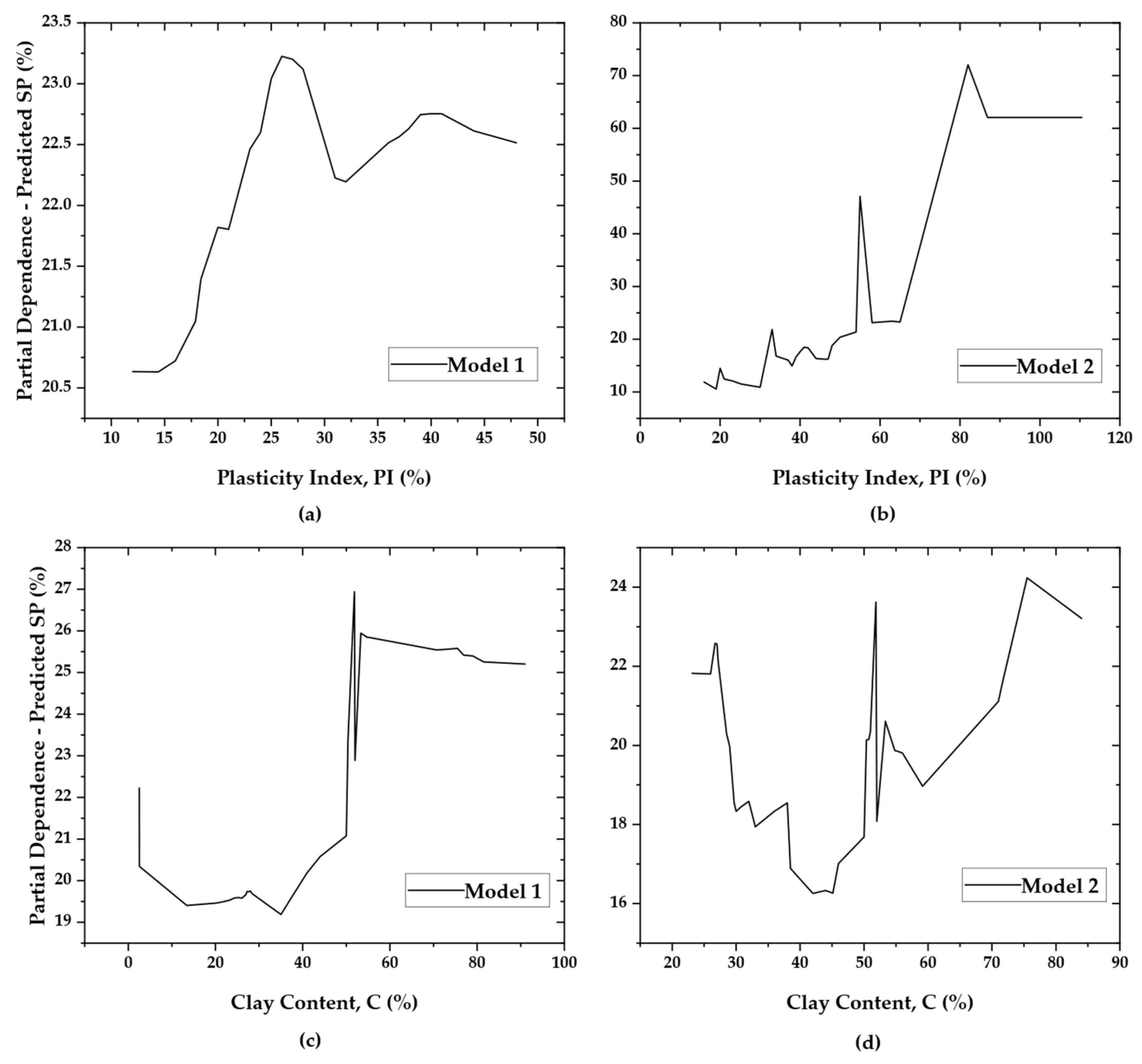
For interpretability, TreeSHAP values were calculated on the hold-out set, and a mean |SHAP| bar chart and a beeswarm plot were generated. Partial dependence curves for PI% and C% provided a clear view of the marginal responses. By maintaining the same stratification logic, resampling schedule, bootstrap procedure, and model hyperparameters while only varying the data-quality interventions, this design isolates the impact of systematic cleaning and multicollinearity-aware feature pruning on predictive accuracy, error robustness, and geotechnical interpretability.

4. Results

4.1. Dataset Refinement via DG-DCP

The DG-DCP, as described in Section 3.3, was applied to the original dataset of 310 records to ensure geotechnical plausibility and internal consistency. As a result, 19 records (representing 6.1 percent of the dataset) were excluded, yielding a refined dataset of 291 entries suitable for subsequent modeling.

Nine of the excluded records exhibited extremely high Skempton activity values, calculated as the ratio of plasticity index (PI) to clay content (C). Reported values ranged from approximately 20 to 90, even though activity in natural soils generally does not exceed 4 [69]. Even highly active montmorillonitic clays rarely surpass 2.5 [70], and the highest documented values in the literature approach 13.9 [71]. Moreover, these samples had exceptionally low clay contents, approximately 2.5 percent, rendering such high activity values physically implausible. These anomalies strongly suggest transcription errors, improper unit scaling, or data entry issues and were therefore removed.

Seven additional records were identified as exact duplicates, identical across all recorded variables. These corresponded to a specimen with a PI of 38 percent, a clay content of 52 percent, and a swell potential of between 12 and 14 percent. In the context of geotechnical laboratory testing, it is highly improbable for multiple independent samples to produce perfectly matching values due to the inherent heterogeneity of soils and measurement variability [72]. Retaining these duplicates would have disproportionately weighted a single test result, potentially distorting model training and residual analysis. Consequently, they were excluded.

The remaining three records were removed due to internal inconsistencies between index properties and textural composition. Although their Atterberg limits placed them within the fine-grained region of the Casagrande plasticity chart (e.g., PI between 9% and 18%; LL between 21% and 33%), their reported clay contents were all below 15%. This violates expectations under the USCS [65], which requires coherence between plastic behavior and fines content [65]. Furthermore, these samples presented additional red flags. Each of these samples exhibited unusually high swell potential (17–19%), despite having low plasticity index (PI) and liquid limit (LL) values, as well as activity ratios (A = PI/clay fraction) below 1.3. Such a combination contradicts well-established geotechnical understanding, where expansive behavior is typically associated with high plasticity, significant clay content, and moderate to high activity values. These mismatches between swell behavior, plasticity, and clay fraction suggest data inconsistencies that could not be reconciled through mineralogical or procedural explanations [73]. As such, they were deemed unreliable and removed under the DG-DCP.

The elimination of these 19 anomalous records effectively truncated the extreme tails of key variables while preserving the integrity of their central distributions. Maximum PI decreased from 225 percent to 110.5 percent, and maximum swell potential declined from 168.6 percent to 92.8 percent. The means and medians of PI, clay content, and swell potential remained broadly stable. Additionally, skewness for swell potential declined from 2.68 to 1.89, and for PI from 2.89 to 0.53, as summarized in

Table 6. Summary statistics before and after DG-DCP.

Feature	Metric	Model 1 (n = 310)	Model 2 (n = 291)
SP (%)	Mean	22.49	20.45
	Std. Dev.	23.52	18.19
	Min–Max	0.26–168.57	0.26–92.78
	Skewness	2.68	1.89
PI (%)	Mean	43.07	40.64
	Std. Dev.	25.68	18.15
	Min–Max	7.10–225.00	7.10–110.50
	Skewness	2.89	0.53
C (%)	Mean	44.07	45.56
	Std. Dev.	16.24	14.63
	Min–Max	2.50–93.00	17.00–93.00
	Skewness	−0.15	0.28

. The resulting dataset retains the intrinsic variability of expansive soils while excluding physically implausible values, redundant observations, and classification conflicts, thereby providing a robust and defensible foundation for model development and interpretability analysis.

4.2. Comparative Model Performance

Quantitative outcomes for both experiments are summarized in

Table 7. Performance comparison of Model 1 and Model 2 across all evaluation schemes.

Metric	Model 1 (5 Predictors)	Model 2 (2 Predictors)	∆ % †
Single hold-out split
R2	0.8628	0.8432	−2.3
MAE (%)	5.95	5.352	−10.0
RMSE (%)	8.967	6.784	−24.3
Worst residual (%)	41.87	15.88	−62.0
10 × 3 stratified CV (mean ± SD)
R2	0.815 ± 0.105	0.741 ± 0.186	−9.1
MAE (%)	6.337 ± 1.264	6.032 ± 1.046	−4.8
RMSE (%)	9.029 ± 2.716	8.390 ± 2.095	−7.1
1000-rep bootstrap
Median RMSE (%)	10.066	7.497	−25.5
95% RMSE CI (%)	7.836–13.158	6.556–10.085	-
95% PI coverage (%)	51.8	54.3	+2.5 pp

^† Percentage difference: (Model 1 − Model 2)/Model 1 × 100.

and visualized in Figure 3.

On the fixed 20% hold-out set, Model 2 (domain-cleaned, two inputs) lowered RMSE from 8.97% to 6.78% (−24%) and cut the worst residual from 41.9% to 15.9% (−62%) relative to Model 1 (Table 7). That sharp reduction in the error tail is critical for reliability-based design, where extreme under-predictions control safety margins.

In 10 × 3 stratified cross-validation, RMSE fell from 9.03% ± 2.72% to 8.39% ± 2.10%, while bootstrap analysis (1000 reps) showed median RMSE dropping from 10.07% to 7.50% and a narrower 95% interval (6.56–10.09%). Prediction-interval coverage improved slightly to 54%. Overall, the domain-guided, two-feature model trades a slight decrease in R² for markedly tighter and safer error bounds.

To ensure that these performance gains generalize beyond a single split, three complementary validation schemes were employed. First, the 80:20 stratified hold-out test preserved the skewed SP distribution and provided a fixed reference for direct comparison. Second, a 10 × 3 stratified cross-validation, repeated over different folds, quantified both mean performance and its variability across random partitions, revealing the model’s stability under data shifts. Third, a 1000-rep bootstrap of the entire pipeline produced empirical confidence intervals for RMSE and achieved 95% coverage, thereby capturing sampling uncertainty and the model’s error distribution tail. Together, these schemes confirm that the domain-pruned model’s improvements in RMSE and extreme-residual reduction are robust, reliable, and not artifacts of a single random split. As visualized in Figure 3, the blue bars representing Model 2 are uniformly shorter than the blue bars for Model 1 across all error metrics, confirming the trends reported in Table 7.

4.3. Residual Diagnostics

Figure 4 and Figure 5 convey complementary diagnostic information on model behavior after the domain-guided cleaning procedure. Figure 4 plots the signed residuals (observed-predicted swell potential) against the model’s predictions. This residual-versus-prediction view is designed to reveal heteroscedasticity and scale-dependent bias. Model 1 (Figure 4a) exhibits a pronounced funnel, with error variance increasing steadily and individual underpredictions reaching −42% at the highest swell levels. By contrast, Model 2 (Figure 4b) collapses the funnel; 96% of residuals fall within ±15%, and the largest error is limited to −16%. The horizontal axis here is the predicted value, so any curvature or spreading pattern directly signals where the model loses stability as the magnitude of the estimate grows.

Figure 5 is an observed-versus-predicted plot. Both axes carry the swell value itself, and the red 1:1 line represents perfect calibration. Departures from this diagonal highlight systematic over- or under-estimation across the entire response range rather than variance at a given scale. Model 1 (Figure 5a) overshoots virtually every specimen above 60% swell, confirming the bias hinted at in Figure 4. Model 2 (Figure 5b) tracks the diagonal from 0% to 90%, indicating that the two-variable specification not only reduces error magnitude but also restores global calibration.

Taken together, the figures serve different analytical purposes: Figure 4 diagnoses error dispersion and outlier leverage, whereas Figure 5 evaluates the absolute agreement between measurements and predictions. Demonstrating improvements in both views establishes that the domain-informed cleaning and feature pruning enhance the model’s reliability in terms of variance control and bias removal.

Table 8. Error quantiles (|residual|%) for Model 1 vs. Model 2.

Quantile	Model 1	Model 2
10%	0.54	0.19
25%	1.33	2.02
50% (median)	4.54	4.64
75%	8.47	8.29
90%	13.84	10.95
95%	16.13	12.97
99%	28.18	15.13

provides a more detailed examination of the error distribution. The median absolute error stays about the same (4.54% in Model 1 vs. 4.64% in Model 2). Still, the larger errors are significantly reduced: the 90th percentile error drops from 13.8% to 11.0%, the 95th percentile from 16.1% to 13.0%, and the 99th percentile is cut in half, from 28.2% to 15.1%. This significant reduction in extreme errors lowers the risk of serious underpredictions in engineering design [72]. There is a slight increase in the 25th-percentile error (from 1.33% to 2.02%), which suggests that some of the low-error sharpness in the raw model resulted from overfitting simple cases, a phenomenon that model 2 avoids by removing unnecessary predictors [74]. Overall, these diagnostics confirm that Model 2 maintains the same overall accuracy while significantly reducing high-impact errors.

4.4. Interpretability via SHAP and PDP

To assess the internal reasoning of the random forest models and ensure consistency with established soil behavior, interpretability analyses were conducted using SHAP and PDPs. These methods quantify the contribution of individual features to predicted outcomes, enabling a transparent evaluation of how the model learns geotechnically relevant patterns.

Figure 6 presents the SHAP feature importance summary for both models. In Model 1, where five predictors were used, feature attributions are diffused across several highly collinear variables: PI, LL, and activity, each receiving substantial weight. This redundancy reflects the underlying multicollinearity in the raw dataset, where PI is mathematically dependent on LL and PL, and activity is derived from PI and clay content. Such overlap complicates interpretation and risks overstating the influence of a single geotechnical property across multiple redundant representations [75]. In contrast, Model 2 presents a cleaner attribution structure. PI accounts for approximately 75% of the explanatory power, and clay content (C) contributes the remaining 25%. This split aligns well with domain knowledge, where PI reflects the mineralogical reactivity of the soil [70], and clay content demonstrates the abundance of expansive materials [64].

Figure 7 presents a comparative analysis of the SHAP beeswarm summaries for the full five-variable random forest (Model 1) and its reduced two-variable counterpart (Model 2). In each plot, the horizontal axis reports the SHAP contribution in percent swell potential, with samples to the right of the vertical zero line exerting a positive uplift on the predicted swell relative to the global mean. In contrast, those to the left have a suppressive effect, and the color gradient from deep blue to deep red encodes the raw feature magnitude. By plotting every hold-out specimen, these beeswarm diagrams simultaneously reveal both the directionality and magnitude of each predictor’s influence across the entire dataset.

In Figure 7a, Model 1’s plasticity-index subplot shows that, while specimens with PI below 30 percent remain clustered near zero, higher-PI observations scatter indiscriminately on both sides of the zero line. This dispersion suggests that the model’s interpretation of PI is confounded by its correlation with three additional predictors, resulting in inconsistent SHAP values for high-plasticity soils. Likewise, the clay-fraction subplot for Model 1 displays numerous high-clay samples registering negative SHAP contributions. This result contradicts the well-established geotechnical principle that increasing clay content tends to augment swell potential. These erratic patterns arise because multicollinearity among the five features forces SHAP to partition influence arbitrarily among redundant predictors, thereby obscuring the actual physical effect of each variable.

By contrast, Figure 7b demonstrates that Model 2, retaining only plasticity index and clay fraction after domain-guided feature pruning, restores clear, monotonic relationships aligned with soil mechanics theory. In the PI plot, low-plasticity specimens consistently yield negative SHAP values, while high-plasticity specimens shift uniformly toward positive contributions, resulting in a coherent left-to-right gradient of blue through red points. The clay-fraction subplot exhibits a similarly smooth progression of SHAP contributions with increasing clay content, mirroring the classical saturation behavior of expansive minerals. Eliminating the redundant collinear predictors not only sharpens the individual SHAP distributions but also enhances interpretability, confirming that the two-variable model delivers a more parsimonious and geotechnically plausible depiction of how soil index properties govern swell potential.

Figure 8a,b compares the partial dependence of the plasticity index (PI) for the complete five-variable model (Model 1) and the reduced two-variable model (Model 2). In Figure 8a, the PI curve for Model 1 rises from about 20.6% at PI ≈ 15% to a local maximum of 23.2% at PI ≈ 27%, then unexpectedly declines to 22.2% by PI ≈ 33% before climbing again and flattening. This nonmonotonic behavior, with multiple inflection points, lacks a clear mechanistic rationale and reflects the confounding influence of redundant predictors. By contrast, Figure 8b shows that Model 2 remains essentially invariant for PI below 45% and then exhibits a marked threshold-type increase, with swell potential accelerating sharply beyond this critical plasticity level. Such a threshold response aligns with classic empirical swell charts and reinforces the central role of PI once extraneous variables are removed.

Figure 8c,d presents the analogous comparison for the clay fraction (C). The Model 1 curve in Figure 8c displays erratic kinks and abrupt jumps that do not correspond to any known mineral-saturation process but rather to competing signals from collinear features. In Figure 8d, the Model 2 curve follows a smooth, concave-up trajectory: predicted swell potential declines slightly through intermediate clay contents and then rises steadily at high clay fraction, reflecting progressive saturation of expansive minerals. It should be noted that clay fraction alone is not determinative of swelling unless the clay mineralogy includes expansive phases; soils dominated by non-expansive minerals such as kaolinite or illite may exhibit lower swell even at high clay content. By pruning out redundant predictors, the two-variable model restores a geotechnically plausible and interpretable relationship between clay content and swell potential.

Together, these interpretability results confirm that Model 2’s simplified predictor set, refined through domain-guided cleaning and collinearity pruning, retains both predictive power and mechanistic transparency. The feature attributions align with physical expectations, respond appropriately to key thresholds, and differentiate between mineralogically distinct soil types. For practical geotechnical applications, where model trust and explainability are essential, such behavior significantly enhances the model’s credibility and usability [76].

5. Discussion

5.1. Effect of Data Cleaning

The application of the DG-DCP resulted in meaningful structural improvements in both the dataset and model behavior, surpassing what traditional preprocessing or statistical cleaning methods could offer [58]. This cleaning process involved the removal of duplicate records, geotechnically implausible values (e.g., extreme activity ratios), and multicollinear features derived from deterministic relationships (e.g., PI vs. LL and PL) [74]. These steps were not merely statistical conveniences; they were informed by domain knowledge and rooted in the physical constraints of expansive soil behavior. As such, the effect of DG-DCP can be understood along three axes: data integrity, predictive reliability, and interpretability.

From a data perspective, the removal of just 19 problematic records (6.1%) resulted in a substantial improvement in dataset quality. Key variables such as PI and SP saw their extreme outliers removed (PI max reduced from 225% to 110.5%, SP from 168.6% to 92.8%), and their skewness values declined by more than 30%, resulting in a more statistically and geotechnically balanced dataset. Importantly, the central tendencies of these features were preserved, suggesting that DG-DCP eliminated anomalies without distorting the overall distribution of soil behaviors. This preservation of structural validity is essential when modeling nonlinear targets, such as swell potential, which are sensitive to both the presence and balance of high-variance cases [18].

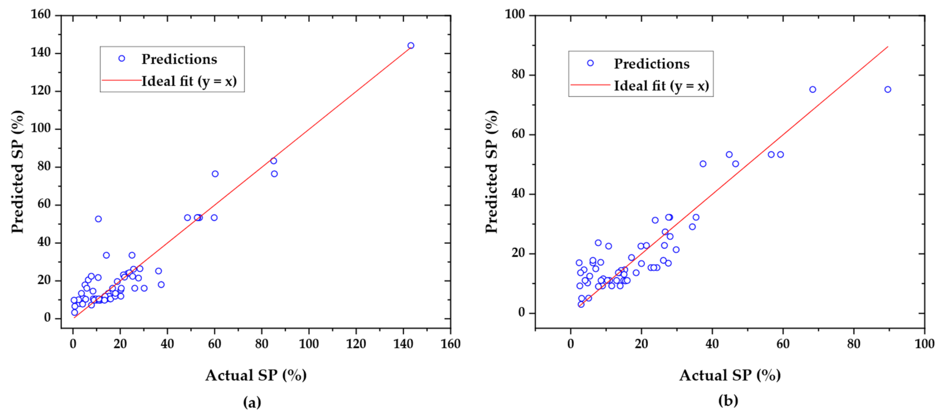
Model 1’s residuals displayed a pronounced funneling effect; errors increased in magnitude as predicted SP increased, and several points exceeded −40%. Model 2 eliminated this funnel shape. In this model, 96 percent of residuals fell within ±15 percent, with the worst error only −16%. Quantile-based error analysis revealed that Model 2 substantially reduced high-end error percentiles. For example, the 99th percentile decreased from 28.2% to 15.1%, and the 95th percentile declined from 16.1% to 13.0%, while the median performance remained nearly unchanged. Although the 25th percentile error slightly increased, this likely reflects the reduction of mild overfitting in Model 1, where redundant predictors may have artificially sharpened predictions on simpler samples. In short, DG-DCP replaced marginal overfitting with consistent reliability across the entire prediction range [74,77].

Finally, model interpretability saw a marked improvement. In Model 1, SHAP analysis revealed diffuse feature attributions across PI, LL, and activity, all of which were highly correlated. This redundancy complicated causal reasoning, as influence was spread across mathematically dependent features. In contrast, Model 2’s SHAP summary attributed 75% of predictive power to PI and the remaining 25% to clay content, aligning with known geotechnical principles [18,41]. The SHAP beeswarm plot revealed PI’s nonlinear and threshold-like behavior, particularly beyond 50%, consistent with expansive montmorillonitic clays [64,78]. Partial dependence plots revealed smooth, monotonic relationships between predictors and SP, indicating that the model’s behavior was not only accurate but also physically plausible [77]. In practice, this clarity is critical: geotechnical engineers require not only performance but also transparency, particularly when predictive models are to inform design or mitigation strategies [79].

5.2. Role of PI and Clay Content

As demonstrated by the SHAP and PDP analyses in Section 4.4, model behavior is driven almost exclusively by two orthogonal factors: the plasticity index (accounting for roughly 75% of the feature influence) and the clay fraction (about 25%). Once the plasticity index surpasses approximately 50–55%, it triggers a pronounced swell response, whereas the clay content contributes a steady yet saturating effect. This elegant two-variable partition encapsulates the classic quality-versus-quantity paradigm in expansive soils: the plasticity index gauges the reactivity of the clay minerals present. In contrast, the clay fraction quantifies the volume of that reactive material [18,80].

From a design standpoint, this distinction allows engineers to triage sites swiftly. A soil sample with 60% clay but a plasticity index of 20% (typical of kaolinite) poses minimal risk. In contrast, one exhibiting only 35% clay yet a plasticity index of 70% (indicative of montmorillonite dominance) warrants immediate mitigation, even though its clay content is lower. Consequently, routine plasticity index determinations and hydrometer tests provide sufficient insight for an initial go/no-go decision, obviating the need for costly oedometer swell tests on clearly benign samples.

Moreover, the two-variable model integrates seamlessly into digital workflows. Because plasticity index and clay fraction are routinely recorded in borehole databases, the model can be embedded directly into GIS layers, BIM plug-ins, or mobile field applications with virtually no additional data overhead. Users then obtain an interpretable risk index complete with bootstrap-derived uncertainty bounds without wrestling with collinear indices or specialized mineralogical inputs, enabling faster, more defensible decisions in foundation design and site zoning.

5.3. Engineering Applications

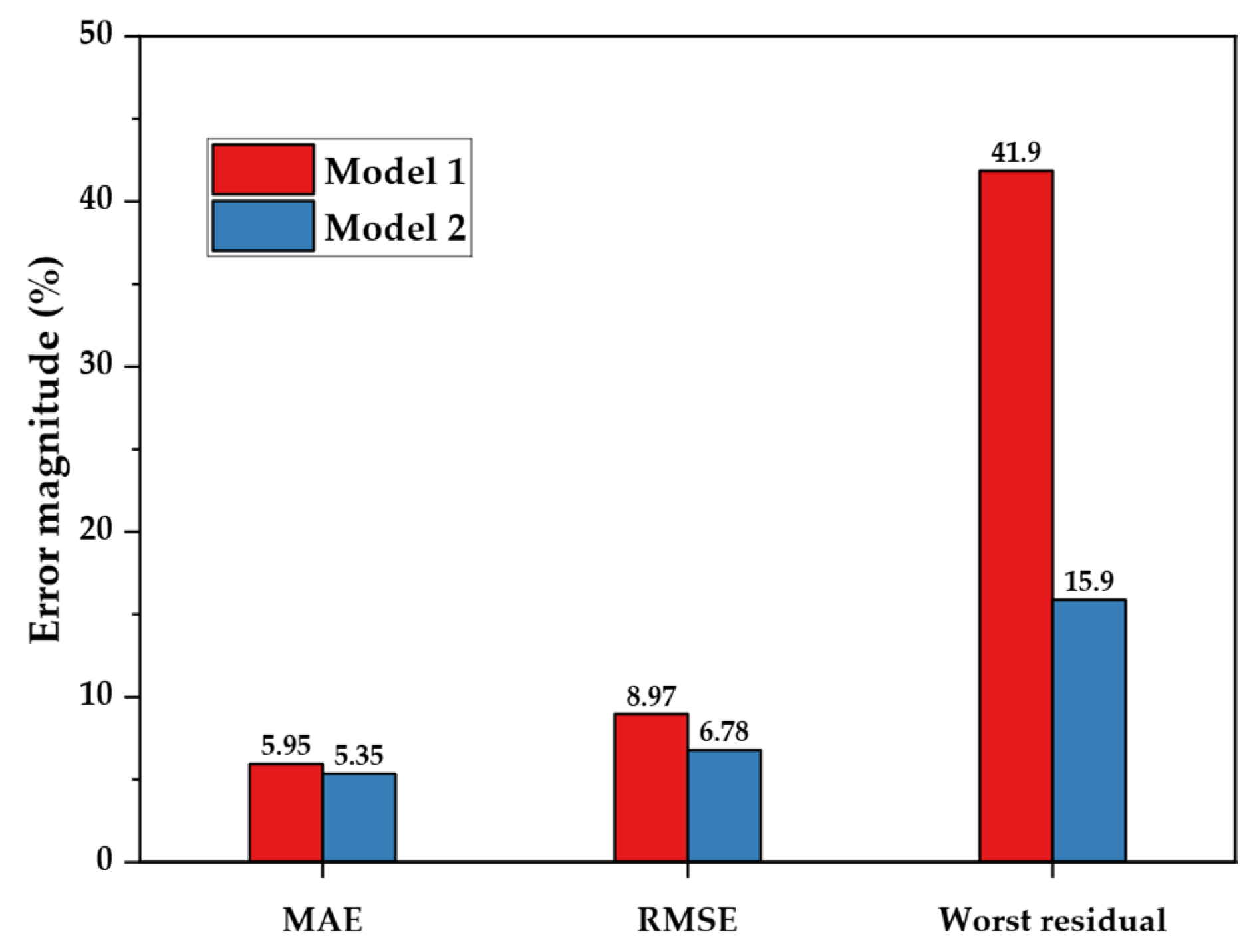
For building engineers, a swell-prediction model is valuable only if it improves judgment and lowers risk on real projects. The domain-guided Model 2 meets that test. By cutting the worst-case error from 41.9% to 15.9%, it significantly reduces the chance of underestimating heave, which can crack slabs, tilt walls, or distress pavements. Because the model requires only plasticity index and clay fraction, two indices already recorded in routine USCS [65] or American Association of State Highway and Transportation Officials (AASHTO) investigations, it integrates easily into existing workflows. This includes low-budget sites where oedometer or X-ray tests are impractical. Practitioners can use its outputs to prioritize mitigation strategies such as lime treatment and moisture control, determine whether further testing is needed, or flag high-risk borings for design review.

Interpretability further boosts adoption. Partial-dependence and SHAP plots reveal a clear warning threshold at PI ≈ 55%, echoing classical empirical charts; this transparency enables engineers to communicate risk to clients and regulators without the “black-box” stigma. At larger scales, the two-input form is lightweight enough for GIS layers, BIM plug-ins, or mobile field apps, enabling the rapid mapping of swell hazard zones and the more intelligent allocation of lab budgets.

In sum, Model 2 combines accuracy, simplicity, and explainability, making it a practical tool for risk-aware foundation design and site classification in both urban and remote settings. Its success illustrates how domain-pruned machine-learning models can extend geotechnical judgment rather than replace it, paving the way for broader use of data-driven methods in building engineering.

Beyond the technical benefits, the two-variable model offers a clear cost advantage. A one-dimensional oedometer swell test (ASTM D4546 [60]) typically costs between USD 350 and USD 400 per specimen and requires up to one week for setup, loading, and moisture equilibration [81]. In contrast, the only laboratory inputs required were the Atterberg limits and a hydrometer-based determination of the clay fraction. These are routine classification tests that together cost approximately USD 120 per specimen and can be completed within 24–48 h [81]. Substituting the model for swell testing during preliminary site investigations therefore reduces direct laboratory expenditure by approximately 65–70% and delivers results several days earlier. For a moderate project (e.g., 20 boreholes × 3 samples = 60 specimens), this translates to a budget saving on the order of USD 16,000 while still flagging the minority of high-risk samples that warrant confirmatory swell tests. Used as a triage tool, the model thus complements, not replaces, conventional testing by focusing resources where they provide the most significant engineering value.

5.4. Limitations and Future Work

Although the two-variable model outperforms a fuller baseline, it nonetheless inherits several constraints. First, relying solely on plasticity index and clay fraction omits other physical drivers of swelling: mineralogical composition, soil suction, fabric, and moisture history. Their absence leaves appreciable unexplained variance and results in under-calibrated prediction intervals: empirical coverage reaches only 54% where 95% is desired. Second, the model’s generalization stability remains imperfect. The cross-validation R² dropped from 0.82 in the five-feature case to 0.74 after pruning, indicating sensitivity to shifts in local data distribution. Third, the cleaning pipeline, although necessary, reduced the working sample from 395 to 291 records, trimming many high-PI and high-swell observations and limiting geographic diversity. Moreover, the model’s transferability to regions with different clay mineralogies and climatic or geological conditions remains untested. Evaluating its performance across such diverse settings would be a valuable direction for future investigation.

Further research should therefore broaden both data and methods. Introducing causal variables, such as bentonite or kaolinite percentages obtained by X-ray diffraction, or suction and climate indicators, would capture mechanisms now missing and should tighten prediction intervals. Complementing random forests with quantile-based or conformal techniques offers a path to calibrated, site-specific uncertainty bounds. Adding spatial context (sampling depth, climate zone, moisture history) would, in turn, enable location-aware risk maps and BIM integrations. Finally, releasing the cleaned dataset, code, and interpretability notebooks via platforms like GitHub or Zenodo will promote external validation and adaptation to related geotechnical problems, pushing data-centric geomechanics toward models that are both statistically reliable and practically deployable in building-design workflows.

6. Conclusions

This study demonstrates that integrating geotechnical domain knowledge at the outset can produce more streamlined, reliable, and interpretable ML tools for expansive-soil design. Beginning with 395 laboratory swell records, a rule-based data cleaning pipeline was applied to eliminate implausible entries and exact duplicates, resulting in a refined dataset of 291 trustworthy cases. The DG-DCP removed nine samples with implausible activity values, seven exact duplicates, and three USCS-inconsistent records, yielding a geotechnically coherent dataset of 291 entries. Subsequent multicollinearity analysis reduced five overlapping index properties to the two most practically significant predictors: plasticity index (PI) and clay fraction (C).

A random forest trained on this pared-down dataset (Model 2) reduced the hold-out RMSE by 24% and lowered the worst residual from 42% to 16%, compared to a five-feature baseline model, despite a modest decrease in R². This slight R² reduction (from 0.863 to 0.843, a 2.3% decrease) reflects the removal of collinear predictors that contributed little unique variance. Its minimal magnitude has a negligible effect on explanatory power, especially given the model’s substantially tighter error bounds and improved reliability. SHAP and PDP diagnostics indicate that the swell risk increases sharply when the plasticity index (PI) exceeds approximately 55%, while the clay content (C) contributes a secondary, saturating influence. This behavior aligns closely with the known response of montmorillonitic clays. Since PI and C are routinely measured in standard site investigations, the model is readily deployable for early foundation screening, GIS-based hazard mapping, and integration into BIM plug-ins, particularly in contexts where oedometer testing is unavailable or cost-prohibitive.

Limitations remain. Missing mineralogical, suction, and fabric data cap predictive certainty, and tree-based prediction intervals still under-cover high-swell outliers. Future work should pair the same domain-guided philosophy with richer datasets, quantile or conformal forests, and external validation on new regions.

These findings underscore the value of geotechnically informed, parsimonious ML models in improving the reliability and transparency of swell potential forecasts. By leveraging only two routinely available inputs (plasticity index and clay fraction), this approach supports faster and more risk-aware decision making in the planning and structural design of low- to mid-rise buildings on expansive soils, particularly in regions where advanced testing is limited. Moreover, by replacing costly oedometer swell tests with routine Atterberg limit and clay fraction measurements, this two-variable model can reduce preliminary site investigation costs by roughly 65–70% while proactively flagging high-risk borings to prevent subsidence- and swell-related structural damage.