Fire Resistance of Steel Beams with Intumescent Coating Exposed to Fire Using ANSYS and Machine Learning

Abstract

The thermal conductivity of steel is high compared to other materials such as concrete or timber. Therefore, fire protection measures are applied to prolong the duration between the onset of fire exposure and the final loss of load-bearing function of a steel structure. The most common passive fire protection measure is the application of intumescent coating (IC), a thin film that expands at elevated temperatures and forms an insulating char layer of lower thermal conductivity. This paper focuses on structural steel beams with IPE open-section profiles protected by a water-based IC and subjected to static and standard fire loading. ANSYS 16.0 is used to simulate heat transfer, with thermal conductivity function described by standard multivariate linear regression analysis, followed by mechanical analysis considering degradation of material mechanical properties at elevated temperatures. Simulations are conducted for all IPE profile sizes, with varying initial degrees of utilisation, beam lengths, and coating thicknesses. Results indicated fire resistance times ranging from 24 to 53.5 min, demonstrating a relatively good level of fire resistance even with the minimal IC thickness. Furthermore, artificial neural networks were developed to predict the fire resistance time of steel members with IC using varying numbers of hidden neurons and subset ratios. The model achieved a predictability level of 99.9% upon evaluation.

1. Introduction

1.1. Fire Protection of Steel Members

Although building fires are perceived to have a low probability of occurrence, these events are incidents of high importance that may lead to tragic outcomes. For structures susceptible to fire, the most essential requirement is defined by their fire resistance time, meaning that structural fire resistance must be provided for a specified period of time. Steel’s high thermal conductivity compared to other structural materials such as concrete or timber causes rapid, uniform heat distribution, leading to progressive loss of load-bearing capacity. This is further highlighted for thin-walled steel members. To achieve the desired fire resistance, steel members are often protected using passive measures designed to provide shielding and insulation from direct fire exposure, while various performance-based fire protection methods are also being proposed [1]. The most common and architecturally preferred passive fire protection is the direct application of intumescent coating (IC) to the steel surface [2,3]. An IC is a chemically reactive thin film that expands at elevated temperatures and forms an insulating char layer of low thermal conductivity. IC application has been extensively studied in recent years [4,5,6,7,8], and the governing factors influencing its effectiveness have been identified as chemical formulation (solvent or water-based), heating conditions, coating thickness [5], and substrate boundary conditions [6]. Standard fire exposure according to ISO 834 [9] is commonly used to determine the load-bearing fire resistance of any steel member protected with IC. Moreover, Xu et al. [8] examined several scenarios of localized fire exposure on steel members with both solvent and water-based ICs and concluded that effective thermal conductivity of both IC types was consistent with the values obtained from a standard furnace test in accordance with ISO 834. However, it is shown that a standardized fire exposure time–temperature curve [9] does not always provide sufficient data due to the lack of different fire scenarios and heating rates. Lucherini et al. [7] investigated the effect of different heating conditions on the performance of solvent and water-based ICs and concluded that water-based ICs showed better performance for low heating rates.

1.2. Machine Learning Methods Used for Modelling Fire Loading

Machine learning techniques are gaining popularity due to their ability to recognize and learn complex underlying rules using only sets of examples [10], i.e., to identify a pattern and learn from it. The most commonly used technique is ANN, inspired by the human brain—a biological network based on communication between billions of neurons, whereas an ANN consists only of several hundreds or thousands of processing units. ANNs are used for addressing issues such as function approximation, classification, dynamic system modelling, associative memory, etc. [11]. They represent universal function approximators because of the ability to compute and learn any function provided to them; thus, any process may be represented as a functional computation [12,13]. Moreover, they have the ability to model linear and non-linear systems without requiring implicit assumptions as in most traditional statistical approaches [14]. ANNs offer fast implementation, flexible data handling, and user-friendly analysis, which makes them quite efficient, and furthermore, the results are simple to analyse, even for inexperienced users. However, the drawbacks include dependence on dataset quality and hardware computational power.

There are several studies of fire loading that use machine learning techniques. Gupta et al. [15] developed an ANN to predict the mechanical properties and durability of rubberized concrete exposed to elevated temperatures based on an experimental study. Tanyildizi et al. [16] investigated high-temperature damage in concrete and further developed both ANN and SVM models. Chaabene et al. [17] developed and compared ANN, SVM, and DT models for predicting the mechanical properties of concrete. Furthermore, there is research addressing steel–concrete composite structures, such as the investigation of Lazarevska et al. [18] for steel–concrete composite columns exposed to fire from all sides, where the results were used to develop an ANN model for predicting fire resistance. Moradi [19] developed ANNs to predict the fire performance of concrete-filled steel tubes, and Larrua Quevedo et al. [20] used the results of numerical simulations to train ANNs for predicting the resistance of steel–concrete composite beams under fire. Although the topic of using machine learning to predict the behaviour of steel members exposed to fire or elevated temperatures is seldom addressed, there are notable works such as the investigation of Fahmi et al. [21], where finite element (FE) simulation of an orthotropic bridge deck exposed to fire was conducted, and the results were used for developing an ANN model. Also, Fu [22] conducted a comparative study of different machine learning classifiers, namely ANN and SVM, for rapid prediction of failure patterns in simple steel-framed buildings in fire and the subsequent assessment of their progressive collapse potential.

1.3. Objectives of the Study

Investigations into the behaviour of steel members protected with IC under fire loading are commonly conducted experimentally using standard furnace tests [23]. However, standard fire resistance tests demand significant time and financial resources, as numerous full-scale tests are required to cover the vast range of configurations and coating thicknesses [4,24,25]. Therefore, numerical simulations of the testing could provide a more cost- and time-effective alternative. For example, simulations made by Bailey [26] and Alam et al. [27] showed composite steel–concrete horizontal elements under fire with excellent prediction capacity. Furthermore, complicated thermochemical phenomena of IC can be simplified in terms of numerical modelling using an experimentally based three-step numerical procedure to determine temperature-dependent thermal conductivity of a solvent-based IC, as shown in [28]. The empirical data is processed via standard segmented multivariate linear regression analysis to develop the general thermal conductivity function, dependent on the initial coating thickness and the profile section factors ranging from 73 to 310 m⁻¹ in the proposed study. A similar approach is used by [29] to analyse steel member with water-based IC under standard and smouldering fire exposure for section factors of 67, 125, and 250 m⁻¹ and dry IC film thicknesses of 500, 1000, 1500, and 2000 µm. This method allows for the definition of equivalent conductivity function at specific temperature points for the purpose of numerical modelling, identifying three distinct IC phases: inert, transient, and steady phase [30]. Accordingly, this study performed a parametric analysis of FE models for steel IPE profiles with water-based IC using ANSYS 16.0 [31]. The models varied in terms of mechanical utilisation, profile geometry, and thickness of the IC. Thermal and structural models were developed to determine fire resistance of steel beams exposed to standard fire [9]. Furthermore, machine learning techniques were implemented to develop a universal technique of obtaining desired fire resistance for any steel configuration. Training machine learning models with sufficient data can provide immediate prediction of fire resistance time of any I profile with IC, potentially eliminating the need for long and expensive experiments.

2. Numerical Simulations in ANSYS

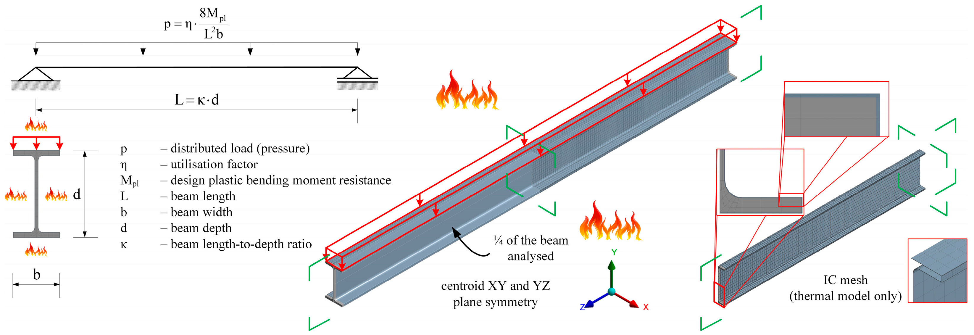
2.1. Thermal and Structural System Scenario

The present numerical study examines a simply supported IPE steel beam subjected to uniform loading. The beam is protected with water-based IC, uniformly covering its entire outer surface with a layer of constant thickness. While subjected to operational loading, the beam is exposed to standard ISO 834 fire from all sides (Figure 1). Due to external heating of the member, the coating undergoes a chemical reaction that activates its thermal insulating function, protecting the substrate material. However, the temperature of the steel beam increases over time, leading to deterioration of the mechanical properties of steel, deformation due to thermal expansion, and a reduction in the load-bearing capacity, ultimately resulting in structural failure.

2.2. Numerical Model Development

2.2.1. Thermal and Structural Model Development

The numerical modelling procedure is developed according to the advanced calculation method provided in EN 1991-1-2 [32] and EN 1993-1-2 [33]. Simulation of structural fire response in ANSYS consists of two sequentially coupled system models. First, thermal response to external temperature variations following the ISO 834 time–temperature fire curve is calculated considering transient heat transfer through conduction, convection, and radiation. A uniform convection coefficient of 20 W/m² °C and an emissivity of 0.95 are applied to all exposed external surfaces. The contact surface between the IC and the steel member is modelled as bonded, assuming there is no relative or sliding motion allowed between them as well as no separation between the contacting surfaces. In order to conduct transient heat transfer analysis, material properties of steel and IC, such as thermal conductivity, specific heat, and density, need to be defined across the full range of expected temperatures. Steel properties are presented in Figure 2, while IC properties are discussed in Section 2.2.2.

In practical scenarios, the structural component would initially undergo deformation as a result of external loading conditions before experiencing additional thermal effects from fire. The latter would necessitate application of a fully coupled thermal–stress model to account for the altered state of the deformed member. However, deformations caused by operational loading are negligible for heat transfer analysis. Therefore, time–temperature profiles are determined based on the undeformed geometry. Temperatures obtained in discrete time increments from the thermal analysis are then transferred as time-dependent body temperatures in the subsequent structural analysis, in which the presence of IC and its contribution to mechanical resistance is omitted.

Following the transient thermal analysis, structural analysis is performed in two steps. First, mechanical load is applied as a uniform pressure along the upper flange surface of the member, corresponding to the predefined level of utilisation. In the second step, while the mechanical load remains constant, the deformed structure with initial pre-stress condition is exposed to thermal loads, transferred from the transient thermal analysis, at specific time intervals throughout the entire duration of the fire. During the iterative simulation process, the analysis is halted once the failure criteria is met.

Since both thermal and structural symmetrical response is ensured by the member’s geometry and loading conditions, two-plane symmetry is applied, which enables modelling only 1/4 of the beam geometry, with appropriate symmetry boundary conditions applied at the member’s centroid (Figure 1). The geometry of the model is discretized using solid FEs with the same mesh in both thermal and structural models. The geometry of the steel profile and IC are discretized using three and four FEs through the material thickness, respectively. As is common for 3D solid structures in ANSYS, FEs used for the thermal analysis are SOLID70 elements, while for the structural analysis, these elements are converted to SOLID185 elements. The adopted time increment is 30 seconds in both thermal and structural analyses. A mesh sensitivity analysis was performed to ensure an optimal balance between computational efficiency and accuracy, confirming that further mesh refinement did not affect the results. Substrate steel material is grade S355, with thermal and mechanical properties modelled according to EN 1993-1-2. The standard ISO 834 fire curve defines a monotonically increasing temperature–time relationship, which leads to a continuous temperature rise in steel elements. As the temperature increases, mechanical properties of steel—including elastic modulus and strength—gradually degrade. Consequently, the material yields, and plastic deformation starts to develop. Since monotonic quasi-static loading is applied, the multilinear isotropic hardening plasticity material model, using the von Mises yield criterion with a yield strength of 355 MPa at ambient temperature, is used. The nominal stress–strain relations dependent on the temperature are converted into true stress–strain relations, presented in Figure 2. The stress–strain curves provided in EN 1993-1-2 implicitly account for the transient creep strain; thus, the effects of transient thermal creep are not considered explicitly. One of the major limitations of implicit models concerns the unloading stiffness at elevated temperatures [34]. Experimental tests on large-scale models have shown that the cooling phase (thermal unloading) is of crucial importance for the behaviour of structures, especially in cases where thermal expansion is restrained, and therefore, the explicit model is particularly recommended when modelling the cooling phase of a fire (parametric and real fire models, which are not covered in this paper).

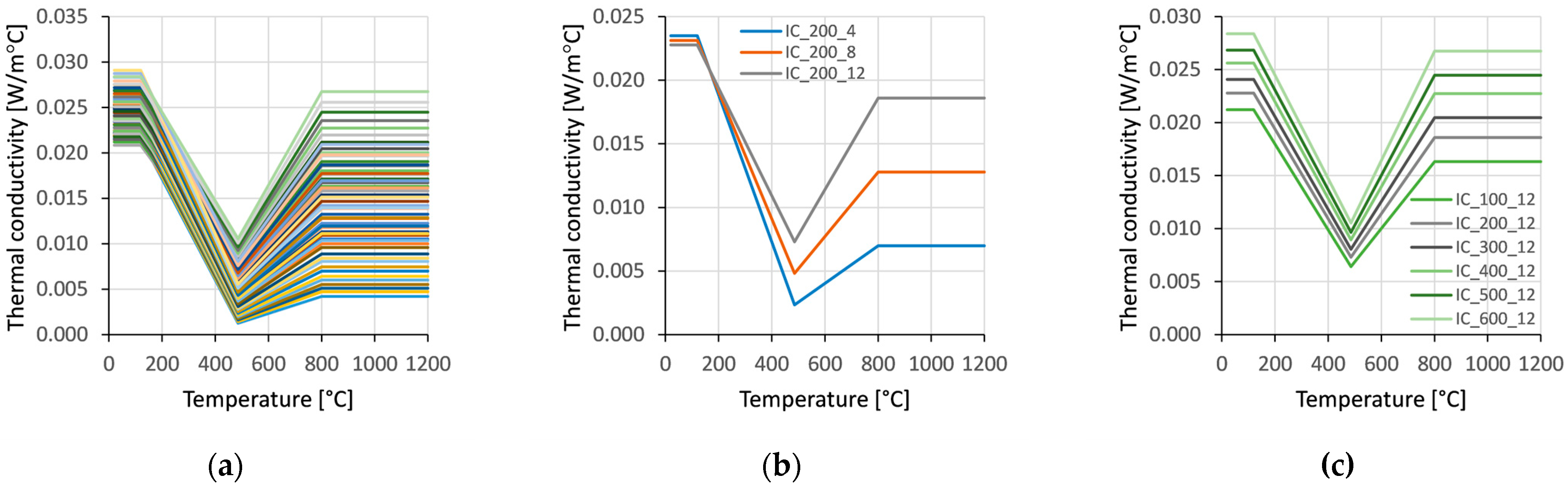
2.2.2. IC Material Model Development

Thermal conductivity is calculated (Equation (1)) according to the standard multivariate linear regression analysis provided by de Silva et al. [30]. The simple formulation given in Equation (1) is considered to be suitable for the issue at hand, being derived from the results of experimental tests on steel plates with water-based IC, while varying the steel plate section factor and the dry IC film thickness.

$${\lambda }_{\mathrm{IC},\mathrm{j}}\left({\mathrm{d}}_{\mathrm{IC}},{\displaystyle \frac{{\mathrm{A}}_{\mathrm{m}}}{\mathrm{V}}}\right)={\mathrm{a}}_0^{\mathrm{j}}+{\mathrm{a}}_1^{\mathrm{j}}{\mathrm{d}}_{\mathrm{IC}}+{\mathrm{a}}_2^{\mathrm{j}}{\left({\displaystyle \frac{{\mathrm{A}}_{\mathrm{m}}}{\mathrm{V}}}\right)}^{-1}$$

(1)

where j refers to the three relevant IC temperature values θ_IC (120, 486, and 800 °C) and a₀, a₁, and a₂ to the regression coefficients presented in

Table 1. Regression analysis coefficients of thermal conductivity function [30].

Coefficient	θIC (°C)
	120	486	800
a0	0.0187	−0.0031	−0.0063
a1	−0.90	6.32	14.50
a2	1.39	0.80	2.02

. Section factor (Am/V) is defined as the ratio between the surface area and the volume per unit length of the steel member. The whole range of IPE profiles is analysed, from IPE600 to IPE80, with section factors ranging from 130 to 430 m⁻¹, respectively. It should be noted that Equation (1) included only section factors of 67, 125, and 250 m⁻¹ [30], while this paper attempts to extrapolate and apply it to a wider geometry range. Lastly, d_IC represents the thickness of dry IC film, including 400, 800, and 1200 µm.

Absolute thermal conductivity function range values of IC, obtained for IPE profiles, as well as the influence of IC thickness and profile section factor, are presented in Figure 3. In the inert phase, equivalent conductivity of IC is in the range of thermal insulation materials. Upon activation, conductivity initially decreases linearly in the transient phase, followed by an increase until reaching a stable phase, where the values are still slightly lower than in the inert phase. The decrease in conductivity is more pronounced in the thinner IC layers, where it stabilizes at significantly lower values than in the inert phase. Additionally, it can be noted that relatively better thermal insulation properties of IC are achieved for higher section factor values, i.e., for smaller profile sections. The specific heat and density of IC are adopted as 1200 J/kg °C and 200 kg/m³, respectively.

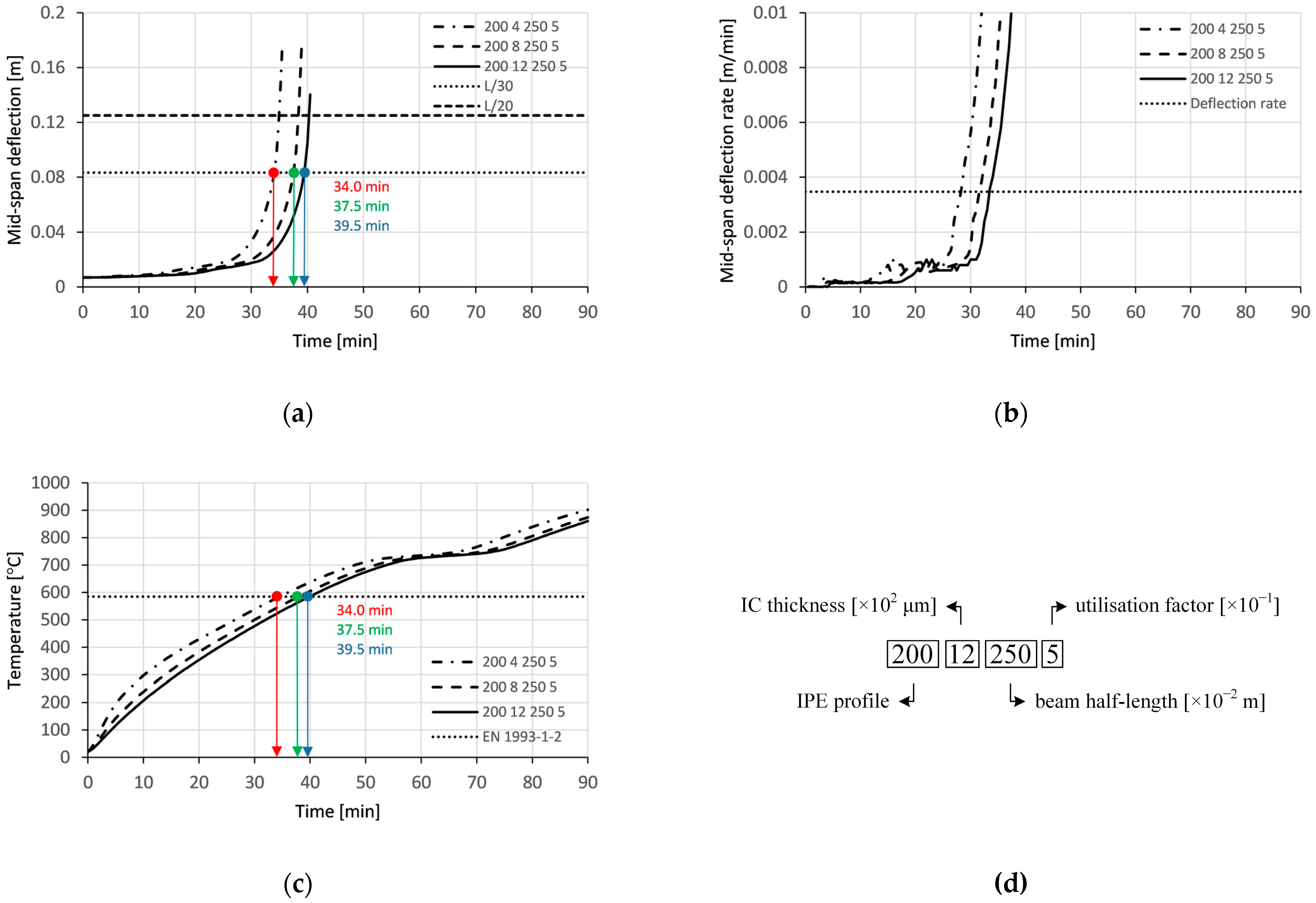
2.2.3. Failure Criteria

The observed beam is considered to have experienced total collapse when the criteria for deflection and deflection rate have been reached [35]. Fire resistance is defined by the duration of fire exposure until failure of the beam. In case of an I-shaped simply supported beam, the failure occurs once the mid-span deflection exceeds L/20 or the rate of deflection exceeds L²/9000 d, where L is the beam span and d is the beam depth. It is highlighted that the rate of deflection is only applicable once the mid-span deflection has exceeded the value of L/30 [36].

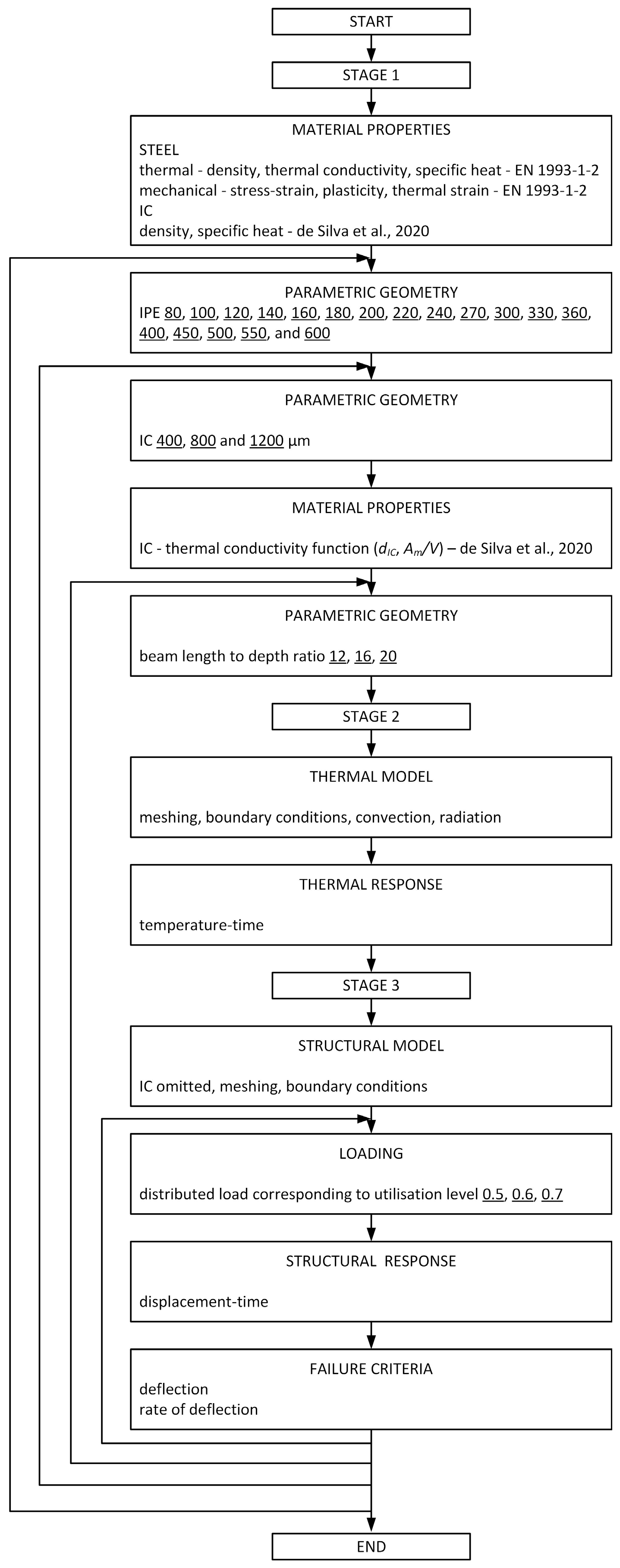
2.3. Parametric Analysis

A simply supported beam is subjected to a uniformly distributed load corresponding to a certain degree of utilisation, defined as the ratio of the stress experienced by the beam under applied loads to the allowable stress the beam can withstand, such as the stress at yield point at ambient temperature. It gives an indication of how close the member is to structural failure [37]. The initial utilisation is 0.5 and its influence on the fire resistance is determined by varying it to the values of 0.6 and 0.7. Beam length is determined in correlation to the observed IPE profile, ranging from 12 to 20 of the corresponding profile depth according to typical application recommendations for beams subjected to bending. The influence of IC on the fire resistance is investigated by varying the dry IC film thickness to values of 400, 800, and 1200 µm. In an attempt to establish the effectiveness of the IC protection, the abovementioned variations of the utilisation, geometry, and IC thickness were employed for the whole range of available IPE steel profiles (80, 100, 120, 140, 160, 180, 200, 220, 240, 270, 300, 330, 360, 400, 450, 500, 550, and 600), amounting to a total of 486 simulations. Methodology of the numerical parametric analysis is presented in Figure 4.

3. Machine Learning

3.1. Artificial Neural Networks

Neural networks are organized in layers, and each layer includes several neurons having an associated activation function [9]. The entire process of training an ANN may be simply described as follows. One input neuron represents one input variable. Each input is multiplied by a corresponding weight, followed by the product summation, and applied to the activation function to form the output value. This scheme is mathematically presented in Equations (2) and (3).

$${\mathrm{u}}_{\mathrm{k}}=\sum ({\mathrm{w}}_{\mathrm{km}}·{\mathrm{x}}_{\mathrm{m}})$$

(2)

$${\mathrm{y}}_{\mathrm{k}}=\mathrm{f}\left({\mathrm{u}}_{\mathrm{k}}+{\mathrm{b}}_{\mathrm{k}}\right)$$

(3)

where x₁, x₂, …, x_m are the inputs; w_k1, w_k2, …, w_km are the synaptic weights of the neuron k; b_k represents bias for the neuron k; function f is an activation function; and y_k is the output value.

Initially, the weights have random values that are adjusted within the training process, during which the relationship between inputs and outputs is gradually detected and finally fixed. An output of one layer “goes through” the activation function and represents the input for the next layer. Activation functions are used for each neuron of a single layer to solve different nonlinear problems [38]. After forwarding the signal through all layers of the network, the transfer function normalizes the output signal and, thus, the output value is obtained. Validation is the intermittent procedure during the training, used to measure generalization of the network and to halt the training process when generalization ceases to improve, indicating that the testing no longer has any effect on the training. Parameters dictating the performance of the network include activation function, number of training iterations, minimum mean squared error, learning rate (how fast the coefficients of regression and weights change), validation check limit, momentum (which is the speed of convergence), number of hidden layers, and number of neurons in each hidden layer.

3.1.1. Dataset

The dataset applied for training, validation, and testing of ANN models includes the results of the parametric analysis (Section 4.2.1) of IPE steel members with IC exposed to standard fire [9]. The input data include detailed beam geometry, thickness of IC, and level of loading (

Table 2. Parameters of the dataset.

Input Neurons	Minimum Value	Maximum Value
H—height of cross-section [mm]	80	600
B—width of cross-section [mm]	46	220
Tw—thickness of web [mm]	3.8	12
Tf—thickness of flange [mm]	5.2	19
r—root radius [mm]	5	24
L—length of beam [m]	1	12
Am/V—section factor [m−1]	129.18	429.32
Nfi—loading factor	0.5	0.7
dIC—thickness of dry IC film [mm]	0.4	1.2
λIC,20 [W/m°C]	0.020858	0.0291
λIC,120 [W/m°C]	0.020858	0.0291
λIC,486 [W/m°C]	0.001243	0.010533
λIC,800 [W/m°C]	0.004205	0.026737
λIC,1200 [W/m°C]	0.004205	0.026737
Output neuron	Minimum value	Maximum value
RT—resistance time [min]	24	53.5

). Output is the fire resistance time expressed in minutes. Fire resistance time is obtained by incorporating conditions of the deflection limit and the deflection rate in the raw data from numerical simulations. The dataset includes all 18 standard types of IPE profiles, three characteristic lengths, three thicknesses of the IC, and three levels of stress loading (utilisation). The geometric parameters are included as separate input neurons instead of only descriptive denominations of IPE size to allow the ability of the neural network to generalize its response for any type of steel S355 I profile within the given geometric range instead of giving the output exclusively for IPE profiles. Processing nodes and their parametric ranges are shown in Table 2. After collecting the data, all values are processed, and numerical values are normalized within the [0,1] interval before employing the dataset for training, validation, and testing of the ANN models.

Additional testing of the ANNs is provided to evaluate the performance of specific models that showed the best behaviour after training within the respective subgroup. To this end, the initial dataset with the min/max range shown in Table 2 has been randomly halved, where one half is used for the repeated training while the other half is used for the evaluation, i.e., testing, of the respective models. It should be noted that both halves of the initial dataset comprehend all IPE profile sizes to provide the most realistic estimate of the models’ performance. The model expressing the best results from each of four subgroups is separately evaluated and compared.

3.1.2. ANN Models

Architecture of the ANN model may influence its response. A way of determining the optimal architecture includes a trial-and-error process. However, ANNs can approximate every continuous function on a compact set to a desired precision. Hence, if provided with a hidden layer containing enough neurons and the sigmoid activation function, it is reasonable to expect a favourable behaviour of the model. This investigation explores the question of optimal architecture with the given algorithm and activation function taking into consideration the size of the dataset. The Levenberg–Marquardt learning algorithm is used because of its fast and stable convergence as well as its suitability for middle-sized networks with up to several hundred weights. This algorithm implies that the training is stopped automatically when the generalization stops improving, which is indicated by an increase of the mean squared error (MSE) of the validation sample. The chosen activation function is unipolar sigmoid (logistic), mathematically described in Equation (4), with logistic form mapping the interval (−∞, ∞) onto (0, 1). Finally, the linear (purelin) transfer function is used at the output layer to transfer the output signal and obtain the final output value. Models are developed using Matlab R2020b [39].

$$\mathrm{f}\left(\mathrm{x}\right)={\displaystyle \raisebox{1ex}{$1$}\!\left/ \!\raisebox{-1ex}{$\left(1+{\mathrm{e}}^{-\mathrm{x}}\right)$}\right.}$$

(4)

A total of 12 models are divided in four subgroups in search for the optimal network architecture. All models have the following parameters: unipolar sigmoid activation function, Levenberg–Marquardt algorithm, one hidden layer, 1000 epoch limit, 10 + 9 momentum, 10⁻⁶ learning rate, and 6-fold cross-validation. Performance is commonly described by the minimum MSE; however, since it is automatically set to 0, the training stops when the network does not improve after six validation checks. Varied parameters are defined as the number of hidden neurons and the subset ratios for training, validation, and testing. The number of hidden neurons is calculated according to Equations (5) and (6) [40]. Additional dependency between the number of input and hidden neurons (Equation (7)) is proposed to investigate if the behaviour of the network would improve or an overfitting of the network would occur when the number of hidden neurons is higher than recommended.

$${\mathrm{N}}_{\mathrm{h}}={\mathrm{N}}_{\mathrm{i}}$$

(5)

$${\mathrm{N}}_{\mathrm{h}}=2·{\mathrm{N}}_{\mathrm{i}}+1$$

(6)

$${\mathrm{N}}_{\mathrm{h}}=3·{\mathrm{N}}_{\mathrm{i}}$$

(7)

Table 3. Nomenclature, architecture, and subsets of ANN models.

Model	Hidden Neurons	Training % (#)	Validation % (#)	Testing % (#)
NN70_10_20-14	14	70 (340)	10 (49)	20 (97)
NN70_10_20-29	29	70 (340)	10 (49)	20 (97)
NN70_10_20-42	42	70 (340)	10 (49)	20 (97)
NN80_5_15-14	14	80 (389)	5 (24)	15 (73)
NN80_5_15-29	29	80 (389)	5 (24)	15 (73)
NN80_5_15-42	42	80 (389)	5 (24)	15 (73)
NN80_10_10-14	14	80 (389)	10 (49)	10 (49)
NN80_10_10-29	29	80 (389)	10 (49)	10 (49)
NN80_10_10-42	42	80 (389)	10 (49)	10 (49)
NN85_5_10-14	14	85 (413)	5 (24)	10 (49)
NN85_5_10-29	29	85 (413)	5 (24)	10 (49)
NN85_5_10-42	42	85 (413)	5 (24)	10 (49)

shows ANN models with their variables. Except for the parameters that are common for all models, there are four sets with varied subset ratios, each including three models with a varied number of hidden neurons, according to Equations (5)–(7). Nomenclature of the models is given in the form NNtr_val_tes-Nh, where tr is the training subset percentage, val is the validation subset percentage, tes is the testing subset percentage, and Nh is the number of hidden neurons. For example, model NN70_10_20-29 represents a network with a subset ratio of 70/10/20 for training/validation/testing with 29 neurons in the hidden layer.

4. Results and Discussion

4.1. Model Verification and Validation

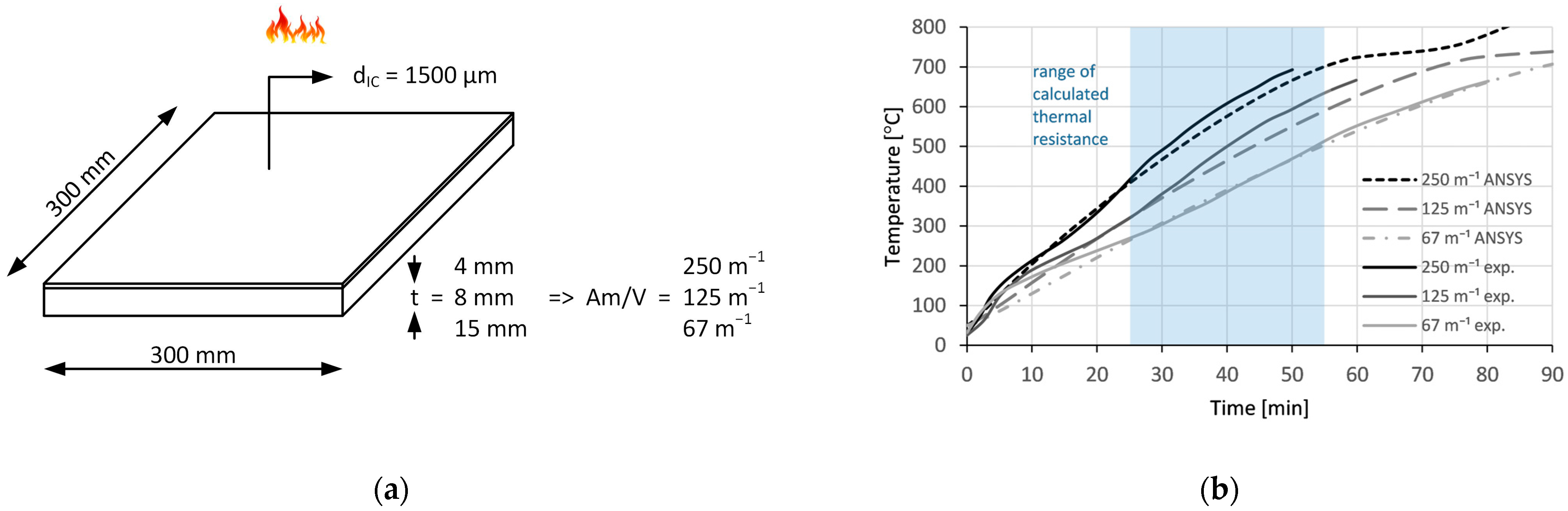
4.1.1. Thermal Model Validation

The thermal model is validated based on experimental data provided by [29] on a group of samples consisting of a steel plate with applied IC with a thickness of 1500 μm on one side of the plate exposed to ISO 834 fire. The plate dimensions are 300 mm × 300 mm with thicknesses of 4, 8, and 15 mm, corresponding to the section factors of 250, 125, and 67 m⁻¹, respectively. Temperature-dependent properties of steel are modelled in accordance with EN 1993-1-2 [33], while the properties of IC are based on [30]. A comparison between experimentally measured temperatures in the plate and numerically obtained temperatures using ANSYS is shown in Figure 5, demonstrating good agreement within the range of fire resistances calculated in this study.

4.1.2. Structural Model Verification

The structural model is verified through multiple stages. Under operational conditions, the normal stress at mid-span is evaluated against the beam’s utilisation factor, ensuring accurate application of a uniformly distributed load at ambient temperature. Fire resistance of the beam is assessed based on the failure criteria outlined in Section 2.2.3. Temperatures at failure are then compared with the critical temperatures specified in EN 1993-1-2 for corresponding utilisation factor values. Figure 6 presents the results of the thermal and structural simulation conducted on an IPE 200 beam with a half-length of 2.5 m, utilisation factor of 0.5, and protected by 1200 μm thick IC layer. Since the rate of deflection criterion is met first but only applies after displacement exceeds L/30, the displacement limit of L/30 indicates the beam’s failure. Figure 7 illustrates the influence of the variation of IC thickness on fire resistance. The evolution of mid-span deflection (Figure 7a) and rate of deflection (Figure 7b) is calculated for IC thicknesses of 400, 800, and 1200 μm. The corresponding failure times in the load-bearing domain are compared with those in the temperature domain (Figure 7c) and further evaluated against the critical temperature thresholds specified in EN 1993-1-2, demonstrating good agreement. Additionally, Figure 7d displays the nomenclature used for the numerical models. Convergence issues were observed in regions of extremely large deformations; however, the structural failure criterion was reached prior to the onset of these issues, indicating that the overall accuracy of the analysis was not compromised.

4.2. Parametric Response

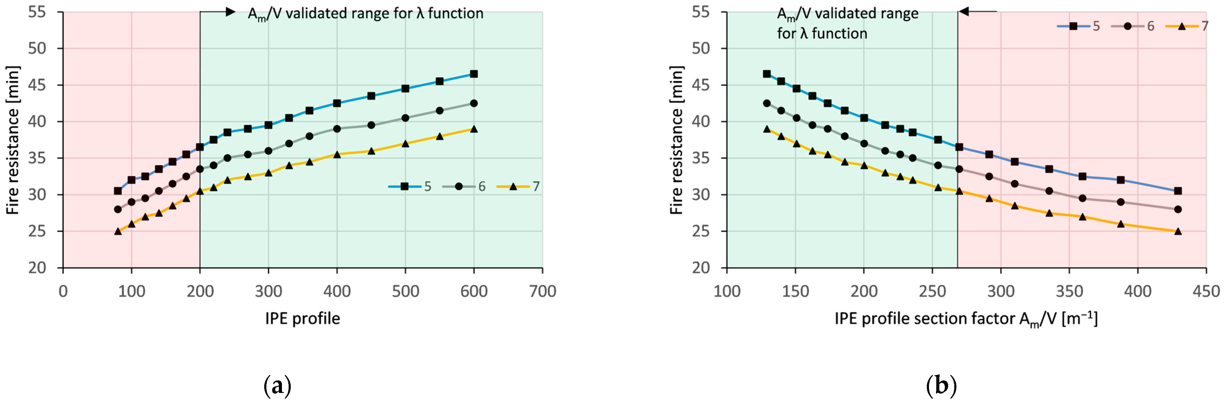
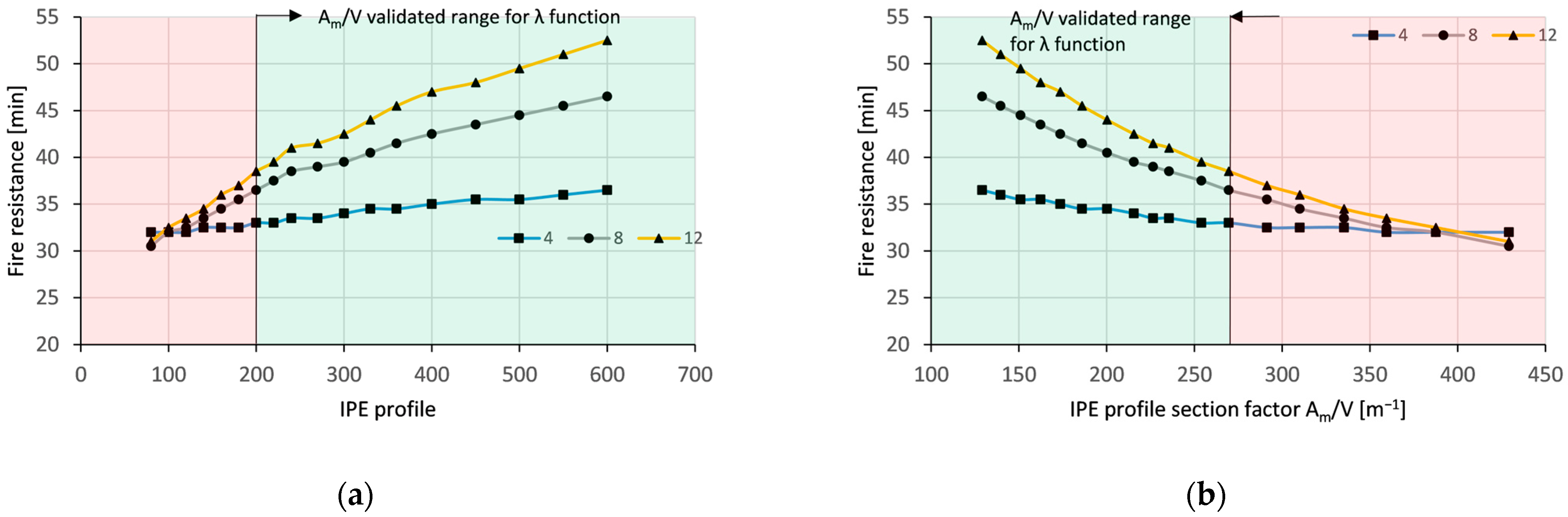
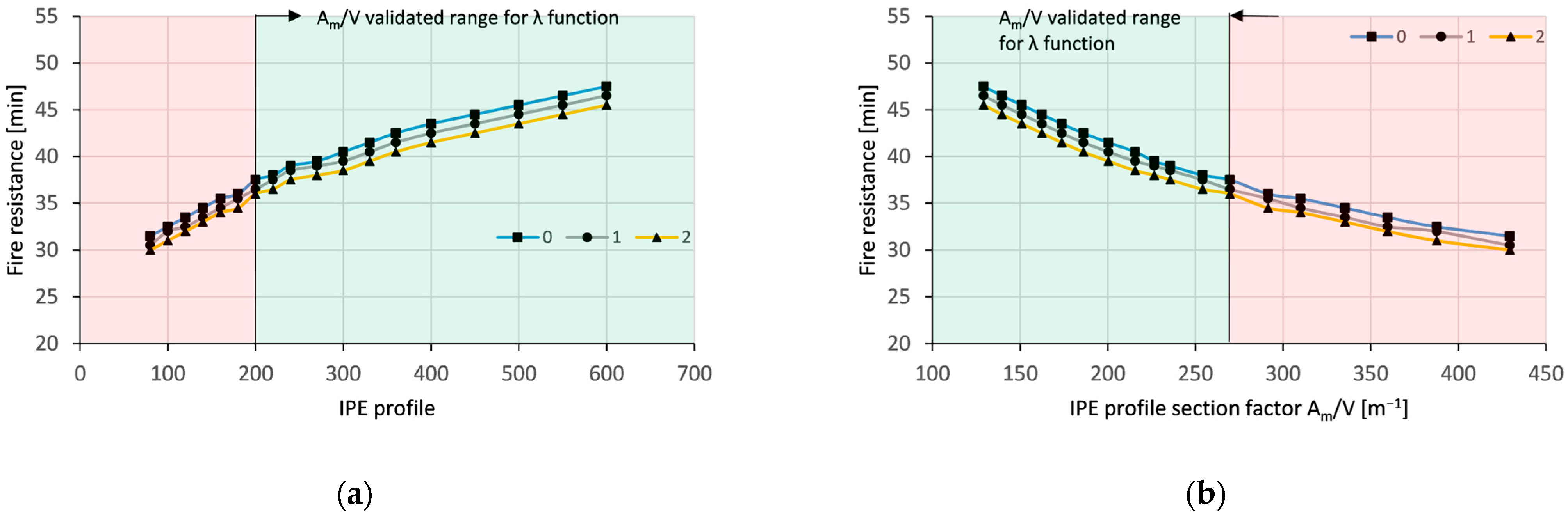
4.2.1. Influence of Beam Section Factor, Utilisation, Length-to-Depth Ratio, and IC Thickness on Beam Failure

Figure 8 presents the fire resistance times for the full range of IPE profiles protected with an IC layer of 800 µm for beam lengths corresponding to 16 times the beam depth and varying utilisation factors of 0.5, 0.6, and 0.7 (denoted as 5, 6, and 7, respectively). As expected, an increase in beam utilisation results in a decrease in fire resistance by approximately 3 to 4 min for every 10% increase in utilisation. The dependency of fire resistance on IC thickness (Figure 9) is shown for a fixed utilisation factor of 0.5; beam length-to-depth ratio of 16; and IC thicknesses of 400, 800, and 1200 µm (denoted as 4, 8, and 12, respectively). The results show that increasing the IC thickness from 400 to 800 µm significantly enhances efficiency compared to the incremental increase from 800 to 1200 µm, considering that the same amount of film is added. Moreover, higher IC thicknesses contribute more to fire resistance for profiles with lower section factors. Figure 10 shows fire resistance in respect to beam lengths equal to 12, 16, and 20 times the profile depth (denoted as 0, 1, and 2, respectively) for the utilisation factor of 0.5 and IC thickness of 800 µm. This indicates that longer beams exhibit slightly lower fire resistance than shorter beams, despite assuming the same thermal response and initial stress levels at the onset of fire.

4.2.2. Limitations of the Mathematical Model with Respect to High Section Factors

As mentioned in Section 2.2.2, the proposed mathematical model was developed based on input parameters obtained through empirical testing within a specific range of section factors. Within this tested range, the model performs with acceptable accuracy. However, when extrapolated to predict the IC thermal conductivity function for higher section factors (particularly beyond 380 m⁻¹), the model yields unrealistic results, including non-physical predictions of reduced fire resistance for thicker IC coatings. These discrepancies highlight the model’s limitations when applied outside the calibrated data range, and therefore, any predictions in this extrapolated domain should be treated with caution. To address this limitation, the proposed methodology suggests extending the experimental testing to include a wider range of section factors. This would provide more robust input data for the regression analysis used to define the conductivity function and enhance the model’s validity across a broader parameter space.

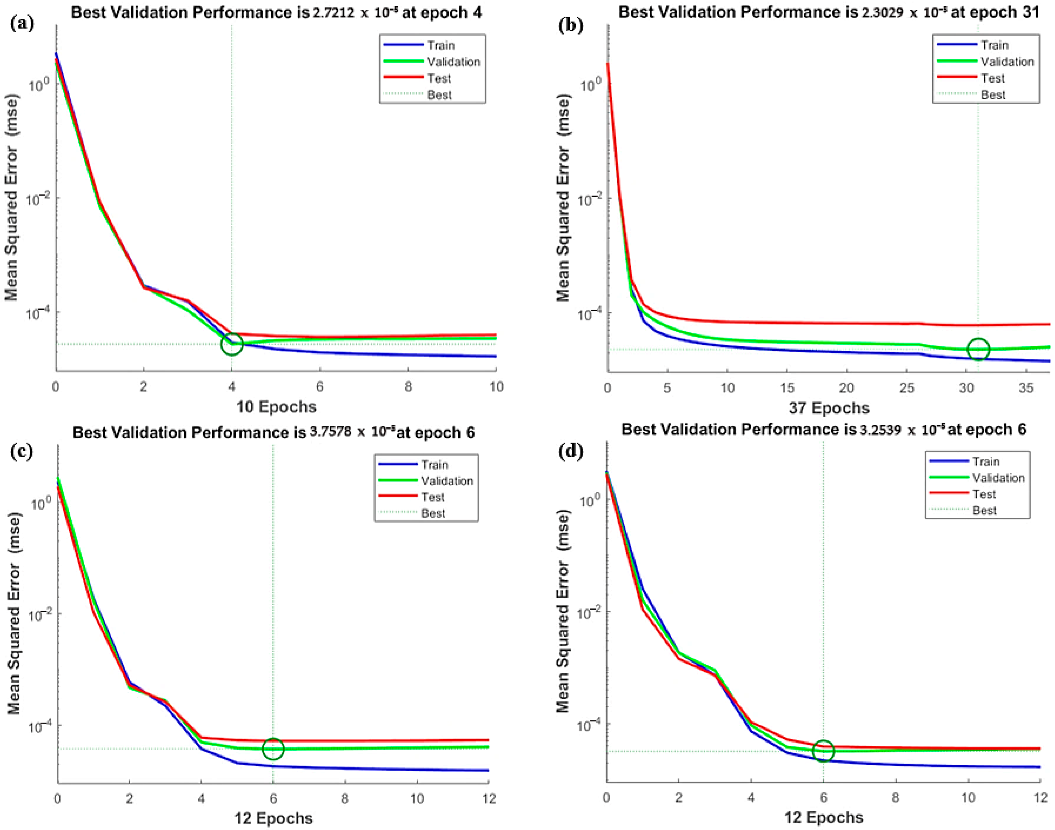
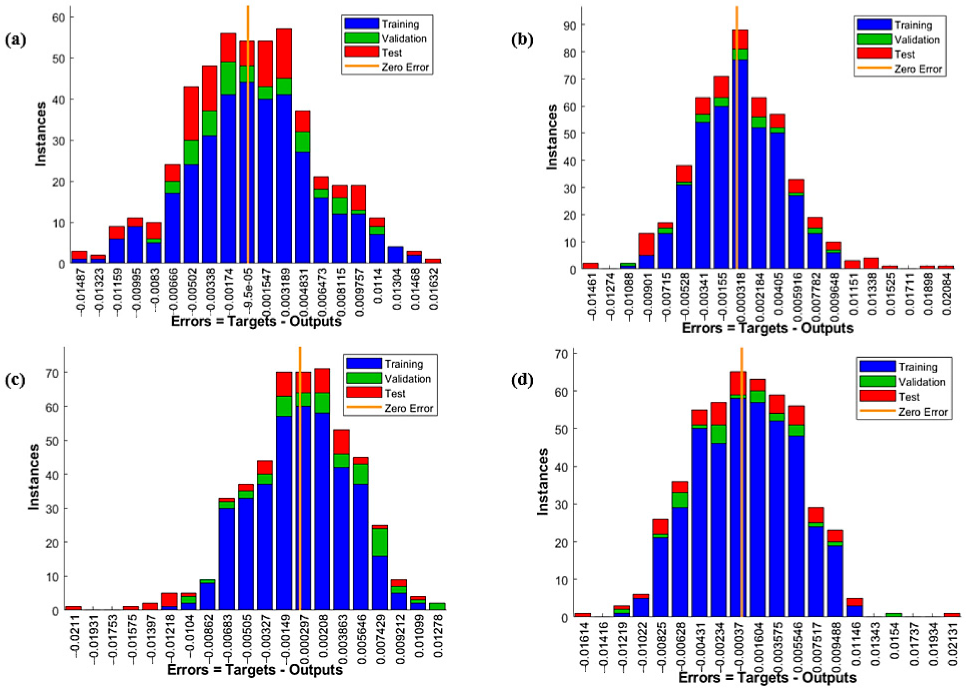
4.3. ANN Models Response

Response of the ANN models is noted by observing the values of regression coefficient (R) and MSE. Coefficient R measures the correlation between output and target values, where the output is the value obtained after training, and the target is the value provided by the dataset. The value of R which tends to 1 represents a very close relationship between the output and target value. The MSE represents the average squared difference between the output and the target values, with the favourable value as close to zero as possible. There are several parameters that affect the performance of a network; however, this work observes the change in the performance depending on the number of hidden neurons and variations of the subset ratio. It is an ongoing discussion on how much responsibility should be assigned to the hidden neurons for the overall error at the output [19]. To get a clearer picture on this matter, factors such as data quality and activation function are constant and, thus, do not influence the results. Responses of all ANN models are presented in

Table 4. Results of the ANN models.

Model	Regression—Training	Regression—Validation	Regression—Testing	Regression—Total	MSE	Epoch
NN70_10_20-14	0.99978	0.99947	0.99951	0.99970	0.0000381	29
NN70_10_20-29	0.99966	0.99975	0.99939	0.99963	0.0000272	10
NN70_10_20-42	0.99977	0.99938	0.99937	0.99965	0.0000440	12
NN80_5_15-14	0.99976	0.99935	0.99950	0.99971	0.0000346	29
NN80_5_15-29	0.99978	0.99977	0.99952	0.99974	0.0000319	23
NN80_5_15-42	0.99981	0.99969	0.99927	0.99972	0.0000231	37
NN80_10_10-14	0.99973	0.99976	0.99950	0.99971	0.0000300	33
NN80_10_10-29	0.99978	0.99963	0.99963	0.99974	0.0000381	36
NN80_10_10-42	0.99977	0.99965	0.99952	0.99971	0.0000376	12
NN85_5_10-14	0.99970	0.99974	0.99910	0.99966	0.0000387	15
NN85_5_10-29	0.99975	0.99949	0.99940	0.99971	0.0000325	12
NN85_5_10-42	0.99984	0.99939	0.99950	0.99978	0.0000485	35

.

Observing the results from

Table 5. Results of the evaluation models.

Model	Training Results						Evaluation Results
	R Training	R Validation	R Testing	R Total	MSE	Epoch	R Total	MSE
EV-NN70_10_20-29	0.99967	0.99908	0.9993	0.9995	0.000077	11	0.9987	0.0017
EV-NN80_5_15-42	0.99993	0.99846	0.9993	0.9998	0.00008	25	0.9983	0.0017
EV-NN80_10_10-42	0.99987	0.99909	0.9977	0.9996	0.000104	11	0.9986	0.0017
EV-NN85_5_10-14	0.99981	0.99968	0.9994	0.9998	0.000024	17	0.9993	0.0016

, models NN70_10_20-29, NN80_5_15-42, NN80_10_10-42, and NN85_5_10-14 stand out with the best behaviour, shown in Figure 11 and Figure 12. These models have regression coefficient values very close to 1, exceedingly low MSE value, and almost regular zero-centred Gaussian distribution of the error between the target and the output values. Table 5 shows that for the lesser number of learning iterations, the regression coefficient is somewhat relatively smaller, which implies stability of the models. From the four models chosen as the optimal for each subgroup, only model NN80_5_15-42 has a relatively high number of iterations followed by the lowest MSE. However, the R value is not the highest of the group, so it may be assumed that the high number of iterations stems from the relatively high number of neurons in the hidden layer. Figure 11 presents the MSE values and progression during the training, validation, and testing stages for the four models, indicating the best of each model group. Quite different behaviour is shown in the first four epochs for all presented models. However, all models show a decreasing trend, whereas the model NN80_5_15-42 shows the smoothest function that continuously decreases until epoch 4, when it starts converging towards zero. Considering that this model had the highest number of epochs, it may be assumed that this allowed for the training to happen in smaller gradual increments, meaning a smaller differential between the weights in each epoch. Figure 12 confirms this assumption, showing that the model NN80_5_15-42 has the most uniform and symmetrical zero-centred distribution, which implies the optimal result. Since it is possible to obtain a false positive result, evaluation models are developed to confirm or otherwise disprove the results of the initial training. Additionally, it should be noted that the hypothesized dependency between the number of input and hidden neurons from Equation (7) shows very good results for the observed architecture with a single hidden layer.

4.4. Evaluation of ANN Models

Evaluation of an ANN model is commonly done by training the network using only part of the dataset and later by testing the same model using the residual part of the dataset. If the error obtained after the evaluation is relatively large, it may signify instability of the model, i.e., that the network is working only for the current dataset, and a proper generalization is probably not achieved, so the network is not giving the same satisfactory behaviour when presented with different data. Hence, additional testing was conducted to evaluate the four models and determine the optimal behaviour after the initial training. As previously mentioned, the initial dataset was halved by a random division, and the obtained sets were used for additional training and evaluation (testing). Table 5 shows the results using a similar nomenclature of the models as for the initial training, with the additional EV marking the evaluation models.

Results of the evaluation show overall good behaviour of all observed ANN models, and only minor discrepancies are observed in comparison to the initial training with the entire dataset. The similarity of the results after training using 50% of the dataset implies that the models are stable and also capable of giving predictions with high accuracy with another dataset. From the four evaluated models, the latter model, EV-NN85_5_10-14, shows almost equal behaviour after both training and evaluation. Additional confirmation is presented through the number of iterations, which is complementary to the initial training, as well as the value of MSE. From the total average results, it may be concluded that model NN85_5_10-14 can be considered as preferable for further use. However, taking into account the overall behaviour presented in Figure 11 and Figure 12, as well as the results of the evaluation, model NN80_5_15-42 shows the best behaviour during training, validation, testing, and evaluation stages.

5. Conclusions

Modelling IC behaviour for the purpose of numerical simulations of structural fire resistance is a challenging process. Complex phenomena occurring in the material can be implicitly accounted for through the implementation of the equivalent thermal conductivity function, dependent on the profile section geometry and the thickness of applied IC as well as temperature. Since coating behaviour varies, experimental data are required for the development of conductivity functions. In the present study, a water-based type of IC used in the study by de Silva et al. [29] was considered for the thermal-structural analysis of a series of IPE beams in fire. The general procedure presented here could also be used for other types of ICs and steel profiles.

Results obtained from the ANSYS analysis of the IPE steel beams protected with IC in fire were used to develop machine learning models for the prediction of fire resistance. Supervised ANN models were developed, and based on the results of conducted analyses, the following conclusions may be drawn:

• Extrapolation of the section factor succeeded to provide appropriate values of thermal conductivity (Equation (1)).
• Efficiency of the applied IC protection is higher for larger profiles, i.e., for lower profile section factors. This is particularly observed for higher IC thicknesses, while in the case of thin IC, the influence of profile size is less pronounced. The fire protection efficiency is not linearly proportional to the thickness of the coating; moreover, it becomes less efficient for higher coating thicknesses.
• As expected, fire resistance depends on the degree of utilisation of the member and is reduced as the utilisation increases.
• In terms of the beam length, practically, minor variations in the fire resistance are obtained, giving preference to the beams with a higher depth-to-length ratio.
• Satisfactory behaviour of all machine learning models confirms a high-quality dataset, implying the suitability of the thermal conductivity function and the rate of deflection limitations that are applied for the parametric analysis.
• The input purposefully included numerical description of the members’ geometry instead of using a simple designation, e.g., IPE80. Therefore, ANN models may be generalized for other types of I steel beams, such as HEA or HEB, for prediction of fire resistance time.
• ANN model NN_85_10_5-14 included 85% of the dataset for training, 10% for testing, and 5% for validation, with 14 hidden neurons. This model showed optimal performance, including good generalization properties after the initial training and after further evaluation. Hence, this model is recommended for the prediction of fire resistance time for I steel profiles with water-based IC in standard fire.

The proposed methodology, along with the developed numerical and predictive ANN models, have the potential to be successfully applied for the structural design of steel in the future, where the required thicknesses of fire protective films, such as IC, can rapidly and in a cost-effective way be estimated to fulfil the fire resistance design requirements of the individual structural elements.

References

1. Hua, Y.; Duan, L.; Zhao, J. Performance-based fire protection of clustered individual members within a steel frame structure. J. Constr. Steel Res. 2024, 218, 108691. [Google Scholar] [CrossRef]
2. Häßler, D.; Hothan, S. Performance of intumescent fire protection coatings applied to structural steel tension members with circular solid and hollow sections. Fire Saf. J. 2022, 131, 103605. [Google Scholar] [CrossRef]
3. Zhang, J.; Guo, Y.; Shao, W.; Xiao, F. Benign design of intumescent fire protection coatings for steel structures containing biomass humic acid as carbon source. Constr. Build. Mater. 2023, 409, 134001. [Google Scholar] [CrossRef]
4. Lucherini, A.; Cristian, M. Intumescent coatings used for the fire-safe design of steel structures: A review. J. Constr. Steel Res. 2019, 162, 105712. [Google Scholar] [CrossRef]
5. Lucherini, A.; Hidalgo, J.P.; Torero, J.L.; Maluk, C. Influence of heating conditions and initial thickness on the effectiveness of thin intumescent coatings. Fire Saf. J. 2021, 120, 103078. [Google Scholar] [CrossRef]
6. Lucherini, A.; Hidalgo, J.P.; Torero, J.L.; Maluk, C. A novel approach to model the thermal and physical behaviour of swelling intumescent coatings exposed to fire. In Proceedings of the 11th International Conference Structures in Fire SiF, Brisbane, Australia, 30 November—2 December 2020. [Google Scholar] [CrossRef]
7. Lucherini, A.; Giuliani, L.; Jomaas, G. Experimental study of the performance of intumescent coatings exposed to standard and non-standard fire conditions. Fire Saf. J. 2018, 95, 42–50. [Google Scholar] [CrossRef]
8. Xu, Q.; Li, G.-Q.; Wang, Y.; Bisby, L. An Experimental Study of the Behavior of Intumescent Coatings under Localized Fires. Fire Saf. J. 2020, 115, 103003. [Google Scholar] [CrossRef]
9. ISO 834-1; Fire-Resistance Tests—Elements of Building Construction—Part 1: General Requirements. International Organization for Standardization (ISO): Geneve, Switzerland, 1999.
10. Gurney, K. An Introduction to Neural Networks, 1st ed.; UCL Press Limited: London, UK, 1997. [Google Scholar]
11. Hammer, B. Neural Networks. In Academic Press Library in Signal Processing; Diniz, P.S.R., Suykens, J.A.K., Chellappa, R., Theodoridis, S., Eds.; Chapter 15; Elsevier: Oxford, UK, 2014; Volume 1, pp. 817–855. [Google Scholar] [CrossRef]
12. Sharma, S.; Sharma, S.; Athaiya, A. Activation Functions in Neural Networks. Int. J. Eng. Appl. Sci. Technol. 2020, 4, 310–316. [Google Scholar] [CrossRef]
13. Kecman, V. Learning and Soft Computing: Support Vector Machines, Neural Networks, and Fuzzy Logic Models, 1st ed.; MIT Press: Cambridge, MA, USA, 2001. [Google Scholar]
14. Shamisi, M.H.A.; Assi, A.H.; Hejase, H.A.N. Using MATLAB to develop Artificial Neural Network for Predicting Global Solar Radiation in Al Ain City—UAE. In Engineering Education and Research Using MATLAB; Chapter 9; Assi, A., Ed.; InTech: London, UK, 2011; pp. 219–238. [Google Scholar] [CrossRef]
15. Gupta, T.; Patel, K.A.; Siddique, S.; Sharma, R.K.; Chaudhary, S. Prediction of mechanical properties of rubberised concrete exposed to elevated temperature using ANN. Measurement 2019, 147, e106870. [Google Scholar] [CrossRef]
16. Tanyildizi, H. Prediction of the Strength Properties Carbon Fiber-Reinforced Lightweight Concrete Exposed to the High Temperature using Artificial Neural Network and Support Vector Machine. Adv. Civ. Eng. 2018, 2018, 5140610. [Google Scholar] [CrossRef]
17. Chaabene, W.B.; Flah, M.; Nehdi, M.L. Machine learning prediction of mechanical properties of concrete: Critical review. Constr. Build. Mater. 2020, 260, 119889. [Google Scholar] [CrossRef]
18. Lazarevska, M.; Cvetkovska, M.; Gavriloska, A.T.; Knežević, M.; Milanović, M. Neural-Network-Based Approach for Prediction of the Fire Resistance of Centrically Loaded Composite Columns. Teh. Vjesn. 2016, 23, 1475–1480. [Google Scholar] [CrossRef]
19. Moradi, M.J.; Daneshvar, K.; Ghazi-nader, D.; Hajiloo, H. The prediction of fire performance of concrete-filled steel tubes (CFST) using artificial neural network. Thin–Walled Struct. 2021, 161, 107499. [Google Scholar] [CrossRef]
20. Quevedo, R.L.; Pardo, Y.L.; Silva, V.P.; Cabrera, Y.F.; Mota, Y.C. Using Numerical Modelling and Artificial Intelligence for Predicting the Degradation of the Resistance to Vertical Shear in Steel—Concrete Composite Beams Under Fire. In Applied Computer Sciences in Engineering, (WEA 2020), Communications in Computer and Information Science; Figueroa-García, J.C., Garay-Rairán, F.S., Hernández-Pérez, G.J., Díaz-Gutierrez, Y., Eds.; Springer: Cham, Switzerland, 2020; Volume 1274, pp. 35–47. [Google Scholar] [CrossRef]
21. Fahmi, A.S.; El-Mandawy, M.E.; Gobran, Y.A. Using artificial neural networks in the design of orthotropic bridge decks. Alex. Eng. J. 2016, 55, 3195–3203. [Google Scholar] [CrossRef]
22. Fu, F. Fire induced progressive collapse potential assessment of steel framed buildings using machine learning. J. Constr. Steel Res. 2020, 166, 105918. [Google Scholar] [CrossRef]
23. Naser, M.Z. Properties and material models for common construction materials at elevated temperatures. Constr. Build. Mater. 2019, 215, 192–206. [Google Scholar] [CrossRef]
24. Han, Z.; Fina, A.; Malucelli, G.; Camino, G. Testing fire protective properties of intumescent coatings by in-line temperature measurements on a cone calorimeter. Prog. Org. Coat. 2010, 69, 475–480. [Google Scholar] [CrossRef]
25. Griffin, G.J. The modelling of heat transfer across intumescent polymer coatings. J. Fire Sci. 2010, 28, 249–277. [Google Scholar] [CrossRef]
26. Bailey, C.G. The behaviour of asymmetric slim floor steel beam in fire. J. Constr. Steel Res. 1999, 50, 235–257. [Google Scholar] [CrossRef]
27. Alam, N.; Maraveas, C.; Tsavdaridis, K.D.; Nadjai, A. Performance of Ultra Shallow Floor Beams (USFB) exposed to standard and natural fires. J. Build. Eng. 2021, 38, 102192. [Google Scholar] [CrossRef]
28. Kolšek, J.; Češarek, P. Performance-based fire modelling of intumescent painted steel structures and comparison to EC3. J. Constr. Steel Res. 2015, 104, 91–103. [Google Scholar] [CrossRef]
29. de Silva, D.; Bilotta, A.; Nigro, E. Experimental investigation on steel elements protected with intumescent coating. Constr. Build. Mater. 2019, 205, 232–244. [Google Scholar] [CrossRef]
30. de Silva, D.; Bilotta, A.; Nigro, E. Approach for modelling thermal properties of intumescent coating applied on steel members. Fire Saf. J. 2020, 116, 103200. [Google Scholar] [CrossRef]
31. ANSYS® Academic Teaching Mechanical. ANSYS Help Documentation, Release 16.0; ANSYS, Inc.: Canonsburg, PA, USA, 2015. Available online: https://www.ansys.com/ (accessed on 1 September 2024).
32. EN 1991-1-2; Eurocode 1: Actions on Structures: Part 1-2: General Actions—Actions on Structures Exposed to Fire. CEN—European Committee for Standardization (ISO): Geneve, Switzerland, 2012.
33. EN 1993-1-2; Eurocode 3: Design of Steel Structures, Part 1-2: General Rules, Structural Fire Design. CEN—European Committee for Standardization (ISO): Geneve, Switzerland, 2012.
34. Gernay, T.; Franssen, J.M. A formulation of the Eurocode 2 concrete model at elevated temperature that includes an explicit term for transient creep. Fire Saf. J. 2012, 51, 1–9. [Google Scholar] [CrossRef]
35. Nguyen, H.L.; Kohno, M. Numerical model of heat transfer for protected steel beam with cavity under ISO 834 standard fire. Fire Saf. J. 2023, 140, 103876. [Google Scholar] [CrossRef]
36. Allam, A.; Nassif, A.; Nadjai, A. Behavior of restrained steel beam at elevated temperature—Parametric studies. J. Struct. Fire Eng. 2019, 10, 324–339. [Google Scholar] [CrossRef]
37. Rackauskaite, E.; Kotsovinos, P.; Jeffers, A.; Rein, G. Computational analysis of thermal and structural failure criteria of a multistorey steel frame exposed to fire. Eng. Struct. 2019, 180, 524–543. [Google Scholar] [CrossRef]
38. Karlik, B.; Olgac, A.V. Performance Analysis of Various Activation Functions in Generalized MLP Architectures of Neural Networks. Int. J. Artif. Intell. 2011, 1, 111–122. [Google Scholar]
39. The MathWorks Inc. Optimization Toolbox, Version: 9.4 (R2022b); The MathWorks Inc.: Natick, MA, USA, 2022. Available online: https://www.mathworks.com (accessed on 1 September 2024).
40. Özturan, M.; Kutlu, B.; Özturan, T. Comparison of Concrete Strength Prediction Techniques with Artificial Neural Network Approach. Build. Res. J. 2008, 56, 23–36. [Google Scholar]
Figure 1. Thermal and structural system and FE mesh of IPE profile and IC.
Buildings 15 02334 g001
Figure 2. Temperature-dependent mechanical and thermal properties of steel S355.
Buildings 15 02334 g002
Figure 3. IC thermal conductivity function range (a), influence of dIC (b) and influence of Am/V (c).
Buildings 15 02334 g003
Figure 4. Block diagram of the numerical parametric analysis.
Buildings 15 02334 g004
Figure 5. Simulated experimental setup (a) and validated thermal response (b) based on [29].
Buildings 15 02334 g005
Figure 6. Verification of the numerical model in load bearing and temperature domain according to EN 1993-1-2 [33].
Buildings 15 02334 g006
Figure 7. Evolution of mid-span deflections (a), rate of deflections (b), temperatures (c), and nomenclature (d) for IPE 200 with 5 m span; utilisation 0.5; and IC thicknesses of 400, 800, and 1200 μm.
Buildings 15 02334 g007
Figure 8. Effect of the degree of utilisation on the fire resistance time as a function of IPE profile (a) and profile section factor (b).
Buildings 15 02334 g008
Figure 9. Effect of the IC thickness on the fire resistance time as function of IPE profile (a) and profile section factor (b).
Buildings 15 02334 g009
Figure 10. Effect of the beam length on the fire resistance time as a function of IPE profile (a) and of IPE profile section factor (b).
Buildings 15 02334 g010
Figure 11. Performance of ANN models during training, validation, and testing for NN70_10_20-29 (a), NN80_5_15-42 (b), NN80_10_10-42 (c), and NN85_5_10-14 (d).
Buildings 15 02334 g011
Figure 12. Error histograms for ANN models with best results: NN70_10_20-29 (a), NN80_5_15-42 (b), NN80_10_10-42 (c), and NN85_5_10-14 (d).
Buildings 15 02334 g012