Critical Review and Benchmark Proposal on FE Modeling for Patch Loading Resistance of Slender Steel Plate Girders in Launched Bridges

Abstract

The patch loading resistance of slender steel plate girders is a critical factor in the design of launched steel and composite steel–concrete bridges. Traditional design methods enhance patch loading resistance through various stiffening techniques, with contributions typically estimated via code expressions calibrated on experimental data that do not always reflect the complexities of full-scale bridge applications. Finite Element (FE) modeling offers a more realistic alternative, though its practical application is often hindered by modeling uncertainties and nonlinearities. To bridge this gap, this paper introduces an advanced FE modeling approach. It provides a comprehensive description of an FE model that accurately predicts both the load–displacement behavior and the patch loading resistance. The model is benchmarked against a broad set of experimental tests and systematically investigates the effects of key modeling parameters and their interactions—material stress–strain law, boundary condition representation, stiffness of the load introduction area, initial geometric imperfections, and solving algorithms. Key findings demonstrate that a bilinear elastoplastic material model with hardening is sufficient for estimating ultimate resistance, and kinematic constraints can effectively replace rigid transverse stiffeners. The stiffness of the load application zone significantly influences the response, especially in launched bridge scenarios. Initial imperfections notably affect both stiffness and strength, with standard fabrication tolerances offering suitable input values. The modified Riks algorithm is recommended for its efficiency and stability in nonlinear regimens. The proposed methodology advances the state of practice by providing a simple yet reliable FE modeling approach for predicting patch loading resistance in real-world bridge applications, leading to safer and more reliable structural designs.

1. Introduction

1.1. Background

Patch loading behavior and resistance on steel-plated structures are of interest to researchers, as together they represent one of the main design constraints on structures subjected to concentrated forces, often more demanding than usual serviceability and ultimate limit states (SLS and ULS, respectively) that the structure must meet. In the typical case of an I-girder, this consists of the instability phenomenon that occurs on the portion of the web plus flange where the patch load is introduced. This failure is governed not only by the plate buckling happening on the web close to the flange but also by the yielding and possible crippling failure of the whole group. Therefore, it represents a combined type of failure. This behavior, depending on the stiffening configuration and geometry, can also be sudden and of high geometric nonlinearity with growing plasticity exacerbated by the geometric nonlinear behavior [1,2].

The most conventional and validated mechanical model to simulate the patch loading behavior is the four-hinges model proposed by Lagerqvist [3,4]. This was later modified by different research contributions that resulted in the formula presented in the first generation of Eurocode 3 for the design of plated structures (EN-1993-1-5:2013) [5] and the subsequent generation (EN-1993-1-5:2024) [6]. As seen, this involved large and extensive research efforts within the European Committee where the COMBRI project [7,8] also contributed to obtaining normatives and guidelines with sufficiently safe designs. To illustrate this, Figure 1 and Figure 2 show the ratio between the predicted ultimate resistance (F_Rd) according to EN-1993-1-5:2013 and EN-1993-1-5:2024 and the real ultimate resistance (F_u) in 413 tests on unstiffened I-girders subjected to pure patch loading. In these figures, the horizontal axis represents the ratio of the applied load length, s_s, to the space between the transverse stiffeners, a. As will be discussed in Section 1.2, these relationships represent part of the main factors influencing the patch loading resistance. The experimental campaigns considered are mentioned in

Table 1. Patch loading tests.

Year	Author, Ref.	Number of Considered Tests
[-]	[-]	[-]
1960	Granholm [9]	7
1977	Drdacky & Novotny [10]	16
1977	Bossert & Ostapenko [11]	10
1978	Rockey [12]	2
1979	Bergfelt [13]	136
1979	Bagchi & Rockey [14]	3
1980	Zoetemeijer [15]	11
1981	Roberts [16]	31
1981	Skolaud & Novak [17]	21
1983	Roberts & Markovic [18]	1
1983	Bamm [19]	4
1983	Bergfelt [20]	18
1987	Galea [21]	1
1987	Shimizu [22,23]	8
1988	Scheer [24]	30
1989	Oxford & Lauger [25]	5
1989	Elgaaly & Nunan [26]	4
1990	Dubas & Tschamper [27]	48
1991	Höglund [28]	2
1991	Dogaki [29]	2
1991	Elgaaly & Sakar [30]	15
1992	Markovic & Hadjin [31]	9
2003	Markovic [32]	6
2007	Gozzi [33]	3
2012	Chacon [34]	3
2018	Kovesdi [35,36]	2
2020	Rogac, Aleksic, Lucic [37]	8
2021	Kovacevic [38]	7

. In both figures, each test is represented by a light gray dot to highlight the overlap of tests between certain ranges.

Typical applications where patch loading resistance is one of the main design constraints are launched structures (bridge construction equipment [39], launched steel or composite concrete–steel bridges [40], and others), industrial cranes, and movable structures (roofs of stadiums, movable floors, etc.). In these examples, it is typical to use longitudinal stiffeners close to the flange where the load is introduced combined with an appropriate spacing between transverse stiffeners and/or diaphragms. However, certain structures—such as bridge construction equipment, e.g., movable scaffolding systems (MSS) [41], and launched bridges—often adopt different stiffening configurations that are not always covered by current code provisions.

1.2. Incremental Launching Method

In the construction of steel and composite steel–concrete bridges, in search of an optimized and economical way to build the deck without interfering with the obstacle that the viaduct crosses, the Incremental Launching Method (ILM) was introduced around the end of the nineteenth century. The first bridges built using this technique were the first Britannia Bridge and the Scorff Bridge (also known as Pont de Lorient sur le Scorff), constructed in the 1850s in Britannia, England, and the 1860s in Nantes, France, respectively [40]. This method is especially suitable in the presence of tall valleys and/or large obstacles and areas where the surroundings of the alignment do not allow the installation of scaffolding or cranes. Furthermore, this technique is not restricted to a specific typology: it has been implemented successfully on cable-stayed bridges, bowstring arch bridges, truss bridges, and typical single/multiple girder configurations such as the Millau bridge in France [42], Arroyo de Las Piedras bridge in Spain[43], and others [39].

The ILM consists mainly of the passage of the bridge along different support conditions until it reaches its final configuration. Normally, one part is partially built on one side of the emplacement and is launched until there is enough space to build the next part, which is then connected to the first. Once these two parts are joined, the whole assembly is moved again until the construction of the next segment is possible. This process continues until the total length of the bridge is built so that the bridge can be placed at its final location. An example of this procedure can be seen in Figure 3. It should be noted that for composite concrete–steel bridges, only the steel structure is usually launched. This is due to the weight of the concrete part. Launching only the steel part considerably reduces the structural demand compared to launching the entire structure.

In specific stages, usually when having the maximum cantilever or unexpected imposed deformations due to construction imperfections, the reaction on the supports has its maximum value. This value later becomes the patch load that represents the limiting design state(s). To solve this problem, structural engineers not only recur to the code provisions to estimate the patch loading resistance but also implement special stiffening techniques such as fully or partially longitudinal and/or transversal stiffening [43,44]. In either of these cases, it is common to find that such code provisions do not comply with the conventional situation of bridges with ILM construction. In the most important singularities of ILM, there is the length of the applied load, also known as s_s in [5,6], the behavior of the temporary supports, and the stiffening strategies applied on the steel structure.

The length of the applied load, s_s, is determined by the bearing material between the temporary launching devices and the bridge deck. These materials typically consist of layered polytetrafluoroethylene (PTFE) and neoprene. This supporting material has admissible pressure loads in both ULS and SLS such that their dimensions are proportional to the acting load. Therefore, it results in large contact areas when it comes to high-load bridge launches. Furthermore, the behavior of these temporary supports depends on their type (rollers, skid-shoes, and others) and the design of their manufacturer. In particular, its stiffness compared to the bridge deck directly affects the distribution of the concentration load. Finally, the stiffening techniques are usually outside the scope of code provisions. In short, the first two directly affect not only the length of the application load but also its distribution, while the third represents techniques that stiffen and strengthen the resistance against concentrated loads or avoid them. An example of an out-of-scope stiffening technique can be seen in Figure 4, where a typical deck configuration, formed by two longitudinal I-girders joined by transverse I-girders, is presented (see in Figure 4a–c). These longitudinal girders are stiffened in the bottom part of the web with a longitudinal triangular-cell stiffening consisting of two plates welded on both the web panel and flanges (see in Figure 4d).

Section 1.1 mentioned the importance of the applied load length, s_s, and the space between the transverse stiffeners, a, in the patch load strength. These are usually observed in dimensionless units by the ratio between them, s_s/a. Similarly influential is the ratio of the distance between transverse stiffeners to the height of the web panel, also called the aspect ratio. This also defines the geometric slenderness of the plate, and it is commonly used in typical problems of buckling for slender plates, e.g., shear buckling [5,6]. In general, the longer the patch load, the higher the resistance [45]. Also, the aspect ratio mostly defines the slenderness and, thus, how prone to buckling the plate is. When classifying the tests in Figure 1 and Figure 2 in terms of the ratios a/h_w and s_s/a, the following can be observed (see gray dots in Figure 5). Should be noted that each of these light gray dots are transparent and become more opaque when overlapping, thus highlighting the tests’ ratios between certain ranges.

First, a large number of tests are particularly focused on small ratios of s_s/a (below 0.4). Furthermore, these tests are of large aspect ratios (up to 20), much larger than those of bridges. To present and compare this, the graphs also include the same ratios of 15 existing bridges built by ILM in the last 25 years in Europe and America (see red dots in Figure 5). A closer look at the main plot (top) is given in the bottom part of Figure 5, specifically for aspect ratios in the range between 0 and 5. The typical loaded lengths of these bridges are between 0.25 and 0.80 times the distance between transverse stiffeners. In addition, the bridge aspect ratios do not exceed 2.50. The minimum value of this ratio is usually constrained by the manufacturing conditions of the steel elements, for example, enough space for welding operations in situ. To exemplify the actual number of tests by the ratios of s_s/a and a/h_w, Figure 6 and Figure 7 introduce the number of tests classified by these ratios.

Figure 6 presents on the vertical axis the number of tests and on the horizontal one the ratio s_s/a, while the red area represents the bridge proportions range previously discussed. Evidently, few tests correctly represent the case of full-scale bridges. This also highlights how the patch load length is an important dimension compared to the horizontal distance between transverse stiffeners. In Figure 7, a similar plot is shown, exchanging the horizontal axis for the value of the aspect ratio, a/h_w. Here the red area also represents the case of the bridges. Two red dashed lines are included, one of which marks the minimum value of the aspect ratio, 0.25, an indicative lower bound in bridges. The maximum value is 4.00, which represents the typical recommended value in steel and composite concrete–steel bridges [46].

As discussed previously, patch loading resistance design values have been considered over the years as sufficiently safe designs in European code provisions. In this context, Eurocodes [5,6] verified the precision of their expressions with experimental campaigns tested in the last 70 years, where they proved to be safe enough (see Figure 1 and Figure 2). However, in the case of launched steel bridges and composite concrete–steel bridges, the number of tests in terms of mechanical and geometric proportions does not represent these situations. Therefore, there is an important component that has not been supported by an adequate number of tests. In this context, Finite Element Method (FEM) models serve as a potential tool that can represent such situations, though their practical application is often hindered by modeling uncertainties and nonlinearities. To bridge the gap between research and practice, this paper investigates their applicability and accuracy in predicting patch loading resistance and behavior. Then, it studies the influence of various modeling strategies on the behavior and ultimate resistance of slender steel elements subjected to patch loading. Finally, this study aims at offering a simple yet reliable benchmark FE model leading to safer and more consistent structural designs.

1.3. Research Methodology

This study followed an experimentally validated numerical approach to investigate the patch loading resistance of slender steel elements and their proper modeling strategies. The main steps of the research methodology were as follows:

-

Selection of relevant experimental campaigns from the literature.

-

Development of a nonlinear Finite Element model capable of capturing key aspects of the structural response, including material and geometric nonlinearity, boundary conditions, and initial imperfections.

-

Calibration and validation of the FE model against experimental results, based on force–displacement curves and ultimate load resistance.

-

Systematic parametric studies using the validated FE model to assess the influence of modeling choices on predicted behavior.

Details of the nonlinear FE model and validation process are provided in Section 2.

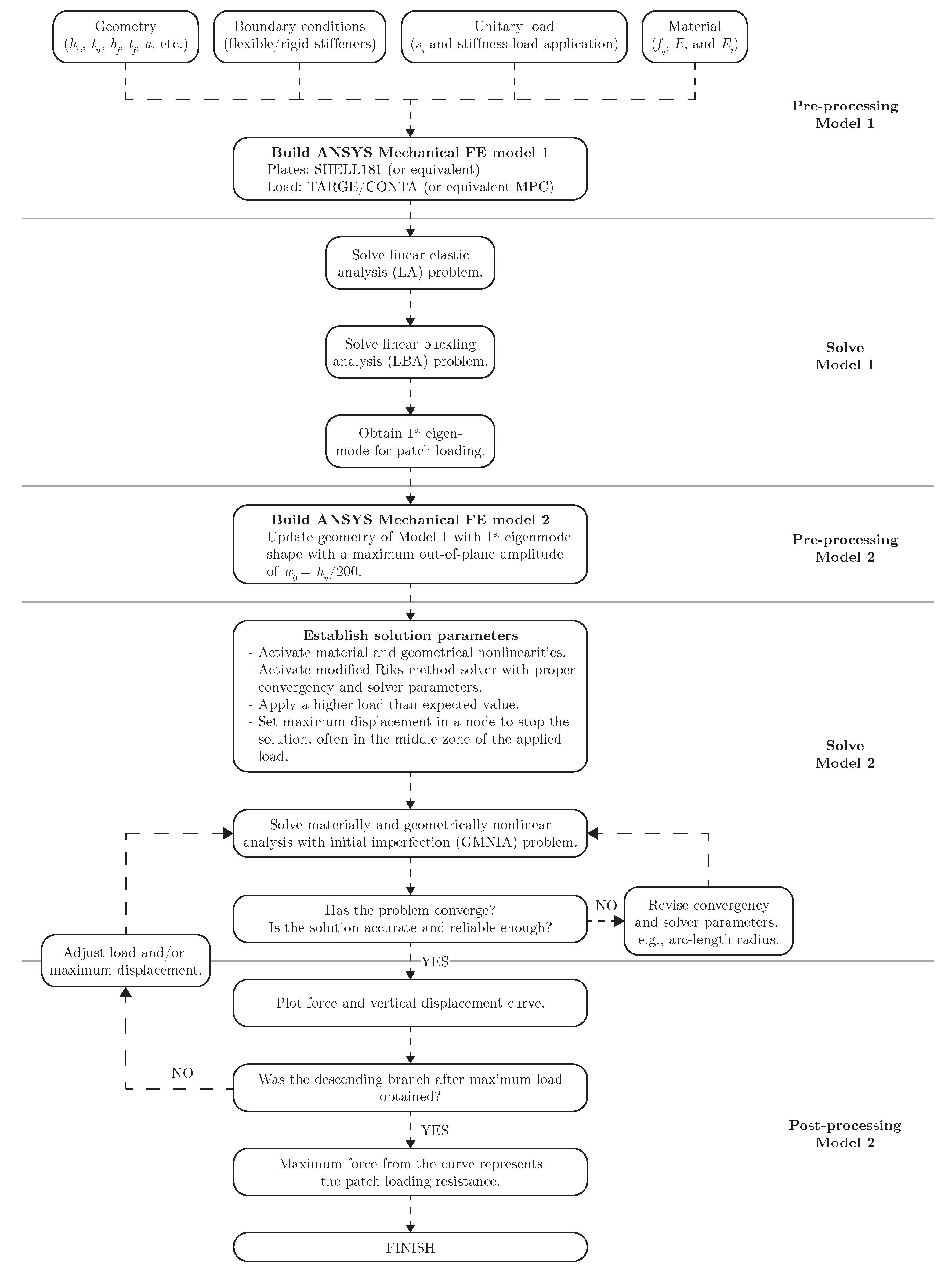
2. Nonlinear Finite Element Model

2.1. Reference Case Studies

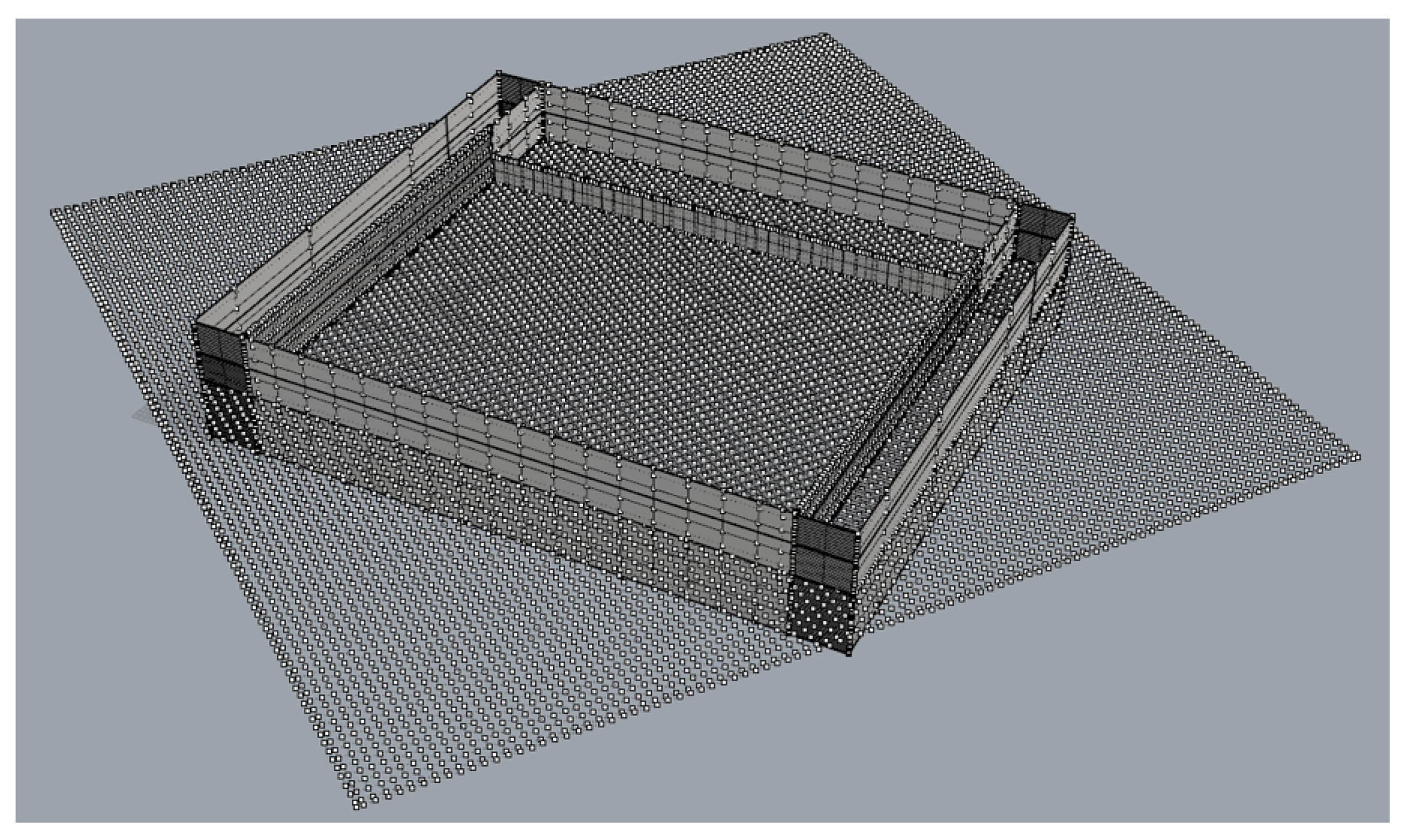
In order to represent the behavior and failure of a plate girder subjected to patch loading, the FEM was used. The type of analysis was Geometrical and Material Nonlinear with Initial Imperfections Analysis (GMNIA). Specifically, three specimens from the literature were selected. These are the P200 and P700 tests from Gozzi (manufactured by Dillinger Hütte in Germany) [33] and the A3 girder from Kovacevic and Markovic (manufactured by Mostogradnja in Belgrade) [38]. These tests were selected because of the detailed information available in the corresponding experiment reports included in the authors’ Ph.D. theses. A brief test summary is included in Appendix B. The modeling strategies in use, which are thoroughly reviewed and criticized in Section 3, provided the most realistic simulation of the tests’ behavior. This is in close connection with current academic FE modeling techniques.

In order to graphically represent each aspect of the FE model, in each of the subsections, what was performed for the A3 girder is introduced. The same procedure applies to the other experiments. The results and the actual test behavior are compared and discussed later. The main dimension variables of importance in the next sections are shown in Figure 8, and the values are presented in

Table 2. Values of dimension on the tests of I-girders subjected to patch loading.

Ref.	Test	tw	hw	fyw	tf	bf	fyf	a	ss	b1	hst	tst	Fu
[-]	[-]	[mm]	[mm]	[MPa]	[mm]	[mm]	[MPa]	[mm]	[mm]	[mm]	[mm]	[mm]	[kN]
[33]	P200	6	1200	371	20	450	354	2440	200	-	-	-	544
	P700	6	1200	371	20	450	354	2440	700	-	-	-	660
[38]	A3	4	500	324	8	120	325	500	50	100	30	8	183

. As seen, these dimension variables were previously mentioned in the first section.

2.2. Description

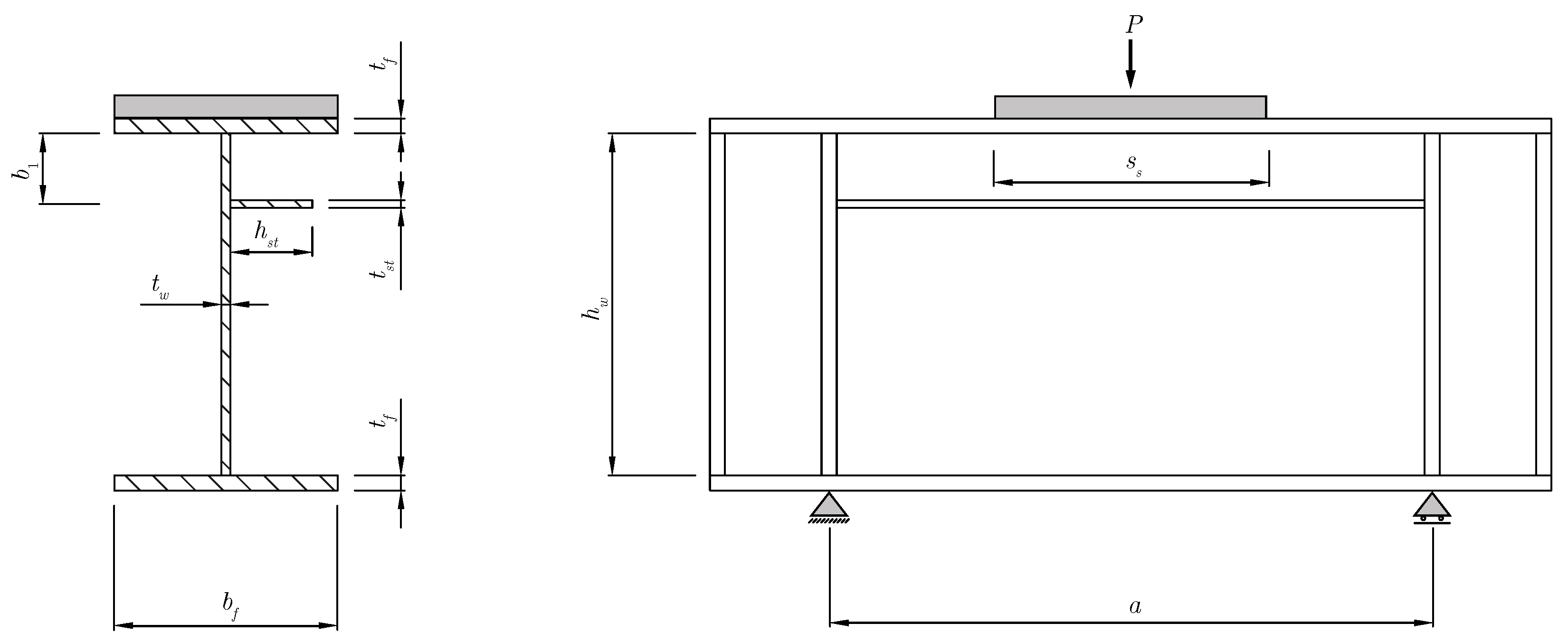
2.2.1. Geometry, Material Properties, and Meshing

Each specimen was modeled to represent the most accurate condition under which they were tested. For this purpose, the software ANSYS^® Mechanical APDL version 2023 R2 [47] was used. The manufacturer is ANSYS Inc. (Canonsburg, PA, USA).

In terms of geometry, each plate is modeled with four-node quadrilateral shell elements with six degrees of freedom (DOF) per node, specifically the SHELL181 from the element library of the program. This element is suitable for analysis with large strains and nonlinear applications. The material was introduced with real stress–strain curves that represent the real plasticity of the tested specimens. This was possible because of the availability of coupon tests on the steel specimens. A mesh sensitivity analysis was used, in which the selected size was close to the thickness of the web panel of each test. This corresponds to common practice in this type of analysis for slender plated steel members [38,45,48,49,50,51].

2.2.2. Boundary Conditions, Load Application, and Analysis

For the boundary conditions, there are three main aspects to be considered. For the following descriptions, U represents the DOF of displacements, and R represents the DOF of rotations. First, as all the tests presented are simply supported, the extremes have restricted the movements in the vertical and transversal directions, UZ and UY, respectively. Second, in the master (loading) node, the rotations in the three axes are restricted: RX, RY, and RZ. Finally, in order to avoid a mechanism in the analysis, the middle bottom point in the web is restricted in the longitudinal direction, UX. These boundary conditions are graphically shown in Figure 9.

The load is applied in a node using multi-point constraints (MPCs), where this node controls the behavior of a group of nodes, assuming a rigid contact. This was simulated in this way given that the tests were conducted with a much stiffer element where the load is applied. To assign the MPCs, the elements TARGE170 and CONTA174 were used to simulate the behavior of the master and slave nodes, respectively. The master node is assigned to the central node of the loaded area where the patch load is introduced, and the slave nodes correspond to the rest of the nodes of the same surface.

In order to obtain the plastic behavior after the highest load that can be resisted, given that it is simulated as a load-controlled test, the modified Riks method was used [52]. This was successfully implemented in ANSYS and proved to work well on buckling problems. Here, a maximum displacement is specified on the master node where the analysis must terminate.

2.2.3. Applied Imperfections

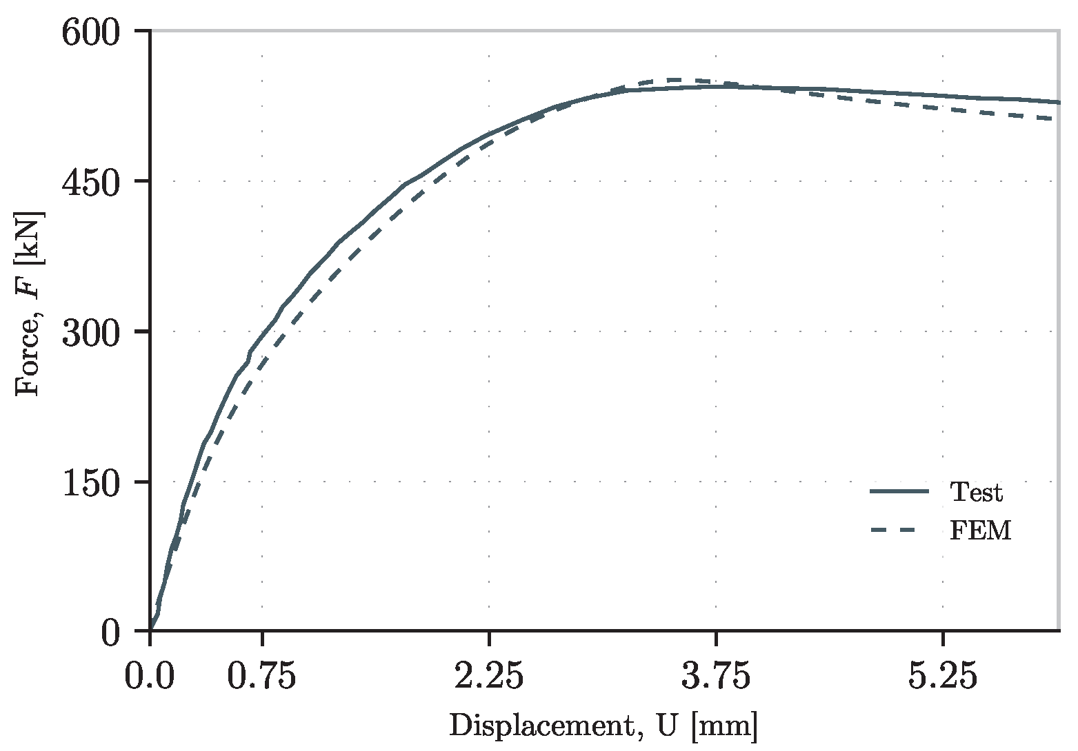
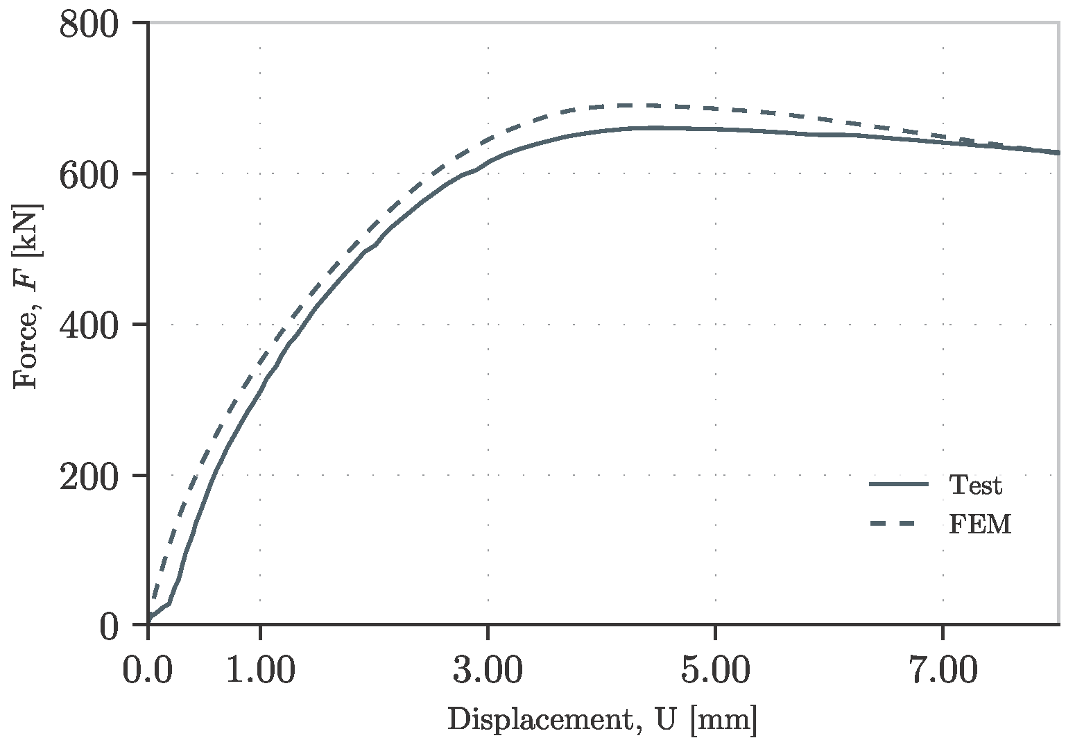
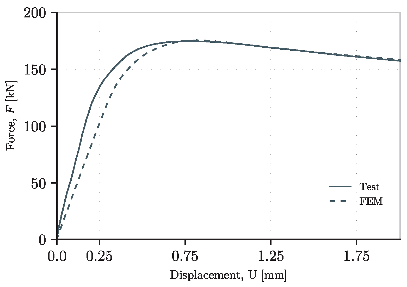
In order to represent the real out-of-plane initial deformation of the web, the contour plots of the initial deformations [38] measured in the web before the test were used. These were introduced in the 3D computer graphics and computer-aided design Rhinoceros [53] to then import the surfaces into ANSYS. The process consisted of first extracting the contours, then generating a grid of points of 10 mm by 10 mm (see Figure 10), and finally creating a surface by quadratic interpolation functions between the points in the two main directions of the plate. This surface was meticulously revised to ensure that the maximum and minimum out-of-plane values remained the same as the initial contour plot. These surfaces were exported as ACIS SAT files and then imported into ANSYS.

For tests where the initial out-of-plane deformation of the web is entirely unknown but the maximum out-of-plane initial imperfection in the mid-span section is known, the shape of the first eigenvalue is used. Once this shape is obtained from a linear buckling analysis (LBA), its maximum value sets the scale value of the whole form. This is the case for P200 and P700 girders [33]. This procedure is explained in more detail in Section 3.

2.3. Validation

To obtain the validation of the FEM model as described above, the results are contrasted in terms of the ultimate resistance and stiffness. Comparing the maximum resistance according to the FEM, there is a maximum error of 5 percent. The exact values per test are shown in

Table 3. Comparison between ultimate load (F_u,test) and FEM simulation (F_u,FEM).

Ref.	Year	Test	ss	ss/a	Fu,test	Fu,FEM	Difference
[-]	[-]	[-]	[mm]	[-]	[kN]	[kN]	[%]
[12]	1978	R1	40	0.05	60	63	+5
		R3	40	0.05	38	41	+9
[27]	1990	VT07	40	0.02	167	165	−1
		VT08	240	0.14	232	255	+10
		VT09	40	0.02	182	186	+2
		VT10	240	0.14	281	303	+8
[33]	2007	P200	200	0.20	544	556	+2
		P700	700	0.70	660	690	+5
[35]	2018	#1	200	0.29	206	215	+4
[38]	2021	A4	25	0.05	180	162	−10
		A3	50	0.10	183	176	−4
		A17	75	0.15	194	202	+4
		A5	100	0.20	225	230	+2
		A6	125	0.25	259	254	−2
		A7	150	0.30	255	292	+14
		B3	50	0.05	165	169	+3
		B5	100	0.10	200	209	+4
		B7	150	0.15	240	251	+4
		B17	150	0.15	234	235	+0
		B4	200	0.20	275	287	+4
		B6	250	0.25	290	314	+8

. The stiffness was well captured in most cases. In the case of the P200 girder, there was a good fit in both the initial stiffness before the ultimate load and after this value. For the P700 girder, there was a shift that potentially meant a movement of the sensor from its original position. If the curve coming from the FE model were to be similarly shifted, the curves would be identical. Finally, for the A3 girder, the model showed stiffer behavior, but the ultimate resistance was well captured. In all three cases, the region after surpassing the ultimate resistance was captured accurately. These results can be seen in Figure 11, Figure 12 and Figure 13.

To profoundly validate this methodology, the results of other FE models in terms of ultimate resistance simulated by the authors are shown. In these models, the same modeling strategies presented were used, and they obtained similar results. This includes some of the tests presented in [12,27,33,35,38]. The results can be seen in a normalized value in Table 3, and the results of the previous tests are bolded (girders A3, P200, and P700). Complete information on these tests can be found in

Table A2. Data of rest of tests used in Section 2.3.

Ref.	Year	Test	a	hw	tw	bf	tf	b1	ss	hst	tst	w0	fyw	fyf	Fu,test	Fu,FEM	Diff.
[-]	[-]	[-]	[mm]	[mm]	[mm]	[mm]	[mm]	[mm]	[mm]	[mm]	[mm]	[mm]	[MPa]	[MPa]	[kN]	[kN]	[%]
[38]	2021	A4	500	500	4	120	8	100	25	30	8	4	321	315	180	162	−10
		A3	500	500	4	120	8	100	50	30	8	3	324	325	183	176	−4
		A17	500	500	4	120	8	100	75	30	8	5.1	318	317	194	202	+4
		A5	500	500	4	120	8	100	100	30	8	5.2	328	321	225	230	+2
		A6	500	500	4	120	8	100	125	30	8	5.6	332	320	259	254	−2
		A7	500	500	4	120	8	100	150	30	8	4	318	317	255	292	+14
		B3	1000	500	4	120	8	100	50	30	8	11.5	315	313	165	169	+3
		B5	1000	500	4	120	8	100	100	30	8	7.14	318	312	200	209	+4
		B7	1000	500	4	120	8	100	150	30	8	19.2	327	339	240	251	+4
		B17	1000	500	4	120	8	100	150	30	8	11	327	339	234	235	+0
		B4	1000	500	4	120	8	100	200	30	8	25	318	323	275	287	+4
		B6	1000	500	4	120	8	100	250	30	8	15.4	262	314	290	314	+8
[35]	2018	#1	1000	500	4	150	10	-	200	-	-	-	286	385	206	215	+4
[33]	2007	P200	2400	1200	6	450	20	-	200	-	-	1.6	371	354	544	556	+2
		P700	2400	1200	6	450	20	-	700	-	-	6.4	371	354	660	690	+5
[27]	1990	VT07	1760	1000	3.8	150	8.35	200	40	90	2	5	375	281	167	165	−1
		VT08	1760	1000	3.8	150	8.3	200	240	90	2	5	358	328	232	255	+10
		VT09	1760	1000	3.8	150	12	150	40	90	2	5	371	283	182	186	+2
		VT10	1760	1000	3.8	150	12	150	240	90	2	5	380	275	281	303	+8
[12]	1978	R1	800	800	2	300	15	-	40	-	-	-	266	295	60	63	+5
		R3	799	800	2	120	5.07	-	40	-	-	5	266	285	38	41	+9

.

3. Modeling Strategies and Discussion

3.1. Introduction

Section 2 was aimed at collecting tests performed by different authors to validate the use of FE models in estimating the behavior and resistance of steel plate girders subjected to concentrated loads. As seen above, the procedure followed is complex and time-consuming, making it difficult to perform in the early stages of the design. Moreover, when designing, there are a considerable number of uncertainties that need to be taken into account when estimating the ultimate resistance. Therefore, in order to simplify all the modeling aspects used before, different approaches that can be applied were selected.

In the following subsections, the influence on the simplification of different aspects of FE modeling is discussed. These are material stress–strain laws, boundary conditions on the panel subjected to the concentrated load, the flexibility on the introduction of the patch load, the magnitude of the initial imperfection, the available solving algorithms, and an example of the combinations of all influencing parameters together. Other influencing parameters such as the application of structural imperfections, i.e., initial residual stresses, are not considered, as other authors proved the negligible influence of these factors on the patch loading resistance [54]. In short, this is explained by the capacity of stress redistribution of the steel. Nonetheless, in the presence of a large magnitude of initial stresses, possibly due to new technologies for steel manufacturing or to specific cross sections with a large amount of welding, special attention and further research must be taken into account [55].

For the following studied cases where individual aspects are analyzed, in order to simplify each case, the P200 girder from Gozzi is used [33]. Additionally, the addressed collapse load is defined as the last load the structure can withstand before failure, corresponding to the last recorded load in the descending branch of the force–displacement curve. Also, the ultimate load refers to the maximum load the girder can sustain, that is, the last recorded load before the descending branch of the force–displacement curve.

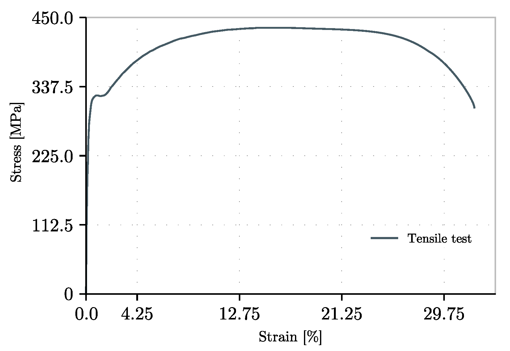
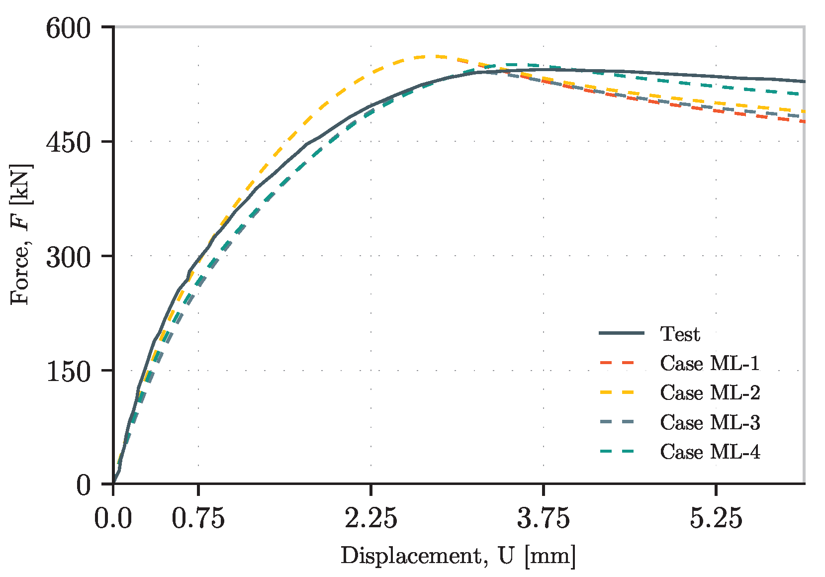
3.2. Material Stress–Strain Law

In the stress–strain law of the material, there can be different configurations. For instance, in Section 2, coupon tests were used. This was only possible due to the availability of this information. Nonetheless, this is not precisely known in early-stage projects and represents the most of what can be known of the material when simulating it. Therefore, other simplifications must be made when designing. It is common practice to use perfect elastoplastic bilinear stress–strain laws for alloy materials such as steel. It must be pointed out that in order to be consistent with the initial validated model, only the material stress–strain law is changed. Therefore, for this case, the following is considered:

-

ML-1: Perfect elastoplastic stress–strain law (Tangent Elastic Moduli, E_t = 0) with the same f_y for all plates.

-

ML-2: Perfect elastoplastic stress–strain law (Tangent Elastic Moduli, E_t = E/1000) with the same f_y for all plates.

-

ML-3: Perfect elastoplastic stress–strain law (Tangent Elastic Moduli, E_t = E/1000) with differing f_y for each plate (flanges and web panel).

-

ML-4: Coupon tests.

These can be considered as different levels of complexity, starting from the most simplistic assumption of the behavior of the material to its real situation. From this, the following can be drawn. These points can be seen graphically in Figure 14 and Figure 15. In the first figure, all the force–displacement curves are drawn, while in the second one, the area represents the filled area between all these options:

-

The use of different stress–strain laws of the material when parting from a completely idealized model, when no further information of the material is given (ML-1), has a sufficient approximation to the ultimate resistance of the girder with a maximum error of +3%.

-

Regarding the initial behavior of the plate in terms of stiffness, the difference between each model is not noticeable until 50% of the ultimate resistance. At this level, the nonlinear behavior governed by the initial stage of the buckling on the web plate behaves differently. For models ML-1 and ML-2, the girder behaves considerably stiffer than the other models. Therefore, the ultimate resistance is higher.

-

The effect of considering a hardening with a slope equivalent to the value of the Elastic Moduli divided by 1000 is only reflected in the post-ultimate load behavior. Moreover, this difference only makes this slope more positive but not in a considerable magnitude (see ML-1 and ML-2 in Figure 14).

-

In order to obtain a behavior closer to the validated model, the yield resistance should be known. This is mainly due to the influence of the yield strength between the flanges and the web on the patch loading resistance [56]. In this case, the force–displacement curve is close to the real behavior until the ultimate resistance. Even at this level, the descending branch cannot be obtained properly.

-

As can be concluded from the previous points, the behavior after passing the ultimate resistance cannot be obtained accurately enough unless the stress–strain law of the steel used is known.

Given that the use of the material model ML-2 gives a closer response in terms of behavior before the ultimate resistance and a close enough approximation of the descending branch after the ultimate load, the next modeling strategies consider this stress–strain law material to obtain an approximation closer to what happens in reality.

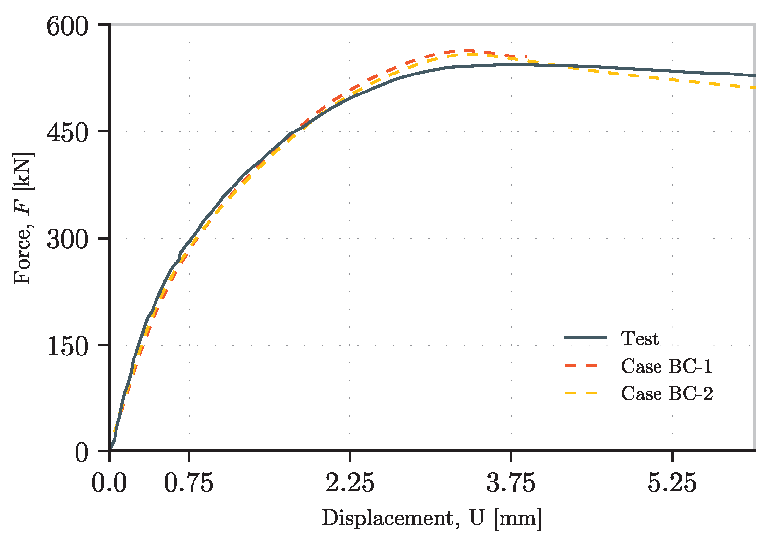
3.3. Boundary Conditions on the Extreme Side of Panels

Regarding the boundary conditions, these refer to the extreme sides of the web panel subjected to the concentrated load. In practical terms, this corresponds to the location of transverse stiffeners. While transverse stiffeners can be explicitly modeled, previous studies [57,58] demonstrated that their effect can be effectively replicated using kinematic constraints (KCs). This approach is particularly advantageous, as transverse stiffeners are usually designed after the web has been dimensioned. The kinematic constraints work only when the transverse stiffeners are very stiff elements. In terms of DOF, this means restraining all the nodes where the transverse stiffener would be positioned, specifically in the vertical direction (direction of the patch load), the out-of-plane direction, and the rotation in the out-of-plane axis. In this subsection, these two strategies of modeling are assessed as follows:

-

BC-1: Using the transverse stiffeners;

-

BC-2: Using kinematic constraints.

As stated above, in this paper it is assumed that transverse stiffeners are designed as rigid transverse stiffeners according to [5,6], not as flexible ones. The behavior of the latter is outside the scope of this paper. Nonetheless, if present, they must be modeled to assess the patch loading behavior or omitted, which would lead to a conservative estimate by underestimating their contribution. From the designated models, the following can be drawn:

-

In terms of stiffness, both models reproduce the same behavior. Therefore, the use of kinematic constraints is accurate enough to successfully replace the transverse stiffeners.

-

In terms of computing time, a considerable amount of time is saved when solving the problem with kinematics constraints instead of the stiffeners. Accordingly, when having more complex structures, this becomes advantageous.

The results can be observed in Figure 16 and Figure 17. In the first figure, all the force–displacement curves are presented, while in the second one, the area represents all these options. As mentioned above, the results are so close to each other that the filled area between both force–displacement curves becomes the same line.

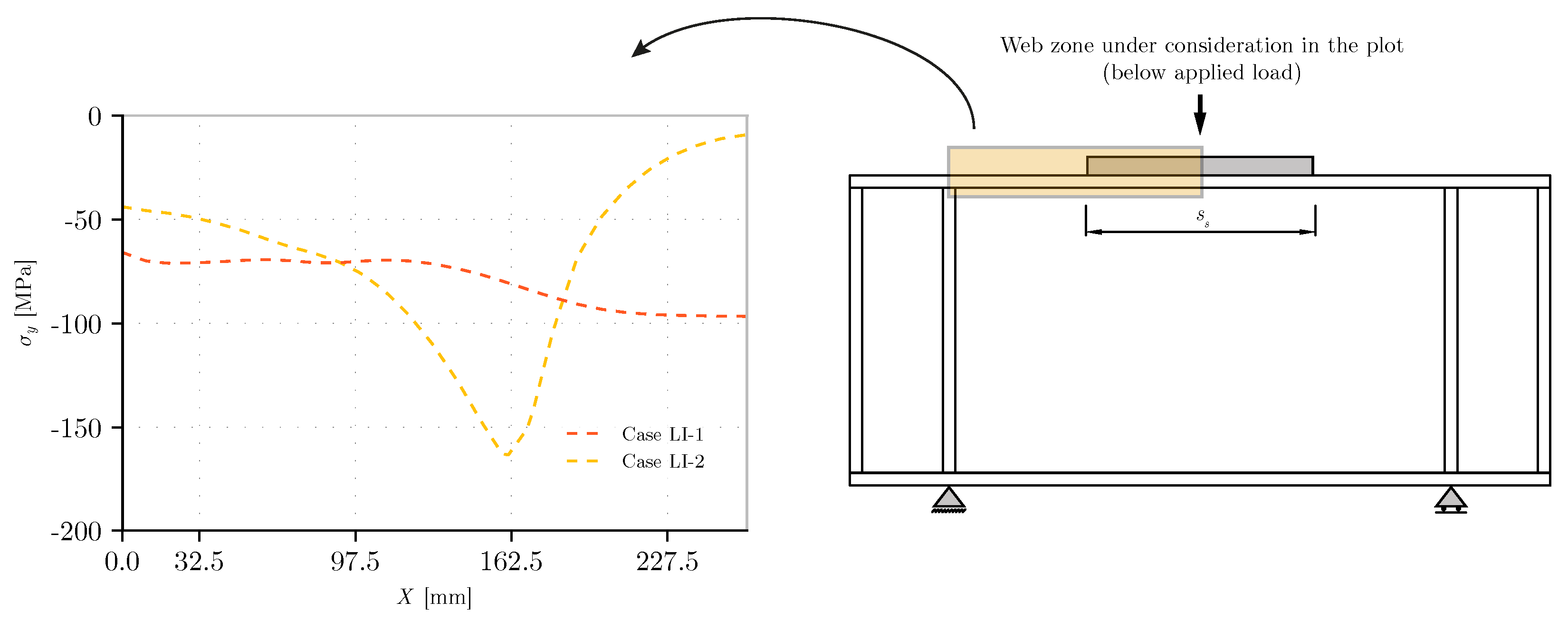
3.4. Introduction of the Concentrated Load

The choice of modeling strategy for the introduction of the concentrated load is an important factor when assessing the patch loading resistance. In real applications, for example, launched bridges (see Section 1.2), the device where the concentrated load acts can be stiffer or more flexible than the cross section of the steel or composite concrete–steel member. This can critically change the ultimate resistance. It does not only affect the load distribution over the web, which can potentially be of a lower length, reducing the ultimate resistance, but it can also be more concentrated on the extremes of the loading device. In these cases, the following occurs:

-

The normal tension on the edges of the load application is considerably higher.

-

The normal tension on the central part of the application load is drastically reduced.

-

In a stiff introduction of the load, one could interpret this as the case of patch loading happening separately on the two edges on a reduced length.

This behavior is graphically represented in Figure 18, comparing load introductions with a stiff and flexible element. In this specific case, a stiff patch loading introduction can increase the normal stress values at the edges of the loaded area by up to twice those observed in a flexible patch loading introduction. Additionally, as expected, the normal stress at the center of the load application remains close to zero for the rigid application element. Therefore, the cases analyzed in this subsection are as follows:

-

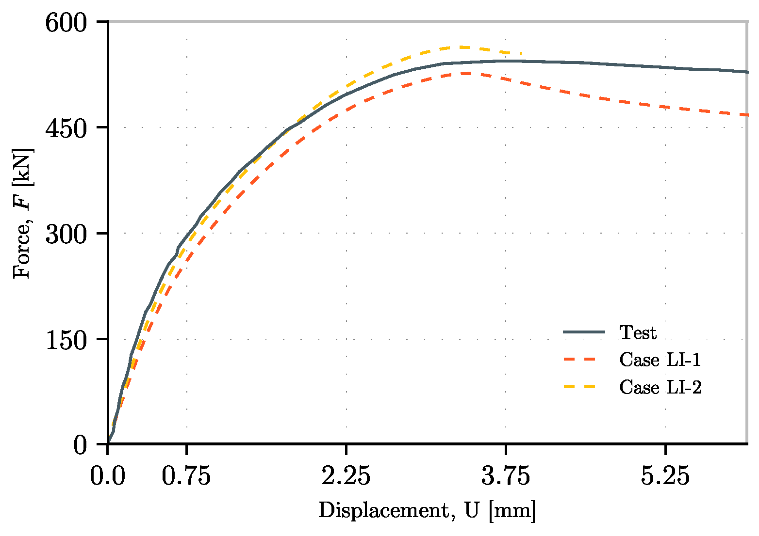
LI-1: Flexible introduction of the concentrated load.

-

LI-2: Stiff introduction of the concentrated load.

The load–displacement curves are presented in Figure 19 and Figure 20.

From these plots, the following can be pointed out:

-

As expected, due to the behavior change when the concentrated load is introduced flexibly, the ultimate resistance is lower. Moreover, its stiffness against the patch load decreases both before and after the ultimate resistance.

-

The introduction of the load with a stiff element can potentially bear a higher load mostly due to the acuteness of the concentrated load on two edges. If F is the patch load applied, F/2 works in a smaller loaded area on each of the edges. Here, three main facts coincide: first, a lower load acting on each of the borders of the loaded area; second, a combination of both loaded areas in further zones of the web; and third, a considerably smaller length of applied patch load. In this case, this results in a higher resistance. Nevertheless, the specific case of each girder must be assessed and analyzed to then be able to understand the results of such higher or lower resistance to patch loading.

-

In this case, the introduction of the load with a flexible element yields a lower resistance due to the reduced application length, s_s, where the total load acts with a parabolic distribution.

-

Consequently, the area between the two force–displacement graphs is larger and considerable. In all cases, it is clear that the influence of the support device stiffness must be assessed with special care.

3.5. Influence of the Initial Imperfection

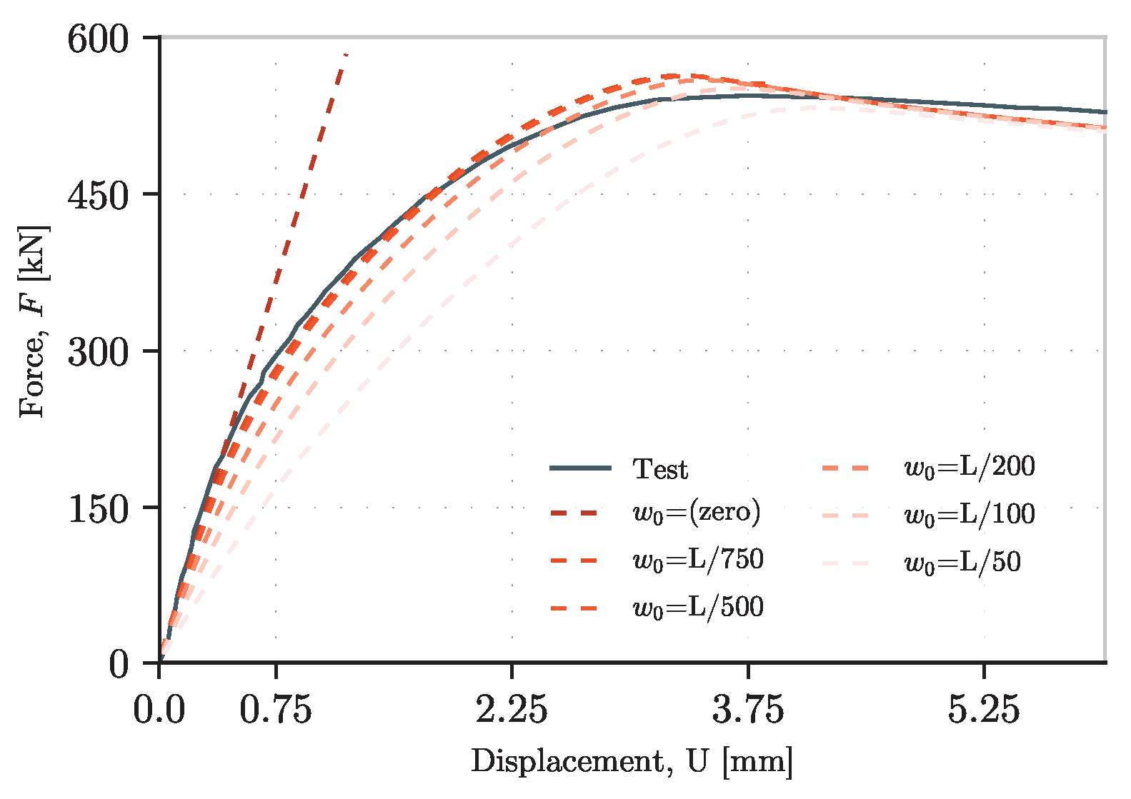
Another relevant parameter is the influence of the initial imperfection. For this case, the shape of the first buckling eigenvalue was used. Herein, it is necessary to solve a Linear Analysis (LA) to be used for the Linear Buckling Analysis (LBA), and thereby obtain the shape. Subsequently, its maximum value is expanded to the value of the selected initial imperfection, w₀. This value is the one that defines the beginning of the geometric nonlinear behavior on the web. An absence of this initial imperfection converts the problem of GMNIA into one of Material Nonlinear Analysis (MNA), as the geometric nonlinear behavior cannot occur. In this case, the load is always centered with the barycenter of the web plate. In reality, this does not occur, even with the most advanced techniques. The plates are not perfect, and they usually include imperfections that occur during manufacturing, transportation, and human error, among others.

In the design of steel structures in Europe, it is common to find this value defined as h_w/200. This value comes from UNE-EN-1090-2 [59], where tolerances for steel plate fabrication and execution are restricted to h_w/100. In the case of other design regulations, e.g., the AISC 360-22 [60], this value is specified as h_w/100. Therefore, the following cases are selected for this study:

-

w₀ = zero.

-

w₀ = L/750, L/500, L/200, L/100, L/50, and L/750, L being the web height of the girder.

From the influence of this value, the following can be said (see Figure 21):

-

In terms of analysis, the case of w₀ equal to zero demonstrated what is mentioned at the beginning of this subsection. The problem becomes one of MNA in the absence of an initial imperfection.

-

In terms of the behavior of the girder, since the magnitude of w₀ controls the geometric nonlinear behavior, the bigger the imperfection, the lower ultimate resistance it reaches.

-

In terms of stiffness, the stiffness logically decreases with the maximum load it can bear. Moreover, the ultimate resistance is lower because of the loss of the girder’s stiffness, mainly influenced by the buckling of the plate. The bigger this imperfection is, the faster the buckling of the web increases, provoking the quicker initiation of the plasticity of the web plate.

-

As stated in the previous points, the choice of the proper initial imperfection, despite the fact that it could be defined in different normatives with different values, directly affects the stiffness and resistance.

-

In experimental campaigns, given the small prototypes that are usually used in laboratories, the values of these imperfections are non-controlled, usually exceeding the values in [59]. This can be seen in an important number of tests similar to those presented in Table 1.

3.6. Solving Algorithms

The use of the proper solver algorithms in the analysis of the GMNIA is up to the user. In these cases, the typical algorithms in nonlinear analysis are tested:

-

SO-1: Modified Riks method [52,61].

-

SO-2: Newton–Raphson procedure [61,62] with displacement-controlled analysis.

-

SO-3: Newton–Raphson procedure [61,62] with force-controlled analysis.

In all of these models, the results are obtained as shown in Figure 22. However, some points to be considered are presented:

-

When using Newton–Raphson with a load-driven analysis (SO-3), it is only possible to obtain the ultimate load depending on the refinement of time steps. Therefore, the final result depends on how small the step is, which, depending on the type of structure, can wind up in a considerably long analysis.

-

When Newton–Raphson is used with a load-driven analysis (SO-3), it is only possible to obtain the force–displacement curve up to the ultimate load. It is not possible to obtain the rest of the curve until the failure of the element (see red dot in Figure 22).

-

When Newton–Raphson is used with a displacement-driven analysis (SO-2), the curve is similar to the one obtained through the modified Riks method. Nevertheless, the refinement of the time steps in the analysis must also be considered in order to obtain the ultimate load accurately. Also, it is possible that nonconvergence of the problem takes place.

-

When using the modified Riks method (SO-1), despite it being a force–driven analysis, it is possible to obtain the whole force–displacement curve. This happens because the refinement is not controlled only by the force; the analysis also depends on a rule of displacement.

-

Regarding computational time, the total solution time for the GMNIA problem in models SO-1, SO-2, and SO-3 is 601, 584, and 603 s, respectively. Among these, models SO-1 and SO-2 exhibit the lowest computational cost, with only a marginal difference between SO-1 and SO-3. However, it is important to emphasize that when using load-driven analysis with the Newton–Raphson method (SO-3), the solution process terminates prematurely as higher load levels cannot be reached, resulting in errors in the solution. Consequently, if the magnitude of the results is entirely unknown, solving the problem would require multiple iterations, each with progressively smaller time steps. In a practical application, this would necessitate at least two iterations of the same problem, effectively doubling the computational cost.

-

In general, when aiming for sufficient accuracy in the force–displacement curve, the modified Riks method provides reliable results with reduced computational time. Moreover, this approach is particularly advantageous in buckling problems, where the web may be susceptible to snap-through behavior, as it helps maintain numerical stability [52].

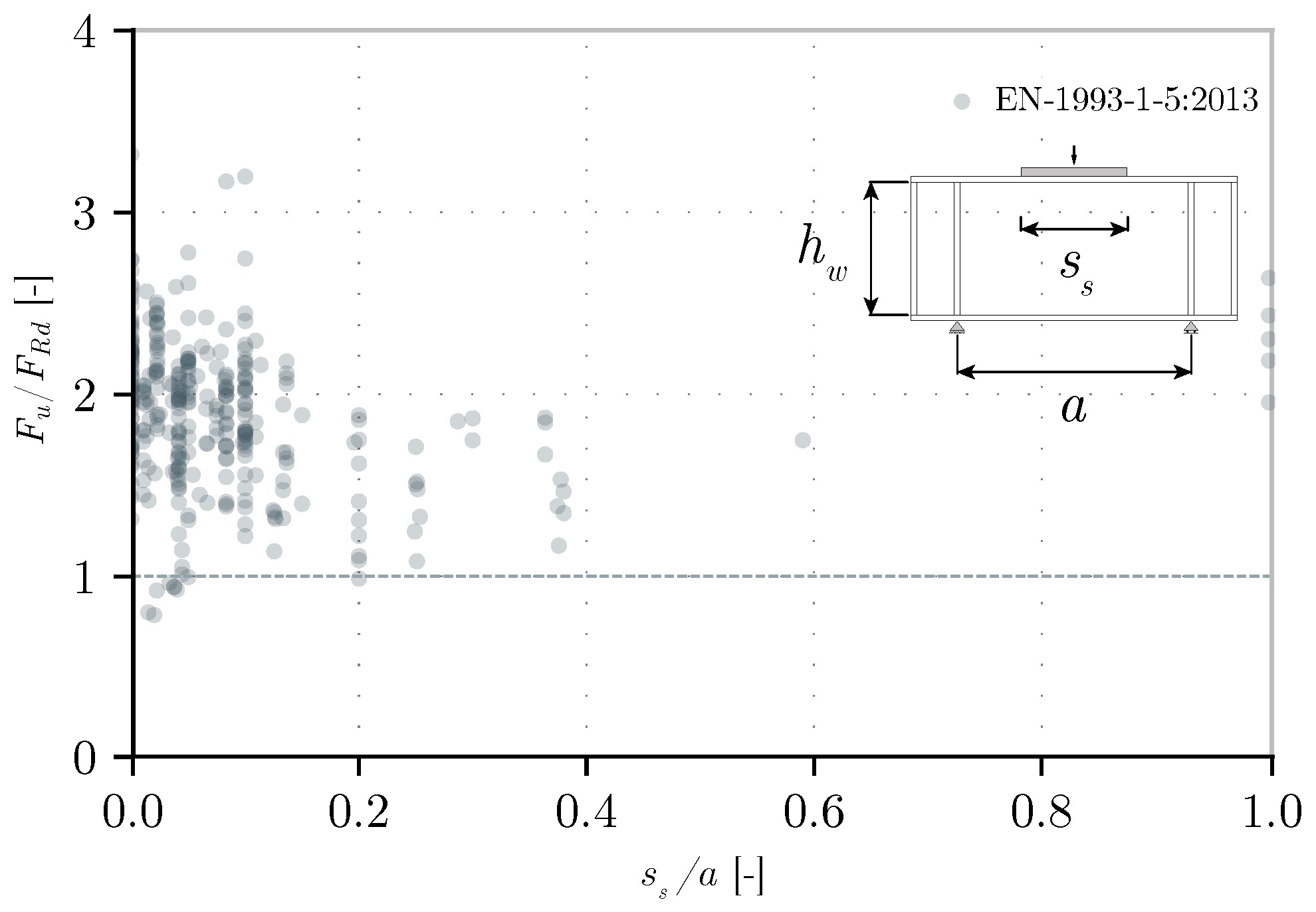
3.7. Combination of Influencing Parameters: From Complex to Simple Models

In the previous subsections, different modeling techniques were analyzed where only one aspect of the FE model was changed to specifically observe the influence of each variable. However, the following subsection examines how different combinations of those techniques can work to estimate the ultimate resistance. In order to perform this appropriately, eleven girders tested by Kovacevic and Markovic [1,38] were chosen due to the information of the steel used and the initial imperfection contour on the web for different tests. From all the tests, a group of single-stiffened girders with an aspect ratio equal to 1 were selected, then another group with an aspect ratio equal to 2. In all these tests, what varies is the length of the applied load. Another important aspect of these tests is that a considerable number of them have a maximum initial imperfection over h_w/200.

In all the modeled cases, the introduction of the load is applied with a stiff element, as that is how the girders were tested. In terms of the rest of the aspects discussed above, five scenarios are defined, where the strain–stress law material, the boundary conditions on extremes, and how the initial imperfections are introduced change. These are described in

Table 4. Combination of modeling techniques.

Model Aspect	CB-1	CB-2	CB-3	CB-4	CB-5
Initial imperfection, w 0	(max. value) a,b	hw/200 a	hw/200 a	Real shape c	Real shape c
Strain-stress law material	ML-2	ML-2	ML-2	ML-2	ML-4
Boundary condition at extremes	BC-2	BC-2	BC-1	BC-1	BC-1

^a The shape of the initial imperfection is the first eigenvalue for patch loading coming from an LBA on which its maximum out-of-plane value is amplified up to the specified value in this table. ^b The maximum value coming from the LBA analysis is amplified to the maximum value measured on the web before the start of the test, i.e., initial scanned geometric imperfections (see Table A2). ^c It corresponds to the shape measured before the test following a procedure like that described in Section 2.2. Here the initial imperfections follows the contour plots.

.

The objective of this section is to present and compare complex modeling techniques, such as the CB-5 model, which combines the most refined techniques, with models such as CB-1 or CB-2, which have very limited information and represent the simplest approach to the structure.

The results of these scenarios are presented in

Table 5. Results for girders with an aspect ratio of 1.

Test	ss	ss/a	Fu,test	Fu,CB-1	Diff.	Fu,CB-2	Diff.	Fu,CB-3	Diff.	Fu,CB-4	Diff.	Fu,CB-5	Diff.
[-]	[mm]	[-]	[kN]	[kN]	[%]	[kN]	[%]	[kN]	[%]	[kN]	[%]	[kN]	[%]
A4	25	0.05	180	153	−15	154	−15	154	−15	152	−16	162	−10
A3	50	0.10	183	166	−9	167	−9	167	−9	170	−7	176	−4
A17	75	0.15	194	190	−2	192	−1	192	−1	199	+3	202	+4
A5	100	0.20	225	209	−7	213	−5	212	−6	229	+2	230	+2
A6	125	0.25	259	237	−8	243	−6	242	−7	254	−2	254	−2
A7	150	0.30	255	256	0	262	+3	262	+3	291	+14	292	+14

for girders with an aspect ratio equal to 1, i.e., the distance between transverse stiffeners is equal to the height of the web. They are also illustrated in Figure 23, showing the difference in terms of percentage, since, x given the difference in terms of force in kilonewtons, the difference is not noticeable. Moreover, to better observe the variation between the models, a pivot chart is shown in Figure 24. Here, the extreme values of each pivot represent the maximum and minimum percentage differences of the ultimate resistance for a given patch load length. In addition, a cross is illustrated that indicates the average of the values found in models CB-1 to CB-5. Finally, a reference line set to zero is defined (the real value of the tests).

From these results, the following can be observed:

-

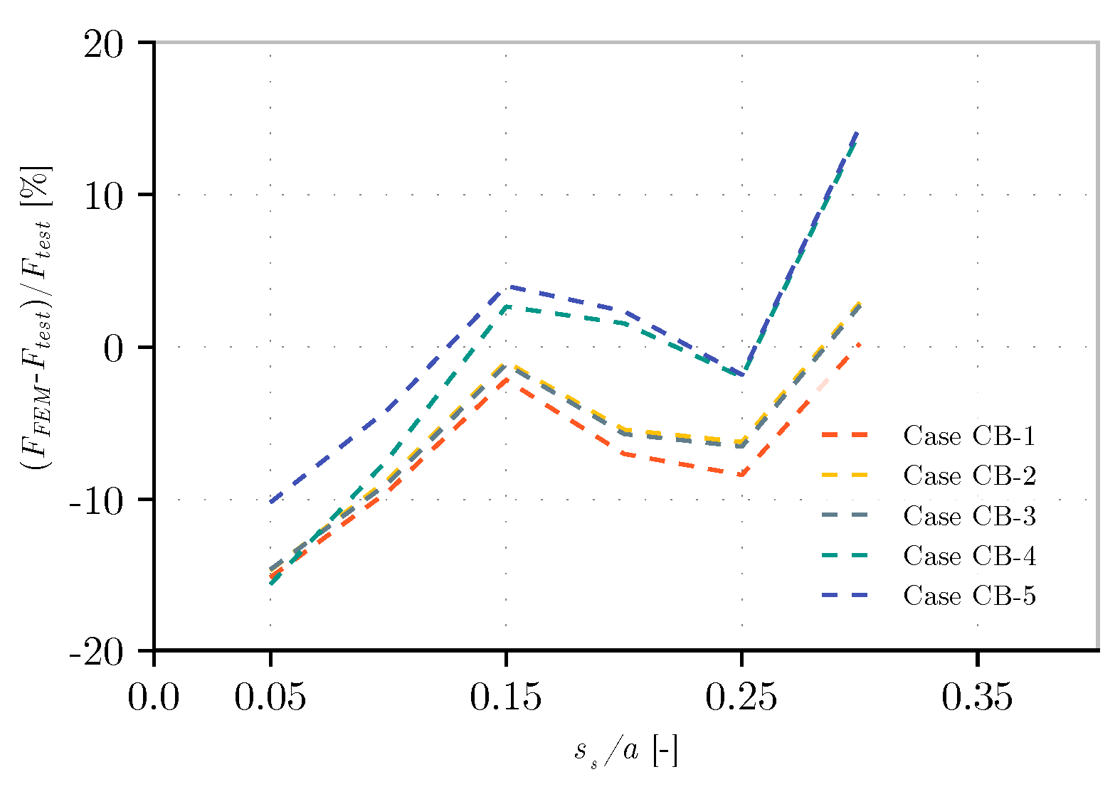
In general, as expected, the results show no large variation. In percentage, they range in value from -16% to +14% of the test value.

-

The worst predictions are encountered in models CB-1 and CB-2, and the best values are found in the most complex model, CB-5. Generally, the most complex model is the one that best approximates the real experimental value but also presents the largest values. The minimum values are found in CB-1. This model, when compared to CB-2, shows lower values due to the magnitude of the initial imperfection which is higher than h_w/200 (see Section 3.5).

-

The difference between models CB-2 and CB-3 is minor. This effect is also found in Section 3.3 when using kinematic constraints or modeling the transverse stiffeners.

-

When using real initial imperfections on the web, at low values of s_s, the effect of the real shape compared to the one of the first eigenvalue is negligible, while at higher values it shows a more pronounced effect. In any of the cases, the last one logically approximates the real behavior of the test.

-

The effect of using the real stress–strain law material is that the results are closer to the real value of the ultimate resistance.

-

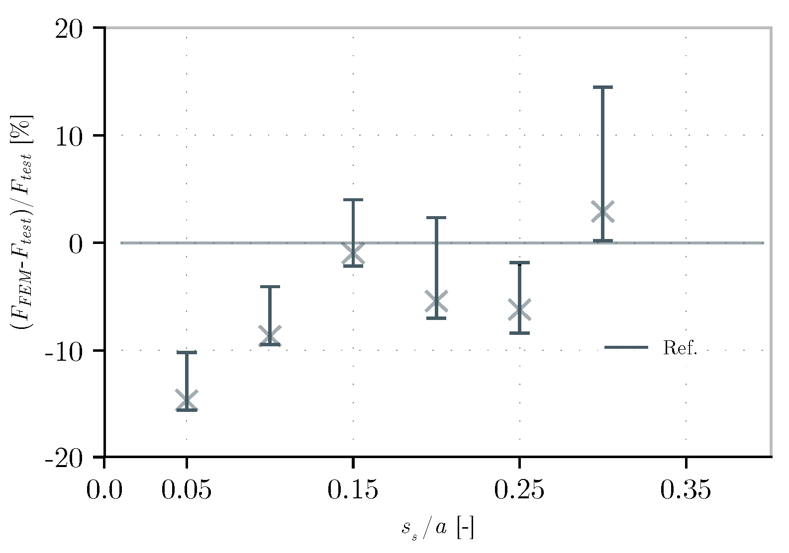
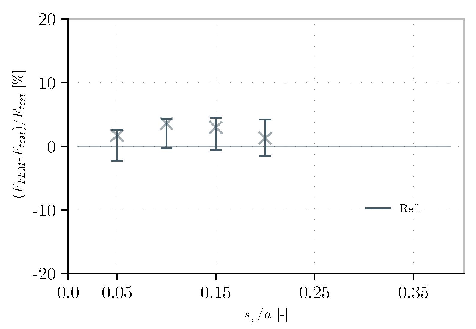
As seen in Figure 24, the average of the values is below the real test resistance, except for the value of the longest patch load. Furthermore, the distance between the lowest and maximum values is similar for most of the tests.

-

For simple models, such as CB-1 or CB-2, it is possible to obtain a good approximation of the ultimate resistance. One of these cases represents the initial model that can be used as a first approximation (CB-2, also following the FEM guidelines according to [5,6]), while the other (CB-1) represents one in which the designer chooses to adopt a conservative assumption by considering a higher value of the initial imperfection.

-

The implementation of complex models such as CB-5 can give a closer approximation to what happens in reality and see other results, such as the force–displacement curve, and strains, among others. Nonetheless, much of this information is not always known in the first stage of design.

In order to fully appreciate what is drawn above, the girders with an aspect ratio of 2 of the specimens from the same author [38] are also modeled. However, in these cases, it is only modeled according to the strategies CB-1 to CB-3 in Table 4. The goal in these models is to see if for another aspect ratio, even when varying the patch load length, it is possible to obtain similar results as the ones obtained previously. These results are found in the same style for the case of an aspect ratio of 1 in

Table 6. Results for girders with an aspect ratio of 2.

Test	ss	ss/a	Fu,test	Fu,CB-1	Diff.	Fu,CB-2	Diff.	Fu,CB-3	Diff.
[-]	[mm]	[-]	[kN]	[kN]	[%]	[kN]	[%]	[kN]	[%]
B3	50	0.05	165	161	−2	168	+2	169	+3
B5	100	0.10	200	200	0	207	+4	209	+4
B7	150	0.15	240	239	−1	247	+3	251	+4
B4	200	0.20	275	271	−1	279	+1	287	+4
B6	250	0.25	290	295	+1	302	+4	314	+8

and Figure 25 and Figure 26.

From these results, the following can be observed:

-

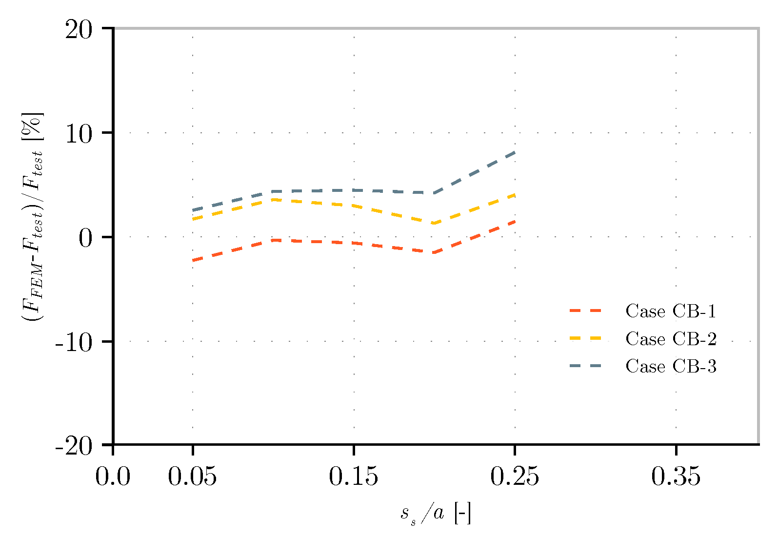
In general, as expected, the results show no large variation and are of a smaller dispersion than the ones with an aspect ratio of 1. In percentage, they range in value from −2% to +8% of the test value.

-

Similar results to the ones of an aspect ratio of 1 are obtained with regard to the initial imperfection and the modeling of transversal stiffeners. That is, the higher the value of w₀, the lower the resistance and the more negligible the effect on the use of kinematics constraints or modeling the transverse stiffeners. In the latter case, not modeling the stiffeners yields conservative results by underestimating their contribution, offering a safety margin.

-

The results between the three types of models show the same hierarchy as the ones with an aspect ratio of 1.

-

Using simple models such as CB-1 to CB-3 can give a sufficient approximation with a small scatter of the ultimate resistance to patch loading.

4. Conclusions

This paper presented and discussed FE modeling strategies for estimating the patch loading resistance of slender steel elements. The following conclusions are addressed:

-

FE modeling is capable of reproducing the force–displacement curve and ultimate resistance of experimentally tested specimens.

-

Simplifications in the material stress–strain law resulted in minimal variation. Therefore, adopting an idealized perfect elastoplastic bilinear model with a hardening branch is sufficient to estimate the ultimate load resistance.

-

The use of kinematic constraints as an alternative to transverse stiffeners, when the latter function as rigid boundary conditions, yields comparable behavior. The difference between these approaches is negligible, which enables the use of simplified boundary conditions in FE models.

-

The stiffness of the element where the concentrated load is applied significantly influences the structural response to patch loading. Thus, a detailed revision is necessary when dealing with flexible or stiff loading elements. In the context of launched bridges, this factor becomes particularly relevant. For cases where the load is applied through a rigid element which represents a large number of tests found in the literature, numerical models effectively replicate the observed behavior.

-

Initial imperfections have a considerable impact on stiffness and strength under patch loading conditions. Specifically, as the initial imperfection, w₀, increases, both stiffness and strength decrease. In this regard, guidelines for defining initial imperfections, aligned with standard tolerances in steel structures, provide appropriate values that can be reliably used in numerical modeling.

-

In terms of solving algorithms, the modified Riks algorithm proves advantageous, not only by achieving sufficiently accurate results with reduced computational effort but also by effectively handling instability problems where snap-through behavior may occur.

-

An FE model incorporating all the proposed simplified modeling techniques has demonstrated sufficient accuracy and precision in predicting patch loading resistance, shedding light on the fact that it is possible to obtain accurate enough results with a simple modeling approach.

-

This study demonstrates that a simplified yet accurate FE model can reliably predict patch loading behavior across a broad range of conditions. Its validated performance enables the extension to cases beyond existing tests, particularly those underrepresented in current standards, supporting both design and further research.

-

To extend the applicability of the benchmark proposal, a validation process similar to that presented in Section 2.3 should be conducted using high-strength steels to verify that it remains effective and accurate for these material types.

-

Future research should investigate the interaction between specific subsets of the modeling techniques explored in this study. Although individual effects and the full combination were evaluated, intermediate combinations could offer deeper insight into the modeling behavior and enhance the robustness of the validation process.

References

1. Kovacevic, S.; Markovic, N. Experimental study on the influence of patch load length on steel plate girders. Thin-Walled Struct. 2020, 151, 106733. [Google Scholar] [CrossRef]
2. Markovic, N.; Kovacevic, S. Influence of patch load length on plate girders. Part I: Experimental research. J. Constr. Steel Res. 2019, 157, 207–228. [Google Scholar] [CrossRef]
3. Lagerqvist, O. Patch Loading: Resistance of Steel Girders Subjected to Concentrated Forces. Ph.D. Thesis, Luleå Tekniska Universitet, Luleå, Sweden, 1995. [Google Scholar]
4. Lagerqvist, O.; Johansson, B. Resistance of I-girders to concentrated loads. J. Constr. Steel Res. 1996, 39, 87–119. [Google Scholar] [CrossRef]
5. EN 1993-1-5:2013; Eurocode 3: Design of Steel Structures—Part 1–5: Plated Structural Elements. The European Committee for Standardization: Bruxelles, Belgium, 2013.
6. EN 1993-1-5:2024; Eurocode 3: Design of Steel Structures—Part 1–5: Plated Structural Elements. The European Committee for Standardization: Bruxelles, Belgium, 2024.
7. COMBRI+. COMBRI Design Manual—Part I: Application of EurocodeRules; Institute for Structural Design: Stuttgart, Germany, 2008. [Google Scholar]
8. COMBRI+. COMBRI Design Manual—Part II: State-of-the-Art and Conceptual Design of Steel and Composite Bridges; Institute for Structural Design: Stuttgart, Germany, 2008. [Google Scholar]
9. Granholm, C. Provning av balkar med extremt tunt liv. Rapport 1961, 202, 1960–1961. (In Swedish) [Google Scholar]
10. Drdacky, M.; Novotny, R. Partial edge load-carrying capacity tests of thick plate girder webs. Acta Tech. CSAV 1977, 222, 614–620. [Google Scholar]
11. Bossert, T.W.; Ostapenko, A. Buckling and Ultimate Loads for Plate Girder Web Plates Under Edge Loading; Fritz Engineering Laboratory: Bethlehem, PA, USA, 1967. [Google Scholar]
12. Rockey, K.C.; Bergfelt, A.; Larsson, L. Behaviour of Longitudinally Reinforced Plate Girders when Subjected to Inplane Patch Loading; Publication S78:19; Chalmers University of Technology, Division of Steel and Timbers Structures: Göterborg, Sweden, 1978. [Google Scholar]
13. Bergfelt, A. Patch Loading on a Slender Web: Influence of Horizontal and Vertical Web Stiffeners on the Load Carrying Capacity; Institutionen för Konstruktionsteknik, Stål-och Träbyggnad: Göterborg, Sweden, 1979. [Google Scholar]
14. Bagchi, D.; Rockey, K. A Note on the Buckling of a Plate Girder Web Due to Partial Edge Loadings; Final Report; International Association for Bridge and Structural Engineering: New York, NY, USA, 1968. [Google Scholar]
15. Zoetemeijer, P. The Influence of Normal-, Bending-and Shear Stresses on the Ultimate Compression Force Exerted Laterally to European Rolled Sections; Stevin Rapport 6-80-5980; Facultiet der Civiele Techniek, Technische Universiteit Delft: Delft, The Netherlands, 1980. [Google Scholar]
16. Roberts, T. Slender plate girders subjected to edge loading. Proc. Inst. Civ. Eng. 1981, 71, 805–819. [Google Scholar] [CrossRef]
17. Skaloud, M.; Novak, P. Post-buckling behaviour and incremental collapse of webs subjected to concentrated loads. In Proceedings of the IABSE, 9th Congress, Amsterdam, The Netherlands, 8–13 May 1972; pp. 101–110. [Google Scholar]
18. Roberts, T.; Markovic, N. Stocky plate girders subjected to edge loading. Proc. Inst. Civ. Eng. 1983, 75, 539–550. [Google Scholar] [CrossRef]
19. Bamm, D.; Lindner, J.; Voss, R.P. Traglastversuche an ausgesteiften Trägerauflagern. Stahlbau 1983, 10, 296–300. (In German) [Google Scholar]
20. Bergfelt, A. Girder Web Stiffening for Patch Loading; Publication S83:1; Chalmers University of Technology, Department of Structural Engineering: Goteborg, Sweden, 1983. [Google Scholar]
21. Galea, Y.; Godart, B.; Radouant, I.; Raoul, J. Test of buckling of panels subject to in-plane patch loading. In Proceedings of the ECCS Colloquium on Stability of Plate and Shell Structures, Ghent, Belgium, 6–8 April 1987; pp. 65–71. [Google Scholar]
22. Shimizu, S.; Yoshida, S.; Okuhara, H. An experimental study on patch loaded web plates. In Proceedings of the ECCS Colloquium on Stability of Plate and Shell Structures, Ghent, Belgium, 6-8 April 1987; pp. 85–94. [Google Scholar]
23. Shimizu, S.; Yabana, H.; Yoshida, S. A new collapse model for patch-loaded web plates. J. Constr. Steel Res. 1989, 13, 61–73. [Google Scholar] [CrossRef]
24. Scheer, J.; Liu, X.; Falke, J.; Peil, U. Traglastversuche zur Lasteinleitung an I-förmigen geschweißten Biegeträgern ohne Steifen. Der Stahlbau 1988, 57, 115–121. (In German) [Google Scholar]
25. Oxfort, J.; Gauger, H.V. Beultraglast von Vollwandträgern unter Einzellasten. Der Stahlbau 1989, 58, 331–339. (In German) [Google Scholar]
26. Elgaaly, M.; Nunan, W.L. Behavior of rolled section web under eccentric edge compressive loads. J. Struct. Eng. 1989, 115, 1561–1578. [Google Scholar] [CrossRef]
27. Dubas, P.; Tschamper, H. Stabilité des âmes soumises à une charge concentrée et à une flexion globale. Constr. Met. 1990, 27, 25–39. (In French) [Google Scholar]
28. Höglund, T. Local buckling of steel bridge girder webs during launching. In Contact Loading and Local Effects in Thin-walled Plated and Shell Structures; Springer: Berlin/Heidelberg, Germany, 1990; p. 135. [Google Scholar]
29. Dogaki, M.; Yonezawa, H.; Kishigami, N. Ultimate Strength Analysis of Plate Girder Webs Under Patch Loading; Elsevier Applied Science Publishers Ltd. (UK): Amsterdam, The Netherlands, 1991; pp. 192–201. [Google Scholar]
30. Elgaaly, M.; Salkar, R. Web crippling under local compressive edge loading. In Proceedings of the 4th National Steel Construction Conference, Washington, DC, USA, 5–7 June 1991. [Google Scholar]
31. Markovic, N.; Hajdin, N. A Contribution to the Analysis of the Behaviour of Plate Girders Subjected to Patch Loading. J. Construct. Steel Res. 1992, 21, 163–173. [Google Scholar] [CrossRef]
32. Markovic, N. Buckling of the Plate Girders Under the Action of Patch Loading. Ph.D. Thesis, University of Belgrade Serbia, Belgrade, Serbia, 2003. [Google Scholar]
33. Gozzi, J. Patch Loading Resistance of Plated Girders-Ultimate and Serviceability Limit State. Ph.D. Thesis, Luleå University of Technology, Luleå, Sweden, 2007. [Google Scholar]
34. Chacón, R.; Serrat, M.; Real, E. The influence of structural imperfections on the resistance of plate girders to patch loading. Thin-Walled Struct. 2012, 53, 15–25. [Google Scholar] [CrossRef]
35. Kövesdi, B.; Mecséri, B.; Dunai, L. Imperfection analysis on the patch loading resistance of girders with open section longitudinal stiffeners. Thin-Walled Struct. 2018, 123, 195–205. [Google Scholar] [CrossRef]
36. Kövesdi, B. Patch loading resistance of slender plate girders with longitudinal stiffeners. J. Constr. Steel Res. 2018, 140, 237–246. [Google Scholar] [CrossRef]
37. Rogač, M.; Aleksić, S.; Lučić, D. Influence of patch load length on resistance of I-girders. Part-I: Experimental research. J. Constr. Steel Res. 2020, 175, 106369. [Google Scholar] [CrossRef]
38. Kovačević, S.D. Stability and Ultimate Capacity of Thin-Walled Steel Plate Girders Subjected to Patch Loading. Ph.D. Thesis, Univerzitet u Beogradu-Građevinski fakultet, Belgrade, Serbia, 2021. [Google Scholar]
39. Members of IABSE Working Group 6. Bridge Deck Erection Equipment; ICE Publishing: London, UK, 2018. [Google Scholar] [CrossRef]
40. Grupo de trabajo 3/10 de la Asociación Española de Ingeniería Estructural. Tableros Empujados; Asociación Española de Ingeniería Estructural: Spain, 2021. (In Spanish) [Google Scholar]
41. Mora Quispe, M.A.; Todisco, L.; Peiretti, H.C. Design Basis of Movable Scaffolding Systems Following American and European Code Provisions and Recommendations. Balt. J. Road Bridge Eng. 2021, 16, 151–177. [Google Scholar] [CrossRef]
42. Virlogeux, M. The Millau cable-stayed bridge. In Recent Developments in Bridge Engineering; CRC Press: London, UK, 2003. [Google Scholar]
43. Millanes Mato, F.; Pascual Santos, J. Viaducto Arroyo las Piedras. Primer viaducto mixto de las Líneas de Alta Velocidad Españolas. Hormigón Acero 2007, 58, 243. (In Spanish) [Google Scholar]
44. Larsen, T.M. Plate Buckling in Movable Scaffolding Systems. Master’s Thesis, University of Oslo, Oslo, Norway, 2011. [Google Scholar]
45. Ceranic, A.; Bendic, M.; Kovacevic, S.; Salatic, R.; Markovic, N. Influence of patch load length on strengthening effect in steel plate girders. J. Constr. Steel Res. 2022, 195, 107348. [Google Scholar] [CrossRef]
46. Ministerio de Fomento. Instrucción de Acero Estructural (EAE); Boletín Oficial del Estado (BOE); Ministerio de Fomento: Madrid, Spain, 2012. (In Spanish) [Google Scholar]
47. ANSYS Inc. Ansys Mechanical APDL, Version 2023R2. [Software]. Canonsburg, PA, USA, 2023.
48. Chacón, R.; Mirambell, E.; Real, E. Influence of flange strength on transversally stiffened girders subjected to patch loading. J. Constr. Steel Res. 2014, 97, 39–47. [Google Scholar] [CrossRef]
49. Graciano, C.; Casanova, E.; Martínez, J. Imperfection sensitivity of plate girder webs subjected to patch loading. J. Constr. Steel Res. 2011, 67, 1128–1133. [Google Scholar] [CrossRef]
50. Chacón, R.; Mirambell, E.; Real, E. Hybrid steel plate girders subjected to patch loading, Part 1: Numerical study. J. Constr. Steel Res. 2010, 66, 695–708. [Google Scholar] [CrossRef]
51. Demari, F.E.; Mezzomo, G.P.; Pravia, Z.M.C. Numerical study of slender I-girders with one longitudinal stiffener under patch loading. J. Constr. Steel Res. 2020, 167, 105964. [Google Scholar] [CrossRef]
52. Riks, E. An incremental approach to the solution of snapping and buckling problems. Int. J. Solids Struct. 1979, 15, 529–551. [Google Scholar] [CrossRef]
53. Robert McNeeel; Associates. Rhinoceros 3D, Version Rhino 6, [Software]; Seattle, WA, USA, 2018.
54. Chacón, R.; Mirambell, E.; Real, E. Influence of designer-assumed initial conditions on the numerical modelling of steel plate girders subjected to patch loading. Thin-Walled Struct. 2009, 47, 391–402. [Google Scholar] [CrossRef]
55. Schaper, L.; Tankova, T.; da Silva, L.S.; Knobloch, M. Effects of state-of-the-art residual stress models on the member and local stability behaviour. Steel Constr. 2022, 15, 244–254. [Google Scholar] [CrossRef]
56. Chacón, R. Resistance of Transversally Stiffened Hybrid Steel Plate Girders to Concentrated Loads. Ph.D. Thesis, Universitat Politecnica de Catalunya Departament d’Enginyeria de la Construcció, Barcelona, Spain, 2009. [Google Scholar]
57. Graciano, C.A.; Mendez, J.A.; Zapata Medina, D.G. Influence of the boundary conditions on FE-modeling of longitudinally stiffened I-girders subjected to concentrated loads. Rev. Fac. Ing. Univ. Antioquia 2014, 71, 221–229. [Google Scholar] [CrossRef]
58. Loaiza, N.; Graciano, C.; Casanova, E. Design recommendations for patch loading resistance of longitudinally stiffened I-girders. Eng. Struct. 2018, 171, 747–758. [Google Scholar] [CrossRef]
59. EN 1090-2; Execution of Steel Structures and Aluminium Structures. Part 2: Technical Requirements for Steel Structures. The European Committee for Standardization: Bruxelles, Belgium, 2013.
60. ANSI/AISC 360-10; Specification for Structural Steel Buildings. American Institute of Steel Construction: Chicago, IL, USA, 2010.
61. Belytschko, T.; Liu, W.K.; Moran, B.; Elkhodary, K. Nonlinear Finite Elements for Continua and Structures, 2nd ed.; John Wiley & Sons: West Sussex, UK, 2013. [Google Scholar]
62. Bathe, K.J. Finite Element Procedures; Prentice Hall, Pearson Education, Inc.: Upper Saddle River, NJ, USA, 1996. [Google Scholar]
Figure 1. Predicted resistance and ultimate resistance ratio according to the first generation of Eurocode 3 [5].
Buildings 15 02153 g001
Figure 2. Predicted resistance and ultimate resistance ratio according to the second generation of Eurocode 3 [6].
Buildings 15 02153 g002
Figure 3. Conventional ILM procedure for first stages of launching.
Buildings 15 02153 g003
Figure 4. Deck of a composite steel–concrete bridge built by ILM with longitudinal bottom triangular-cell stiffening. (a) Left longitudinal girder. (b) Right longitudinal girder. (c) Full cross section of two longitudinal girders joined by transverse girders. (d) Longitudinal bottom triangular-cell stiffening.
Buildings 15 02153 g004
Figure 5. Aspect ratio to loaded length and distance between transverse stiffeners ratio for experimental campaigns and bridges built by ILM.
Buildings 15 02153 g005
Figure 6. Tests classified by the ratio of load application and distance between transverse stiffeners.
Buildings 15 02153 g006
Figure 7. Tests classified by the aspect ratio.
Buildings 15 02153 g007
Figure 8. Main dimensions on tests of I-girders subjected to patch loading.
Buildings 15 02153 g008
Figure 9. Boundary conditions on A3 girder.
Buildings 15 02153 g009
Figure 10. Points extracted in Rhinoceros [53].
Buildings 15 02153 g010
Figure 11. Load–displacement curve of test P200 [33].
Buildings 15 02153 g011
Figure 12. Load–displacement curve of test P700 [33].
Buildings 15 02153 g012
Figure 13. Load–displacement curve of test A3 [38].
Buildings 15 02153 g013
Figure 14. Load–displacement curves of different material stress–strain laws.
Buildings 15 02153 g014
Figure 15. Variation on the load–displacement curve for different material stress–strain laws.
Buildings 15 02153 g015
Figure 16. Load–displacement curves of different boundary conditions.
Buildings 15 02153 g016
Figure 17. Variation on the load–displacement curve for different boundary conditions.
Buildings 15 02153 g017
Figure 18. Influence on a flexible and rigid introduction load path.
Buildings 15 02153 g018
Figure 19. Load–displacement curves of different patch load type introduction.
Buildings 15 02153 g019
Figure 20. Variation on the load–displacement curve for different patch load type introductions.
Buildings 15 02153 g020
Figure 21. Load–displacement curves of different magnitudes on the initial imperfection.
Buildings 15 02153 g021
Figure 22. Load–displacement curves of different solving algorithms.
Buildings 15 02153 g022
Figure 23. Normalized ultimate resistance on different approaches of analysis for an aspect ratio of 1.
Buildings 15 02153 g023
Figure 24. Variation of normalized ultimate resistance on different approaches of analysis for an aspect ratio of 1.
Buildings 15 02153 g024
Figure 25. Variation of normalized ultimate resistance on different approaches of analysis for an aspect ratio of 2.
Buildings 15 02153 g025
Figure 26. Normalized ultimate resistance on different approaches of analysis for an aspect ratio of 2.
Buildings 15 02153 g026