A Time-Variant Model for Chloride Ion Diffusion Coefficient in Concrete

Abstract

When the chloride ion concentration within concrete reaches a certain threshold, it triggers corrosion of the reinforcing steel bars, severely compromising the durability of reinforced concrete structures. Accurately assessing how the chloride ion concentration in concrete evolves over time is crucial for ensuring structural safety and evaluating the remaining service life. This work first analyzes the advantages and disadvantages of several existing time-dependent models for chloride ion diffusion coefficients. Based on this foundation, a new time-varying model is proposed to more accurately predict the variation of chloride ion diffusion coefficient with service time. The newly proposed model can be regarded as a variant of the square-root model, incorporating only two fitting parameters. It can be readily transformed into a linear regression model for solving the fitting parameters, rendering it highly convenient to use. Using 11 sets of experimental data from the existing literature as examples, the new model consistently demonstrates the lowest mean fitting error and the highest coefficient of determination across all scenarios, showcasing its superior generality. This new model likely reflects the fundamental physical law governing the temporal variation of chloride ion diffusion coefficients.

1. Introduction

Concrete structures are widely employed in civil engineering projects, such as residential buildings, factory structures, and bridges, due to their excellent properties [1]. The surface and interior of concrete structures typically contain numerous pores and cracks that are too fine to be detected by the naked eye [2]. In coastal areas, concrete structures are chronically exposed to environments containing chloride ions, such as seawater and sea mist. Given the concentration gradient of chloride ions between the interior of the concrete and the external environment, chloride ions diffuse through the minute pores within the concrete, gradually migrating inward [3,4]. Additionally, under hydraulic forces like tides and waves, seawater may directly penetrate into the concrete structure, further accelerating the ingress of chloride ions. The penetration of chloride ions poses a severe threat to concrete structures. On one hand, chloride ions can disrupt the passive film on the surface of steel reinforcement, triggering electrochemical corrosion of the reinforcement, which leads to the expansion of the reinforcement volume and subsequently causes cracking and spalling of the concrete cover. This not only reduces the load-bearing capacity of the concrete structure but also shortens its service life. On the other hand, chloride ion penetration accelerates the aging process of concrete, diminishing its strength and durability, making the structure more susceptible to damage in harsh environments. Therefore, the chloride ion concentration within concrete structures is one of the core indicators for evaluating concrete durability. Researching mathematical models that can accurately describe how chloride ion concentration changes with the age of the structure are of great significance for assessing the overall safety and durability of concrete structures and for implementing necessary protective measures [5,6,7]. In the calculation formulas for chloride ion concentrations, the chloride ion diffusion coefficient is a key parameter, and it is also a function that varies over time. Only by employing a reliable time-varying model for the chloride ion diffusion coefficient can the chloride ion concentration within concrete be accurately computed, and the remaining service life of the concrete structure be assessed accordingly. Thus, the motivation behind this study is to seek a reliable time-varying model for the chloride ion diffusion coefficient, providing a basis for accurately predicting the chloride ion concentration within concrete and determining the structure’s remaining service life.

Luping et al. [8] conducted thorough investigations, revealing that the chloride ion diffusion coefficient in concrete is not constant but varies significantly with time. Mangat et al. [9] simplified the time-dependent model by integrating the curing time of concrete before its exposure to the environment with the subsequent total exposure time (that is, the actual exposure time plus the curing time). Luping et al. [10] investigated the combined effects of concrete curing duration and soaking time on the calculated results for chloride ion concentration, emphasizing the pivotal role of the curing time in influencing the final outcomes. Wang et al. [11] systematically examined the durability of reinforced concrete under sulfate and chloride salt attack using the natural diffusion technique. By quantifying chloride ion concentrations on concrete surfaces, they elucidated the quantitative impacts of the water–cement ratio and sulfate ion concentration on these levels. Moradllo et al. [12] observed an increase in chloride content over time but failed to discern a distinct growth pattern. Similarly, Annet et al. [13] reported a gradual accumulation of chloride ions on concrete surfaces in marine settings, noting that the disparity in surface chloride buildup diminished over extended periods. Bao et al. [14] conducted a dynamic analysis of the apparent chloride diffusion coefficients in various exposure environment zones and discovered that these coefficients demonstrated a rapid decline in the initial stage, followed by a gradual deceleration. The exponential function model was found to reasonably approximate the evolution process of the diffusion coefficients for different types of concrete under diverse environmental conditions. Yang et al. [15], drawing on a comprehensive summary of numerous domestic and international theoretical and experimental findings, proposed an optimized calculation model for the diffusion coefficient that takes into account factors such as the water–binder ratio, the content of mineral admixtures, and the age of the concrete. Huang et al. [16] suggested that a more precise determination of the diffusion characteristics of concrete as it ages could be attained by combining empirical value selection with experimental fitting methods. Yang et al. [17] found through research that a power-function-based time-varying model provides a better approximation of the actual temporal evolution of the diffusion coefficient. Feng et al. [18] characterized the diffusion coefficient using a power-law variation and integrated it with multi-scale modeling approaches to more accurately simulate chloride migration behavior under natural diffusion conditions.

Jin et al. [19] demonstrated the applicability of artificial neural networks (ANNs) in investigating chloride ions within recycled coarse aggregates (RAC). Liu et al. [20] leveraged ANN technology to construct a robust and efficient predictive model for the chloride ion diffusion coefficient in concrete, highlighting ANNs’ strong predictive capabilities. Shaban et al. [21] introduced a physics-informed deep neural network to simulate chloride ion diffusion mechanisms and forecast concentration distributions in concrete, demonstrating the model’s accuracy in predicting both transport behavior and diffusion coefficients. Asghshahr et al. [22] employed accelerated chloride ion permeation tests under simulated marine conditions to develop classification and regression tree (CART) and ANN models as subsets of artificial intelligence techniques. Their results indicated that both ANN and CART exhibited high accuracy in predicting chloride ion concentrations in concrete under marine environmental conditions. Delgado et al. [23] utilized ANN modeling to establish correlations between analyzed variables and chloride ion penetration depth, revealing the model’s effectiveness in estimating chloride ion penetration depth and diffusion coefficients in concrete. Mohamed et al. [24] applied ANNs to predict chloride penetration levels, training and validating the model with 294 data points. This trained ANN was then used to assess 20 experimentally evaluated self-consolidating concrete (SCC) specimens with varying compositions for chloride ion penetration. When chloride ion concentrations surpass the chloride threshold, active corrosion of carbon steel in reinforced concrete structures is initiated. Zou et al. [25] innovatively incorporated the Sparrow Search Algorithm to optimize the Back Propagation Neural Network (SSA-BP) for the intelligent prediction of chloride diffusion coefficients in manufactured sand concrete. This innovative approach bolstered the model’s global optimization capability, effectively circumvented local optima, and thereby substantially enhanced prediction accuracy. Guo et al. [26] applied the Physics-Informed Neural Network (PINN), integrated with specific boundary conditions, to address the chloride diffusion problem in concrete, thereby validating the method’s high accuracy in predicting the diffusion coefficient. Wu et al. [27] further proposed employing a Long Short-Term Memory network (LSTM) to construct a prediction model that more realistically captures the time-dependent variation of the chloride diffusion coefficient.

The aforementioned time-dependent models for chloride ion diffusion coefficients can be primarily categorized into two types: (1) mathematical curve models; and (2) neural network models. The advantage of mathematical curve models lies in their relatively clear physical significance and the relatively small amount of experimental data required for curve fitting. However, their main drawback is that the fitting accuracy needs to be improved. Neural network models, on the other hand, are nonlinear models that require training with a substantial amount of experimental data to develop a mature evaluation model. They lack clear physical significance, and the construction of the neural network itself relies on experience. Nevertheless, neural network models offer high evaluation accuracy when sufficient experimental data are available. In summary, mathematical curve models are simpler to implement but require further research to enhance their predictive accuracy. Given this context, the present study initially examines the strengths and weaknesses of several existing time-dependent models used for predicting chloride ion diffusion coefficients. Drawing on this analysis, a novel time-varying model is introduced to enhance the precision in forecasting how the chloride ion diffusion coefficient evolves over the service life. This newly developed model can be considered a modification of the square-root model, incorporating only two fitting parameters. It can be effortlessly converted into a linear regression framework to estimate these parameters, thereby offering great ease of use. Utilizing 11 sets of experimental data sourced from the previous literature, the new model is benchmarked against established models. The findings reveal that, in contrast to the existing models, this innovative composite model not only achieves superior fitting accuracy but also provides a more intuitive physical understanding. The framework of this study is organized as follows. Section 2 provides a brief review of two existing time-dependent models for chloride ion diffusion coefficients and introduces a novel model for predicting the chloride ion diffusion coefficients. Section 3 further elaborates on how to determine the fitting parameters of the proposed new model through linear regression analysis. Section 4 validates the proposed model using 11 sets of experimental data. Section 5 provides an application example of the proposed model in predicting the remaining service lives of concrete structures. Finally, Section 6 summarizes the conclusions of this work.

2. Time-Dependent Model for Chloride Ion Diffusion Coefficient

In this section, two existing time-varying models for chloride ion diffusion coefficients are first briefly reviewed, following which a new mathematical model is proposed to enhance the prediction accuracy of chloride ion diffusion coefficients. One of the commonly employed time-varying models is the power function model, which was developed by Mangat et al. [9] and is expressed as follows:

$$D_t=D_0{({\displaystyle \frac{t_0}{t}})}^m$$

(1)

In Equation (1), $D_t$ represents the chloride ion diffusion coefficient corresponding to time $t$, $D_0$ denotes the chloride ion diffusion coefficient corresponding to time $t_0$, and $m$ stands for the decay exponent of the chloride ion diffusion coefficient. Typically, $t_0$ can be taken as 1 or 28 days. The two parameters, $D_0$ and $m$, need to be determined through curve fitting based on experimental data.

Another frequently adopted time-dependent model for characterizing the chloride ion diffusion coefficient is the exponential model [28], which is structured as follows:

$$D_t=\alpha e^{-\beta t}$$

(2)

In Equation (2), $\alpha$ and $\beta$ represent two parameters that need to be determined through curve fitting based on experimental data.

The main drawbacks of the power function model shown in Equation (1) lie in two aspects. Firstly, its domain excludes the point where $t$ = 0. Secondly, the value of the decay exponent m is uncertain and lacks a clear physical interpretation. Although the domain of the exponential model shown in Equation (2) includes the point where $t$ = 0, the value of its decay exponent b is also uncertain and lacks a clear physical interpretation. In addition to the aforementioned limitations, as will be observed in subsequent case studies, for many sets of experimental data, there is still room for improvement in the fitting accuracy of these two curve models. This indicates that both curve models merely serve as potential alternatives for describing the time-dependent behavior of chloride ion diffusion coefficients. It is therefore imperative to explore curve models with superior fitting accuracy, as this would enable us to approach the physical essence of the time-dependent pattern of chloride ion diffusion coefficients.

In this work, a new mathematical curve model is introduced, which has a clearer physical interpretation compared to the two aforementioned models. The mathematical expression of the new time-varying model is as follows:

$$D_t={\displaystyle \frac{1}{a\sqrt{t}+b}}$$

(3)

In Equation (3), $a$ and $b$ represent two parameters that need to be determined through curve fitting based on experimental data. A comparison between Equation (3) and Equations (1) and (2) reveals that the new time-varying model has a simpler mathematical structure than previous models, as it does not involve the complex power function or exponential function. Equation (3) can be rewritten in the following form:

$${\displaystyle \frac{1}{D_t}}=a\sqrt{t}+b$$

(4)

From Equation (3) or (4), the domain of this new curve model includes the point where $t$ = 0. The curve is convex downward, and it is a monotonically decreasing function, with its value approaching 0 as $t$ tends to infinity. These characteristics are all consistent with the variation pattern of the chloride ion diffusion coefficient with the age of concrete. Equations (3) and (4) are two equivalent mathematical expressions of the new time-varying model. Both of them demonstrate that the reciprocal of the chloride ion diffusion coefficient is linearly related to the square root of time. Clearly, the physical interpretation of the linear relationship reflected by the new model is more intuitive and straightforward compared to the physical meanings of the power function model and the exponential model. This is because the exponents or indices in the power function and exponential models are uncertain values obtained through data fitting, implying that these two models do not provide a stable physical explanation for describing the relationship between the chloride ion diffusion coefficient and time. As previously mentioned, the parameters $a$ and $b$ in the new time-varying model are determined through curve fitting. The subsequent section will elaborate on the specific calculation formulas and steps for solving for $a$ and $b$. Since the new time-varying model has a simpler mathematical structure and can be readily transformed into a linear regression model, its solution process is more straightforward compared to that of the power function model and the exponential model.

3. Regression Analysis Approach

This section elaborates on how to convert the proposed model into a linear regression model for the purpose of solving its fitting parameters. Compared to nonlinear regression analysis, linear regression analysis does not require the estimation of initial parameter values, does not involve iterative calculations, and exhibits better robustness. It can avoid the potential drawbacks in nonlinear regression analysis, such as non-convergence or convergence to local minima during iterative operations.

Without loss of generality, assume that the diffusion coefficients at times $t_1,t_2,\dots ,t_n$ are obtained through chloride ion testing experiments. Then, based on these $n$ sets of experimental data and by utilizing Equation (4), the following system of linear equations can be established as

$$y=C\cdot x$$

(5)

$$y=\left\{\begin{array}{c}{\displaystyle \frac{1}{D_{t_1}}}\\ ⋮\\ {\displaystyle \frac{1}{D_{t_n}}}\end{array}\right\},$$

(6)

$$x=\left\{\begin{array}{c}a\\ b\end{array}\right\}$$

(7)

$$C=\left[\begin{array}{cc}\sqrt{t_1}& 1\\ ⋮& ⋮\\ \sqrt{t_n}& 1\end{array}\right]$$

(8)

where $D_{t_n}$ represents the chloride ion diffusion coefficient at time $t_n$. It is clear that both the coefficient matrix $C$ and the vector $y$ in Equation (5) can be obtained from experimental data. As a result, the least squares approach can be utilized to ascertain the unknown vector $x$ of fitting parameters. To this end, Equation (5) can be recast in the following manner:

$$C^{T}y=(C^{T}C)\cdot x$$

(9)

Based on Equation (9), the solution for $x$ can be represented as follows:

$$\widehat{x}={(C^{T}C)}^{-1}{C}^{T}y$$

(10)

The value of $\widehat{x}$ that has been computed is regarded as the least squares estimate for $x$. Specific curve equations can be formulated within predictive models through the utilization of the calculated fitting parameters. To gauge the accuracy of the predictions made by these models, a comparison between the predicted values and the experimental values can be carried out. The disparity between the predicted and experimental values is outlined as follows:

$$\left\{\delta \right\}=\left|C\cdot \widehat{x}-y\right|$$

(11)

where $\left\{\delta \right\}={({\delta }_1,\cdots ,{\delta }_n)}^T$ is referred to as the vector of absolute error values. Specifically, ${\delta }_i$ denotes the residual error between the $i$th experimental data point and its corresponding predicted value. The mean and standard deviation of these residual errors can be calculated through the following formulas:

$$\overline{\delta }={\displaystyle \frac{{\delta }_1+\cdots +{\delta }_n}{n}}$$

(12)

$$\sigma =\sqrt{{\displaystyle \frac{{\displaystyle \sum _{i=1}^n{({\delta }_i-\overline{\delta })}^2}}{n-1}}}$$

(13)

In this context, $\overline{\delta }$ signifies the mean of the residual errors, whereas $\sigma$ stands for the associated standard deviation. Smaller values of $\overline{\delta }$ and $\sigma$ imply a higher degree of precision in fitting the curve model. To gauge the model’s predictive performance, the coefficient of determination (denoted as $R^2$) is computed. This measure evaluates how closely the predicted values align with the experimental ones, thus offering valuable insights into the model’s efficacy in estimating the chloride ion diffusion coefficient. The formula for determining $R^2$ is presented below:

$$R^2=1-{\displaystyle \frac{{\displaystyle \sum _{i=1}^n{(y_e-y_p)}^2}}{{\displaystyle \sum _{i=1}^n{(y_e-{\overline{y}}_e)}^2}}}$$

(14)

where $y_e$ is used to denote the experimental value, ${\overline{y}}_e$ represents the average of the experimental values, and $y_p$ signifies the predicted value.

4. Test Data Verification

In this section, 11 sets of experimental data (denoted as Case 1 through Case 11) are utilized to validate the novel model proposed in this research. These experimental data were derived from three master’s degree theses downloaded from “CNKI” (China National Knowledge Infrastructure). The data for Cases 1 to 4 all originate from reference [29], the data for Cases 5 to 8 all come from reference [30], and the data for Cases 9 to 11 are all from reference [31]. These 11 sets of data, representing ordinary cement paste, fiber-reinforced concrete, and chloride-resistant high-performance concrete, were utilized to validate the effectiveness of the proposed new model in illustrating the time-varying patterns of chloride ion diffusion coefficients for diverse concrete types. The fitting results obtained from this new model were subsequently compared with those derived from the power function and exponential models, thereby emphasizing the advantages and improved performance of the newly devised methodology.

Reference [29] presents the test results of chloride ion diffusion coefficients for four series of cement paste specimens (referred to as Case 1 to Case 4). These four groups of test specimens were primarily designed to investigate the extent of the influence of the water–cement ratio on the chloride ion diffusion coefficient. Therefore, only cement and water were used to prepare the test specimens in the experiment, with four water-cement ratios of 0.35, 0.45, 0.55, and 0.65 being adopted. The material compositions of these cement paste test specimens are shown in

Table 1. The material consumption of Case 1 to Case 4 (Unit: kg/m³).

Case	Water Cement Ratio	Cement	Water
Case 1	0.65	1034	672
Case 2	0.55	1153	634
Case 3	0.45	1303	586
Case 4	0.35	1498	524

. Each group of specimens was cylindrical in shape, with dimensions of Φ 100 mm × 100 mm, and there were three specimens in each group. After casting, all specimens were initially placed in an environment with a temperature of 20 ± 5 °C for one day, followed by demolding and numbering. Immediately after demolding, the specimens were submerged in a water tank containing a saturated solution of Ca(OH)₂, with a constant curing temperature of 20 ± 5 °C. Specimens at various ages were removed for measurement after reaching the predetermined curing duration.

Table 2. Chloride diffusion coefficient of Case 1 to Case 4 (10⁻⁸ cm²/s).

Age	28 d	58 d	88 d	118 d	148 d	208 d	358 d
Case 1	12.08	11.80	11.26	10.72	10.15	9.56	8.35
Case 2	11.04	10.10	9.68	9.24	8.81	8.35	7.15
Case 3	9.22	8.32	7.87	7.43	7.01	6.58	6.03
Case 4	7.69	6.84	6.31	5.77	5.3	4.85	4.52

provides the chloride ion diffusion coefficients of these cement paste test specimens at different ages. As can be seen from Table 2, the chloride ion diffusion coefficient of cement paste increases with the increase in the water–cement ratio. This is because chloride ion diffusion occurs within the pore space, and a higher water–cement ratio leads to greater porosity and better pore connectivity, resulting in a larger chloride ion diffusion coefficient.

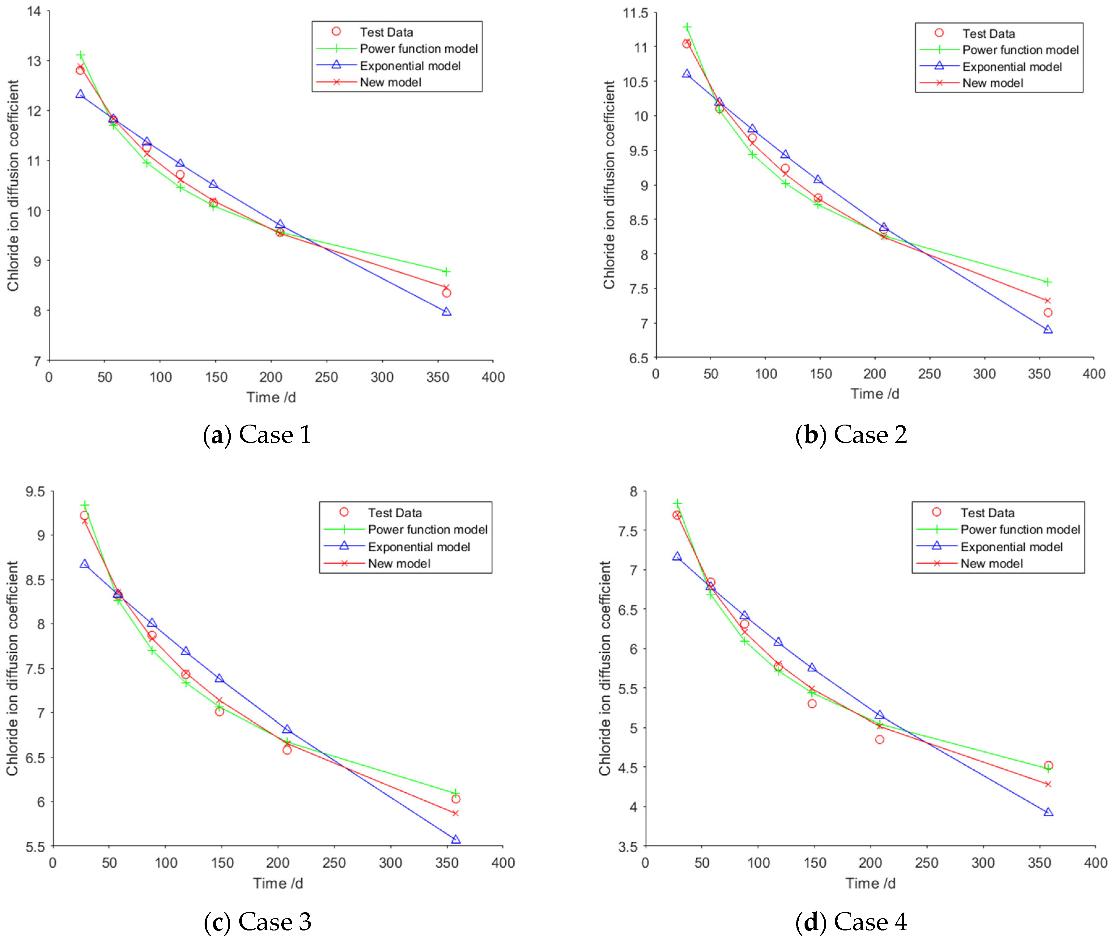
For Case 1, the fitting curves obtained using the power function model, the exponential model, and the new model are illustrated in Figure 1a. The specific fitting equations for the power function model, the exponential model, and the new model are presented in Equations (15), (16), and (17), respectively.

$$D_t=22.1639{({\displaystyle \frac{1}{t}})}^{0.1575}$$

(15)

$$D_t=12.7688e^{-0.0013t}$$

(16)

$$D_t={\displaystyle \frac{1}{0.003\sqrt{t}+0.0619}}$$

(17)

For Case 2, the fitting curves obtained using the power function model, the exponential model, and the new model are illustrated in Figure 1b. The specific fitting equations corresponding to the three models are as follows:

$$D_t=18.9424{({\displaystyle \frac{1}{t}})}^{0.1555}$$

(18)

$$D_t=10.992e^{-0.0013t}$$

(19)

$$D_t={\displaystyle \frac{1}{0.0034\sqrt{t}+0.0722}}$$

(20)

For Case 3, the fitting curves obtained using the power function model, the exponential model, and the new model are illustrated in Figure 1c. The specific fitting equations corresponding to the three models are as follows:

$$D_t=16.3157{({\displaystyle \frac{1}{t}})}^{0.1676}$$

(21)

$$D_t=9.0017e^{-0.0013t}$$

(22)

$$D_t={\displaystyle \frac{1}{0.0045\sqrt{t}+0.0855}}$$

(23)

For Case 4, the fitting curves obtained using the power function model, the exponential model, and the new model are illustrated in Figure 1d. The specific fitting equations corresponding to the three models are as follows:

$$D_t=16.2958{({\displaystyle \frac{1}{t}})}^{0.2197}$$

(24)

$$D_t=7.532e^{-0.0018t}$$

(25)

$$D_t={\displaystyle \frac{1}{0.0076\sqrt{t}+0.0897}}$$

(26)

Table 3. The mean values of fitting errors, standard deviations, and the coefficient of determination of Cases 1–4.

Case	Index	Power Function Model	Exponential Model	New Model
Case 1	Mean value of fitting error $\overline{\delta }$	0.2123	0.2476	0.0731
	Standard deviation $\sigma$	0.1571	0.1672	0.0432
	Coefficient of determination ($R^2$)	0.9644	0.9543	0.9963
Case 2	Mean value of fitting error $\overline{\delta }$	0.1937	0.1975	0.0827
	Standard deviation $\sigma$	0.1379	0.1358	0.0498
	Coefficient of determination ($R^2$)	0.9603	0.9596	0.9934
Case 3	Mean value of fitting error $\overline{\delta }$	0.0908	0.2861	0.0740
	Standard deviation $\sigma$	0.0398	0.1889	0.0537
	Coefficient of determination ($R^2$)	0.9904	0.8631	0.9921
Case 4	Mean value of fitting error $\overline{\delta }$	0.1362	0.3366	0.1140
	Standard deviation $\sigma$	0.0657	0.2052	0.0861
	Coefficient of determination ($R^2$)	0.9796	0.8631	0.9823

presents the mean values of fitting errors, standard deviations, and the coefficient of determination ($R^2$) of Cases 1–4. As can be seen from Table 3, for Case 1, the mean value and standard deviation of the fitting errors for the new model are both smaller than those of the other two models, while its coefficient of determination is higher than that of the other two models. The mean error value of the new model is approximately 34% of that of the power function model and about 30% of that of the exponential model. These results indicate that the fitting accuracy of the new model surpasses that of the two existing models. For Case 2, the mean error value of the new model is approximately 43% of that of the power function model and about 42% of that of the exponential model. For Cases 3 and 4, the mean values of the fitting errors for the new model are both smaller than those of the other two models, and their coefficients of determination are both higher. Although the standard deviation of the new model is slightly larger than that of the power function model, overall, the new model still exhibits the highest fitting accuracy.

Reference [30] presents the test results for chloride ion diffusion coefficients for four series of C45 concrete specimens with dimensions of 100 mm × 100 mm × 100 mm (referred to as Case 5 to Case 8). The mix proportions for this experiment were designed in compliance with the regulations specified in JGJ55-2011 [32] and JG/T472-2015 [33], resulting in the preparation of concrete with a strength grade of C45.

Table 4. The material mix proportions for Cases 5 to 8 (kg/m³).

Serial Number	Specimen Number	Steel Fiber Volume Fraction/%	Water-Binder Ratio	Sand Ratio	Water /kg	Water-Reducing Admixture/%
Case 5	C45	0	0.41	0.39	175	0.60
Case 6	CF45-0.5	0.5	0.41	0.39	175	0.60
Case 7	CF45-1.0	1.0	0.41	0.39	175	0.60
Case 8	CF45-1.5	1.5	0.41	0.39	175	0.60

presents the specific data for the mix proportions used in these four sets of experiments. In Table 4, “C” stands for the reference plain concrete, while “CF” represents the series of steel fiber-reinforced concrete. As can be seen from Table 4 these test specimens adopted four different steel fiber dosages of 0%, 0.5%, 1.0%, and 1.5%, respectively. Incorporating steel fibers into concrete can effectively restrain the development of internal cracks in the concrete and prevent the formation of chloride ion transport pathways, thereby reducing the impact of chloride ions on the mechanical properties of the concrete. The specimens were poured under standard conditions and then transferred to a standard curing room with a temperature of 20 °C and a relative humidity exceeding 95% for curing until they reached 28 days of age. Subsequently, the chloride ion diffusion coefficient of the steel fiber-reinforced concrete was measured at dry–wet cycle erosion ages of 30 days, 60 days, 90 days, and 120 days respectively.

Table 5. The chloride ion diffusion coefficients for Cases 5 to 8 (10⁻⁸ cm²/s).

Age	30 d	60 d	90 d	120 d
Case 5	9.71	3.89	3.42	2.25
Case 6	3.80	1.98	1.98	1.57
Case 7	4.12	2.69	2.15	1.85
Case 8	4.29	2.32	1.91	1.66

displays the chloride ion diffusion coefficient at each time point. As can be seen from Table 5, when the steel fiber content increases from 0% to 1.5%, the chloride ion diffusion coefficient first decreases and then increases, reaching its minimum value at a steel fiber content of 0.5%.

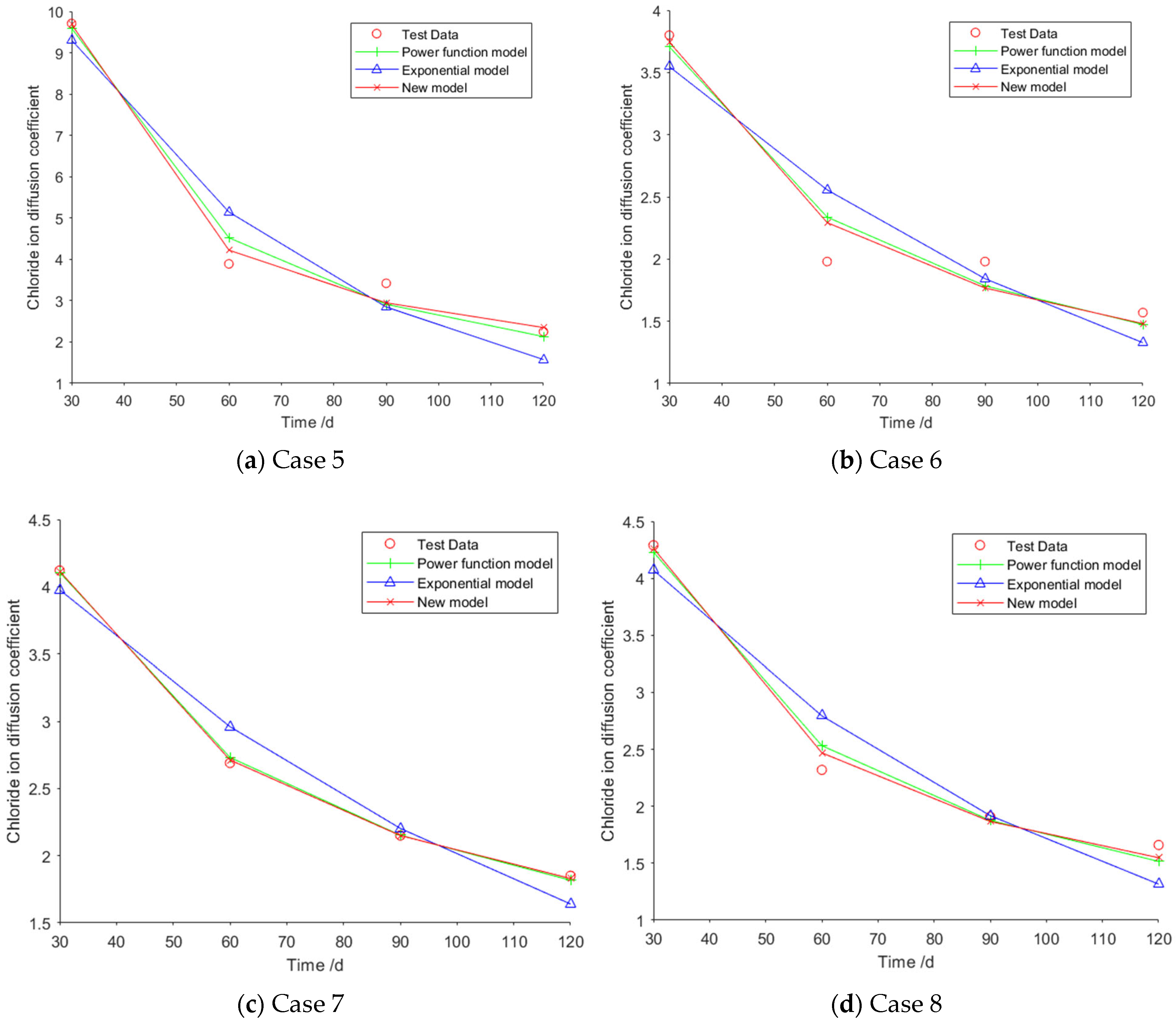
For Case 5, the fitting curves obtained using the power function model, the exponential model, and the new model are illustrated in Figure 2a. The specific fitting equations corresponding to the three models are as follows:

$$D_t=384.6845{({\displaystyle \frac{1}{t}})}^{1.0853}$$

(27)

$$D_t=16.8279e^{-0.0197t}$$

(28)

$$D_t={\displaystyle \frac{1}{0.0589\sqrt{t}-0.2192}}$$

(29)

For Case 6, the fitting curves obtained using the power function model, the exponential model, and the new model are illustrated in Figure 2b. The specific fitting equations corresponding to the three models are as follows:

$$D_t=35.6186{({\displaystyle \frac{1}{t}})}^{0.6653}$$

(30)

$$D_t=4.9218e^{-0.0109t}$$

(31)

$$D_t={\displaystyle \frac{1}{0.0745\sqrt{t}-0.141}}$$

(32)

For Case 7, the fitting curves obtained using the power function model, the exponential model, and the new model are illustrated in Figure 2c. The specific fitting equations corresponding to the three models are as follows:

$$D_t=30.3449{({\displaystyle \frac{1}{t}})}^{0.5881}$$

(33)

$$D_t=5.3418e^{-0.0098t}$$

(34)

$$D_t={\displaystyle \frac{1}{0.0554\sqrt{t}-0.0603}}$$

(35)

For Case 8, the fitting curves obtained using the power function model, the exponential model, and the new model are illustrated in Figure 2d. The specific fitting equations corresponding to the three models are as follows:

$$D_t=52.4135{({\displaystyle \frac{1}{t}})}^{0.7401}$$

(36)

$$D_t=5.9323e^{-0.0125t}$$

(37)

$$D_t={\displaystyle \frac{1}{0.0751\sqrt{t}-0.1767}}$$

(38)

Table 6. The mean values of the fitting errors, standard deviations, and coefficient of determination of Cases 5–8.

Case	Index	Power Function Model	Exponential Model	New Model
Case 5	Mean value of fitting error $\overline{\delta }$	0.3439	0.7278	0.2325
	Standard deviation $\sigma$	0.2656	0.3695	0.2069
	Coefficient of determination ($R^2$)	0.9795	0.9242	0.9897
Case 6	Mean value of fitting error $\overline{\delta }$	0.1855	0.3023	0.1676
	Standard deviation $\sigma$	0.1241	0.1898	0.1180
	Coefficient of determination ($R^2$)	0.9384	0.8412	0.9483
Case 7	Mean value of fitting error $\overline{\delta }$	0.0226	0.1692	0.0120
	Standard deviation $\sigma$	0.0179	0.0929	0.0108
	Coefficient of determination ($R^2$)	0.9990	0.9538	0.9997
Case 8	Mean value of fitting error $\overline{\delta }$	0.1127	0.2611	0.0829
	Standard deviation $\sigma$	0.0812	0.1985	0.0576
	Coefficient of determination ($R^2$)	0.9835	0.9087	0.9913

presents the mean values of the fitting errors, standard deviations, and coefficient of determination ($R^2$) of Cases 5–8. As can be seen from Table 6, the mean value and standard deviation of the fitting errors for the new model are both smaller than those of the other two models, while its coefficient of determination is higher. This indicates that the new model is the optimal predictive model for chloride ion diffusion coefficients across Cases 5 to 8.

Reference [31] employed a high volume of mineral admixtures and a relatively low water–binder ratio, with one of the experimental objectives being to investigate the effects of the water–binder ratio and the amount of mineral admixtures on the chloride ion penetration resistance of high-performance concrete resistant to chloride salts. Three series of concrete specimens with water–binder ratios of 0.3, 0.4, and 0.5 (referred to as Case 9 to Case 11) were fabricated, each with dimensions of 100 mm × 100 mm × 100 mm.

Table 7. The material mix proportions for Cases 9 to 11 (kg/m³).

Mix Ratio Number	Composition of Gelling Materials (%)				Total Gel Content	Sand	Gravel	Water	Water-Reducing Admixture
	Cement	Fly Ash	Slag	Silica Fume
Case 9	40	15	40	5	520	770	1030	152	5.2
Case 10	40	15	45	0	420	770	1030	166	2.1
Case 11	75	25	0	0	370	770	1030	174	1.7

provides the specific data on the material composition of the concrete. The slump of these specimens was controlled within the range of 180–220 mm, and the conventional curing procedure was adhered to throughout the experiment.

Table 8. The chloride ion diffusion coefficients for Cases 9 to 11 (10⁻⁸ cm²/s).

Age	28 d	56 d	90 d	180 d	365 d	730 d	1095 d	1460 d	1825 d
Case 9	1.22	1.16	1.00	0.74	0.48	0.38	0.29	0.27	0.27
Case 10	6.37	5.19	4.06	2.94	1.78	1.45	1.19	1.25	1.18
Case 11	15.33	12.31	9.16	7.54	4.60	3.36	2.67	2.02	1.92

presents the chloride ion diffusion coefficients recorded at each age. As can be seen from Table 8, the chloride ion diffusion coefficient increases with the rise in the water–binder ratio. Additionally, the chloride ion diffusion coefficient decreases as the concrete age increases, but the rate of decrease gradually slows down and approaches a stable value after a relatively long duration.

For Case 9, the fitting curves obtained using the power function model, the exponential model, and the new model are illustrated in Figure 3a. The specific fitting equations corresponding to the three models are as follows:

$$D_t=0.5278{({\displaystyle \frac{1}{t}})}^{0.3666}$$

(39)

$$D_t=1.1503e^{-0.5298t}$$

(40)

$$D_t={\displaystyle \frac{1}{1.4898\sqrt{t}+0.3506}}$$

(41)

For Case 10, the fitting curves obtained using the power function model, the exponential model, and the new model are illustrated in Figure 3b. The specific fitting equations corresponding to the three models are as follows:

$$D_t=2.1202{({\displaystyle \frac{1}{t}})}^{0.4421}$$

(42)

$$D_t=5.8025e^{-0.9047t}$$

(43)

$$D_t={\displaystyle \frac{1}{0.4367\sqrt{t}+0.0325}}$$

(44)

For Case 11, the fitting curves obtained using the power function model, the exponential model, and the new model are illustrated in Figure 3c. The specific fitting equations corresponding to the three models are as follows:

$$D_t=4.8274{({\displaystyle \frac{1}{t}})}^{0.465}$$

(45)

$$D_t=13.9338e^{-0.9236t}$$

(46)

$$D_t={\displaystyle \frac{1}{0.1936\sqrt{t}+0.0101}}$$

(47)

Table 9. The mean values of fitting errors, standard deviations, and the coefficient of determination of Cases 9–11.

Case	Index	Power Function Model	Exponential Model	New Model
Case 9	Mean value of fitting error $\overline{\delta }$	0.0695	0.1069	0.0509
	Standard deviation $\sigma$	0.0400	0.0681	0.0321
	Coefficient of determination ($R^2$)	0.9545	0.8868	0.9745
Case 10	Mean value of fitting error $\overline{\delta }$	0.1686	0.7262	0.1469
	Standard deviation $\sigma$	0.1042	0.3152	0.1092
	Coefficient of determination ($R^2$)	0.9889	0.8186	0.9905
Case 11	Mean value of fitting error $\overline{\delta }$	0.4131	1.4604	0.3852
	Standard deviation $\sigma$	0.2694	0.6356	0.1892
	Coefficient of determination ($R^2$)	0.9888	0.8814	0.9914

presents the mean values of the fitting errors, standard deviations, and coefficient of determination ($R^2$) of Cases 9–11. As shown in Table 9, for Cases 9 to 11, the mean values of the fitting errors for the new model are all lower than those of the power function model and the exponential model, while its coefficients of determination are all higher. In terms of the standard deviation of the errors, only in Case 10 is the standard deviation of the new model slightly larger than that of the power function model; in the other cases, the standard deviations of the new model are all lower than those of the other two models. Integrating the fitting results from the aforementioned 11 sets of experimental data, compared with the power function model and the exponential model, the new model exhibits the lowest mean fitting error and the highest coefficient of determination (R²) across all scenarios. In the vast majority of cases, the standard deviation of the new model is lower than that of the other two models. These results indicate that the new model has a higher fitting accuracy than the other two models. Since the new model has the smallest mean prediction error and its predicted values are closer to the experimental values, it is demonstrated that the new model’s function can more accurately describe the temporal variation pattern of chloride ion diffusion coefficients. Therefore, the new model likely reflects the fundamental law governing the temporal variation of chloride ion diffusion coefficients.

It is observed that for certain cases, the fitting accuracies of the new model and the power function model are relatively close. However, when the time $t$ is significantly large, there can be substantial differences in the predicted chloride ion diffusion coefficient values between these two models. Without loss of generality,

Table 10. The chloride ion diffusion coefficients predicted by the three models for Cases 1–4 on the 600th day.

Case	Power Function Model	Exponential Model	New Model
Case 1	8.0948	5.7932	7.4185 (9.1%) *
Case 2	7.0057	5.0297	6.4257 (9.0%)
Case 3	5.5862	4.0243	5.1140 (9.2%)
Case 4	3.9980	2.5174	3.6223 (10.4%)

* The data within the parentheses represent the relative error between the predicted values of the new model and those of the power function model.

presents the chloride ion diffusion coefficients predicted by the three models on the 600th day for Cases 1 to 4.

Table 11. The chloride ion diffusion coefficients predicted by the three models for Cases 5–8 on the 150th day.

Case	Power Function Model	Exponential Model	New Model
Case 5	1.6725	0.8702	1.9928 (16.1%) *
Case 6	1.2706	0.9568	1.2962 (2.0%)
Case 7	1.5936	1.2208	1.6180 (1.5%)
Case 8	1.2854	0.9035	1.3460 (4.5%)

* The data within the parentheses represent the relative error between the predicted values of the new model and those of the power function model.

provides the predicted chloride ion diffusion coefficients by the three models on the 150th day for Cases 5 to 8.

Table 12. The chloride ion diffusion coefficients predicted by the three models for Cases 9–11 on the 3650th day.

Case	Power Function Model	Exponential Model	New Model
Case 9	0.2269	0.0058	0.1976 (14.8%) *
Case 10	0.7661	0.0006	0.7075 (8.3%)
Case 11	1.6548	0.0014	1.6066 (3.0%)

* The data within the parentheses represent the relative error between the predicted values of the new model and those of the power function model.

offers the predicted chloride ion diffusion coefficients by the three models on the 3650th day for Cases 9 to 11.

From Table 10, it can be seen that for Cases 1 to 4, the errors between the predicted values of the new model and those of the power function model all exceed 5%, with some exceeding 10%. From Table 11, the error between the predicted values of the new model and the power function model for Case 5 exceeds 15%. From Table 12, the error between the predicted values of the new model and the power function model for Case 9 approaches 15%, while for Case 10, the error between the predicted values of the two models exceeds 5%. These data indicate that when the time $t$ is significantly large, there can be considerable differences in the predicted chloride ion diffusion coefficient values between the new model and the power function model. Therefore, the new model developed in this paper still holds significant reference value for predicting the chloride ion diffusion coefficient of concrete structures in engineering practice. Its predictions, along with those of the power function model, could potentially serve as upper and lower bounds for assessing the durability of concrete structures, thereby enabling more scientific decisions regarding subsequent structural maintenance.

5. Application in the Prediction of Remaining Service Lives of Concrete Structures

Based on the aforementioned formula for chloride ion diffusion coefficient, the estimation formula [34] for the chloride ion concentration at a depth of $h$ from the concrete surface at time $t$ is as follows:

$$C_{h,t}=C_s[1-erf({\displaystyle \frac{h}{2\sqrt{D_{t}t}}})]$$

(48)

where $C_{h,t}$ represents the chloride ion concentration at a depth of $h$ from the concrete surface at time $t$, $C_s$ denotes the chloride ion concentration at the concrete surface, and $erf(\cdot )$ stands for the error function [34,35]. Substituting Equation (3) into (48) yields the estimation formula for chloride ion concentration based on the model proposed in this work as follows:

$$C_{h,t}=C_s[1-erf({\displaystyle \frac{h}{2\sqrt{\frac{t}{a\sqrt{t}+b}}}})]$$

(49)

It is generally believed that when the chloride ion concentration within the thickness of the concrete cover reaches the corrosion-inducing concentration threshold, the concrete structure has reached the end of its service life. Therefore, given the thickness $h$ of the concrete cover and the corrosion-inducing concentration threshold, one can back-calculate the time $t$ based on Equation (49). This time $t$ represents the total service life of the concrete structure. By subtracting the time that has already elapsed since the structure was put into service, the remaining service life can be obtained.

Next, the concrete structure of a coastal wharf [35] will be used as an example to specifically elaborate on the process of estimating its remaining service life. The concrete strength grade of this wharf structure is C40, with a concrete cover thickness of 65 mm, and it has been in service for 12.83 years. The chloride ion diffusion coefficients at four different ages have been tested and are shown in

Table 13. Chloride ion diffusion coefficients of the wharf structure at four different ages.

Age/yr	5	5.17	9	12.83
$D_t$	47.22	45.68	39.15	28.08

.

By performing curve fitting using the proposed model based on the data in Table 13, one has

$$D_t={\displaystyle \frac{1}{0.0086\sqrt{t}+0.0019}}$$

(50)

It can be seen from Equation (50) that $a=0.0086$ and $b=0.0019$. Based on engineering experience, the corrosion-inducing chloride ion concentration threshold can be taken as 0.08. Based on measurements, the chloride ion concentration on the concrete surface is determined to be 0.61. From Equation (49), when $C_{h,t}$ = 0.08, $C_s$ = 0.61 and $h$ = 65 mm, the time $t$ can be back-calculated to be approximately 67.4 years. By subtracting the 12.83 years that the structure has already been in service, we can determine that the remaining service life is 54.57 years.

6. Conclusions

This paper introduces a new predictive model for analyzing how the chloride ion diffusion coefficient in concrete changes over time. The proposed model offers a more straightforward physical interpretation compared to existing ones, as it demonstrates a linear relationship between the reciprocal of the chloride ion diffusion coefficient and the square root of time. Using 11 sets of experimental data, the proposed time-varying model for the chloride ion diffusion coefficient was compared with existing power function models and exponential models. A comparison of the computational results reveals that, for all scenarios, the new model exhibits a lower mean fitting error than both the power function model and the exponential model, while achieving the highest coefficient of determination. In terms of the standard deviation of the errors, the new model’s fitting standard deviation is lower than those of the other two models in the vast majority of scenarios. Overall, the new model consistently demonstrates the lowest mean fitting error and the highest coefficient of determination across all conditions, indicating its superior fitting accuracy. This also suggests that the new model may capture the fundamental physical law governing the temporal variation of chloride ion diffusion coefficients within concrete. Whether for theoretical research on concrete durability or engineering applications, the time-varying model of chloride ion diffusion coefficients proposed in this paper holds significant reference value. The potential areas for further research primarily encompass two aspects. The first is to employ a greater volume of experimental data, particularly long-term test data from actual engineering projects, to further validate and enhance the time-varying model of the chloride ion diffusion coefficient proposed in this paper. The second aspect involves integrating the proposed model with neural network models to more effectively overcome the adverse impacts of measurement errors present in the experimental data.