Shear Force–Displacement Curve of a Steel Shear Wall Considering Compression

Abstract

The shear strength of a steel shear wall (SSW) is typically governed by the yield strength of the steel. However, changes in mechanical properties beyond yielding—particularly those related to steel hardening and the effects of gravity loads—are not yet fully understood. These factors are critical for accurately assessing the shear capacity of SSWs during seismic events. In the current study, a method to calculate the shear force–displacement curve of a steel shear wall while considering the compression effect is presented, which incorporates both steel hardening and gravity effects. The analysis derives strains in tensile strips undergoing shear deformation using a strip model. Corresponding stresses are then determined using the stress–strain relationships obtained from tensile tests of the steel. Furthermore, the vertical stress induced by gravity loads is modeled using a three-segment distribution proposed before. For each tensile strip, the tension field stress is calculated by accounting for reductions due to vertical stress and the influence of steel hardening through the von Mises yield criterion. This approach enables the development of a shear force–displacement curve, which is subsequently validated against results from an experimentally verified finite element model. The findings demonstrate that the pushover curves predicted by this method closely align with those obtained from finite element analysis. Notably, the results indicate that the shear strength provided by the CAN/CSA-S16-01 equation may be overestimated by approximately 4%, 9%, and 18% when the vertical compression stresses are 50, 100, and 150 MPa for a wall with a slenderness of 150, respectively.

1. Introduction

Steel shear walls (SSWs) have emerged as a prominent lateral force resistance system for tall structures over the past three decades. Originally, SSWs incorporated stiffeners to mitigate buckling, with shear strength evaluated based on the onset of buckling. However, a groundbreaking finding by Thorburn et al. revealed that SSWs retain the capacity to resist shear forces post-buckling, thus paving the way for innovative research avenues [1]. Early investigations primarily centered on cyclic loading tests [2,3,4,5], while recent studies conducted by Han et al. [6], Wang et al. [7], and others have shifted focus towards the design and exploration of advanced SSW configurations, underscoring the evolving understanding and application of this structural system [8,9,10,11,12,13,14,15,16,17,18].

Previous research on steel shear walls (SSWs) has primarily concentrated on determining their shear strength to satisfy practical application requirements. However, there has been insufficient attention paid to the shear strength dynamics post-steel yielding and the influence of steel hardening, often relegating this to merely a safety margin. In the context of strong earthquakes, SSWs experience a plastic stage where shear strength can substantially increase due to the hardening effect, making it critical to include this factor in seismic performance evaluations. Furthermore, existing studies have largely overlooked the effects of gravity loads on SSW seismic performance, despite their bearing of such loads during construction. For example, in the Tianjin World Financial Center project, the infilled steel walls were installed synchronously with the boundary steel frames to speed up the construction process; surely, the infilled steel walls will resist gravity together with the boundary frames from the unfinished levels.

This study aims to investigate the hardening behavior of steel and the influence of gravity loads on the seismic performance of steel plate shear walls (SPSWs). A method to calculate the shear force–displacement curve of a steel shear wall while considering the compression effect is presented to accurately characterize the shear response of SPSWs, requiring the determination of tensile strip strains under specified deformations and the derivation of corresponding stresses from the steel’s stress–strain relationship obtained through tensile testing. The methodology incorporates a vertical stress distribution proposed by the authors to evaluate the detrimental effects of gravity loads. By integrating vertical stresses and the steel hardening effect, the tension field stresses within the tensile strips are derived using the von Mises yield criterion. The proposed approach is validated through a finite element model (FEM), followed by parametric studies conducted to assess its efficacy.

2. Shear Capacity Model

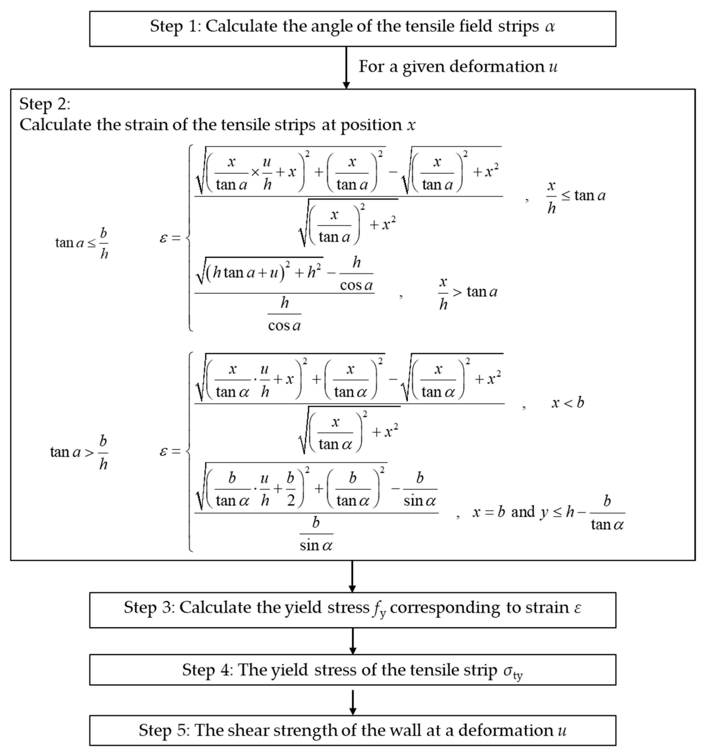
2.1. Strain of the Tensile Strips

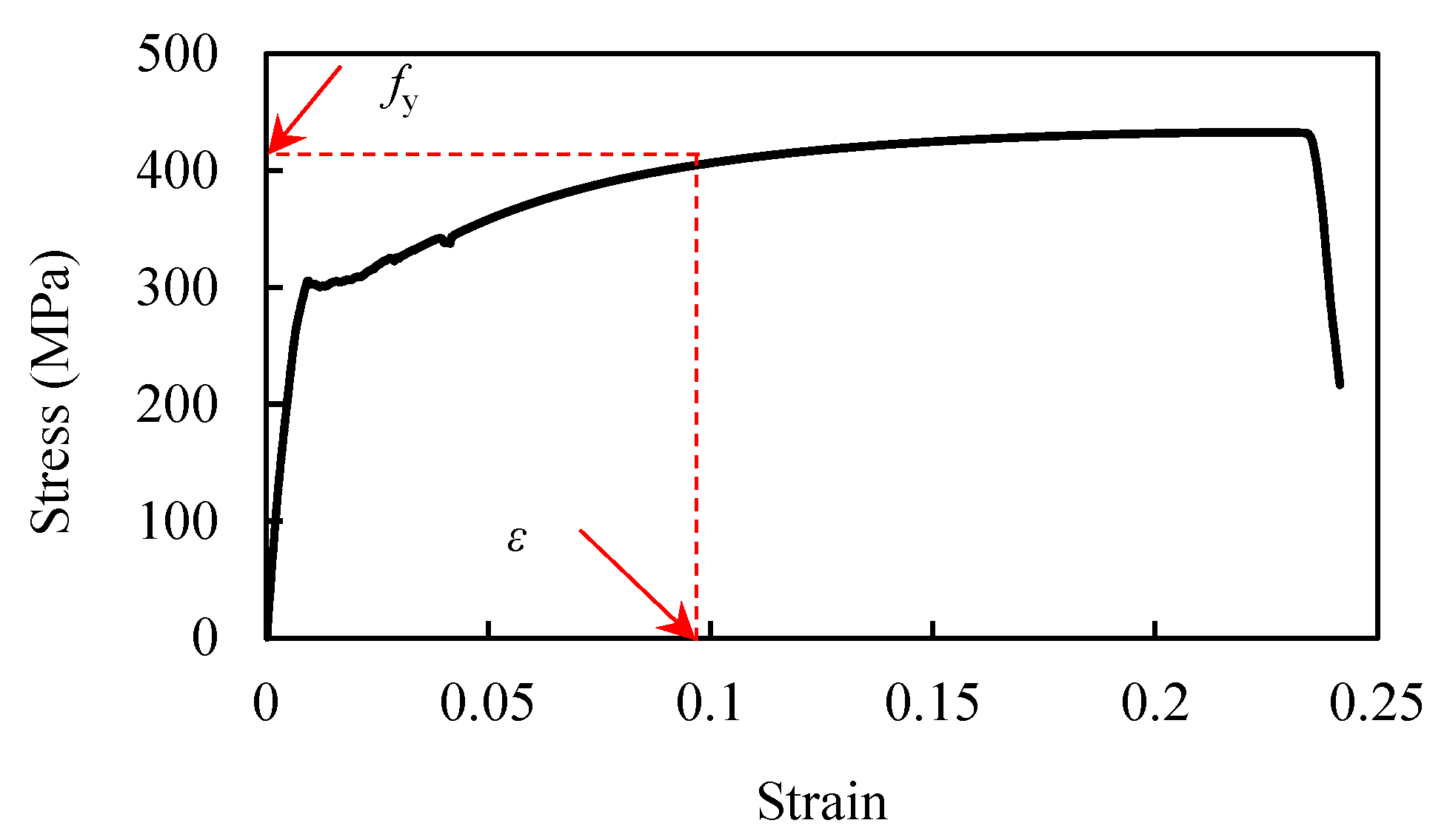
In this study, the shear wall is represented as a sequence of strips that are linked to a boundary frame through pinned connections, oriented at an angle θ. The angle of the tensile field relative to the vertical axis [18] is defined using

$$\alpha ={\displaystyle \frac{\pi }{2}}-{\tan }^{-1}\sqrt[4]{\left(1+{\displaystyle \frac{tb}{2A_c}}\right){\left[1+th\left({\displaystyle \frac{1}{A_{\mathrm{b}}}}+{\displaystyle \frac{h^3}{360I_{\mathrm{c}}{b}^2}}\right)\right]}^{-1}}$$

(1)

where A_c and I_c are the cross-sectional area of the column and moment of inertia of the column, respectively. A_b is the cross-sectional area of the beam. h is the wall height, and b is the wall width.

To establish the shear–deformation relationship of the wall, it is essential to correlate the strain of the tensile strip with the deformation of the wall, which can be accurately derived using the tensile strip model in conjunction with the geometric relationships illustrated in Figure 1.

If $\tan a\le {\displaystyle \frac{b}{h}}$, see Figure 1a, then the strain of the tensile strips at position x in the width direction is

$$\epsilon =\left\{\begin{array}{l}{\displaystyle \frac{\sqrt{{\left(\frac{x}{\tan a}\times \frac{u}{h}+x\right)}^2+{\left(\frac{x}{\tan a}\right)}^2}-\sqrt{{\left(\frac{x}{\tan a}\right)}^2+x^2}}{\sqrt{{\left(\frac{x}{\tan a}\right)}^2+x^2}}}\hspace{1em},\hspace{1em}{\displaystyle \frac{x}{h}}\le \tan a\\ {\displaystyle \frac{\sqrt{{\left(h\tan a+u\right)}^2+h^2}-\frac{h}{\cos a}}{\frac{h}{\cos a}}}\hspace{1em},\hspace{1em}{\displaystyle \frac{x}{h}}>\tan a\end{array}\right.$$

(2)

If $\tan a>{\displaystyle \frac{b}{h}}$, see Figure 1b, then the strain of the tensile strips at position y in the height direction is

$$\epsilon =\left\{\begin{array}{l}{\displaystyle \frac{\sqrt{{\left(\frac{x}{\tan \alpha }·\frac{u}{h}+x\right)}^2+{\left(\frac{x}{\tan \alpha }\right)}^2}-\sqrt{{\left(\frac{x}{\tan \alpha }\right)}^2+x^2}}{\sqrt{{\left(\frac{x}{\tan \alpha }\right)}^2+x^2}}}\hspace{1em},\hspace{1em}x<b\\ {\displaystyle \frac{\sqrt{{\left(\frac{b}{\tan \alpha }·\frac{u}{h}+\frac{b}{2}\right)}^2+{\left(\frac{b}{\tan \alpha }\right)}^2}-\frac{b}{\sin \alpha }}{\frac{b}{\sin \alpha }}}\hspace{1em},\hspace{1em}x=b \mathrm{and} y\le h-{\displaystyle \frac{b}{\tan \alpha }}\end{array}\right.$$

(3)

u is the deformation at the top of the wall. x and y, as shown in Figure 1, are the positions of the calculated strip along the horizontal and vertical directions, respectively.

2.2. Yield Stress

For a specified displacement u at the top of the SSW, the strain in the tensile strips can be accurately calculated by Equations (2) and (3). With the strain determined, the yield stress f_y can then be derived by considering the hardening effects of steel, as outlined in the associated stress–strain relationship shown in Figure 2. This procedure for obtaining the stress–strain relationship is both practical and cost-effective, facilitating the integration of material properties into structural design.

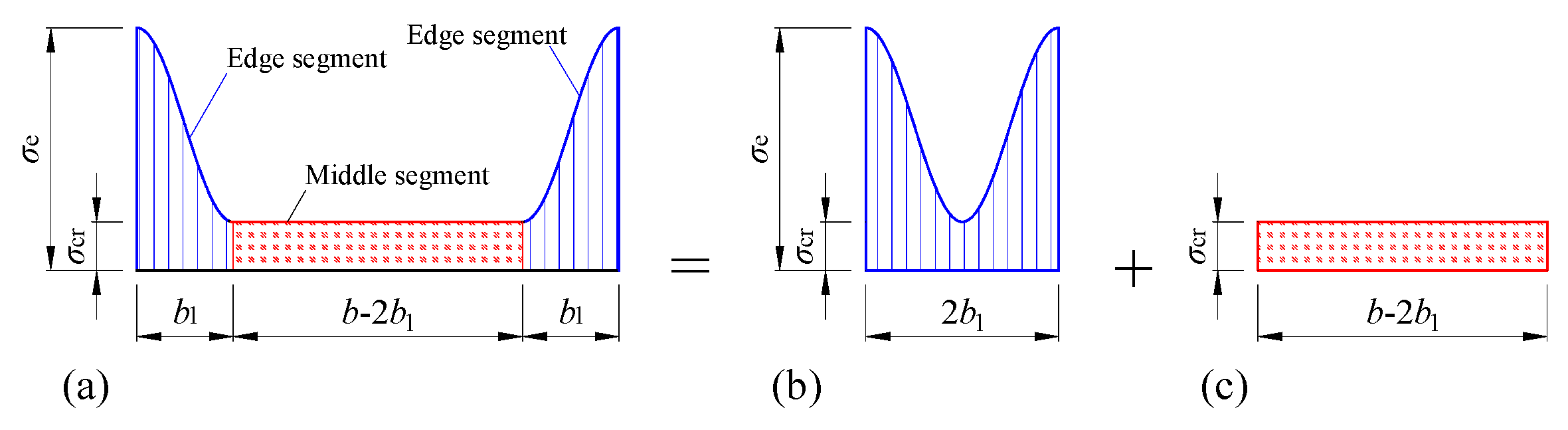
2.3. Stress Under Compression

The vertical stress is considered by the vertical stress distribution [19,20] proposed before (see Figure 3):

$$\sigma (x)=\left\{\begin{array}{l}{\displaystyle \frac{{\sigma }_{\mathrm{e}}+{\sigma }_{\mathrm{cr}}}{2}}+{\displaystyle \frac{{\sigma }_{\mathrm{e}}-{\sigma }_{\mathrm{cr}}}{2}}\cos (\mathsf{\pi }{\displaystyle \frac{x}{b_1}}), 0\le x\le b_1\\ {\sigma }_{\mathrm{cr}}, b_1<x\le b-b_1\\ {\displaystyle \frac{{\sigma }_{\mathrm{e}}+{\sigma }_{\mathrm{cr}}}{2}}+{\displaystyle \frac{{\sigma }_{\mathrm{e}}-{\sigma }_{\mathrm{cr}}}{2}}\cos (\mathsf{\pi }{\displaystyle \frac{x-B}{b_1}}), b-b_1<x\le b\end{array}\right.$$

(4)

where, in Equation (4), b₁ is the effective width of the SSW. σ_e is the axial stress of the boundary columns under gravity. σ_cr is the buckling stress of the infilled steel wall. x is the position along the horizontal direction of the wall.

2.4. Stress Analysis of the Wall Under Compression and Shear

The behavior of a wall under shear is characterized by two distinct stages. Initially, prior to or at the point of buckling, the stress of the wall is described by

$$\left\{\begin{array}{l}{\sigma }_{xx}=0\\ {\sigma }_{yy}=\sigma (x)\\ {\sigma }_{xy}={\tau }_{\mathrm{cr}}\end{array}\right.$$

(5)

where σ(x) represents the stress as derived from Equation (4), and τ_cr denotes the elastic shear buckling stress.

$$\left\{\begin{array}{l}{\sigma }_{xx}(x)={\sigma }_{\mathrm{ty}}(x){\sin }^2\alpha \\ {\sigma }_{yy}(x)=\sigma \left(x\right)+{\sigma }_{\mathrm{ty}}(x){\cos }^2\alpha \\ {\sigma }_{xy}(x)={\tau }_{\mathrm{cr}}+0.5{\sigma }_{\mathrm{ty}}(x)\sin 2\alpha \end{array}\right.$$

(6)

where σ_ty(x), σ_xx(x), σ_yy(x), and σ_xy(x) are the tensile, horizontal, vertical, and shear stresses at position x in the width direction and are respectively denoted as σ_ty, σ_xx, σ_yy, and σ_xy. α = π/2-θ and θ is calculated by Equation (1). The yield stress of the tensile strip, σ_ty, is determined through the methodologies outlined in references [21,22]:

$$\begin{array}{ll}{\sigma }_{\mathrm{ty}}=& -{\displaystyle \frac{1}{2}}[\sigma (x)(3{\cos }^2\alpha -1)+3{\tau }_{cr}\sin (2\alpha )]\\ & +{\displaystyle \frac{1}{2}}\sqrt{{[\sigma (x)(3{\cos }^2\alpha -1)+3{\tau }_{cr}\sin (2\alpha )]}^2-4[\sigma {\left(x\right)}^2+3{\tau }_{cr}^2-f_{\mathrm{y}}^2]}\end{array}$$

(7)

where, in Equation (7), the yield stress f_y is directly obtained from the material’s stress-strain curve at strains determined by Equations (2) or (3). The shear strength of the shear wall can be calculated by integrating the stresses along the width of the wall:

$$V_{\mathrm{p}}={\displaystyle {\int }_0^{L}t{\sigma }_{xy}}\mathrm{d}x={\displaystyle {\int }_0^{L}t{\sigma }_{\mathrm{ty}}\sin \alpha \cos \alpha }\mathrm{d}x$$

(8)

The calculation process is summarized in Figure 4. The calculation process is summarized as follows:

Step 1: The angle of the tensile field relative to the horizontal axis is calculated by Equation (1). In this step, the geometrical parameters of the steel wall are required, including the cross-sectional area of the column A_c, moment of inertia of the I_c, cross-sectional area of the beam A_b, the thickness of the wall t, the wall height h, and the wall width b.

Step 2: Under a given displacement of the wall u, the strain of the tensile strips at position x is calculated (see Figure 1). It was found that under a given displacement at the top of the wall, the tensile strain of each strip is the same. The strain of each strip can be calculated by Equations (2) or (3) depending on the span height ratio.

Step 3: Once the tensile stain of each strip has been obtained, the stress of the strip can be determined by checking the stress–strain curve obtained from the coupon test (see Figure 2). If the vertical load on the wall was not considered, then the shear force of the wall can be calculated by V_stan = 0.5 f_y t L sin(2α). Here, f_y is the stress corresponding to the calculated strain under the given displacement u.

Step 4: The vertical stress on the wall will weaken the shear strength of the wall, which was considered by the proposed three-segment distribution (see References [19,20]). Considering the vertical stress of the wall, the yield stress of the tensile strip σ_ty is smaller than that without considering the vertical load. σ_ty is calculated by Equation (7). In Equation (7), f_y is directly obtained from the material’s stress–strain curve at strains determined by Equations (2) or (3), and σ(x) is the vertical compression stress obtained by the three-segment distribution.

Step 5: Once the above yield stress of the tensile strip σ_ty is calculated, the shear force of the wall under the given displacement u can be calculated by Equation (8).

Since the displacement u is given, then the shear force–displacement curve can be determined.

3. Finite Element Analysis

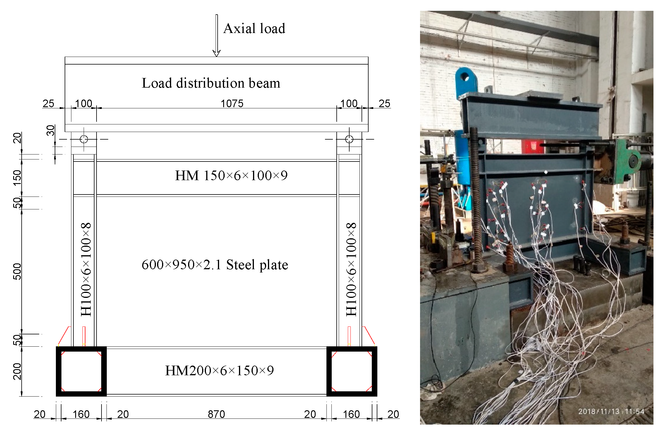
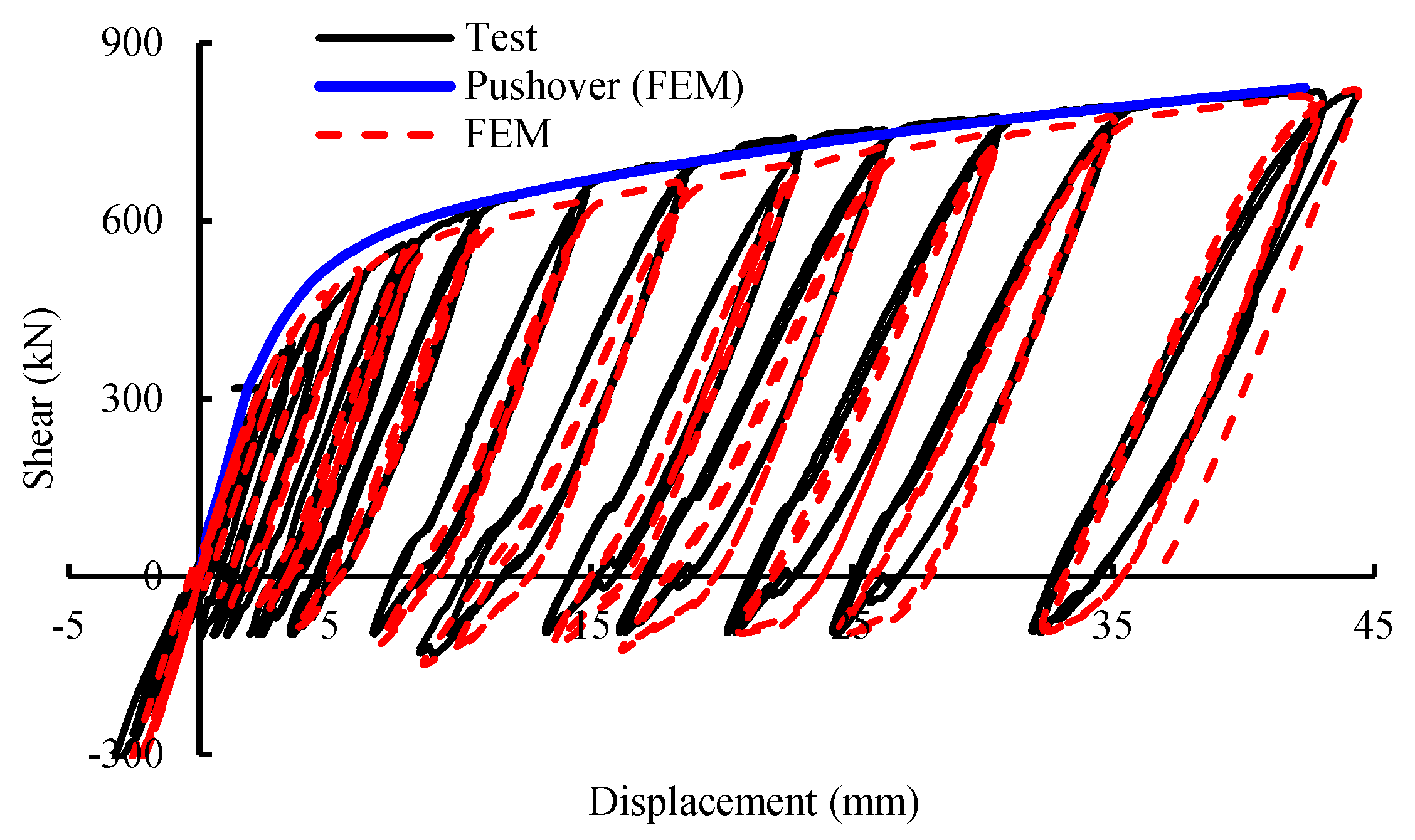
3.1. Finite Element Model and Verification

The authors completed a test on a one-storey shear wall (SSW) specimen, as shown in Figure 5, measuring 0.75 m in height and 1.10 m in width, with a wall thickness of 2.10 mm. The infill steel wall comprised Q235 steel, characterized by a yield strength of 232.1 MPa, while the boundary frame was constructed from Q390 steel, exhibiting a higher yield strength of 456.2 MPa. The boundary columns were designed as built-up sections of dimensions 100 × 100 × 6 × 8, and the top beam measured 150 × 100 × 6 × 9, all featuring rigid beam-to-column connections. An axial load of 486.2 kN was applied, generating an axial stress of approximately 100 MPa in the boundary columns. Subsequently, horizontal cyclic loading was introduced, incrementally increasing by 50 kN until the initial yield in the steel wall was observed. The loading protocol incorporated displacement-controlled loading during the push phase and force-controlled loading during the pull phase, with the maximum pull load capped at 100 kN. This approach simulated earthquake conditions, highlighting the effectiveness of the finite element method (FEM) in evaluating the wall’s performance. The deformation of the SSW was obtained by using two linear variable differential transformers (LVDTs). The mechanical properties of Q390 steel and Q235 steel are shown in Figure 6 and listed in

Table 1. Properties of steels.

Steel	t (mm)	fy (MPa)	fu (MPa)	Elongation at Break (%)
Q390	5.0/10.0	456.2	562.1	21.41
Q235	2.10	232.1	376.2	18.30

.

A refined finite element method (FEM) simulation utilizing layered shell elements was employed to assess the test conditions, with an element size of 10 mm established through sensitivity analysis. The initial wall imperfection was modeled using the first mode shape, which showed a maximum out-of-plane deformation of 1/500 of the wall height. The plastic-kinematic model was selected to simulate the property of the steel. The yield stress of different steels is shown in Table 1. After yielding, the strain hardening modulus in the stress–strain relationship is 1% of the elastic modulus E_s. The walls were fully constrained at the bottom. For the vertical and top boundaries, all the degrees of freedom were constrained except the vertical one. A load was applied at the top of the boundary columns, and pushover analysis was conducted subsequently. Results presented in Figure 7 indicate a strong correlation between the hysteresis curves from the finite element analysis and the experimental data, although the pushover analysis yielded slightly higher shear strength and stiffness values.

Figure 8 illustrates the failure shape from the finite element analysis, confirming the FEM’s effectiveness in characterizing the seismic behavior of the walls and supporting its use for the parametric analysis of SSWs.

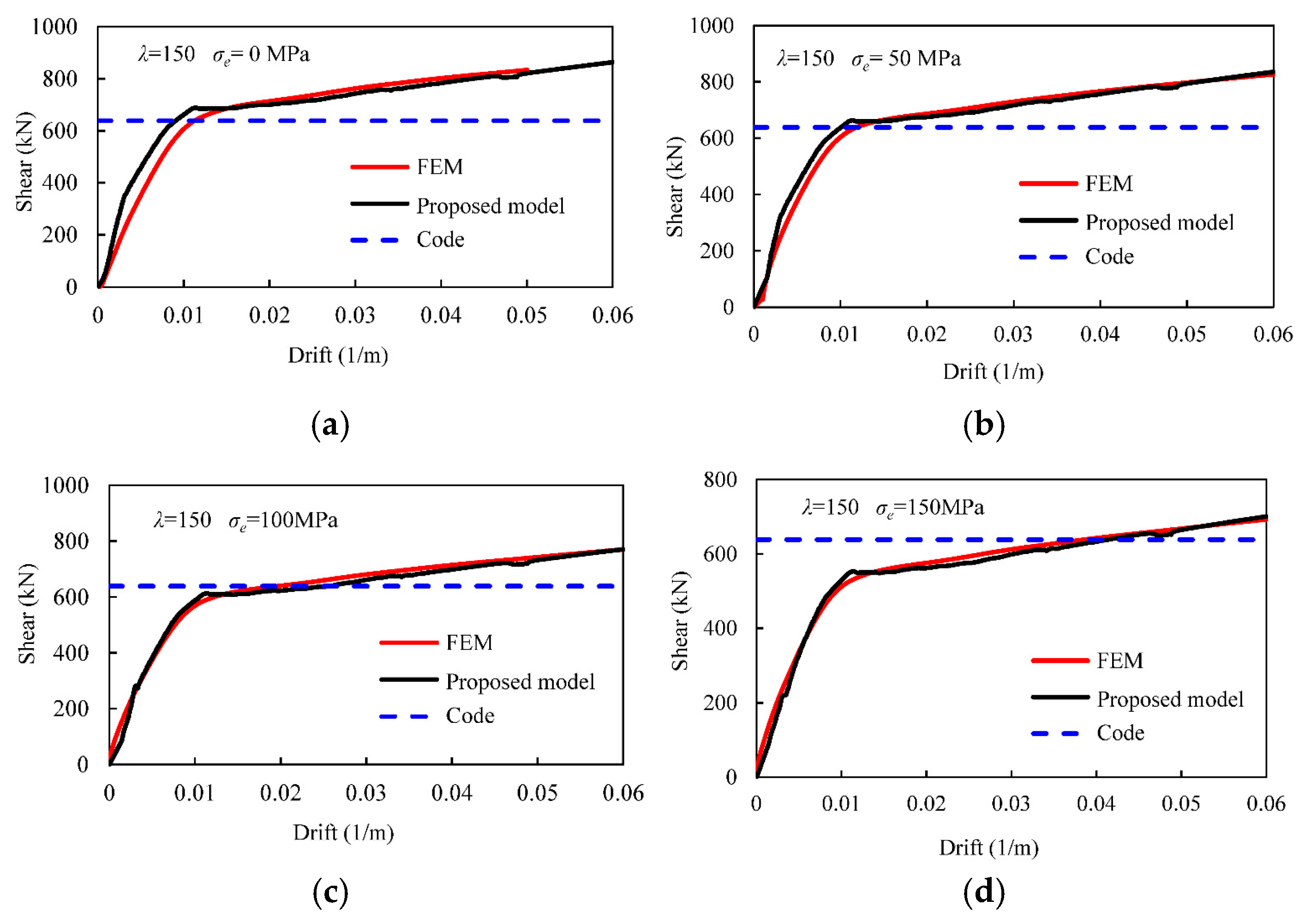
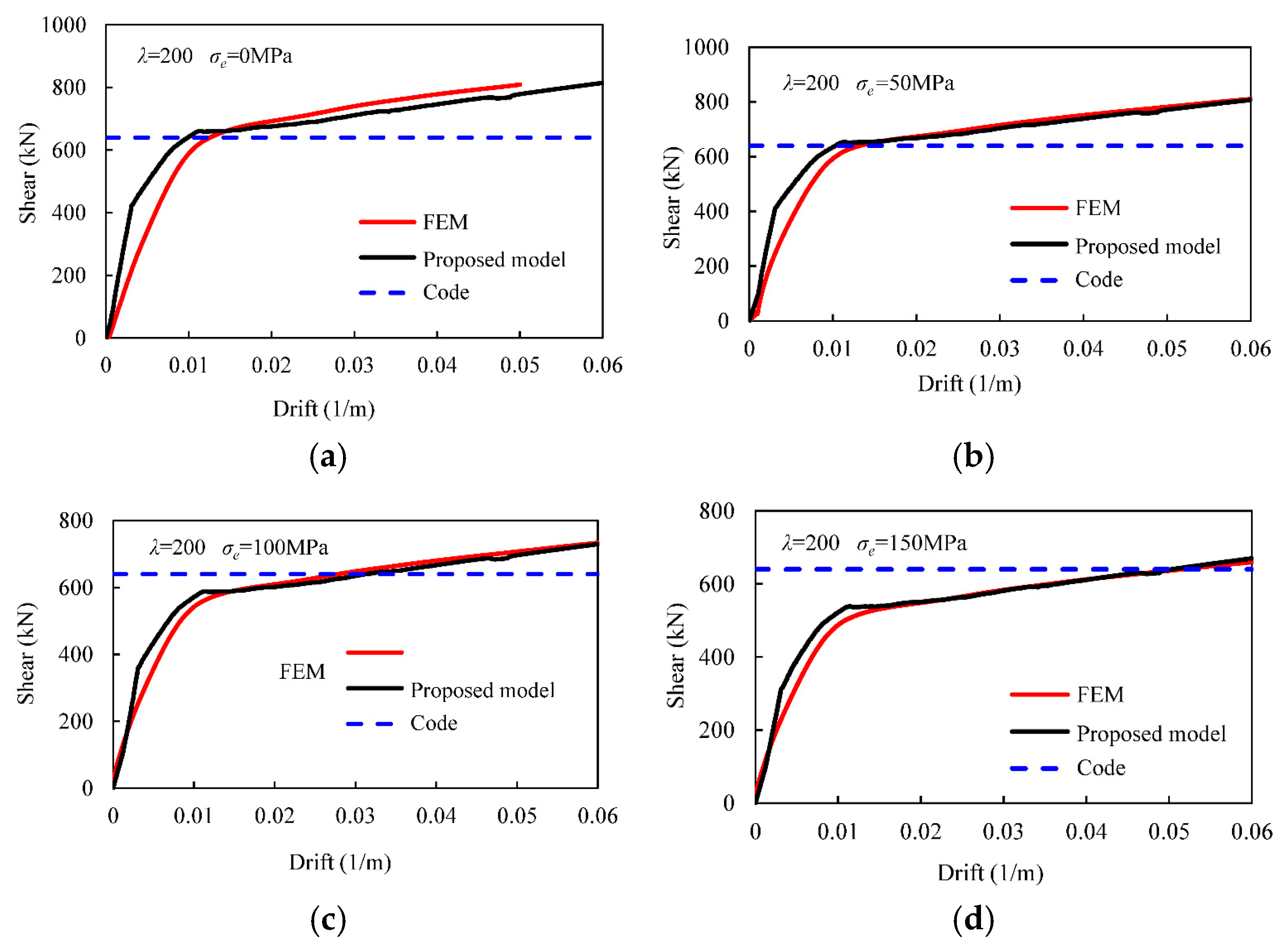
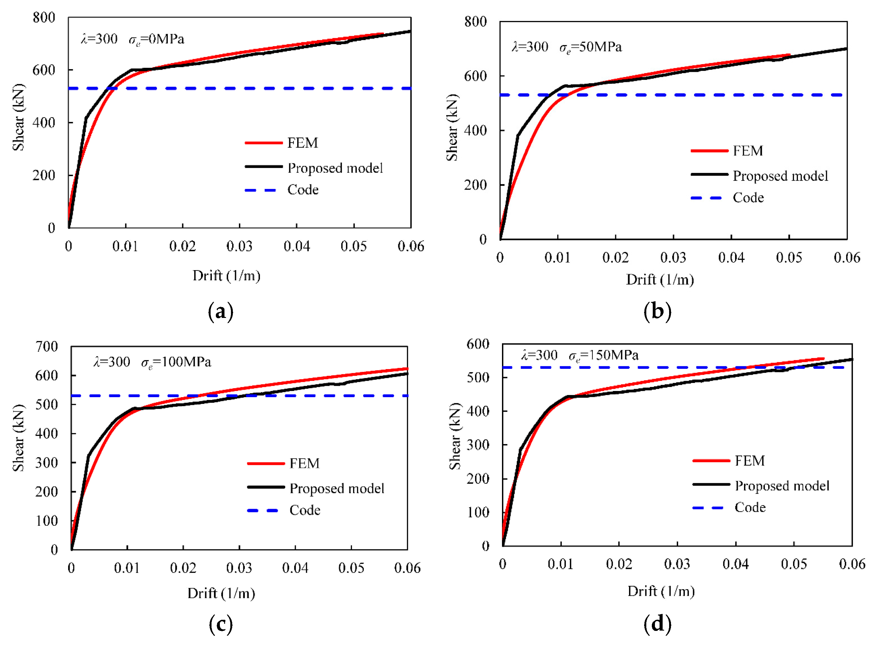
3.2. Parametric Analysis

Using the validated model, a parametric study was conducted, analyzing slenderness and vertical stress for test-equivalent walls across four axial stress levels and three wall thicknesses, resulting in slenderness values of 300, 200, and 150. In total, approximately 12 pushover analyses were performed as part of this investigation (

Table 2. Parametric analysis.

Cases	1	2	3	4	5	6	7	8	9	10	11	12
Thickness t (mm)	4	3	2	4	3	2	4	3	2	4	3	2
Axial Stress σe (MPa)	0	0	0	50	50	50	100	100	100	150	150	150

).

The capacity of the shear walls obtained from FE analyses is determined using the drift angle according to ANSI-AISC 341-05 (Seismic provisions for structural steel buildings [23]). In this specification, the capacity is defined at an inter-storey drift angle of 0.02 radians.

4. Results and Discussions

V_stan is the shear strength calculated according to the Canadian standard [24]

V_stan = 0.5 R_y f_y t L sin(2α)

(9)

where R_y is the ratio of the mean steel yield stress to the specified minimum yield stress. In this work, a ratio R_y of 1.0 is selected.

Figure 9, Figure 10 and Figure 11 illustrate a comparative analysis of shear drift relationships derived from finite element methods (FEMs), the proposed model, and the equations outlined in codes [23,24]. The findings indicate a close correlation between the analytical results of the proposed model and those generated by FEM, particularly regarding initial stiffness, yield load, yield displacement, and post-buckling bearing capacity. Additionally, the analysis reveals that increased vertical loads diminish the shear strength of SSWs. Specifically, for a height-to-thickness ratio of 150, the yield load at a 0 MPa vertical load surpasses that at higher vertical loads, demonstrating a decrease of approximately 4%, 9%, and 18% for 50, 100, and 150 MPa loads, respectively. Figure 9a, Figure 10a and Figure 11a further indicate that without considering vertical loads, the code’s predictions for shear strength are generally comparable to or slightly lower than those from the proposed model and FEM. Conversely, when accounting for vertical loads, the code tends to overestimate shear strength compared to the proposed model and FEM results. Overall, the proposed model reliably forecasts the shear strength of the SSWs, effectively incorporating the effects of steel hardening and gravity loads.

5. Conclusions

Based on the analysis conducted, a shear strength model for SSWs, incorporating the effects of steel hardening and gravity loads, has been proposed. Results obtained from numerical analysis, theoretical calculation, and code are compared and discussed. The findings show that

(1)

The proposed model offers a significant advancement in accurately predicting the true shear strength of SSWs. Notably, it is capable of generating a complete shear force–displacement curve by utilizing the stress–strain relationships obtained from the tensile testing of steel materials. Furthermore, the model facilitates the precise determination of key parameters, including initial stiffness, yield load, yield displacement, and post-buckling bearing capacity, which are crucial for understanding structural performance during and after yielding.

(2)

An important finding is the tendency for some existing code equations to overestimate the seismic performance of SSWs, particularly in cases involving heavily loaded or stocky wall configurations. For example, the CAN/CSA-S16-01 equation may be overestimated by approximately 4%, 9%, and 18% when the vertical compression stress is 50, 100, and 150 MPa for a wall with a slenderness of 150, respectively. This observation highlights the necessity for engineers to exercise caution when employing code equations in situations not fully addressed by current standard provisions.

(3)

It is essential to recognize the limitations of the proposed model. Specifically, its application is currently restricted to pushover analysis, thereby necessitating further research to thoroughly assess its validity under cyclic loading conditions typical of seismic events. Future investigations aimed at evaluating the cyclic behavior of SSWs will be vital in establishing the comprehensive practicality and reliability of the proposed model for seismic design applications.

References

1. Thorburn, L.J.; Kulak, G.L.; Montgomery, C.J. Analysis of Steel Plate Shear Walls; Report No. 107; Department of Civil Engineering, University of Alberta: Edmonton, AB, Canada, 1983. [Google Scholar]
2. Driver, R.G.; Kulak, G.L.; Kennedy, D.J.L.; Elwi, A.E. Cyclic test of a four-storey steel plate shear wall. ASCE J. Struct. Eng. 1998, 124, 112–120. [Google Scholar] [CrossRef]
3. Behbahanifard, M.R. Cyclic Behavior of Unstiffened Steel Plate Shear Walls. Ph.D. Dissertation, Department of Civil Engineering, University of Alberta, Edmonton, AB, Canada, 2003. [Google Scholar]
4. Moghimi, H.; Driver, R.G. Economical steel plate shear walls for low-seismic regions. ASCE J. Struct. Eng. 2013, 139, 379–388. [Google Scholar] [CrossRef]
5. Qu, B.; Bruneau, M.; Lin, C.H.; Tsai, K.C. Testing of full-scale two-storey steel plate shear wall with reduced beam section connections and composite floors. ASCE J. Struct. Eng. 2008, 134, 364–373. [Google Scholar] [CrossRef]
6. Han, Q.; Zhang, Y.; Wang, D.; Sakata, H. Seismic behavior of buckling-restrained steel plate shear wall with assembled multi-RC panels. J. Constr. Steel Res. 2019, 157, 397–413. [Google Scholar] [CrossRef]
7. Wang, W.; Ren, Y.; Lu, Z.; Song, J.; Han, B.; Zhou, Y. Experimental study of the hysteretic behaviour of corrugated steel plate shear walls and steel plate reinforced concrete composite shear walls. J. Constr. Steel Res. 2019, 160, 136–152. [Google Scholar] [CrossRef]
8. Dastfan, M.; Driver, R.G. Test of a Steel Plate Shear Wall with Partially Encased Composite Columns and RBS Frame Connections. J. Struct. Eng. 2018, 144, 04017187. [Google Scholar] [CrossRef]
9. Lu, J.; Yu, S.; Xia, J.; Qiao, X.; Tang, Y. Experimental study on the hysteretic behavior of steel plate shear wall with unequal length slits. J. Constr. Steel Res. 2018, 147, 477–487. [Google Scholar] [CrossRef]
10. Xu, L.H.; Liu, J.L.; Li, Z.X. Cyclic behaviors of steel plate shear wall with self-centering energy dissipation braces. J. Constr. Steel Res. 2019, 153, 19–30. [Google Scholar] [CrossRef]
11. Xu, L.H.; Fan, X.W.; Li, Z.X. Cyclic behavior and failure mechanism of self-centering energy dissipation braces with pre-pressed combination disc springs. Earthq. Eng. Struct. Dyn. 2017, 46, 1065–1080. [Google Scholar] [CrossRef]
12. Xu, L.H.; Liu, J.L.; Li, Z.X. Parametric analysis and failure mode of steel plate shear wall with self-centering braces. Eng. Struct. 2021, 237, 112151. [Google Scholar] [CrossRef]
13. Ma, Z.Y.; Hao, J.P.; Yu, H.S. Shaking-table test of a novel buckling-restrained multi-stiffened low-yield-point steel plate shear wall. J. Constr. Steel Res. 2018, 145, 128–136. [Google Scholar] [CrossRef]
14. Phillips, A.R.; Eatherton, M.R. Computational study of elastic and inelastic ring shaped–steel plate shear wall behavior. Eng. Struct. 2018, 177, 655–667. [Google Scholar] [CrossRef]
15. Verma, A.; Sahoo, D.R. Seismic behaviour of steel plate shear wall systems with staggered web configurations. Earthq. Eng. Struct. Dyn. 2018, 47, 660–677. [Google Scholar] [CrossRef]
16. Tong, J.Z.; Guo, Y.L.; Zuo, J.Q. Elastic buckling and load-resistant behaviors of double-corrugated-plate shear walls under pure in-plane shear loads. Thin-Walled Struct. 2018, 130, 593–612. [Google Scholar] [CrossRef]
17. Bai, J.L.; Chen, H.M.; Zhao, J.X.; Liu, M.; Jin, S. Seismic design and subassemblage tests of buckling-restrained braced RC frames with shear connector gusset connections. Eng. Struct. 2021, 234, 112018. [Google Scholar] [CrossRef]
18. Timler, P.A.; Kulak, G.L. Experimental Study of Steel Plate Shear Walls; Structural Engineering Report No. 114; Department of Civil Engineering, University of Alberta: Edmonton, AB, Canada, 1983. [Google Scholar]
19. Lv, Y.; Zhao, Z.; Lv, J.Q.; Chouw, N.; Li, Z.X. A stress distribution of thin rectangular steel wall under a uniform compression. Int. J. Struct. Stab. Dyn. 2020, 20, 2050037. [Google Scholar] [CrossRef]
20. Lv, Y.; Lv, J.Q.; Zhao, Z. Vertical stress distributions of a thin rectangular steel wall under compression and in-plane bending. Int. J. Struct. Stab. Dyn. 2020, 20, 2050090. [Google Scholar] [CrossRef]
21. Lv, Y.; Li, Z.X.; Lu, G.X. Shear capacity prediction of steel plate shear walls with pre-compression from columns. Struct. Des. Tall Spec. Build. 2017, 26, e1375. [Google Scholar] [CrossRef]
22. Lv, Y.; Wu, D.; Zhu, Y.H.; Liang, X.; Shi, Y.C.; Yang, Z.; Li, Z.X. Stress state of steel plate shear walls under compression-shear combination load. Struct. Des. Tall Spec. Build. 2018, 27, e1450. [Google Scholar] [CrossRef]
23. ANSI-AISC 341-05; Seismic Provisions for Structural Steel Buildings. American Institute of Steel Construction, Inc.: Chicago, IL, USA, 2005.
24. CAN/CSA-S16-01; Limit States Design of Steel Structures. Canadian Standards Association: Willowdale, ON, Canada, 2001.
Figure 1. Geometric relationship of the strain of the tension strips and the displacement of the wall: (a) tan a b h and (b) tan a > b h .
Buildings 15 02112 g001
Figure 2. Stress–strain relationship of steel obtained from coupon test.
Buildings 15 02112 g002
Figure 3. Vertical stress of (a) the whole wall, (b) edge portion, and (c) middle portion.
Buildings 15 02112 g003
Figure 4. Framework for calculating the shear force–displacement curve.
Buildings 15 02112 g004
Figure 5. Dimensions of the specimen and setup of the test (units: mm).
Buildings 15 02112 g005
Figure 6. Test results of stress–strain relationship of steels.
Buildings 15 02112 g006
Figure 7. Comparison of the simulation and test results.
Buildings 15 02112 g007
Figure 8. Failure shape from the FEM and test.
Buildings 15 02112 g008
Figure 9. Shear–drift relationships of the wall with a slenderness of 150 under (a) 0, (b) 50, (c) 100, and (d) 150 MPa.
Buildings 15 02112 g009
Figure 10. Shear–drift relationships of the wall with a slenderness of 200 under (a) 0, (b) 50, (c) 100, and (d) 150 MPa.
Buildings 15 02112 g010
Figure 11. Shear–drift relationships of the wall with a slenderness of 300 under (a) 0, (b) 50, (c) 100, and (d) 150 MPa.
Buildings 15 02112 g011