Uncertainty-Based Model Averaging for Prediction of Corrosion Ratio of Reinforcement Embedded in Concrete

Abstract

Half-cell potential (HCP) is widely acknowledged as a nondestructive method for assessing the durability of concrete, although the variability in environmental and material conditions compromises its accuracy. The reliability of traditional prediction models, which are often derived from limited data, is questionable under various conditions. This study employed a Bayesian-enhanced probabilistic model to predict corrosion reinforcement using HCP, addressing both known and unknown uncertainties. Constructed as a piecewise function, the model integrates insights from the literature with the results of an accelerated corrosion experiment conducted by the research team, thereby validating the effectiveness of the probabilistic approach. This study also examines the influence of prior knowledge on the accuracy of predictions. The findings revealed a biphasic relationship between HCP and the corroded mass reduction ratio. HCP decreased exponentially with a corroded mass reduction ratio below 15%, whereas beyond this threshold, the decline became more pronounced, modeled by a combination of exponential and cubic polynomial functions. These results underscore the critical role of employing a piecewise function to accurately define the relationship between HCP and corrosion in reinforced concrete, thereby providing a solid foundation for future durability assessments.

1. Introduction

Corrosion of steel reinforcements within reinforced concrete (RC) structures exposed to chloride environments presents a significant challenge to their durability. Critically, this compromises the structural integrity of RC buildings, reduces the cross-sectional area of the reinforcement, weakens the bond between the steel bars and concrete, and leads to the development of corrosion-induced expansion cracks [1,2]. Nondestructive testing (NDT) methods based on electrochemical principles have rapidly advanced to identify reinforcement corrosion. Among these methods, the half-cell potential (HCP) method is notable for its effectiveness and ease of use. This noninvasive approach has led to its widespread adoption, offering crucial insights into the corrosion status of steel reinforcements within concrete structures. Numerous studies have detailed the principles, applications, and procedural guidelines for utilizing the HCP method to evaluate and monitor the corrosion states of reinforcements. This approach aids in the timely implementation of measures to maintain the structural integrity of RC constructions [3].

The relationship between HCP and rebar corrosion is complex, and it is still impossible to accurately obtain information on the historical activity of rebar corrosion from HCP measurements. A significant amount of research has been invested in establishing a quantitative relationship between HCP and the corrosion state of steel reinforcement in concrete. Researchers such as Wilson [4], Zou [5], Yodsudjai [6], Nie [7], and Zhou [8] conducted in situ exposure tests or indoor accelerated corrosion experiments on corroded RC structures to measure the HCP. They proposed various mathematical models based on a large amount of data to characterize the correlation between the two, including exponential [8], logarithmic [7], cubic [5], and linear functions [9]. Additionally, Gonzalez [10] focused on the repeatability of corrosion potential and corrosion rate measurements in reinforced concrete. In addition, Almashakbeh [11] explored the link between the load –carrying–capacity–degradation of RC beams and the results of HCP tests. Guo [12] further enriched the understanding of the relationship between the corrosion state and electrochemical indices by determining the relationship through probabilistic modeling.

However, most classification [13], computational [14], and predictive [14,15] models have been developed under specific test conditions and environments, and their broad applicability is limited, which limits their effectiveness in various test scenarios. Over the past several decades, numerous corrosion evaluation models have been developed by utilizing half-cell potential (HCP) and other electrochemical indicators. The complete list of the mainstream corrosion models is summarized in

Table 1. Mainstream corrosion models.

Mainstream Models	Advantages	Limitations
Probabilistic Discriminant Models [18]	(1) High level of standardization (e.g., ASTM C876); (2) Widely applied in preliminary engineering assessments.	(1) Incapable of quantifying the degree of corrosion—only provides probabilistic judgments; (2) Susceptible to interference from factors such as concrete resistivity, humidity, and temperature, which may result in false positives or false negatives; (3) Insensitive to localized corrosion.
Electrochemical Correlation Models [19]	(1) Enable quantitative prediction of corrosion rates rather than simple probabilistic assessment; (2) Account for environmental and material parameters, offering greater adaptability.	(1) Require additional measurements (e.g., concrete resistivity), increasing operational complexity; (2) Model parameters are often empirically calibrated, limiting generalizability.
Multi-Parameter Correction Models [20]	(1) Capable of quantifying corrosion severity, providing closer alignment with actual damage; (2) Reduce misjudgment caused by relying solely on potential measurements.	(1) Require laboratory-based chloride ion testing, which limits real-time on-site application; (2) Correction parameters are environment-specific (e.g., marine exposure).
Probabilistic-Deterministic Hybrid Models [21]	(1) High accuracy under specific environmental conditions while retaining the simplicity of probabilistic models.	(1) Significant regional limitations; (2) General applicability is constrained.

. Interested readers can refer to the literature [16,17] for a comprehensive review of these details.

Currently, corrosion rate and corrosion mass loss rate [22,23,24,25,26] are generally used to describe the damage quantitatively; however, it is still a challenge to quantitatively predict the corrosion degree of reinforcements through non-destructive electrochemical indicators. The main reason for this is that the same corrosion state [27,28,29] may produce different electrochemical indicators. In terms of the HCP and rebar corrosion state, many studies have unanimously recognized the trend that the half-cell potential decreases with increasing rebar corrosion level; however, it can be affected by various factors [30,31] such as the condition of the concrete (including geometry, resistivity, cover depth, and the presence of cracks), the composition of the pore solution (pH level, chloride, or sulfide content), the state of the steel rebar (cathode-to-anode ratio), and the availability of oxygen near the steel surface [32,33,34]. Koga et al. [35] highlighted that, under highly controlled conditions of relative humidity and temperature, the correlation between reinforcement corrosion and HCP becomes more discernible. Research has investigated how certain factors affect HCP measurements under specific corrosion rate conditions. For instance, Pour-Ghaz et al. [33] observed that an increase in cover thickness led to a more uniform potential distribution along the steel/concrete interface. Similarly, Kim et al. [36] and Su et al. [37]. noted an elevated HCP value associated with a lower water–cement ratio in RC beams, whereas Elsener et al. [38] reported a more negative HCP with increased moisture content in concrete. Despite these insights, most existing corrosion prediction models [5,7,8,9] do not adequately predict the corrosion reinforcement ratio based on HCP readings adjusted for these critical factors, often limiting their analysis to qualitative assessments. These models frequently overlook the impact of such factors on HCP. Therefore, accurately establishing a prediction model that delineates the relationship between the reinforcement corrosion state and HCP requires comprehensive consideration of these influencing factors in HCP measurements.

The potential between the corroded point and the surrounding uncorroded area is different, and the magnitude of the half-cell potential discrepancy can reflect the degree of corrosion of rebars to a certain extent, which has been stated in many studies. The four priori models discussed in this article (i.e., exponential, logarithmic, cubic, linear functions) also confirm the feasibility of characterizing the degree of corrosion of the steel bar. However, there are many factors affecting the half-cell potential measurement results, and it may not be possible to accurately judge the corrosion degree of steel bars by using the potential measurement results directly. Therefore, we attempt to use the Bayesian method to reduce the subjective uncertainty of the model selection and the objective uncertainty of the measurement results. By synthesizing the existing literature and modeling tests, this study constructed a test data set of the corrosion potential under multiple testing environments and integrated various factors affecting the potential to overcome the subjective and objective uncertainties in priori model selection. The Bayesian method was used to optimize the model parameters; the complex dynamic relationship between the HCP and the corrosion rate of steel reinforcement was successfully revealed, providing accurate confidence intervals for the assessment of the corrosion status of reinforcements.

2. Structure of Bayesian Probabilistic Prediction Model for the Corroded Mass Reduction Ratio of Reinforcement

2.1. Deterministic Model

In situ exposure tests or accelerated corrosion tests, regression analyses are usually conducted to formulate the quantitative relations between the HCP and corroded mass reduction ratio of reinforcement, which can be represented as Equation (1).

$$P=f\left(\rho ,\mathit{\alpha }\right),$$

(1)

where P is the measurement result of OPC, ρ is the corroded mass reduction ratio of reinforcement, and α are the unknown parameters to be fitted. Inevitably, there is a certain deviation ε between the predicted value $\overline{P}$ and the measured value P:

$$P=\overline{P}+\epsilon ,$$

(2)

where ε represents the prediction derivation of HCP and is typically considered to be subject to the Gaussian distribution with zero mean and variance of ${\sigma }_{\epsilon }^2$. Unfortunately, few researchers have attempted to determine the exact distribution rules of deviation ε. Actually, those material and ambient factors even have a more significant impact on the HCP test results than the independent variable ρ. Therefore, it is essential to take into account the deviation ε in the regression prediction model of HCP.

Exponential, logarithmic, cubic polynomial, and linear functions were applied to describe the relationship between the HCP and the corroded mass reduction ratio. As the existing deterministic models are formulated according to a set of specific test results under specific environmental conditions, it is inappropriate to use any model to describe the correlation between half-cell potential P and the corroded mass reduction ratio of reinforcement ρ in other different environments. Therefore, a hybrid model is proposed to improve its applicability using the weighted summation of the existing models:

$$P={\displaystyle \sum _{j=1}^m{M}_j\cdot f_j}\left(\rho ,{\alpha }_j\right)+\epsilon ,$$

(3)

where m is the number of existing models, and M_j is the weight of the factor that represents the contribution of the corresponding deterministic model f_j to the prediction results. Suppose that Equation (3) contains all the deterministic models mentioned in the literature and can be considered to avoid the impact of model selection uncertainty on the prediction results.

2.2. Probabilistic Prediction Model

Determining the weighting factor M_j based on expert experience presents challenges due to the considerable variability in sample sizes and test conditions across different deterministic models. When the sample size is adequate, the least-squares method can be employed to determine M_j. However, while a regression model facilitates the overall optimization of predictive accuracy, it cannot account for various influential factors, such as test defects, model selection biases, water–binder ratios, concrete cover depth, and the testing environment. These limitations are addressed by replacing the conventional weighting factor M_j in Equation (3) with a Bayesian factor X (M_j), leading to the development of a probabilistic prediction model. This approach allows for a more nuanced incorporation of the uncertainties and variabilities associated with the experimental conditions and model performance, thereby enhancing the model’s predictive robustness and reliability:

$$P={\displaystyle \sum _{j=1}^{m}X\left(M_j\right)\cdot f_j}\left(\rho ,{\alpha }_j\right)+\gamma {\sigma }^2,$$

(4)

where γσ² is the prediction error, assumed to be subject to Gaussian distribution. The Bayesian factor X (M_j) represents the objective uncertainty caused by the failure of the corresponding model f_j owing to defects in the experimental design, measurement errors, improper regression methods, and other factors. γσ² represents the subjective uncertainty caused by the effect of several factors (e.g., concrete conditions, moisture content, temperature) on the measured HCP. Specifically, according to the existing or updated data set r, Bayesian factor X (M_j) and parameters σ can be determined by the typical Bayesian method [39]:

(1) When X (M_j) is known, the joint distribution density p (r; X (M_j)) of the data set r = (r₁, …, r_n) is regarded as the conditional density of r concerning X (M_j), denoted by p (r|X (M_j)).

(2) Use π (X (M_j)) to represent the prior distribution of X (M_j).

(3) Calculate the joint distribution of r and X (M_j), as well as the distribution of data set r by using the conditional distribution density p (r|X (M_j)) and the prior distribution π (X (Mj)), and then calculate the conditional distribution density of X (M_j) to r, which is the posterior distribution density p (X (M_j)|r, X (M_j)).

(4) Use the posterior distribution density p (X (M_j)|r, X (M_j)) to make inferences about X (M_j) [40]:

$$p\left(X\left(M_j\right)\left|\mathit{r}\right.\right)={\displaystyle \frac{\pi \left(X\left(M_j\right)\right)p\left(\mathit{r}\left|X\left(M_j\right)\right.\right)}{{\displaystyle \int \pi \left(X\left(M_j\right)\right)p\left(\mathit{r}\left|X\left(M_j\right)\right.\right)dX\left(M_j\right)}}}$$

(5)

Equation (5) involves multiple integrals, which can be solved by the Markov Chain Monte Carlo (MCMC) method [41]. Once the sampling points of each random variable are generated using the Markov method, the probability distribution of each Bayesian factor X (M_j) can be determined using the Kolmogorov–Smirnov (K-S) method.

According to Bayesian theory, when the prior distribution of the updated parameters is assumed to be either uniform or Gaussian [42], the posterior distribution of these parameters, as updated through Bayesian updating, is more likely to conform to a Gaussian probability distribution. Consequently, the Bayesian factor X (M_j) is presumed to follow a Gaussian distribution. This assumption implies that the prediction outcome for HCP follows a Gaussian distribution, whose mean and variance are given by Equations (6) and (7)

$${\mu }_P={\displaystyle \sum _{j=1}^m{\mu }_{X\left(M_j\right)}\cdot f_j}$$

(6)

$${\sigma }_P={\left[\left({\displaystyle \sum _{j=1}^m{{\sigma }_{X\left(M_j\right)}}^2\cdot {f_j}^2}\right)+{{\mu }_{\gamma }}^2\right]}^{0.5},$$

(7)

where μ_X(Mj) and σ_X(Mj) are the mean and standard deviation of X (M_j) corresponding to the sampled result by the MCMC, and μ_σ is the mean value of σ. Once the mean and standard deviation of the prediction results are obtained, it is difficult to calculate the corresponding confidence intervals at different confidence levels [43]. Thus far, the influence of subjective and objective uncertainties on the prediction results has been expressed in the confidence intervals of the prediction results.

3. Accelerated Corrosion Test and Result Analysis

In this study, the prior function for the probabilistic prediction model was derived from a hybrid deterministic model compiled from the existing literature. As these deterministic models were calibrated using extant test data, relying solely on these data for posterior analysis could dilute the influence of new posterior information. Hence, it is crucial to devise and execute a comprehensive testing protocol to accumulate fresh datasets for Bayesian updates. To this end, a substantial collection of corroded RC samples with various corroded mass reduction ratios was prepared using a constant-current accelerated corrosion test. Subsequently, the corroded mass reduction ratios and other electrochemical indictors of the samples were thoroughly measured. These empirical findings were then incorporated as posterior samples, enriching the foundation upon which the probability model, which elucidates the relationship between the potential and the corroded mass reduction ratio, is established. This approach not only bolsters the robustness of the model by integrating novel data but also enhances its predictive precision and relevance to current conditions in RC corrosion research.

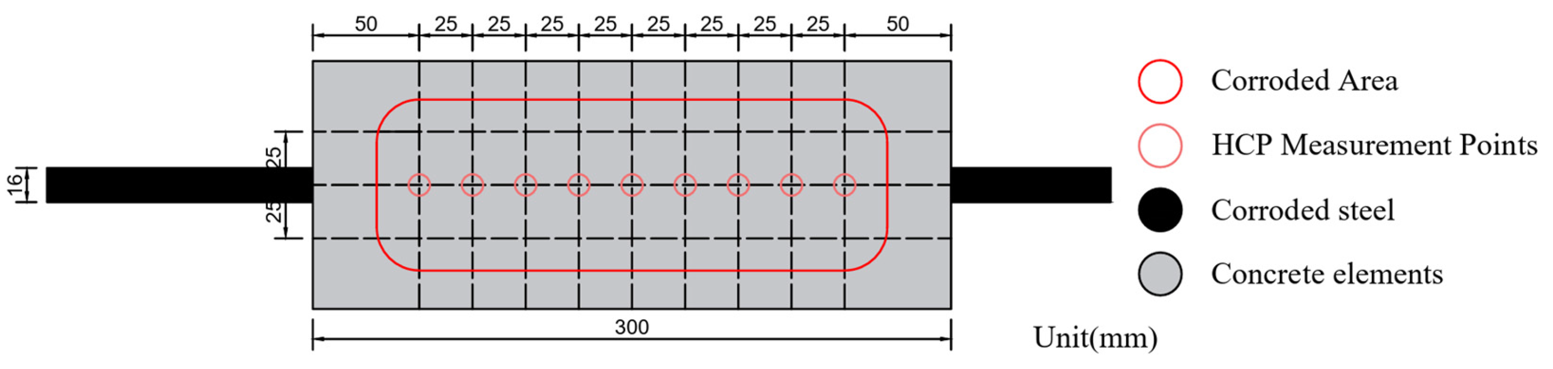
3.1. Specimen Design

Several reinforced concrete specimens were made and were used to conduct a constant-current accelerated corrosion test to explore the correlation between the half-cell potential and the corrosion ratio of reinforcing steels. The main ingredient of these concrete specimens was listed as follows. The cement was P. O 52.5. The fine aggregates in Zone II are medium sand. Its fineness modulus varies between 2.3 and 3.0, and its average particle size is 0.35 mm to 0.5 mm. The particle size of the coarse aggregate is 4.75 mm to 19.00 mm. The admixture was the performance water-reducing agent SF-J, and the admixture was 1.1%. The reinforcement bars embedded in the concrete are ribbed bars, and have a diameter of 12 mm and a yield strength of 345 MPa.

A larger water–binder ratio tends to increase the concrete’s void ratio, thereby accelerating reinforcement corrosion. Notwithstanding, the concrete’s water–binder ratio considerably affects the embedded reinforcement’s deterioration process. However, the sensitivity of the water–binder ratio in reflecting the rusting state was notably inferior to other parameters, such as the quality loss rate and cross-sectional loss rate, based on our thorough analysis of extensive electrochemical parameters from prior studies. Thus, the water–binder ratio was not incorporated into this experimental design.

Three groups of specimens were prepared using the mixing ratios listed in

Table 2. Mixture proportion of concrete [44].

Group	w/b	Amount of Materials Per Cubic Meter of Concrete/kg
		Cementitious Material (Cement)	Fine Aggregate (River Sand)	Coarse Aggregate (2#)	Water	Admixture
A	0.30	480	817	959	144	5.28
B	0.25	576	790	890	144	6.34
C	0.35	411	830	1015	144	4.52

. Group A was the baseline specimen (water–cement ratio w/b = 0.30; protective layer thickness of concrete c = 50 mm). Group B was a control specimen with w/b ratios (w/b = 0.25,0.35; c = 50 mm). Group C was the control specimen for the thickness of the protective layer (w/b = 0.30; c = 25 and 75 mm). Each specimen had a 16 mm diameter HRB rebar, for a total of 16 specimens in each group. The ends of the rebar protruding from the specimen were exposed to the air.

To prevent the corrosion of the exposed ends, they were pre-coated with epoxy resin and connected to two wires. One wire of each specimen was connected to the positive terminal of the DC power supply, and the other wire was connected to the negative terminal of the half-cell potentiometer to measure the half-cell potential during the accelerated corrosion test. The dimensions of the specimens are shown in Figure 1. And the schematic of HCP measurement is shown in Figure 2.

3.2. Accelerated Corrosion and HCP Test

After the specimens were maintained for 28 days, a 5% NaCl solution [5,45,46,47] was used for rinsing and immersion, thus inducing the corrosion of the reinforcement bars in the specimens. In this test, the corrosion of the steel bars in the specimens was accelerated using the constant current method [48,49,50]. The circuit is illustrated in Figure 3. Based on existing test experience [51,52,53,54,55,56], specimens with different corrosion rates were obtained by controlling the direct current density and energization duration according to Faraday’s law (Figure 4).

The direct current density was set to 0.20 mA/cm². Because the diameter of the reinforcement in the test piece was 16 mm and the proposed corrosion length range was 100 mm, the relationship between the corrosion mass loss m_r (g), corrosion duration T (s), and corrosion current I (A) can be determined by

$$m_r={\displaystyle \frac{TI\times 55.847}{2\times 96.487}}$$

(8)

Divided by the total mass of the steel bar in the specimen, the corroded mass reduction ratio ρ can be determined:

$$\rho ={\displaystyle \frac{m_r}{m_a}}={\displaystyle \frac{TI\times 55.847}{2\times 96.487\times 158}},$$

(9)

where m_a is the total mass of the non-corroded steel bar with a diameter of 16 mm and a length of 100 mm.

Despite the marked disparity in corrosion mechanisms between direct energized corrosion and those occurring in natural environments, the redox reaction inherent to rebar corrosion invariably results in a potential difference between the corroded and non-corroded sections of a rebar. The extent of this half-cell potential discrepancy accurately mirrors the corrosion severity of a rebar. Thus, while different corrosion mechanisms may induce variations in corrosion rates and morphologies between direct energized and naturally occurring corrosion, the half-cell potential measurements remain consistently indicative of the corrosion state [5,47]. This study primarily addresses the challenge of minimizing the subjective bias in model selection and the measurement inaccuracies associated with half-cell potential in determining the corrosion status of steel reinforcement. Consequently, employing half-cell potential data from samples subjected to energized corrosion does not compromise the integrity of the study’s findings.

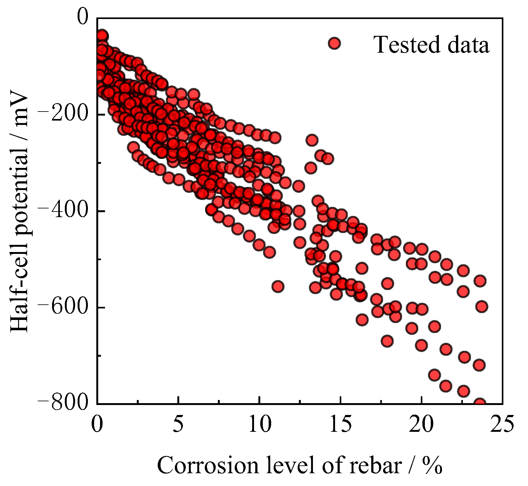
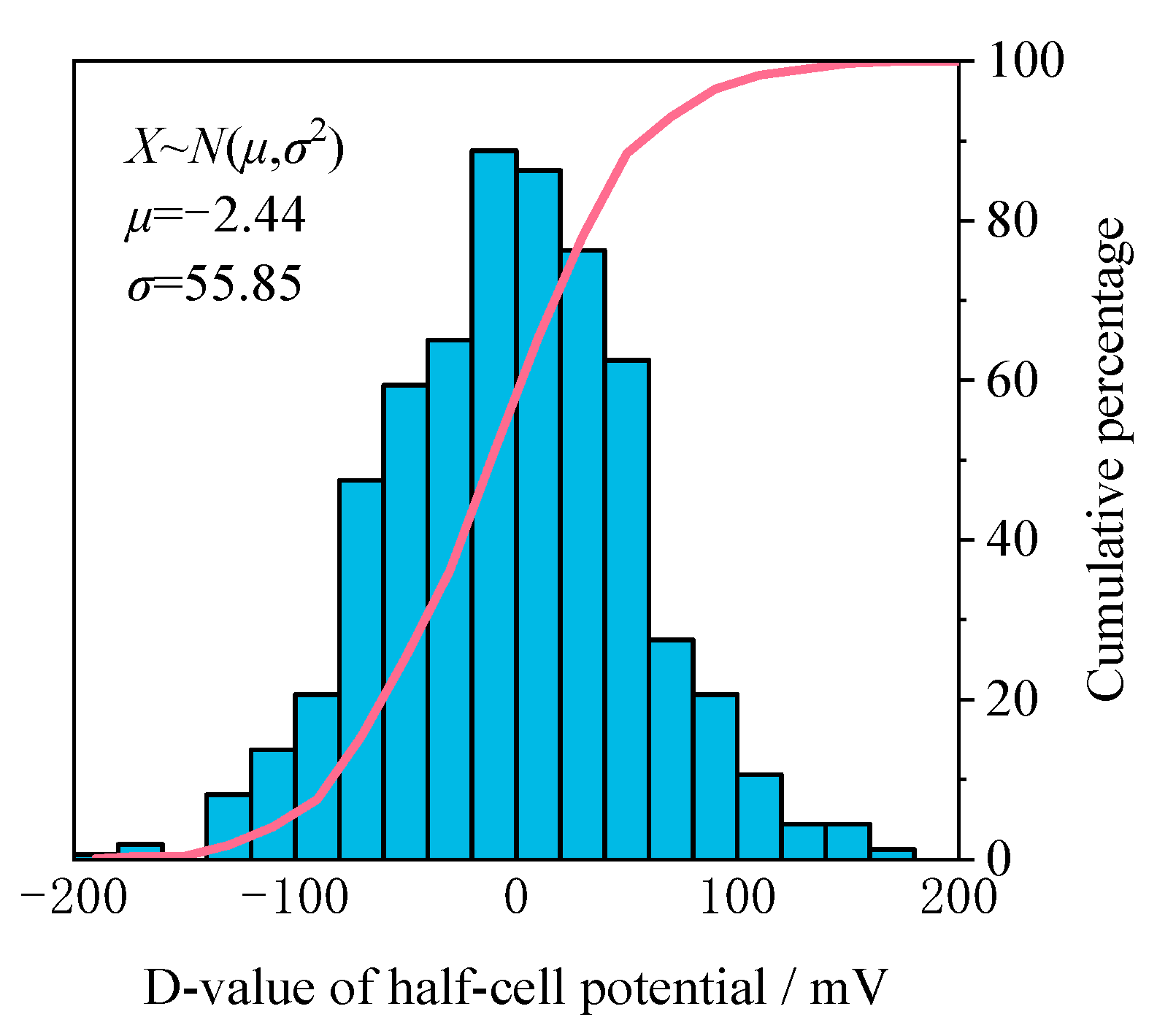
3.3. Data Collection

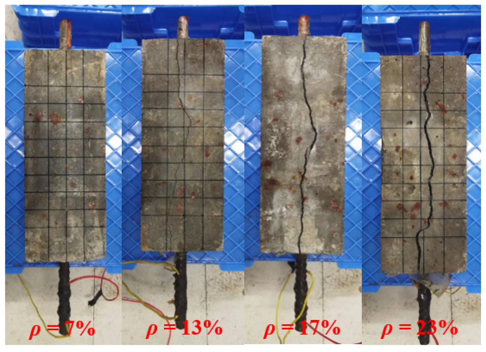
During the galvanic corrosion process, the specimens were placed in a uniform environment with a concrete moisture content of 50–60% and an ambient temperature of 20–25 °C. The specimens were then subjected to a galvanic corrosion process for 12 h, followed by depolarization (no current applied) for 12 h. Each specimen was subjected to 12 h of energized induced corrosion followed by 12 h of depolarization (no current applied), and the potential value of the reinforcement bar in each specimen was measured for the first time using an HC-X5 potential detector with a measuring range from −1000 mV to 1000 mV and an accuracy of ±1.0 mV. The detection area and locations of the detection points that satisfy the proposed corrosion length of 100 mm are shown in Figure 2. This energization and depolarization cycle was repeated until the specimen reached the set corrosion rates (7%, 13%, 17%, and 23%, respectively).

After reaching the specified corrosion level, specimens showing different corrosion rates were placed in controlled walk-in environmental chambers to allow for accurate HCP measurements under consistent environmental conditions. The HCP was taken as the average of five adjacent measurement points. Sixteen groups of specimens (corrosion rates of 7%, 13%, 17%, and 23%) were placed in an artificial indoor climate and environmental test chamber. The HCP measurements corresponding to these different corrosion rates were recorded at different humidity and temperature settings and carefully regulated in the chamber.

The effects of w/b, c, W, and T on the HCP test results were further investigated. Sixteen specimens from Group A with different corrosion rates were placed in an indoor artificial climate and environmental test chamber. The effects of W and T on the results of the HCP tests were then assessed by recording the HCP measurements corresponding to these different corrosion rates at W = 50% and T = 20 °C. The HCP measurements were then recorded at W = 50%, and T = 20 °C. Subsequently, by setting the same energizing voltage and energizing duration, six specimens in group B (for three, w/b = 0.25, for the other three, w/b = 0.35) and six specimens in group C (for three, c = 25 mm, and for the other three, c = 75 mm) were obtained. Potentiometric tests were conducted under similar conditions (corroded mass reduction ratio, water content, and temperature). The combination of the potential measurements of Group A specimens with corroded mass reduction ratios of 7%, 13%, 17%, and 23% was used to analyze the influence of the w/b ratio and thickness of the protective layer on the results of the potentiometric tests.

3.4. Test Results

A total of 456 sets of HCP test results were collected for the 16 standard specimens in Group A in a uniform environment, with each set of results corresponding to a different corrosion rate. Figure 5 shows the correlation between the HCP readings and the different levels of corrosion experienced by the specimens, with a clear trend. the HCP test results decreased as the corrosion rate of the reinforcement in the concrete increased. This observation agrees with the findings of Leelalerkiet et al. [4,5,6,7,8,9,57]. Similarly, Said et al. [58,59,60,61,62] found a direct relationship in which the lower the HCP was, the higher the corrosion rate of the reinforcement. In addition, as shown in Figure 6, the variance in the HCP test results from their mean values under uniform environmental conditions is closely related to the corrosion rate of the rebar, which is consistent with a Gaussian distribution. This distribution is characterized by a mean value of −2.44 and a standard deviation of 55.85. This deviation from the mean HCP value represents an objective uncertainty that is inherent in the test results, which significantly affects the development of accurate prediction models for corrosion assessment.

In order to discuss more succinctly the effects of various factors on HCP measurements, a baseline or “standard state” was set up with the parameters set to w/b = 0.30, c = 50 mm, W = 50%, and T = 20 °C. This benchmark condition was established to offer a standardized reference point, facilitating the comparison and analysis of diverse studies and engineering practices on an equal footing. These benchmark conditions draw upon typical values frequently cited in the literature. A water–cement ratio (w/c) of 0.30 was selected as the norm, as it is widely regarded to strike an optimal balance between the workability and strength properties of concrete. While this ratio does not signify any absolute physical attribute, it has been recognized through numerous studies and practical applications as a viable compromise that ensures both the requisite fluidity for ease of use and the durability and strength of the concrete [63]. A standard water content of 50% was determined to mimic a relatively stable internal environment of concrete under laboratory conditions, thereby enabling a more precise evaluation of concrete’s performance [64]. The thickness of the protective layer was determined by referencing similar specimens documented in the historical literature, typically ranging between 45 mm and 55 mm [65]. The chosen test temperature of 20 °C is derived from the optimal median values found in historical studies [66].

In the standard state, the HCP readings are taken at the same time as the HCP readings. The primary metric analyzed was the deviation of the other conditions from the HCP readings in this standard state. Figure 7 depicts the probability distribution of HCP deviations between the standard condition and the various test environments, water–cement ratios, and concrete cover depths, showing an approximate Gaussian distribution with a mean of 3.08 and a standard deviation of 91.42. The standard deviation of these differences increased by 63.7% compared with the results obtained under specific but similar environmental conditions, highlighting that the ambient humidity and temperature, depth of concrete cover, and water–cement ratio have a significant impact on HCP measurements. This large variation is coupled with the current debate regarding adjusting HCP values according to these factors [32,33,34,35]. The mean value of the differences shown in Figure 7 is almost zero. In probabilistic prediction models, the effects of these variables are categorized as subjective uncertainties. Therefore, the term γσ² was introduced in model Equation (4) to quantify these subjective uncertainties, indicating that they play a key role in the accuracy and reliability of HCP-based corrosion assessments.

4. Prior Correlation Model and Bayesian Updating

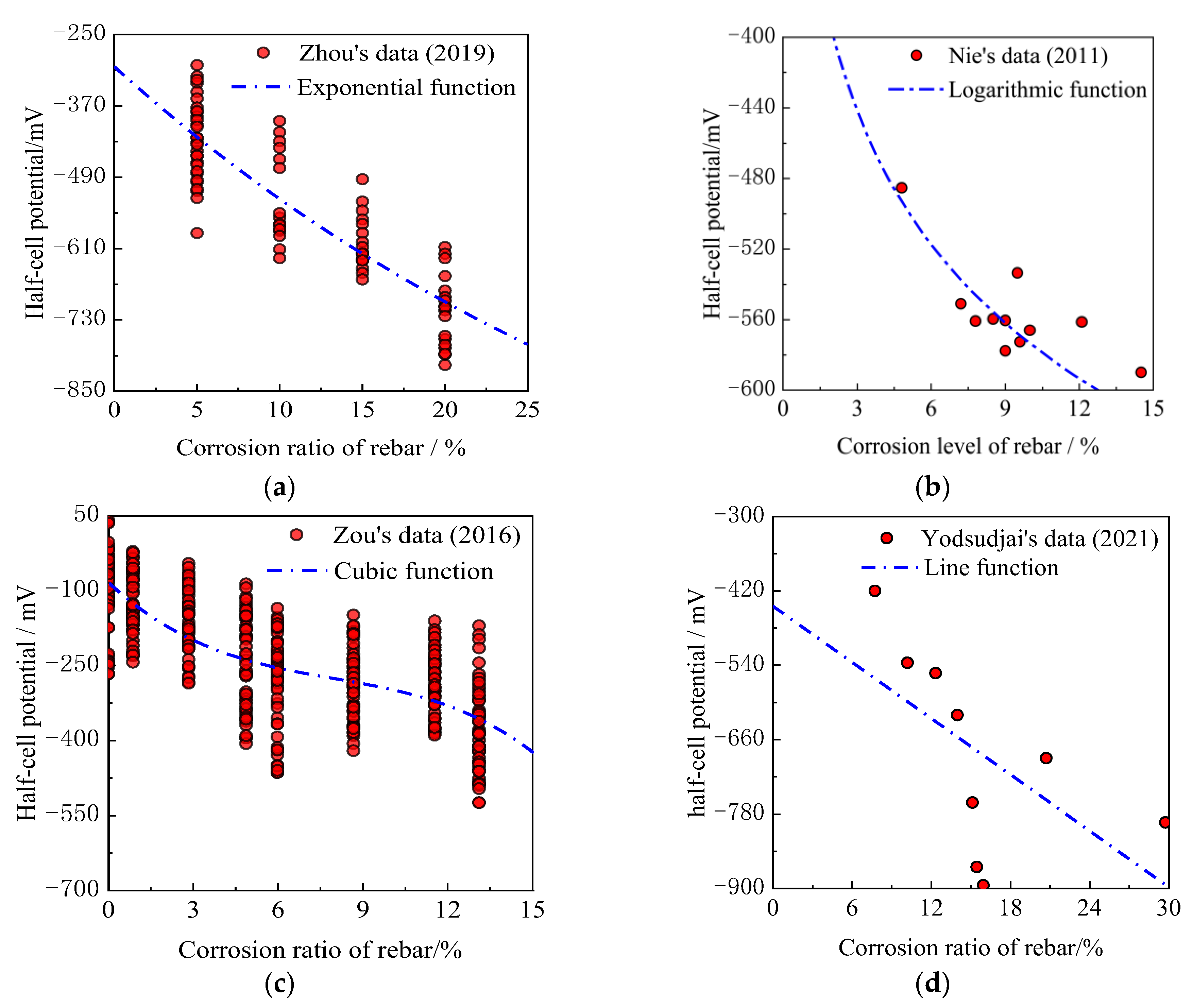
4.1. Prior Correlation Model

The correlation models in the published literature were selected as the prior models, as listed in

Table 3. The existing deterministic model of the relationship between HCP and the corroded mass reduction ratio.

No.	Function	Equation	Regression Parameters	Ref.
1	Exponential Function	$P=f_1\left(\rho \right)=a+b\cdot e^{\left(-\rho /c\right)}$	a = −1304.0, b = 1000.0, c = 39.7	[8]
2	Logarithmic Function	$P=f_2\left(\rho \right)=a\cdot \ln \left(\rho \right)+b$	a = −109.7, b = −320.7	[7]
3	Cubic Function	$P=f_3\left(\rho \right)=a\cdot {\rho }^3+b\cdot {\rho }^2+c\cdot \rho +d$	a = −0.22, b = 5.35, c = −52.39, d = −85.21	[5]
4	Linear Function	$P=f_4\left(\rho \right)=a\cdot \rho +b$	a = −15.1, b = −444.6	[9]

. The relevant test data and regression analysis results for the correlation models are shown in Figure 8.

Table 3 overlooks the critical impact of factors such as the water–cement ratio, concrete cover depth, ambient humidity, and temperature on the results of HCP tests, thereby neglecting the role of subjective uncertainties in corrosion prediction. Additionally, the reliance on a singular functional representation in these models fails to account for the inherent objective uncertainties arising from the limitations of model accuracy. Bayesian factors are introduced to facilitate a more nuanced analysis, enabling a comprehensive assessment that encompasses both subjective and objective uncertainties in the predictive framework.

$$P=X(M_1)\cdot f_1(\rho )+X(M_2)\cdot f_2(\rho )+X(M_3)\cdot f_3(\rho )+X(M_4)\cdot f_4(\rho )+\gamma {\sigma }^2,$$

(10)

where f₁–f₄ correspond to the exponential, logarithmic, cubic, and linear polynomial functions, respectively, in Table 3. The Bayesian factor X (M) was viewed as a random variable, whose prior probability distributions were assumed to follow a Gaussian distribution with a mean value of 1/4 and a variance of 1. As the Bayesian method was regarded as a progressive updating process with an increase in experimental data, we divided the 456 sets of experimental data obtained in test results into three subgroups evenly and randomly. Prior information on the Bayesian factors was fused with one subgroup to obtain a sequence of random samples of X (M) by adopting the MCMC method. Each Bayesian factor was sampled 100,000 times, and the sample sequence was constructed using the results of the last 90,000 iterations. This was performed to eliminate the influence of abnormal sample values obtained from the incomplete convergence of the Markov chain.

After random sample sequences of X (M) were obtained using the MCMC method, the Kolmogorov–Smirnov test was carried out on these sequences to obtain the distribution of X (M). The histograms and Q-Q diagrams of X (M₁) are shown in Figure 9.

The analysis of X (M) using histograms and Q-Q plots revealed that it adhered to a Gaussian distribution, characterized by a mean of 0.3833 and a variance of 0.0979. The application of the K-S test, on the sample sequences of X (M₁) yielded results exceeding 0.2. This result substantiates the Gaussian [67] nature of X (M₁) distribution. Similar methodologies were used to calculate the statistical attributes of the posterior distributions for the additional Bayesian factors.

Subsequent updates utilize the posterior distribution of X (M), derived from the latest update, as prior information. This prior distribution was then integrated with data from another subgroup to formulate a new posterior distribution for X (M). This iterative process is executed twice. Ultimately,

Table 4. The estimation of variables in the existing deterministic model of the relationship between HCP and the corroded mass reduction ratio.

Update Times	Update 1			Update 2			Update 3
Variables	Mean	Sd.	Distribution	Mean	Sd.	Distribution	Mean	Sd.	Distribution
θ1	0.3833	0.09789	Normal	0.4588	0.05626	Normal	0.4718	0.04179	Normal
θ2	0.0902	0.07506	Normal	0.0503	0.04343	Normal	0.0350	0.03193	Normal
θ3	0.2857	0.03663	Normal	0.2493	0.02296	Normal	0.2710	0.01819	Normal
θ4	0.0238	0.02382	Normal	0.0117	0.01163	Normal	0.0069	0.00688	Normal
σ	93.96	-	-	90.68	-	-	90.14	-	-

presents the characteristic statistical parameters for each Bayesian variable that capture the evolution of these parameters through consecutive updates.

The characteristic values of each Bayesian variable in Table 4 are plugged into Equations (6) and (7) to obtain the probabilistic distribution of HCP corresponding to different corroded mass reduction ratios. The variation in the probability density function of X (M) and potential prediction results (ρ = 7.5%) corresponding to the three Bayesian updating processes were plotted in Figure 10 and Figure 11, respectively.

As shown in

Table 5. Statistical information of the posterior distribution of parameters in different probability models. ① Exponential function; ② logarithmic function; ③ cubic function; ④ linear function.

Combination scheme of prior functions	①		②		③		④
Variables	θ1	γ	θ2	γ	θ3	γ	θ4	γ
Mean	0.7349	107.2	0.7025	129.0	0.7663	151.7	0.6307	131.0
Sd.	0.008523	-	0.009845	-	0.01299	-	0.00902	-
Distribution	Gaussian	-	Gaussian	-	Gaussian	-	Gaussian	-
Combination scheme of prior functions	① + ②			① + ③			① + ④
Variables	θ1	θ2	Γ	θ1	θ3	γ	θ1	θ4	γ
Mean	0.7315	0.007831	107.3	0.5216	0.2639	90.86	0.7334	0.005289	107.4
Sd.	0.01169	0.007752	-	0.01587	0.01708	-	0.01039	0.005235	-
Distribution	Gaussian	Gaussian	-	Gaussian	Gaussian	-	Gaussian	Gaussian	-
Combination scheme of prior functions	② + ③			② + ④			③ + ④
Variables	θ1	θ3	Γ	θ2	θ4	γ	θ3	θ4	γ
Mean	0.43	0.356	94.19	0.4632	0.2164	128.4	0.3525	0.3847	100.4
Sd.	0.01379	0.01544	-	0.08762	0.07879	-	0.01746	0.01404	-
Distribution	Gaussian	Gaussian	-	Gaussian	Gaussian	-	Gaussian	Gaussian	-
Combination scheme of prior functions	① + ② + ③				① + ② + ④
Variables	θ1	θ2	θ3	γ	θ1	θ2	θ4	γ
Mean	0.4829	0.03303	0.2697	90.97	0.7258	0.007592	0.005198	107.5
Sd.	0.03844	0.02991	0.01811	-	0.01284	0.007441	0.005186	-
Distribution	Gaussian	Gaussian	Gaussian	-	Gaussian	Gaussian	Gaussian	-
Combination scheme of prior functions	① + ③ + ④				② + ③ + ④
Variables	θ1	θ3	θ4	γ	θ2	θ3	θ4	γ
Mean	0.5131	0.2646	0.006872	90.99	0.4133	0.3547	0.01595	94.32
Sd.	0.01792	0.01717	0.006706	-	0.02135	0.01581	0.01512	-
Distribution	Gaussian	Gaussian	Gaussian	-	Gaussian	Gaussian	Gaussian	-

and Figure 10 and Figure 11, the variance of Bayesian factor X (M) and the mean value of σ gradually decrease by increasing the updating times, indicating that the posterior distribution of HCP gradually converges to a stable value with the rise in update times.

4.2. Accuracy Validation of the Proposed Prior Model

The validity of the probabilistic model delineated in the Prior Correlation Model was rigorously evaluated using an additional 100 groups of test data generated within this study, along with 80 groups of test data sourced from the existing literature [5,6,7,8,9,58,60,68]. These external samples exhibited a wide range of conditions, with corroded mass reduction ratios of reinforcement spanning 0 to 25.0%, moisture content between 25% and 65%, and ambient temperatures from 10 °C to 40 °C. The corrosion of reinforcements in RC structures or specimens is induced by two distinct methods: natural exposure tests and accelerated corrosion via direct current (DC) application. As illustrated in Figure 12 and Figure 13, the empirical data, both from this study and the referenced literature, consistently fell within the 95% confidence intervals predicted by the probabilistic model. Remarkably, the 50% confidence interval of the model illustrated over half of the test samples, underscoring its efficacy in capturing the intricate relationship between HCP and the corroded mass reduction ratio of the reinforcement in concrete. This comprehensive analysis substantiates that the probabilistic model offers a more accurate reflection of the underlying dynamics affecting HCP in the context of concrete corrosion.

The dispersion of the test data within the confidence intervals predicted by the probabilistic model emphasizes the random nature of the data, highlighting the effect of subjective and objective uncertainties—such as variations in test methods, inaccuracies in instrumental measurements, water–cement ratios, the depth of concrete cover, and test environments—on the quantitative relationship between the corroded mass reduction ratio and HCP. This probabilistic model correlates corroded mass reduction ratios with easily measurable or predictable parameters, making it useful for structural monitoring and assessment applications [14,30]. Confidence intervals, along with a reasonable level of accuracy, can effectively capture the extent to which factors such as concrete resistivity, ambient humidity, and temperature affect the HCP test results. Thus, quantifying the effect of these uncertainties on the predicted results through the establishment of confidence intervals is a reasonable approach.

4.3. Influence Analysis of Prior Information

Compared with the classical statistical approach, the Bayesian approach places greater emphasis on the impact of prior information on posterior outcomes. This posits that the uncertainty that is inherent in the selection of prior functions significantly affects the predictive accuracy of the model, often surpassing the influence of the independent variables. Despite the myriad of functions and their combinations available for use as prior functions, pinpointing the most suitable prior function based solely on expert judgment is challenging. Consequently, we employed permutation and combination techniques to derive diverse prior functions and subsequently performed Bayesian updating using the test samples discussed in ACCELERATED CORROSION TEST AND RESULT ANALYSIS. The resultant posterior probability distributions of the Bayesian factor X (M) across the various models after three rounds of updating are documented in Table 5. This approach underscores the nuanced consideration of prior knowledge in refining model predictions using the Bayesian methodology, showing its flexibility and depth in accommodating and quantifying uncertainties within the modeling process.

After comparing the prediction results of the above posterior probability models with identical samples as in the Accuracy Validation of The Proposed Prior Model Section, the adaptability evaluation of the prior information was conducted using the mean absolute error (MAE), root mean squared error (RMSE), coefficient of determination (R²), and other indicators [69], and the results were shown in

Table 6. Analysis of the fitting degree of probability prediction models with different a priori function combinations to test data.

Combination scheme of a priori functions	①	②	③	④	① + ②	① + ③	① + ④	② + ③
MAE	69.5	93.4	106.3	88.7	69.8	49.7	69.7	51.9
RMSE	88.9	116.9	129.8	111.8	89.2	61.6	89.1	64.6
R2	0.72	0.52	0.41	0.56	0.72	0.87	0.72	0.85
Mean width of 95% confidence interval/mV	420.6	506.1	595.2	513.9	421.6	363.0	421.7	371.5
Combination scheme of a priori functions	② + ④	③ + ④	① + ② + ④	① + ② + ④	① + ③ + ④	② + ③ + ④	① + ② + ③ + ④
MAE	91.6	56.5	49.8	69.9	49.8	52.1	50.0
RMSE	114.4	68.7	61.8	89.4	61.7	64.7	61.9
R2	0.54	0.84	0.87	0.72	0.87	0.85	0.87
Mean width of 95% confidence interval/mV	566.0	396.3	375.5	422.7	364.2	375.3	371.4

and

Table 7. Analysis of the fitting degree of probability prediction models with different a priori function combinations to literature data.

Combination scheme of a priori functions	①	②	③	④	① + ②	① + ③	① + ④	② + ③
MAE	60.9	71.9	106.1	106.1	61.1	48.4	61.0	50.5
RMSE	74.5	88.5	122.7	122.7	74.7	61.5	74.6	64.1
R2	0.57	0.39	<0.05	<0.05	0.57	0.71	0.57	0.68
Mean width of 95% confidence interval/mV	420.6	506.1	594.9	513.9	421.6	362.1	421.7	370.9
Combination forms of a priori functions	② + ④	③ + ④	① + ② + ④	① + ② + ④	① + ③ + ④	② + ③ + ④	① + ② + ③ + ④
MAE	69.8	52.0	48.5	61.1	48.5	50.4	48.6
RMSE	86.0	64.7	61.6	74.7	61.5	64.0	61.6
R2	0.43	0.68	0.71	0.57	0.71	0.68	0.71
Mean width of 95% confidence interval/mV	564.8	395.5	374.4	422.6	363.3	374.6	370.0

.

$$MAE={\displaystyle \frac{1}{n}}{\displaystyle \sum _{i=1}^{i=n}\left|P_i-P_i^P\right|}$$

(11)

$$RMSE=\sqrt{{\displaystyle \frac{1}{n}}{{\displaystyle \sum _{i=1}^{i=n}\left|P_i-P_i^P\right|}}^2}$$

(12)

$$R^2={\left[{\displaystyle \frac{n{\displaystyle \sum P_i\cdot }{P}_i^P-\left({\displaystyle \sum P_i}\right)\cdot \left({\displaystyle \sum P_i^P}\right)}{\sqrt{n\left({{\displaystyle \sum P_i}}^2\right)-n{\left({\displaystyle \sum P_i}\right)}^2}\cdot \sqrt{n\left({{\displaystyle \sum P_i^P}}^2\right)-n{\left({\displaystyle \sum P_i^P}\right)}^2}}}\right]}^2$$

(13)

Based on the definitions of MAE, RMSE, and R², it is established that lower MAE and RMSE values or a higher R² signify the enhanced adaptability of the prior model. Furthermore, a narrower confidence interval suggests a reduced likelihood of the prior model yielding erroneous conclusions. Table 6 illustrates that the MAE, RMSE, and average width of the 95% confidence intervals for the posterior model, which incorporates all four prior functions, were significantly lower than those for the posterior models referencing three or fewer prior functions. Although certain combinations of prior functions (① + ③, ① + ③ + ④) exhibit marginally superior performance compared to the integration of all four prior functions, identifying the most effective combination of prior functions for practical applications often poses a challenge. Moreover, the enhancements provided by these specific combinations were relatively modest. Therefore, augmenting the diversity of functions within the hybrid prior model can markedly reduce the objective uncertainty associated with the prior model, thereby increasing the predictive precision of the posterior model. This conclusion underscores the value of a comprehensive approach for selecting prior functions in Bayesian analysis and highlights its potential to refine and improve model predictions significantly.

4.4. Correlation Analysis of Corroded Mass Reduction Ratio and HCP

According to Equation (10) and the posterior probability distribution of X (M) in Table 4 and Table 5, the relationship between the corroded mass reduction ratio of the reinforcement and the HCP described by the posterior model corresponding to different function combinations was obtained, and the specific results are shown in Figure 14.

The test results depicted in Figure 14, along with the fitting outcomes presented in Figure 14, suggest a nuanced relationship between HCP and the corroded mass reduction ratio: HCP initially decreases gradually and then plummets markedly as the corroded mass reduction ratio increases. The hybrid prior model, comprising four distinct functions, demonstrated the most accurate correlation between the HCP and the corroded mass reduction ratio. In scenarios where the prior model is limited to a single function, exponential, logarithmic, and linear functions adequately capture the initial gentle decline in the HCP at lower corroded mass reduction ratios (<15%). Conversely, only the cubic polynomial function effectively represented the sharp decrease in the HCP observed at higher corroded mass reduction ratios (>15%). This differential capability underscores the necessity of including a cubic polynomial function within the prior model to attain an optimal fitting accuracy. Although the solitary use of a cubic polynomial function tends to underestimate the HCP at corroded mass reduction ratios below 15% and overestimate it beyond this threshold, incorporating Bayesian factors into the hybrid prior model rectifies these discrepancies, yielding a commendably accurate fit.

Moreover, when one Bayesian factor is three times greater than another, the contribution of the smaller factor can be disregarded in the composite function. However, if the ratio between the two Bayesian factors is within the range [1/3, 3], the influence of both functions on the predictive model becomes significant [70]. Given that the ratio of the Bayesian factor associated with the cubic polynomial function to that associated with the other functions resides within this critical interval, it is imperative to integrate the cubic polynomial function into the posterior model. This stipulation ensures a balanced and comprehensive representation of the relationship between the HCP and the corroded mass reduction ratio, enhancing the model’s predictive accuracy and reliability.

Because the gradient of the HCP with respect to the corroded mass reduction ratio varies significantly when the corroded mass reduction ratio is higher than 15%, it is appropriate to use a piecewise function to describe the relationship between the HCP and the corroded mass reduction ratio. The specific expressions are as follows:

$$P=\left\{\begin{array}{cc}X\left(M_1\right)\cdot f_1\left(\rho \right)+\gamma {\sigma }^2& \rho <15\%\\ X\left(M_1\right)\cdot f_1\left(\rho \right)+X\left(M_3\right)\cdot f_3\left(\rho \right)+\gamma {\sigma }^2& \rho \ge 15\%\end{array}\right.$$

(14)

The statistical analysis of X (M1) reveals that when the corroded mass reduction ratio is below 15%, it adheres to a normal distribution with a mean of 0.6500 and a variance of 0.008494, while σ follows a Gamma distribution with a mean of 84.01. Conversely, for corroded mass reduction ratios exceeding 15%, X (M₁) and X (M₃) both conform to Gaussian distributions, with means of 0.5337 and 0.2541, and variances of 0.04231 and 0.03196, respectively, and σ adheres to a Gamma distribution with a mean of 108.6. This delineation suggests that an exponential function accurately describes the decrease in the HCP relative to the corroded mass reduction ratio for values below 15%. In contrast, both an exponential function and a cubic polynomial function are required to encapsulate the relationship when the corroded mass reduction ratio exceeds 15%.

Evaluating the fitting performance shown in Figure 13, the piecewise function MAE was 51.2, and its RMSE was 63.9. Compared to a model that amalgamates four functions, the piecewise function shows a reduction in MAE and RMSE by 5.3% and 3.7%, respectively, along with a 5.1% decrease in the average width of the 95% confidence interval. These metrics strongly advocate for the adoption of a piecewise function to more accurately represent the correlation between the HCP and the corroded mass reduction ratio in reinforced concrete.

Moreover, the data from test results suggest a direct relationship between the reinforcement’s corroded mass reduction ratio and the variance in HCP test outcomes, with the width of the HCP’s confidence interval being nearly directly proportional to the corroded mass reduction ratio. For a comprehensive model encompassing all four functions, the 95% confidence interval width for the HCP at 0% corrosion was 361 mV, which increased by 11.6% as the corroded mass reduction ratio reached 25%. This trend is consistently reflected in the piecewise function, where in comparison to conditions with a corroded mass reduction ratio under 15%, the average 95% confidence interval width for HCP increases by approximately 28.8% for corroded mass reduction ratios greater than 15%. This observation underscores the capacity of the piecewise function to incorporate varying degrees of corroded mass reduction ratio impact, thereby enhancing its predictive accuracy and relevance.

5. Conclusions

In this study, an advancement over traditional deterministic models is demonstrated through the development of a probabilistic model that elucidates the relationship between the corroded mass reduction ratio of the reinforcement and HCP. By incorporating Bayesian factors, this model accurately navigates both objective uncertainties, such as flaws in experimental design and inaccuracies in measurements, and subjective uncertainties influenced by various factors in HCP measurements. Upon rigorous validation, the probabilistic model confirmed a gradual exponential decline in HCP with corroded mass reduction ratios below 15%, transitioning to a precipitous fall beyond this threshold. This behavior is depicted by a sophisticated blend of exponential and cubic polynomial functions, underscoring the complex dynamics between the HCP and corroded mass reduction ratios. This nuanced understanding highlights the necessity of employing a piecewise functional approach to capture this relationship accurately. Furthermore, the study revealed increasing variance and expanding confidence interval widths in HCP measurements revealed with rising corroded mass reduction ratios, emphasizing the critical importance of selecting appropriate deterministic model combinations from the literature to refine posterior predictions. Despite the limitations that are inherent in existing deterministic models to fully characterize the HCP–corroded mass reduction ratio relationship, the findings offer a pivotal foundation for enhancing durability assessments in reinforced concrete, paving the way for future investigations to further refine and expand upon this probabilistic model.

It should be emphasized that there is a robust correlation between the steel corrosion potential and the corrosion current density. Utilizing both the corrosion current density and potential allows for a more precise assessment of the corrosion status of steel embedded in concrete. However, due to the constraints of manuscript length, this aspect is not elaborated within this paper. It is anticipated that the simultaneous utilization of corrosion current density and corrosion potential merits as a valid approach to predict the corrosion state of steel bars.

References

1. Rodriguez, D.; Ortega, L.; Casal, J. Load carrying capacity of concrete structures with corroded reinforcement. Constr. Build. Mater. 1997, 11, 239–248. [Google Scholar] [CrossRef]
2. Cabrera, J. Deterioration of concrete due to reinforcement steel corrosion. Cem. Concr. Compos. 1996, 18, 47–59. [Google Scholar] [CrossRef]
3. Assouli, B.; Ballivy, G.; Rivard, P. Influence of environmental parameters on application of standard ASTM C876-91: Half-cell potential measurements. Corrosion Engineering. Sci. Technol. 2009, 43, 93–96. [Google Scholar] [CrossRef]
4. Wilson, J.M. Modeling Half-Cell Potentials and Their Relationship to Corrosion of Reinforcing Steel. Master’s Thesis, University of Massachusetts Lowell, Lowell, MA, USA, 2013. [Google Scholar]
5. Zou, Z.H.; Wu, J.; Wang, Z.; Wang, Z. Relationship between half-cell potential and corrosion level of rebar in concrete. Corros. Eng. Sci. Technol. 2016, 51, 588–595. [Google Scholar] [CrossRef]
6. Yodsudjai, W.; Pattarakittam, T. Factors influencing half-cell potential measurement and its relationship with corrosion level. Measurement 2017, 104, 159–168. [Google Scholar] [CrossRef]
7. Nie, Z.H.; Wu, J. Potential, resistivity and the relationship between the corrosion rate of steel. Low. Temp. Arch. Technol. 2011, 10, 6–8. [Google Scholar]
8. Zhou, Y. Study on Bond Behavior of Corroded Reinforced Concrete in Marine Environment: Degradation Law and Variability. Ph.D. Thesis, Shenzhen University, Shenzhen, China, 2019. [Google Scholar]
9. Yodsudjai, W.; Vanrak, P.; Suwanvitaya, P.; Jutasiriwong, A. Corrosion behavior of reinforcement in concrete with different compositions. J. Sustain. Cem.-Based Mater. 2021, 10, 129–148. [Google Scholar] [CrossRef]
10. Gonzalez, J.A.; Miranda, J.M.; Feliu, S. Considerations on reproducibility of potential and corrosion rate measurements in reinforced concrete. Corros. Sci. 2004, 46, 2467–2485. [Google Scholar] [CrossRef]
11. Almashakbeh, Y.; Saleh, E.; Al-Akhras, N. Evaluation of Half-Cell Potential Measurements for Reinforced Concrete Corrosion. Coatings 2022, 12, 975. [Google Scholar] [CrossRef]
12. Guo, R.; Guo, Z.; Yao, G.; Jin, Y.; Liu, Z. Hybrid prediction model for reinforcements’ corrosion stage by multiple nondestructive electrochemical indices. J. Build. Eng. 2024, 82, 108327. [Google Scholar] [CrossRef]
13. Aridas, C.; Karlos, S.; Kanas, V.; Fazakis, N.; Kotsiantis, S. Uncertainty Based Under-Sampling for Learning Naive Bayes Classifiers Under Imbalanced Data Sets. IEEE Access 2020, 8, 2122–2133. [Google Scholar] [CrossRef]
14. Ghods, P.; Isgor, O.; Pour-Ghaz, M. Experimental verification and application of a practical corrosion model for uniformly depassivated steel in concrete. Mater. Struct. 2007, 41, 1211–1223. [Google Scholar] [CrossRef]
15. Xia, J.; Shen, J.; Li, T.; Jin, W. Corrosion prediction models for steel bars in chloride-contaminated concrete: A review. Mag. Concr. Res. 2022, 74, 123–142. [Google Scholar] [CrossRef]
16. Song, H.-W.; Saraswathy, V. Corrosion monitoring of reinforced concrete structures—A review. Int. J. Electrochem. Sci. 2007, 2, 1–28. [Google Scholar] [CrossRef]
17. Adriman, R.; Ibrahim, I.B.M.; Huzni, S.; Fonna, S.; Ariffin, A.K. Improving half-cell potential survey through computational inverse analysis for quantitative corrosion profiling. Case Stud. Constr. Mater. 2022, 16, e00854. [Google Scholar] [CrossRef]
18. Mancio, M.; Carlos, C., Jr.; Zhang, J.; Harvey, J.T.; Monteiro, P.J.; Ali, A. Laboratory Evaluation of Corrosion Resistance of Steel Dowels in Concrete Pavement; University of California Pavement Research Center: Davis, CA, USA, 2005. [Google Scholar]
19. Angst, U.; Büchler, M. On the applicability of the Stern–Geary relationship to determine instantaneous corrosion rates in macro-cell corrosion. Mater. Corros. 2015, 66, 1017–1028. [Google Scholar] [CrossRef]
20. Hidenobu, T.; Takahiko, S. Studies on diagnosis and repair for reinforcing bar corrosion by salt injury. Trans. Jpn. Concr. Inst. 2001, 22, 211–220. [Google Scholar]
21. Sofiani, F.M.; Tacq, J.; Elahi, S.A.; Chaudhuri, S.; De Waele, W. A hybrid probabilistic-deterministic framework for prediction of characteristic size of corrosion pits in low-carbon steel following long-term seawater exposure. Corros. Sci. 2024, 232, 112039. [Google Scholar] [CrossRef]
22. Ma, Y.; Che, Y.; Gong, J. Behavior of corrosion damaged circular reinforced concrete columns under cyclic loading. Constr. Build. Mater. 2012, 29, 548–556. [Google Scholar] [CrossRef]
23. Nasser, H.V.; Vrijdaghs, R. Experimental investigation of corrosion damage on reinforced concrete beams to correlate crack width and mass loss. In Bridge Maintenance, Safety, Management, Life-Cycle Sustainability and Innovations; CRC Press: Boca Raton, FL, USA, 2021; pp. 2927–2934. [Google Scholar]
24. Zhao, Z.; Zhang, H.; Xian, L.; Liu, H. Tensile strength of Q345 steel with random pitting corrosion based on numerical analysis. Thin-Walled Struct. 2020, 148, 106579. [Google Scholar] [CrossRef]
25. Ge, X.; Dietz, M.; Alexander, N.; Kashani, M. Nonlinear dynamic behaviour of severely corroded reinforced concrete columns: Shaking table study. Bull. Earthq. Eng. 2019, 18, 1417–1443. [Google Scholar] [CrossRef]
26. Mei, K.; He, Z.; Yi, B.; Lin, X.; Wang, J.; Wang, H.; Liu, J. Study on electrochemical characteristics of reinforced concrete corrosion under the action of carbonation and chloride. Case Stud. Constr. Mater. 2022, 17, e01351. [Google Scholar] [CrossRef]
27. Woo, B.-H.; Lee, J.; Kim, J.; Kim, H. Corrosion state assessment of the rebar via Bayesian inference. Constr. Build. Mater. 2023, 392, 131791. [Google Scholar] [CrossRef]
28. Lee, H.-S.; Kim, H.G.; Ryou, J.-S.; Kim, Y.; Woo, B.-H. Corrosion state assessment of the rebar: Experimental investigation by ambient temperature and relative humidity. Constr. Build. Mater. 2023, 408, 133598. [Google Scholar] [CrossRef]
29. Muthulingam, S.; Rao, B. Non-uniform corrosion states of rebar in concrete under chloride environment. Corros. Sci. 2015, 93, 267–282. [Google Scholar] [CrossRef]
30. Song, L.; Liu, J.; Liu, R.; Sun, H.; Yu, Z. Unification and calibration of steel corrosion models based on long-term natural corrosion. Constr. Build. Mater. 2024, 411, 134611. [Google Scholar] [CrossRef]
31. Yao, L. Experimental Study on Bond Performance of Corroded Reinforced Concrete Under Fatigue Loading. Master’ Thesis, Shenzhen University, Shenzhen, China, 2020. [Google Scholar]
32. Poursaee, A.; Hansson, C. Potential pitfalls in assessing chloride-induced corrosion of steel in concrete. Cem. Concr. Res. 2009, 39, 391–400. [Google Scholar] [CrossRef]
33. Pour-Ghaz, M.; Isgor, O.; Ghods, P. Quantitative Interpretation of Half-Cell Potential Measurements in Concrete Structures. J. Mater. Civ. Eng. 2009, 21, 467–475. [Google Scholar] [CrossRef]
34. Reichling, K.; Raupach, M.; Broomfield, J.; Gulikers, J.; L’Hostis, V.; Kessler, S.; Osterminski, K.; Pepenar, I.; Schneck, U.; Sergi, G.; et al. Full surface inspection methods regarding reinforcement corrosion of concrete structures. Mater. Corros.-Werkst. Und Korros. 2013, 64, 116–127. [Google Scholar] [CrossRef]
35. Koga, G.; Albert, B.; Nogueira, R. Revisiting the ASTM C876 standard for corrosion of reinforcing steel: On the correlation between corrosion potential and polarization resistance during the curing of different cement mortars. Electrochem. Commun. 2018, 94, 1–4. [Google Scholar] [CrossRef]
36. Kim, Y.; Kim, J.; Bang, J.; Kwon, S. Effect of cover depth, w/c ratio, and crack width on half-cell potential in cracked concrete exposed to salt sprayed condition. Constr. Build. Mater. 2014, 54, 636–645. [Google Scholar] [CrossRef]
37. Su, J.; Yang, C.; Wu, W.; Huang, R. Effect of Moisture Content on Concrete Resistivity Measurement. J. Chin. Inst. Eng. 2002, 25, 117–122. [Google Scholar] [CrossRef]
38. Elsener, B.; Andrade, C.; Gulikers, J. Half-cell potential measurements—Potential mapping on reinforced concrete structures, recommendations. Mater. Struct. 2003, 36, 461–471. [Google Scholar] [CrossRef]
39. Haenni, R.; Romeijn, J.; Wheeler, G.; Williamson, J. Probabilistic Logics and Probabilistic Networks; Springer: Dordrecht, The Netherlands, 2011. [Google Scholar]
40. Wang, S. Learning, Reasoning and Application of Bayesian Network; Lixin Accounting Press: Shanghai, China, 2010. [Google Scholar]
41. Brooks, S.; Gelman, A.; Jones, G.; Meng, X. Handbook of Markov Chain Monte Carlo; Taylor and Francis; CRC Press: New York, NY, USA, 2011. [Google Scholar]
42. Mao, S.; Tang, Y. Bayesian Statistics; China Statistics Press: Beijing, China, 2012. [Google Scholar]
43. Boslaugb, S. Statistics in a Nutshell Second Edition; O’Reilly Media, Inc.: Sebastopol, CA, USA, 2012. [Google Scholar]
44. Guo, Z.; Guo, R.; Yao, G. Bayesian Probabilistic Model for Reinforcement Corrosion Ratio of Reinforcement in Concrete Prediction Based on Modified Half-cell Potential. J. Civ. Struct. Health. 2024, 14, 485–500. [Google Scholar] [CrossRef]
45. Li, Q.; Dong, Z.; He, Q.; Fu, C.; Jin, X. Effects of Reinforcement Corrosion and Sustained Load on Mechanical Behavior of Reinforced Concrete Columns. Materials 2022, 15, 3590. [Google Scholar] [CrossRef]
46. Xia, J.; Jin, W.; Li, L. Shear performance of reinforced concrete beams with corroded stirrups in chloride environment. Corros. Sci. 2011, 53, 1794–1805. [Google Scholar] [CrossRef]
47. Ye, Z.; Zhang, W.; Gu, X. Deterioration of shear behavior of corroded reinforced concrete beams. Eng. Strut. 2018, 168, 708–720. [Google Scholar] [CrossRef]
48. Yuan, Y.; Zhang, X.; Ji, Y. A comparative study on structural behavior of deteriorated reinforced concrete beam under two different environments. China Civ. Eng. J. 2006, 39, 42–46. [Google Scholar]
49. Fan, L.; Tan, X.; Zhang, Q.; Meng, W.; Chen, G.; Bao, Y. Monitoring corrosion of steel bars in reinforced concrete based on helix strains measured from a distributed fiber optic sensor. Eng. Struct. 2020, 204, 110039. [Google Scholar] [CrossRef]
50. Sun, Y.; Qiao, G. Influence of Constant Current Accelerated Corrosion on the Bond Properties of Reinforced Concrete. Int. J. Electrochem. Sci. 2019, 14, 4580–4594. [Google Scholar] [CrossRef]
51. Sun, J. Fatigue Behavior Analysis, Safety and Durability Assessment of Corroded RC Beam Bridges in Coastal Area. Ph.D. Thesis, Southeast University, Nanjing, China, 2016. [Google Scholar]
52. Chen, C. Experimental Research on Fatigue Performance of Reinforced Concrete Beams Under Overload and Corrosion Damage. Master’s Thesis, Zhejiang University, Hangzhou, China, 2015. [Google Scholar]
53. Williamson, S.; Du, Y.G.; Clark, L.A. Deflection of RC beams under simultaneous load and steel corrosion. Mag. Concr. Res. 2003, 55, 405–406. [Google Scholar] [CrossRef]
54. Higgins, C.; Ii, W. Tests of Reinforced Concrete Beams with Corrosion-Damaged Stirrups. ACI Struct. J. 2006, 103, 133–141. [Google Scholar]
55. Minh, H.; Mutsuyoshi, H.; Niitani, K. Influence of grouting condition on crack and load-carrying capacity of post-tensioned concrete beam due to chloride-induced corrosion. Constr. Build. Mater. 2005, 21, 1568–1575. [Google Scholar] [CrossRef]
56. Yi, W.J.; Zhao, X. The effect of bar corrosion on the performance of reinforced concrete beams under long-term load. China Civ. Eng. J. 2006, 39, 7–12. [Google Scholar]
57. Leelalerkiet, V.; Kyung, J.; Ohtsu, M.; Yokota, M. Analysis of half-cell potential measurement for corrosion of reinforced concrete. Constr. Build. Mater. 2004, 18, 155–1623. [Google Scholar] [CrossRef]
58. Said, M.; Hussein, A. Induced Corrosion Techniques for Two-Way Slabs. J. Perform. Constr. Facil. 2019, 33, 04019026. [Google Scholar] [CrossRef]
59. Abouhussien, A.; Hassan, A. Evaluation of damage progression in concrete structures due to reinforcing steel corrosion using acoustic emission monitoring. J. Civ. Struct. Health Monit. 2015, 5, 751–765. [Google Scholar] [CrossRef]
60. Yoon, S.; Wang, K.; Weiss, W. Interaction between Loading, Corrosion, and Serviceability of Reinforced Concrete. ACI Mater. J. 2000, 97, 637–644. [Google Scholar] [CrossRef]
61. Zhang, J.; Ma, H.; Pei, H.; Li, Z. Steel corrosion in magnesia-phosphate cement concrete beams. Mag. Concr. Res. 2017, 69, 35–45. [Google Scholar] [CrossRef]
62. Jin, W.; Wang, Y. Experimental study on mechanics behaviors of reinforced concrete beams under simultaneous chloride attacks and sustained load. J. Zhejiang Univ. Eng. Sci. 2014, 48, 221–227. [Google Scholar]
63. Lu, Z.; Lun, P.; Li, W.; Luo, Z.; Li, Y.; Liu, P. Empirical model of corrosion rate for steel reinforced concrete structures in chloride-laden environments. Adv. Struct. Eng. 2019, 22, 223–239. [Google Scholar] [CrossRef]
64. Chun, P.; Ujike, I.; Mishima, K.; Kusumoto, M.; Okazaki, S. Random forest-based evaluation technique for internal damage in reinforced concrete featuring multiple nondestructive testing results. Constr. Build. Mater. 2020, 253, 119238. [Google Scholar] [CrossRef]
65. Zhang, H.; Qi, J.; Zheng, Y.; Zhou, J.; Qiu, J. Characterization and grading assessment of rebar corrosion in loaded RC beams via SMFL technology. Constr. Build. Mater. 2024, 411, 134484. [Google Scholar] [CrossRef]
66. Zhu, H.; Liu, X.; Jia, C.; Du, B.; Liu, S.; Qian, Y. An experimental study on the corrosion amount using a statistical analysis, Corrosion Engineering. Sci. Technol. 2018, 53, 26–35. [Google Scholar] [CrossRef]
67. Wu, J.; Zhang, X.; Guo, L.; Jin, L.; Du, X. Probabilistic bond strength prediction between the corroded reinforcing bars and concrete considering the concrete strength and non-uniform corrosion. Constr. Build. Mater. 2022, 357, 129338. [Google Scholar] [CrossRef]
68. Ji, C.; Song, J.; Liu, Y. Corrosion of internal rebar of recycled aggregate thermal insulation concrete under carbonization. Concrete 2020, 2, 13–16. [Google Scholar]
69. Cai, R.; Han, T.; Liao, W.; Huang, J.; Li, D.; Kumar, A.; Ma, H. Prediction of surface chloride concentration of marine concrete using ensemble machine learning. Cem. Concr. Res. 2020, 136, 106164. [Google Scholar] [CrossRef]
70. Zhang, C. A Study on Parameter Estimation and Model Selection Based on Approximate Bayesian Computation. Master’s Thesis, Hefei University of Technology, Hefei, China, 2019. [Google Scholar]
Figure 1. Reinforced concrete specimens.
Buildings 15 02095 g001
Figure 2. Schematic of HCP measurement.
Buildings 15 02095 g002
Figure 3. Diagram of galvanostatic method.
Buildings 15 02095 g003
Figure 4. Specimens with different degrees of corrosion [44].
Buildings 15 02095 g004
Figure 5. Corrosion state of rebar in concrete vs. half-cell potential.
Buildings 15 02095 g005
Figure 6. Statistical histogram of the difference between HCP test results and their mean value under the same condition with the corrosion rate of reinforcement.
Buildings 15 02095 g006
Figure 7. Statistical histogram for the differences in HCP test results between the standard state and the states with the different influence factors.
Buildings 15 02095 g007
Figure 8. Fitting data and results for each deterministic model. (a) Exponential function; (b) logarithmic function; (c) cubic function; and (d) linear function. (The mentioned references are [5,7,8,9]).
Buildings 15 02095 g008
Figure 9. Statistical report chart of parameter X (M1) [44]. (a) Histogram and (b) Q-Q figure.
Buildings 15 02095 g009
Figure 10. Update processes of the PDF for X (M). (a) X (M1); (b) X (M2); (c) X (M3); and (d) X (M4).
Buildings 15 02095 g010
Figure 11. Update processes of the PDF for P.
Buildings 15 02095 g011
Figure 12. Distribution of the manuscript’s tested data within the confidence interval [44].
Buildings 15 02095 g012
Figure 13. Distribution of the literature’s tested data within the confidence interval.
Buildings 15 02095 g013
Figure 14. Relationship between HCP and the corroded mass reduction ratio corresponding to the different priori functions.
Buildings 15 02095 g014