Abstract
Mid-deep geothermal heat pump systems (MD-GHPs) feature high energy efficiency and low energy consumption, yet their promotion is restricted by high initial investment. While the initial investment of air-source heat pumps (ASHPs) is obviously lower, it also has a larger energy consumption. To address the complementary strengths and weaknesses of single-source heat pump systems, this paper puts forward an integrated system combining MD-GHPs and ASHPs, and the series mode was determined as the optimal integration approach for the hybrid system through comparative analysis. Simulation analysis was conducted to explore the adaptability of series mode, and numbers of mid-deep ground heat exchangers in nine cities across various climate regions were studied. The MD-GHP system is suitable for space heating in Xining and Xi’an, while ASHPs are suitable for space heating in Nanjing and Hangzhou. For intermediate resource areas like Urumqi and Tsingdao, the series mode achieves the best economic benefits during the 24th year of operation.
1. Introduction
China’s building heating demand exhibits extensive distribution, with substantial energy consumption and rapid growth [1]. Particularly for space heating demand lacking clean waste heat, the low-carbon heating demand area exceeds 10 billion m2 [2]. Traditional heating methods like electric boilers and gas boilers would exacerbate environmental pollution and significantly increase carbon emissions. In recent decades, a heating technology that extracts mid-deep geothermal energy through mid-deep borehole heat exchangers (MDBHEs), and combined with electric-driven heat pump systems (MD-GHPs), has been increasingly promoted and applied in China. Numerous research studies have been conducted from fundamental theories to engineering applications, including the practical operation performance, heat transfer mechanisms of MDBHEs, and system optimization of the MD-GHPs [3].
To assess the operational efficiency of MDBHEs, extensive field evaluations have been systematically implemented across China. Deng [4,5] carried out comprehensive on-site measurements to study the operational characteristics of MDBHE under different operation modes. Results show that a single 2500 m MDBHE could achieve a 500 kW heat extraction capacity in continuous mode, with a water flow rate of 30 m3/h and an inlet water temperature of 5 °C [4]. Then, the heat extraction capacity could further elevate beyond 600 kW using the intermittent operation mode [5]. Moreover, an 1800 m MDBHE installed in Beijing [6] could operate stably with a heat extraction capacity of about 237.2–256.5 kW under water flow rates between 20 and 25 m3/h. Additionally, Wang et al. [7] examined a 2000 m MDBHE during a 5-day continuous operation cycle, where the average inlet and outlet water temperatures reached 17.5 °C and 26.7 °C, with a mean heat extraction capacity of 286.4 kW per MDBHE, coupled with the heat pump coefficient of performance (COP) of 6.4, showing better energy performance than other space heating technologies.
Numerous simulation analyses have been carried out based on measurement results to further investigate the operational characteristics of MDBHEs [8,9,10]. Findings indicate that three critical factors govern the heat extraction performance, including the geological thermal properties, the thermo-physical characteristics of the system, and operational parameters. Regarding geological parameters, enhanced heat extraction capacity correlates strongly with higher ground thermal conductivity [10] and ground temperature gradients [11]. Notably, groundwater seepage improves heat transfer efficiency during the heating season and accelerates ground temperature recovery during non-heating periods [12]. From the perspective of thermophysical characteristics, the increased borehole depth, larger pipe diameters, and the larger annulus tube and the smaller inner tube conductivity collectively enhance heat transfer performance [13,14]. Operational analysis reveals that the larger water flow rate and smaller inlet water temperature both contribute to the larger heat extraction capacities [15]. Recent investigations into operational protocols further demonstrate that intermittent operational modes outperform continuous modes, achieving 18–23% greater heat extraction capacity while simultaneously facilitating ground thermal recovery [16,17]. Additionally, the arrangement methods and space lines of MDBHE arrays also have a significant influence on the heat extraction capacity in long-term operation [18], and a line spacing of greater than 30 m was suggested to optimize system performance.
As for the energy performance of MD-GHPs, most researchers have focused on the system configuration and control optimizations. Wang investigated the operational performance of different heat pump types in MD-GHPs [19]. The results indicated that the constant-speed screw heat pumps fail to match the variations in heating capacity and compression ratio, resulting in the energy efficiency of whole system lower than 5.0. In contrast, variable-frequency centrifugal heat pumps achieve an EER of 7.0 through compressor speed adjustment to accommodate operational variations. Deng [20] optimized the performance of the MD-GHPs, including the heat pump system’s configuration. The results showed that the magnetic-bearing variable-speed centrifugal heat pump showed high efficiency under a wide range of heating loads and compression ratios, with an average COP of 6.21. Moreover, the two heat pumps operated in series further increased the average COP to 6.97. As for the system optimization, Wang [21] developed a hybrid MDBHE heating system with direct heating and coupled heat pump approaches. The results showed that the MDBHEs could operate independently for a few days at the beginning of the heating season, thus decreasing the energy consumption of the MD-GHPs. He [22] investigated the energy performance of a hybrid shallow and mid-deep geothermal heat pump system. The results showed that when the heating-to-cooling load ratio reached 1:2, the hybrid system exhibited 5.8% lower energy consumption. Therefore, the hybrid system is more suitable for applications with larger space heating demands than cooling demands. Li [23] addressed the decay of the heat extraction capacity of MDBHEs by investigating a photovoltaic/thermal-coupled medium-deep ground-source heat pump (PV/T-GSHP) system and a photovoltaic-assisted medium-deep ground-source heat pump combined with an air-source heat pump (PVGSHP-ASHP) system. The results indicated that after 20 years of operation, the PV/T-GSHP system slightly increased the soil temperature by 0.09 °C. Additionally, the PVGSHP-ASHP system alleviated soil temperature decline by load-sharing, while demonstrating energy efficiency.
In summary, the MD-GHPs struggle to balance low construction costs, high operational efficiency, and long-term stability. Previous studies have focused on enhancing equipment performance, optimizing control strategies, and multi-energy integration. However, there is a lack of comparative studies on varying heating demands, construction costs, and operational performance across different regions. Therefore, this paper conducted a simulation analysis to study the energy performance and economic feasibility of MD-GHPs in different regions of China. Then, the hybrid system combining MD-GHPs and ASHPs is proposed to compensate for the limitations of single heating sources and offer critical insights for advancing low-carbon and clean heating solutions
2. Methodology
2.1. Simulation Models Description
Considering the characteristics of MD-GHPs and ASHPs, as well as practical construction and operational feasibility, this paper proposes two hybrid system configurations, including the parallel mode, series mode, and cascade mode.
Figure 1a shows the system diagram and simulation model configuration of the series mode, where the condensers of MD-GHPs and ASHPs are connected in series, with the ASHPs’ condenser outlet water serving as the inlet water to the condenser of MD-GHPs. The outlet water temperature from ASHPs (Tc,o,a) is set based on the load distribution ratio under a fixed 5 °C user-side water temperature difference. Also, the heat demand model calculates the space heating loads and their distribution (Qc, Qc,m, Qc,a), as well as the condensing-side water temperatures (Tc,o, Tc,i, Tc,o,a). With the above parameters input to the models of MD-GHPs and ASHPs, the heat extraction capacities (Qe,m, Qe,a), power consumptions (Whpm, Whpa), and energy performance of heat pumps in MD-GHPs and ASHPs (COPm, COPa) could be calculated. The model of MDBHEs is the same as the parallel mode.
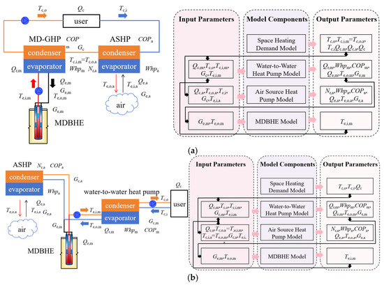
Figure 1.
System diagram and simulation model configuration: (a) Series mode; (b) Cascade mode.
Figure 1b shows the system diagram and simulation model configuration of the cascade mode, where the ASHPs replace part of the MDBHEs and serve as the heat source of the MD-GHPs. In this configuration, the ASHPs’ condenser side circulating water temperature matches the MDBHEs’ circulating water temperature, with the ASHPs’ heating capacity contributing to the heat extraction of the water-to-water heat pumps. The heat demand model calculates space heating load (Qc) and condensing-side water temperatures (Tc,o,Tc,i). Then, the water-to-water heat pump model calculates the heat extraction quantities (Qe), power consumptions (Whpw), and energy performance of the heat pump (COPw). Moreover, the evaporator side model of the water-to-water heat pump is specially designed so that the Qe is distributed to MDBHEs and ASHPs. The outlet water temperature from the evaporator of water-to-water heat pumps serves as the inlet water temperature of the MDBHEs. The evaporator-side water flow rates are distributed to MDBHEs and ASHPs. Furthermore, the outlet water temperature of MDBHEs (Te,o,m) could be calculated, and the outlet water temperature of ASHPs (Tc,o,a) is set equal to Te,o,m.
2.2. Evaluation Indexes
To evaluate the operational performance of single-source heat pumps and hybrid systems, this paper proposes the following evaluation metrics for analyzing system energy efficiency:
- (1)
- The calculation of the heat supply Qc and heat extraction Qe of the heat pump unit is shown in Equations (1) and (2).
- (2)
- The heating efficiency of heat pump units can be evaluated through the following aspects, as shown in Equations (3)–(5).
In these equations, COP represents the actual heating efficiency of the heat pump unit, serving as a dimensionless parameter that characterizes the operational performance of the system. Whph denotes the compressor power consumption (kW). ICOP quantifies the theoretical maximum efficiency achievable through an inverse Carnot cycle; it is another dimensionless parameter that reflects the upper thermodynamic limit of system performance. Tc and Te represent the condensation temperature and evaporation temperature, respectively, both measured in Kelvin (K). DCOP indicates the proximity between actual cycle performance and the ideal thermodynamic cycle, which concurrently reflects, to a certain extent, the compressor efficiency within the heat pump system.
- (3)
- The water transport coefficient (WTF) of water pumps represents the amount of heat capacity transferred under the same power consumption. During operation, the quantities and frequency of water pumps should be regulated to achieve better energy performance. And the WTF of water distribution systems could be set at 50 [20], thereby allowing for the calculation of pump power consumption through Equation (6).
- (4)
- The heating efficiency coefficient of the overall system (COPs) is defined by Equation (7).
- (5)
- The principles for calculating the economic energy-saving and emission-reduction benefits are defined in Equations (8)–(11).
In these equations, PI represents the initial investment in yuan (RMB); Qr denotes the installed capacity in kilowatts (kW); Pr is the unit price of heat pump/boiler installed capacity in yuan per watt (RMB/W); N is the number of MDBHEs; Pb is the unit price of MDBHEs in yuan per unit (RMB/unit); PY represents the annual operating cost in Yuan (RMB); Pw is the electricity price in yuan per kilowatt-hour (RMB/kWh); V denotes the gas consumption in cubic meters (m3); Pv is the gas price in yuan per cubic meter (RMB/m3); PX represents the operating cost over x years, where x is the operating duration in years; E indicates carbon emissions in kilograms of CO2 (kgCO2); Ee is the electricity carbon emission factor in kilograms of CO2 per kilowatt-hour (kgCO2/kWh). Detailed parameter values are provided in Table 1.

Table 1.
Basis for calculating economic and energy-saving benefit indicators.
Following the calculation of energy consumption and carbon emissions through the equations above, the energy conservation, emission reduction, and cost-saving rates of system A relative to system B can be quantified through the application of Equations (12)–(14).
In the equations, Ws, Ps and E, respectively, represent the energy conservation, cost saving rates, and emission reduction, all expressed in percentages. Ws,A and Ws,B are the power consumption of the overall systems A and B in kW. PY,A and PY,B are the operation costs per year in yuan (RMB) of systems A and B. And EA and EB represent the carbon emission of these systems in kilograms of CO2 (kgCO2).
2.3. Medium-Deep Borehole Heat Exchanger Model
As shown in Figure 2, the MDBHE employs a coaxial-casing configuration, composed of concentric outer casing, inner pipes, grout material, and surrounding geological formation to establish the thermal exchange structure. During operation, the circulating water flows downward through the outer annular space, extracting heat from the grouting material and surrounding soil through the outer pipe wall, while transferring heat to the water in the inner pipe via the inner wall simultaneously. Conductive heat transfer occurs between the grouting material and the soil. After completing the heat exchange process along the outer annulus, the heated water reaches the pipe base and returns upward through the inner pipe, completing the closed-loop circulation. In the current engineering field, a 2500 m MDBHE is commonly applied for the mature drilling technology and comprehensive costs. Moreover, the structural parameters and thermal properties of the MDBHE are shown in Table 2.
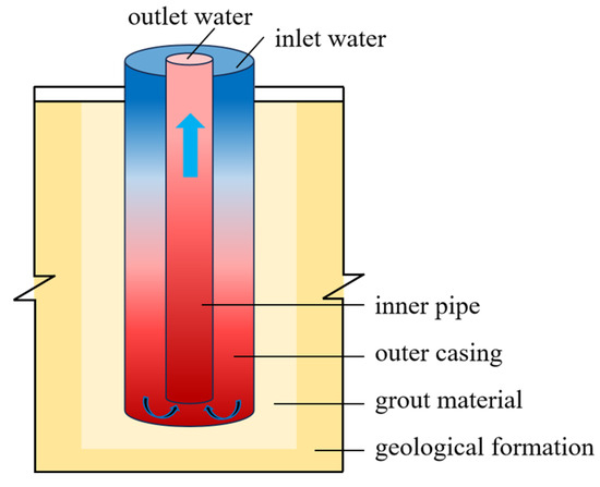
Figure 2.
Structure diagram of a medium-deep buried pipe.
Table 2.
Structural parameters and thermal properties of the MDBHE.
The heat transfer process between the inner and outer pipe water flows can be mathematically characterized by Equation (15).
The equation defines Tp,i and Tp,o as the water temperatures (°C) in the inner and outer pipes, respectively, where ui is the inner pipe flow velocity (m/s), ρw is the water density (kg/m3), Cp,w is the isobaric specific heat capacity of water (kJ/kg·K), Fw,i is the inner pipe’s cross-sectional area (m2), Δt is the time step (s), z is the depth coordinate (m), and Kp,i is the inner pipe’s unit-length thermal conductivity (W/(m2·K)) calculated using Equation (16).
The equation parameters include di,1 as the inner pipe’s internal diameter (m), di,2 as its external diameter (m), λi as the thermal conductivity of the inner pipe material (W/(m·K)), hi,1 as the heat transfer coefficient at the inner pipe’s interior surface, and hi,2 at its exterior surface (both in W/(m2·K)).
The heat transfer process between the outer pipe water flow and the grout–soil medium is mathematically modeled using Equation (17).
In the equation, uo represents the flow velocity of the water in the outer pipe (m/s), Ts denotes the surrounding soil temperature (unit: °C), Aw,o is the flow area of the outer pipe (unit: m2), and Kp,o indicates the thermal conductivity per unit length of the outer pipe (W/(m·°C)), the value of which can be determined using Equation (18).
In the equation, do,1 represents the inner diameter of the outer pipe (unit: m); do,2 denotes the outer diameter of the outer pipe (m); ds indicates the borehole diameter of the ground heat exchanger (m); λo stands for the thermal conductivity of the outer pipe (W/(m·K)); λs signifies the thermal conductivity of the soil (W/(m·K)); ho,1 corresponds to the heat transfer coefficient at the inner surface of the outer pipe (W/(m2·K)); ho,2 refers to the heat transfer coefficient at the outer surface of the outer pipe (W/(m2·K)); and R represents the contact thermal resistance between the ground heat exchanger and backfill material ((m·K)/W).
The heat transfer process within the soil medium is mathematically described in Equation (19).
In the equation, ρ represents the soil density (kg/m3), and Cs denotes the specific heat capacity of the soil (kJ/(kg·K)).
After clarifying the heat exchange relationships among the coaxial casing components, the finite volume method (FVM) proposed in the author’s previous study [12] was applied to calculate the heat transfer processes of the MDBHE. Details were depicted in Supplementary Materials S1. Using these simulation methods, the inlet water temperature and ground-side water flow rate serve as input parameters, and then the transient heat transfer process between the MDBHE and outside ground could be analyzed quantitatively, where the ground temperature and water temperatures variation and distribution, as well as the heat extraction capacity of the MDBHE, could be calculated. Moreover, previous research has shown that thermal interference and performance degradation existed in MDBHEs during long-term operation, and the outlet water temperature decreased by about 6 °C after 100 years of operation [24]. This paper focused on the feasibility of a hybrid system of MDBHEs and ASHPs among different cities with different geothermal conditions and space heating demand, and the long-term operation performance has a similar influence trend among those cities. Therefore, this specific influence has not been considered in this paper and will be studied in detail in future research.
2.4. Models of Heat Pump Systems
Figure 3 presents the simulation model configuration for the water-to-water heat pump. The model operates by inputting operational parameters and employing an assumed COP value to iteratively calculate the actual COP through numerical simulation. The computational process continues until the derived actual COP meets predefined error tolerance criteria, at which point the final value is output. In this article, a magnetic bearing variable-speed centrifugal heat pump (MBC-HP) [20] is selected to conduct further analysis.
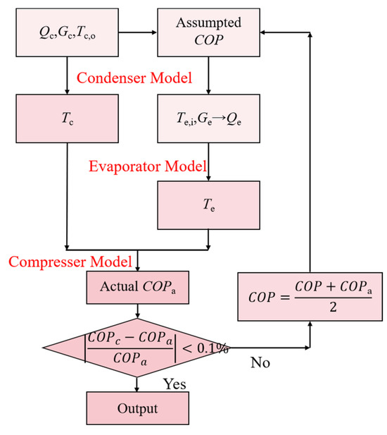
Figure 3.
Simulation model configuration of the heat pump.
Specifically, the COP of heat pumps is determined by the ideal theoretical COP (ICOP) and the compressor efficiency, also named differential COP (DCOP), with Equations (20)–(24).
In this equation, the Tc and Te represent the condensing and evaporating temperatures (K). PLR represents the part load ratio between the practical and rated heating capacity (%). is the condensing and evaporating temperature difference (K). and represent the practical and rated heating capacity of heat pumps (kW). Moreover, the are constant coefficients and are fitted from the field-test results.
It can be seen that the ICOP is determined by the condensing temperature and evaporating temperature, and that there is no correlation with heating capacity. Moreover, the DCOP of the heat pump is determined by the refrigerant flow rate and compression ratio, which can be effectively characterized by the part load ratio (PLR) and the condensing and evaporating temperature difference (Tce). With this simulation mode, the dynamic energy performance of water-to-water heat pumps could be simulated and analyzed quantitatively, under different operation conditions with condenser and evaporator side water temperatures, water flow rates, and the space heating capacity. Furthermore, the detailed calculation methods of the above parameters can be seen in Supplementary Materials S2.
Moreover, the operating performance of ASHPs can be calculated using Equations (25) and (26).
In the equations, COPa,f is the COP of the ASHPs under full-load operating conditions, Tair represents the air temperature (°C), Tc,o,a represents the supply water temperature at the user side of ASHPs (°C), and COPa,p is the practical COP of the ASHPs in actual operating conditions. The PLRa denotes the load ratio of the ASHPs. The coefficients (d1~d6, e1~e3) in the equations are fitted from the data of manufacturers, and details are depicted in Supplementary Materials S3. With this simulation mode, the dynamic energy performance of ASHPs could be simulated and analyzed quantitatively, under different operation conditions with supply water temperatures, air temperatures, and space heating capacities. In summary, the COP of the heat pump unit is primarily influenced by the load ratio, compression ratio, and operating water temperature.
Then, for the gas boilers, the energy efficiency is assumed to be 100%, and the local heat value of gas is used; thus, the gas consumption of gas boilers can be calculated using Equation (27).
In the equation, Ggs is the consumption of natural gas in m3, and Cgs is the calorific value of gas in kJ/m3.
2.5. Control Strategies for Coupled Model Systems
For the system integration configurations mentioned above, the following control logic is established and shown in Figure 4, with the simultaneous minimization of the MDBHE’s investment:
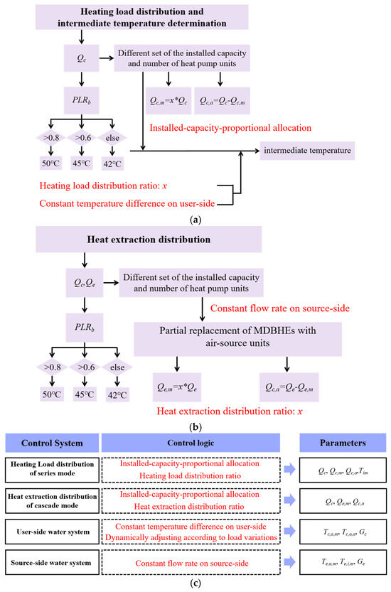
Figure 4.
Control strategies for coupled model systems: (a) Heating load distribution logic of the series mode; (b) Heat extraction distribution logic of the cascade mode; (c) Control logic of the series and cascade modes.
- (1)
- Figure 4a shows the load distribution logic of MD-GHPs and ASHPs for the series mode. The installed capacity and quantities of MD-GHPs and ASHPs are set by the heating load in different cities. Then, during the whole heating season, the transient space heating load is divided between the MD-GHPs (Qc,m) and the ASHPs (Qc,a) according to the same ratio as their installation capacity. Moreover, with the fixed user-side supply and return water temperature difference, the intermediate temperature (Tim) and the outlet water temperatures of the ASHPs (Tc,o,a) are determined by the load distribution ratio.
- (2)
- Figure 4b shows the heat extraction capacity distribution logic of MDBHEs and ASHPs for the cascade mode. The installed heating capacity of water-to-water heat pumps equals the designed maximum heating demand. Different from series mode, the hybrid system in cascade mode primarily allocates the evaporator-side heat extraction capacity of water-to-water heat pumps to the MDBHEs and ASHPs with a specific ratio. Then, the condenser-side inlet and outlet water temperatures of ASHPs remain the same as the values of the MDBHEs.
- (3)
- Figure 4c shows the control logic of the series and cascade modes. User-side supply water temperature varies with heating demand. The temperature is 50 °C when the load ratio (PLR) is greater than 0.8, 45 °C when PLR is between 0.6 and 0.8, and 42 °C otherwise. Then, the supply and return water temperature difference is fixed at 5 °C for the user side, and the water flow rate is fixed at 30m3/h per MDBHE for the ground side. During combined operation, the heating load or the heat extraction capacity is shared between the MD-GHPs and the ASHPs at a specific ratio.
3. Results and Interpretation
3.1. Analysis of Typical Regions
3.1.1. Analysis of Heat Demand in Different Regions
Outdoor temperatures can be obtained from historical meteorological data. Based on the limits for cumulative heating consumption during the heating season in residential buildings across climate zones specified in the national standard GB/T 51161-2016 Civil Building Energy Consumption Standards [25], combined with the heating degree days (HDDs) of different cities, hourly outdoor temperatures and heating loads during the heating season can be determined. The heating season durations are 183 days for severe cold regions and 121 days for both cold regions and hot summer and cold winter regions.
Based on a floor area of 100,000 m2 and the results from Figure 5, the regional peak and per-unit-area load indicators are derived and summarized in Table 3.
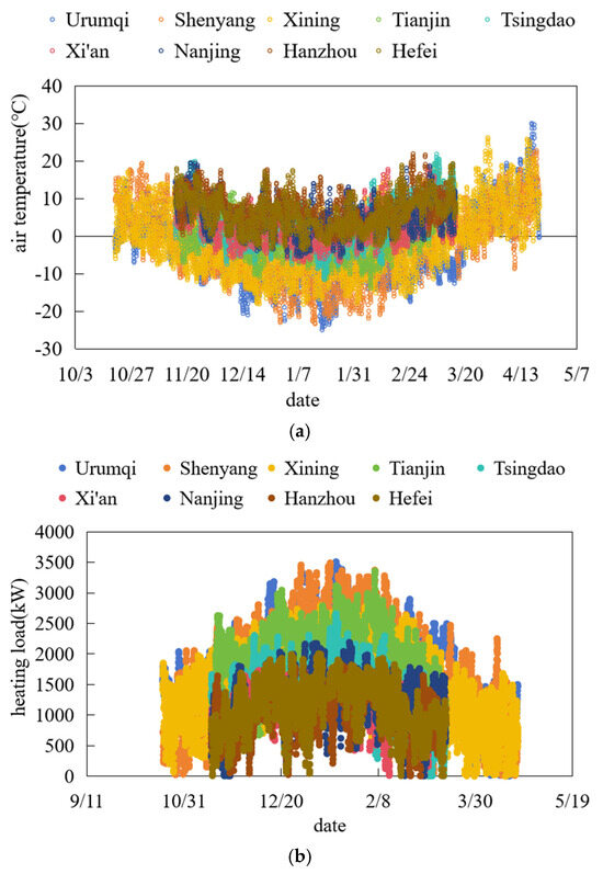
Figure 5.
Hourly air temperature and heating load during the heating season in different regions: (a) Hourly air temperature; (b) Hourly heat load.
Table 3.
Heat load index in major cities across different climate zones.
3.1.2. Analysis of Geothermal Resource Endowment in Different Regions
The geothermal resource endowment across regions is illustrated in Figure 6a, with shading intensity representing heat flow density. It is evident that the Xining region exhibits favorable geothermal resource conditions and efficient ground heat exchange performance. The unit cost of MDBHEs in each region is estimated based on local geological conditions, geothermal resource endowment, and prior engineering experience, as shown in Figure 6b. From the perspectives of the geothermal gradient and rock thermal conductivity, cities exhibit significant differences in heat extraction capacity when adopting medium-deep borehole heat exchangers for heating. A higher geothermal gradient indicates elevated rock temperatures, which creates a greater temperature driving force for heat exchange with the circulating water in the pipes, enhancing efficiency. Similarly, higher rock thermal conductivity reduces thermal resistance during heat transfer, further improving performance.
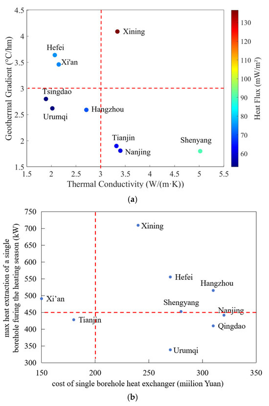
Figure 6.
Cost and cumulative heat extraction of a single borehole heat exchanger in major cities across different climate zones: (a) Thermal properties of soil; (b) Cost and cumulative heat extraction of a single borehole heat exchanger.
Considering both factors, Xining and Lhasa demonstrate high geothermal gradients and rock thermal conductivity, making them highly suitable for developing medium-deep borehole heat pump systems. Conversely, Hohhot, Urumqi, Tsingdao, Changsha, Chengdu, Shanghai, and Hangzhou show poor performance in both metrics, resulting in limited heat exchange capacity and unsuitability for such systems. In summary, this project selects three cities from each of the three climate zones based on their suitability for medium-deep borehole heat pump development for analysis: Urumqi, Shenyang, Xining, Tianjin, Tsingdao, Xi’an, Nanjing, Hangzhou, and Hefei.
3.1.3. Configuration of Medium-Deep Borehole Heat Pump Systems
Based on the geothermal resource endowment and geological condition variations outlined in Section 3.1.2, combined with heating season load demands, the configuration of MD-GHPs for each region includes the number of boreholes and installed capacity. In this study, all regions are configured with 2 units of medium-deep borehole heat pumps, as illustrated in Figure 7. The technical specifications of the heat pump are presented in Table 4 [20].
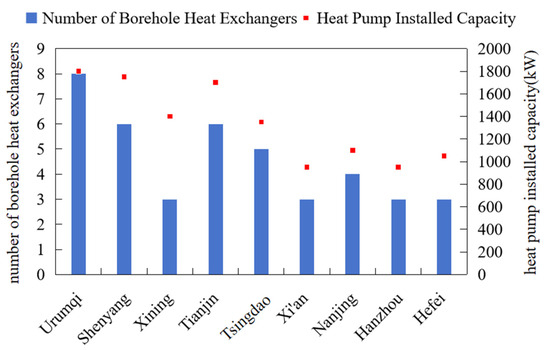
Figure 7.
Number of borehole heat exchangers and heat pump installed capacity in different regions.
Table 4.
The technical specifications of the MD-GHPs [20].
For calculating energy-saving and emission-reduction benefits, the 2022 carbon emission factor for electricity in China [26] is adopted. The primary energy equivalent consumption is calculated using the conversion ratios of 1 kWh of electricity equal to 0.31 kgce and 1 m3 of natural gas equal to 1.33 kgce. Data on electricity prices, carbon emission factors for selected cities, and provincial gas prices are summarized in Figure 8.
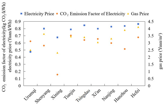
Figure 8.
Electricity price, CO2 emission factor of electricity, and natural gas price in major cities across different climate zones.
3.2. Analysis on Heating Performance and Economic Benefits of MD-GHPs
3.2.1. Heat Exchange Performance of MD-GHPs During the Heating Season
The space heating performance of MD-GHPs in severe cold regions is shown in Figure 9. For Urumqi, the cumulative heat supply during the heating season is 8084.92 MWh, with a peak load of 3508.35 kW, cumulative heat extraction of 6885.12 MWh, and maximum heat extraction of 2707.61 kW. For Shenyang, the cumulative heat supply is 7507.78 MWh, peak load 3490.28 kW, cumulative heat extraction 6413.97 MWh, and maximum heat extraction 2714.60 kW. For Xining, the cumulative heat supply is 6683.53 MWh, peak load 2793.23 kW, cumulative heat extraction 5736.69 MWh, and maximum heat extraction 2128.02 kW. The user-side supply water temperature is determined based on load rate, with a fixed 5 °C temperature difference for the return water. The average source-side water temperatures are 19.06 °C and 13.03 °C for Urumqi, 20.12 °C and 13.14 °C for Shenyang, and 28.44 °C and 15.94 °C for Xining. The source-side circulating water temperature shows an initial decline followed by a rise during the heating season, with the temperature difference first increasing and then decreasing, corresponding to the heating load trend of increasing initially and decreasing afterward.
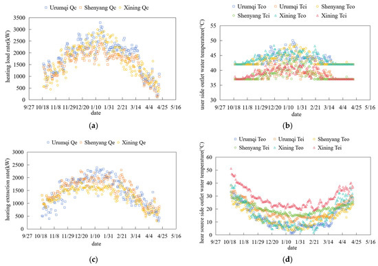
Figure 9.
Space heating performance of MD-GHPs in severe cold region: (a) hourly space heating demand; (b) user-side water temperature; (c) heat extraction rate of MDBHEs; (d) water temperature of MDBHEs.
The space heating performance of MD-GHPs in cold regions is shown in Figure 10. During the heating season, Tianjin achieved a cumulative heat supply of 5556.17 MWh with a peak load of 3359.86 kW, a cumulative heat extraction of 4745.36 MWh, and a maximum heat extraction of 2568.05 kW. Tsingdao recorded a cumulative heat supply of 3894.08 MWh, peak load of 2668.16 kW, cumulative heat extraction of 3383.44 MWh, and maximum heat extraction of 2048.93 kW. Xi’an reported a cumulative heat supply of 3333.43 MWh, peak load of 1831.69 kW, cumulative heat extraction of 2904.66 MWh, and maximum heat extraction of 1472.52 kW. The user-side supply water temperature varies with load rate, while the return water temperature maintains a fixed 5 °C temperature difference. Average source-side water temperatures are 19.32 °C and 11.50 °C for Tianjin, 23.21 °C and 16.52 °C for Tsingdao, and 26.09 °C and 16.52 °C for Xi’an. The source-side circulating water temperature first decreases and then increases during the heating season, with the temperature difference initially expanding and later contracting, mirroring the heating load trend of rising followed by declining demand.
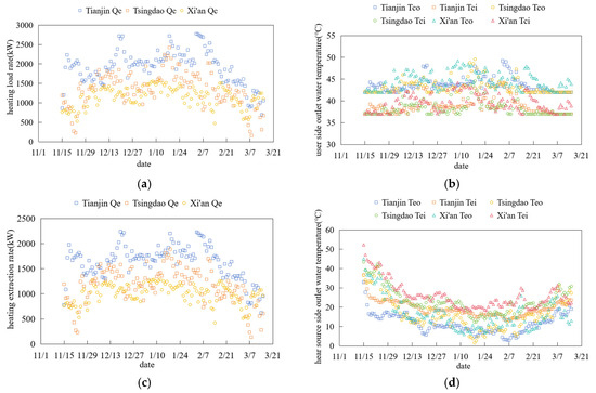
Figure 10.
Space heating performance of MD-GHPs in cold region: (a) hourly space heating demand; (b) user-side water temperature; (c) heat extraction rate of MDBHEs; (d) water temperature of MDBHEs.
The heat exchange performance of MDBHEs in hot summer and cold winter regions is illustrated in Figure 11. During the heating season, Nanjing achieved a cumulative heat supply of 3567.57 MWh with a peak load of 2190.05 kW, cumulative heat extraction of 3085.64 MWh, and maximum heat extraction of 1766.18 kW. Hangzhou recorded a cumulative heat supply of 2977.20 MWh, peak load of 1893.10 kW, cumulative heat extraction of 2599.41 MWh, and maximum heat extraction of 1545.74 kW. Hefei reported a cumulative heat supply of 3354.24 MWh, peak load of 2004.46 kW, cumulative heat extraction of 2935.13 MWh, and maximum heat extraction of 1666.18 kW. The user-side supply water temperature varies according to load rate, while the return water temperature maintains a fixed 5 °C temperature difference. Average source-side water temperatures are 21.90 °C and 14.28 °C for Nanjing, 26.54 °C and 17.97 °C for Hangzhou, and 28.79 °C and 19.52 °C for Hefei. The source-side circulating water temperature exhibits an initial decrease followed by an increase during the heating season, accompanied by a temperature difference that first expands and then contracts, aligning with the heating load trend of rising and subsequently decreasing demand.
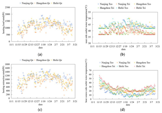
Figure 11.
Space heating performance of MD-GHPs in hot summer and cold winter region: (a) hourly space heating demand; (b) user-side water temperature; (c) heat extraction rate of MDBHEs; (d) water temperature of MDBHEs.
3.2.2. Energy Performance of MD-GHPs During the Heating Season
The energy performance of MD-GHPs during heating seasons is shown in Figure 12. Overall efficiency remains high, though system performance declines during extreme cold periods due to reduced ground-side circulating water temperatures and increased load-side heating demands. Key metrics include the following: Urumqi achieves a unit COP of 6.74 and system COPs of 5.31, Shenyang records 6.86 and 4.43, Xining maintains 7.06 and 5.50, Tianjin shows 6.85 and 5.38, Tsingdao demonstrates 7.63 and 5.84, Xi’an reaches 7.77 and 5.93, Nanjing attains 7.40 and 5.71, Hangzhou achieves 7.88 and 5.99, and Hefei leads with 8.00 and 6.06. Cold regions and hot summer and cold winter zones exhibit superior energy efficiency, highlighting the significant potential of MD-GHPs in the northern and select southern areas of China. Additional technical indicators, economic benefits, and carbon reduction data are detailed in Table 5.
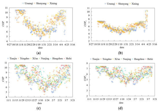
Figure 12.
Energy performance of MD-GHPs in different regions: (a) COP of heat pumps in severe cold region; (b) COPs of MD-GHPs in severe cold region; (c) COP of heat pumps in cold region and hot summer and cold region; (d) COPs of MD-GHPs in cold region and hot summer and cold region.
Table 5.
System performance of medium-deep borehole heat pump systems during the heating season in different regions.
3.3. Analysis on Operational Performance and Economic Benefits of Different Heat Source Systems
Based on the previously calculated peak loads for each region, the installed capacities of air-source heat pumps and gas boilers can be determined, and their corresponding initial investments are calculated. Specific configurations are detailed in Table 6.
Table 6.
System configuration of air-source heat pump and gas-fired boiler.
The performance of air-source heat pumps during heating seasons across regions is illustrated in Figure 13. As ASHPs extract heat directly from outdoor air, their evaporation temperatures decrease with declining ambient air temperatures. Concurrently, rising building heating demands drive higher supply water temperatures and elevated condensation temperatures on the condenser side, resulting in a distinct trend of initially decreasing and later recovering COPs throughout the heating season. Key performance metrics are as follows: Urumqi achieves a unit COP of 2.69 and system COPs of 2.43, Shenyang records 2.77 and 2.50, Xining maintains 2.81 and 2.66, Tianjin shows 2.97 and 2.81, Tsingdao demonstrates 3.16 and 2.97, Xi’an reaches 3.09 and 2.91, Nanjing attains 3.28 and 3.08, Hangzhou achieves 3.42 and 3.20, and Hefei registers 3.28 and 3.08. Hot summer and cold winter zones exhibit higher air-source heat pump efficiency compared to severe cold and cold regions due to their relatively milder winter temperatures.
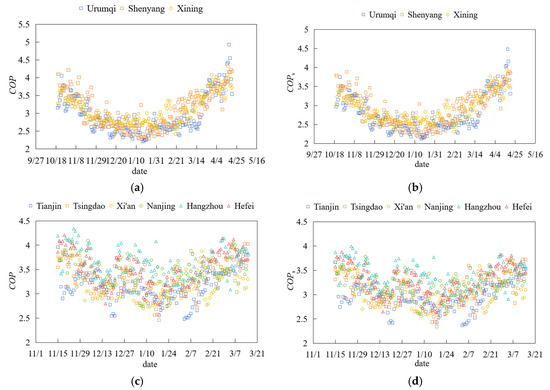
Figure 13.
Energy performance of ASHPs in different regions: (a) COP of heat pumps in severe cold region; (b) COPs of ASHPs in severe cold region; (c) COP of heat pumps in cold region and hot summer and cold region; (d) COPs of ASHPs in cold region and hot summer and cold region.
The energy consumption of the gas-fired boiler system was calculated directly using data from Section 2.4. The energy consumption of the three heat source systems was converted into standard coal equivalent. Combined with the cumulative heat supply (GJ), the energy consumption, carbon emissions, and operating costs per unit heat supplied for each system were calculated. The results are presented in Figure 14. As shown in the figure, the MD-GHPs demonstrate significant advantages in energy consumption, carbon emissions, and annual operating costs due to their high energy efficiency. Compared to the ASHPs, the MD-GHPs achieve energy-saving rates ranging from 43.67% to 54.29%, operating cost reductions of 43.67% to 54.29%, and carbon emission reductions from 43.67% to 54.29%. In contrast, compared to the gas-fired boiler, the MD-GHPs exhibit energy-saving rates from 50.08% to 63.52%, operating cost reductions from 50.04% to 66.90%, and carbon emission reductions from 9.41% to 91.80%.
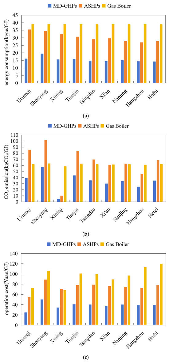
Figure 14.
Energy consumption, carbon emissions, and cost per unit heat supply of single heat source heat pump systems: (a) Energy consumption per unit heat supply for different heat source systems; (b) CO2 emission per unit heat supply for different heat source systems; (c) Cost per unit heat supply for different heat source systems.
The total costs of different heat source systems over 25 years in each city were statistically analyzed, as shown in Figure 15. The adaptability of the three heat source systems varies across cities. In some cities, MD-GHPs demonstrate favorable economic benefits within relatively short payback periods. For example, in Xining and Xi’an, the incremental payback periods of the MD-GHPs compared to the gas-fired boiler are 9 years and 7 years, respectively, and both are 7 years compared to the ASHPs. Conversely, in cities such as Urumqi, Tsingdao, and Hangzhou, the ASHPs consistently exhibit the best economic performance over extended periods, with incremental payback periods for the MD-GHPs reaching 23 to 26 years in these regions.
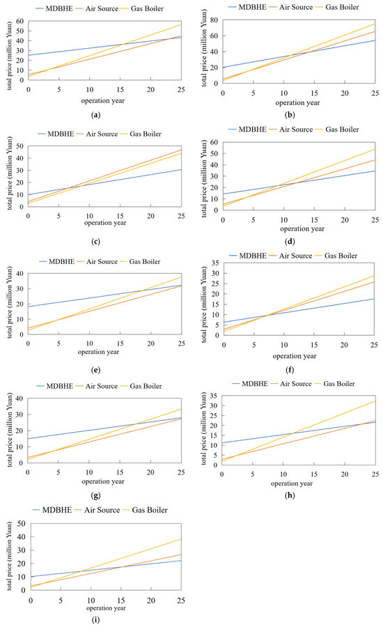
Figure 15.
Operating costs of different heat source systems in different regions over 25 years: (a) Urumqi; (b) Shenyang; (c) Xining; (d) Tianjin; (e) Tsingdao; (f) Xi’an; (g) Nanjing; (h) Hangzhou; (i) Hefei.
In summary, the MD-GHPs exhibit higher energy efficiency and demonstrate significant advantages during operation, characterized by lower operational energy consumption and costs. However, due to geological constraints, limited geothermal resource availability, and high drilling costs, the initial investment for MD-GHP systems is substantially elevated, hindering their widespread adoption. In contrast, ASHPs require lower upfront costs, as their initial investment primarily covers the heat pump unit themself. Yet, challenges such as frost accumulation during winter significantly reduce its heating-season efficiency, leading to higher energy consumption and operational costs, which diminish their long-term economic viability. These findings highlight the rationale and necessity of hybrid systems combining multiple heat sources, which balance upfront costs, operational efficiency, and long-term sustainability to optimize overall performance.
4. Discussion
4.1. Performance Analysis of Different Combination Modes
This section conducts an analysis of system energy efficiency and economic benefits under different coupling modes using Urumqi as a case study, aiming to identify the optimal hybrid configuration.
4.1.1. Typical Operating Condition Single-Point Performance Analysis
Figure 16 illustrates the single-point performance of the system under series mode. Under these conditions, the user-side supply and return water temperatures are 50 °C and 45 °C, respectively, with a total flow rate of 566.36 m3/h. For the borehole side, the inlet and outlet temperatures are 1.15 °C and 10.28 °C, respectively, utilizing four boreholes and a single-hole flow rate of 30 m3/h. The total user-side heat supply is 3288.06 kW, equally contributed by the MD-GHPs and ASHPs at 1644.03 kW each. Power consumption includes 372.15 kW for the MD-GHPs, 747.82 kW for the ASHPs, 32.88 kW for the borehole-side pump, and 65.76 kW for the user-side pump. Calculated COP are as follows: MD-GHPs achieve a unit COP (COPm) of 4.42 and a system COPs (COPs,m) of 3.75, while ASHPs yield a unit COP (COPa) of 2.20 and a system COPs (COPs,a) of 2.10, resulting in an integrated system COPs (COPs) of 2.70 for the series configuration. From a heat flow perspective, the thermal energy extracted by both heat pumps, combined with their electrical input, collectively supplies heat to the user side.
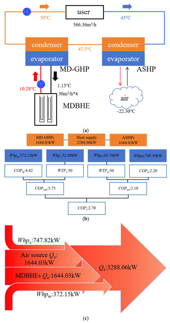
Figure 16.
Typical operating condition of series mode system: (a) Single-point parameters of series mode system; (b) Single-point performance of series mode system; (c) Energy flow of the series mode system.
Figure 17 illustrates the single-point performance of the system under cascade mode. Under these conditions, the user-side supply and return water temperatures are 50 °C and 45 °C, respectively, with a total flow rate of 566.36 m3/h. For the evaporation side, the inlet and outlet temperatures are 10.28 °C and 1.15 °C, respectively, with a total source-side flow rate of 240 m3/h (including 120 m3/h for the ASHPs and a single-borehole flow rate of 30 m3/h for the MDBHEs). The total user-side heat supply is 3288.06 kW, with a total source-side heat extraction of 2543.76 kW, equally contributed by the MDBHEs and ASHPs at 1644.03 kW each. Power consumption includes 744.30 kW for the water-to-water heat pump, 349.54 kW for the ASHPs, 65.76 kW for the source-side pump, and 65.76 kW for the user-side pump. Calculated COP are as follows: the water-to-water heat pump achieves a unit COP (COPm) of 4.42 and a system COPs (COPs,m) of 3.75, while the ASHPs yield a unit COP (COPa) of 2.22, resulting in an integrated system COPs (COPs) of 2.70 for the cascade configuration. From a heat flow perspective, the thermal energy extracted by both heat pumps, combined with their electrical input, collectively supplies heat to the user side, similar to the series mode.
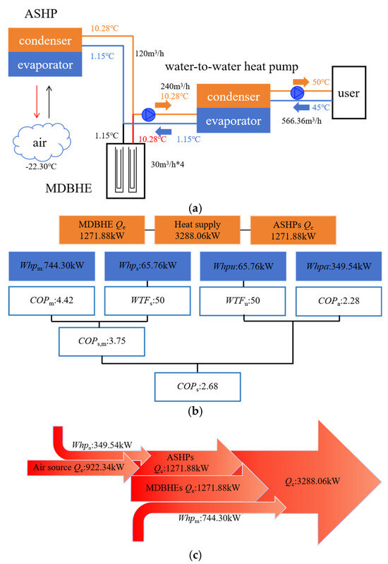
Figure 17.
Typical operating conditions of cascade mode system: (a) Single-point parameters of cascade mode system; (b) Single-point performance of cascade mode system; (c) Energy flow of cascade mode system.
The results from Figure 16 and Figure 17 allow for a theoretical comparison to determine the optimal coupling configuration. The series mode demonstrates superior overall performance across the entire heating season. This is because the ASHPs in series mode only need to supply water at an intermediate temperature, which is generally lower than the ASHPs’ supply temperature in pure ASHPs. Consequently, the lower condensing temperature in series mode enhances ASHPs’ efficiency throughout the heating season.
In cascade mode, the ASHPs operate with even lower supply water temperatures and condensing temperatures compared to the series mode, theoretically improving their efficiency (as shown in Equation (28)). However, despite this advantage, the cascade system’s overall efficiency is reduced due to the additional pump power consumption on the source side. Specifically, the water-to-water heat pump in cascade mode requires the same installed capacity as the standalone MD-GHPs system; however, the source-side pump power increases significantly compared to the series mode. This results in a lower integrated system COPs for the cascade configuration (as calculated using Equation (29)).
In the equations, COPa denotes the unit energy efficiency of the ASHPs, and COPs represents the integrated energy efficiency of the hybrid system. Here, Qc is the total user-side heat supply (kW), Whpa is the power consumption of the ASHPs (kW), Whpm is the power consumption of the water-to-water heat pump (kW), and Whpu and Whps are the power consumptions of the user-side and source-side pumps (kW), respectively; all power values are expressed in kW. The calculated results yield COPa = 2.28 and COPs = 2.68.
4.1.2. Comparison of Performance of Different Combination Modes
Figure 18 and Figure 19 present the system performance of two coupling modes throughout the heating season, all operating with a 50% load distribution ratio. The number of MDBHEs is 4 units, half of the pure MD-GHP systems. During the entire heating period, the average air temperature (Tair), representing the mean inlet air temperature of the ASHPs, measures −4.48 °C. The average supply and return water temperatures at the user side (Tc,o, Tc,i) are recorded as 43.55 °C and 38.55 °C, respectively. The series mode demonstrates an average intermediate temperature (Tim) of 41.05 °C, while the ground heat exchanger side maintains mean inlet and outlet circulating water temperatures (Te,o,m, Te,i,m) of 13.43 °C and 19.06 °C, respectively.
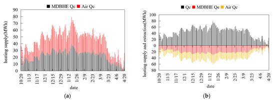
Figure 18.
Composition of the heat supply of different modes: (a) Series mode systems; (b) Cascade mode systems.
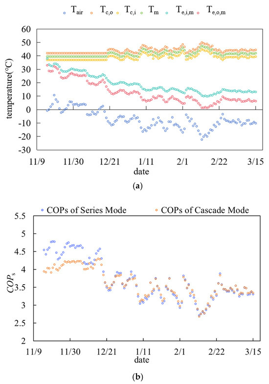
Figure 19.
Operating performance of different modes: (a) Temperature of condenser and evaporator of different modes; (b) COPs of different modes.
Under identical load distribution ratios, the series mode exhibits equivalent cumulative heat supply from medium-deep and air-source systems, reaching 4042.5 MWh. In the cascade mode, the water-to-water heat pump delivers a heat supply identical to that of the pure MD-GHPs system (8084.9 MWh), while the ASHPs provide 3442.6 MWh to the source side of the water-to-water heat pump. The total electricity consumption is quantified as 2294.5 MWh for the series mode (MD-GHPs: 761.5 MWh; ASHPs: 1533.0 MWh), achieving an efficiency of 3.52 and 2309.1 MWh for the cascade mode (MD-GHPs: 1523.2 MWh; ASHPs: 785.9 MWh), yielding an efficiency of 3.50. A comparative analysis of seasonal energy efficiency confirms the superior performance of the series mode.
4.1.3. Comparison of Economic Benefits of Different Combination Modes
Figure 20 illustrates the economic costs of different heat source systems and coupling configurations over a 25-year period. The pure ASHP system demonstrates favorable economic performance within the first 20 years due to its lower initial investment, though its higher energy consumption results in elevated operational expenses and rapid cumulative cost escalation. Conversely, the pure MD-GHP system requires substantial upfront capital but exhibits lower energy demand and reduced annual operational costs, leading to gradual cost growth. The two coupling modes occupy an intermediate position, featuring lower initial investments than the pure MD-GHPs system while maintaining operational expenses below those of the pure ASHPs configuration. At the 15th and 20th year marks, the pure ASHP system remains economically advantageous. However, by the 25th year, the series-coupled mode emerges as the most cost-effective solution. This temporal evolution of economic viability suggests that the pure ASHPs represent the optimal choice for Urumqi under the evaluated conditions.
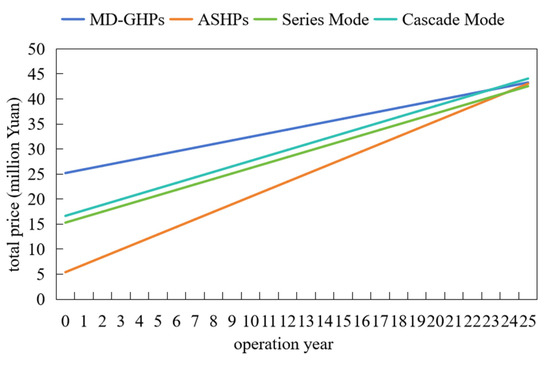
Figure 20.
Comparative analysis of economic benefits for heat pump systems with different heat sources in Urumqi.
4.2. Adaptability Analysis of Series Mode Systems in Different Climate Zones
Section 4.1 has established the technical superiority of the series-coupled mode through operational principles and seasonal performance analysis. This section evaluates its economic viability by investigating system configurations, specifically analyzing the impact of ground heat exchanger quantities. As revealed in Section 4.1.3, the high-efficiency and low-energy-consumption advantages of MD-GHPs fail to offset their capital costs in Urumqi due to the region’s exceptionally low electricity rates, rendering the pure ASHP system more economically favorable. To better assess the configuration adaptability of the series-coupled mode, this study shifts its geographic focus to Shenyang, where energy market conditions differ substantially. The analysis specifically examines how varying numbers of MDBHEs (4, 6, and 8 units) influence the economic performance of series-coupled systems in this distinct operational context.
As shown in Figure 21, the pure ASHP system (0 MDBHEs) requires an initial investment of 5.4 million yuan, with annual electricity consumption of 2857.78 MWh and operational costs of 2.29 million yuan based on the local electricity rate of 0.8 yuan/kWh. Configurations with incremental MDBHEs exhibit progressively higher initial investments and lower operational costs: 1 unit (7.9 million yuan initial, 2588.31 MWh consumption, 2.07 million yuan annual cost), 2 units (10.4 million yuan, 2328.97 MWh, 1.86 million yuan), 3 units (12.9 million yuan, 2079.98 MWh, 1.66 million yuan), 4 units (15.4 million yuan, 1842.20 MWh, 1.47 million yuan), 5 units (17.9 million yuan, 1619.06 MWh, 1.30 million yuan), and the pure MD-GHPs system with 6 units (20.3 million yuan, 1394.12 MWh, 1.12 million yuan). The analysis confirms the air-source system as the most economical option within 5–10 years, while the pure MD-GHP achieves optimal cost-effectiveness from the 15th year onward.
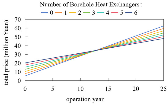
Figure 21.
Economic benefit analysis of series mode systems with different borehole heat exchanger configurations in Shenyang.
Figure 22 demonstrates the regional adaptability and economic performance of different series system configurations. Similar to single-source heating systems, the pure medium-deep and pure ASHP systems maintain strong economic advantages in multiple regions within specific operational periods. In Xining, the ASHPs prove optimal within the first 6 years, while the pure MD-GHPs system becomes cost-effective from the seventh year onward. For Xi’an, the ASHPs system dominates for the initial 7 years, with the pure MD-GHPs configuration taking precedence starting from the eighth year. Nanjing retains the pure ASHP system as the most economical option until the 23rd year. Cities such as Tianjin and Hefei exhibit prolonged dominance of the ASHP system, transitioning to the pure MD-GHP system only at the 14th and 19th years, respectively, with Hefei showing temporary superiority of the series mode between 13 and 16 years. The series mode achieves economic prominence primarily during the 20–25-year operational period in regions like Urumqi, Tsingdao, and Hangzhou, where the ASHP systems remain optimal for the first 20 years. Specifically, the series configuration becomes cost-effective in Urumqi and Tsingdao at the 24th year, and in Hangzhou at the 22nd year.
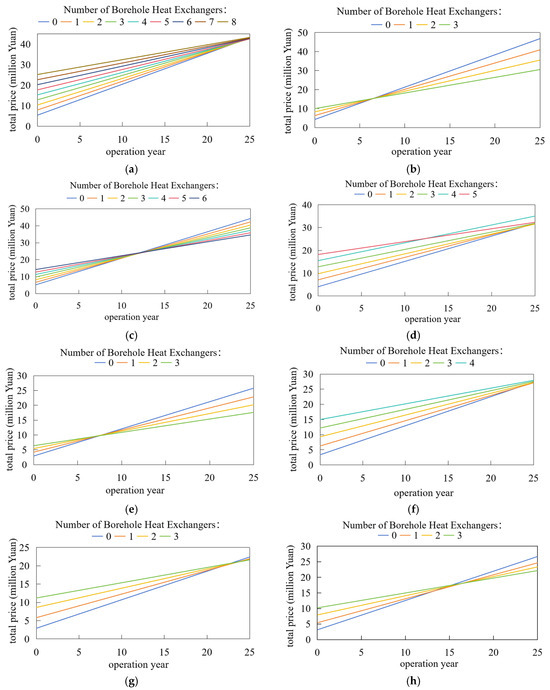
Figure 22.
Operating costs of different heat source systems in different regions over 25 years: (a) Urumqi; (b) Xining; (c) Tianjin; (d) Tsingdao; (e) Xi’an; (f) Nanjing; (g) Hangzhou; (h) Hefei.
5. Conclusions
This study proposes a novel hybrid system integrating MD-GHPs and ASHPs configurations. Through numerical simulations and controlled variable analysis, the adaptability of this coupled system across diverse regions and its optimal configuration are systematically investigated. Key findings indicate that the hybrid system effectively balances energy efficiency, economic feasibility, and regional adaptability by leveraging the complementary advantages of both heat sources. The conclusions are as follows:
- The series-coupled mode demonstrates superior performance among the three hybrid configurations. By implementing intermediate temperature control, it reduces the user-side supply water temperature of the ASHPs during heating seasons, thereby lowering condensation temperatures. Compared to cascade systems, it achieves lower source-side pump energy consumption and higher seasonal energy efficiency, with a COP of 3.52 in Urumqi. Its advantages in energy allocation optimization and thermal regulation establish it as the optimal integration strategy for MD-GHP and ASHP systems.
- Regional adaptability of heat source configurations depends on geothermal resource endowment, climatic conditions, and electricity price dynamics. Cities with abundant geothermal resources and favorable geology (e.g., Xining, Xi’an) favor pure MD-GHPs systems, while regions with limited geothermal potential and challenging geology (e.g., Tsingdao, Hangzhou) show better suitability for pure ASHPs systems. Intermediate-resource areas require customized configurations balancing operational demands and energy market fluctuations.
- The hybrid system synergistically combines the advantages of both heat sources, offering relatively low initial investments and operational costs. However, economic superiority varies temporally across cities due to electricity price influences: the series mode configuration generally achieves optimal cost–benefit equilibrium between initial and operational expenses during the 20th–25th operational years, as exemplified by Urumqi, Tsingdao, and Hefei, where it effectively balances capital expenditures with long-term energy savings.
Supplementary Materials
The following supporting information can be downloaded at: https://www.mdpi.com/article/10.3390/buildings15111938/s1, Figure S1.1: Meshes discretization of MDBHE and surrounding ground; Figure S1.2: The ground temperature distribution at the depth of 2530–2700 m; Figure S1.3: The ground temperature distribution in radius direction at the bottom of MDBHEs; Figure S2.1: Simulation Model Configuration of the Heat Pump; Figure S3.1: COP of ASHPs under different operation conditions; Table S1.1: The physical dimension and thermo-physical property of the soil and rocks; Table S1.2: Mesh independence analysis; Table S2.1: Design parameters of the heat pump; Table S2.2: Regression values of constant coefficients; Table S3.1: Regression values of constant coefficients of ASHPs.
Author Contributions
Conceptualization, Simulation, Writing—Original Draft, Y.W.; Methodology, Supervision, Funding acquisition, J.D.; Methodology, Y.S.; Simulation, C.P.; Field Tests, M.M.; Field Tests, Y.C.; Data Curation, L.F.; Data Curation, M.C.; Supervision, Q.W.; Supervision, H.Z. All authors have read and agreed to the published version of the manuscript.
Funding
This research was funded by the National Natural Science Foundation of China (Grant No. 52308095) and the Natural Science Foundation of Hubei Province of China (Grant No. 2024AFB586).
Data Availability Statement
Data are contained within the article.
Conflicts of Interest
The authors declare no conflicts of interest.
References
- Nie, Y.Z.; Deng, M.S.; Shan, M.; Yang, X.D. Clean and low-carbon heating in the building sector of China: 10-Year development review and policy implications. Energy Policy 2023, 179, 113659. [Google Scholar] [CrossRef]
- Yuan, M.; Mathiesen, B.V.; Schneider, N.; Xia, J.; Zheng, W.; Sorknæs, P.; Lund, H.; Zhang, L. Renewable energy and waste heat recovery in district heating systems in China: A systematic review. Energy 2024, 294, 130788. [Google Scholar] [CrossRef]
- Cui, P.; Yang, W.; Zhang, W.; Zhu, K.; Spitler, J.D.; Yu, M. Advances in ground heat exchangers for space heating and cooling: Review and perspectives. Energy Built Environ. 2024, 5, 255–269. [Google Scholar] [CrossRef]
- Deng, J.; Wei, Q.; He, S.; Liang, M.; Zhang, H. What is the main difference between medium-depth geothermal heat pump systems and conventional shallow-depth geothermal heat pump systems? Field tests and comparative study. Appl. Sci. 2019, 9, 5120. [Google Scholar] [CrossRef]
- Deng, J.; Ma, M.; Wei, Q.; Liu, J.; Zhang, H.; Li, M. A specially-designed test platform and method to study the operation performance of medium-depth geothermal heat pump systems (MD-GHPs) in newly-constructed project. Energy Build. 2022, 272, 112369. [Google Scholar] [CrossRef]
- Yishuo, X.; Yukun, S.; Sumin, Z. Heat extraction by deep coaxial borehole heat exchanger for clean space heating near Beijing, China: Field test, model comparison and operation pattern evaluation. Renew. Energy 2022, 199, 803–815. [Google Scholar]
- Wang, Z.; Wang, F.; Liu, J.; Ma, Z.; Han, E.; Song, M. Field test and numerical investigation on the heat transfer characteristics and optimal design of the heat exchangers of a deep borehole ground source heat pump system. Energy Convers. Manag. 2017, 153, 603–615. [Google Scholar] [CrossRef]
- Holmberg, H.; Acuna, J.; Næss, E.; Sønju, O.K. Thermal evaluation of coaxial deep borehole heat exchangers. Renew. Energy 2016, 97, 65–76. [Google Scholar] [CrossRef]
- Beier, R.A.; Fossa, M.; Morchio, S. Models of thermal response tests on deep coaxial borehole heat exchangers through multiple ground layers. Appl. Therm. Eng. 2021, 184, 116241. [Google Scholar] [CrossRef]
- Moreira, D.; Macias, J.; Hidalgo-Leon, R.; Jervis, F.X.; Soriano, G. Performance of a borehole heat exchanger: The influence of thermal properties estimation under tidal fluctuation. Eng. Sci. Technol. Int. J. 2022, 30, 101057. [Google Scholar]
- Beier, R.A. Thermal response tests on deep borehole heat exchangers with geothermal gradient. Appl. Therm. Eng. 2020, 178, 115447. [Google Scholar] [CrossRef]
- Luo, Y.Q.; Cheng, N.; Xu, G.Z. Analytical modeling and thermal analysis of deep coaxial borehole heat exchanger with stratified-seepage-segmented finite line source method (S3-FLS). Energy Build. 2022, 257, 111795. [Google Scholar] [CrossRef]
- Al-Kbodi, B.H.; Rajeh, T.; Li, Y.; Zhao, J.; Zhao, T.; Zayed, M.E. Heat extraction analyses and energy consumption characteristics of novel designs of geothermal borehole heat exchangers with elliptic and oval double U-tube structures. Appl. Therm. Eng. 2023, 235, 121418. [Google Scholar] [CrossRef]
- Lund, A.E.D. Effect of heat and mass transfer related parameters on the performance of deep borehole heat exchangers. Appl. Therm. Eng. 2024, 253, 123764. [Google Scholar] [CrossRef]
- Gola, G.; Sipio, E.D.; Facci, M.; Galgaro, A.; Manzella, A. Geothermal deep closed-loop heat exchangers: A novel technical potential evaluation to answer the power and heat demands. Renew. Energy 2022, 198, 1193–1209. [Google Scholar] [CrossRef]
- Deng, J.; Peng, C.; Su, Y.; Qiang, W.; Cai, W.; Wei, Q. Research on the heat storage characteristic of deep borehole heat exchangers under intermittent operation mode: Simulation analysis and comparative study. Energy 2023, 282, 128938. [Google Scholar] [CrossRef]
- Huang, S.; Zhu, K.; Dong, J.; Li, J.; Kong, W.; Jiang, Y.; Fang, Z. Heat transfer performance of deep borehole heat exchanger with different operation modes. Renew. Energy 2022, 193, 645–656. [Google Scholar] [CrossRef]
- Deng, J.; Peng, C.; Su, Y.; Qiang, W.; Wei, Q. Research on the long-term operation performance of deep borehole heat exchangers array: Thermal attenuation and maximum heat extraction capacity. Energy Build. 2023, 298, 113511. [Google Scholar] [CrossRef]
- Wang, C.; Ma, M.; Su, Y.; Wang, Y.; Wang, Y.; Chen, Y.; Deng, J. Research on the operation features and optimization methods of heat pumps coupled with mid-deep borehole heat exchangers: On-site measurements and comparative study. Energy Build. 2025, 328, 115239. [Google Scholar] [CrossRef]
- Deng, J.; Su, Y.; Peng, C.; Qiang, W.; Cai, W.; Wei, Q.; Zhang, H. How to improve the energy performance of mid-deep geothermal heat pump systems: Optimization of heat pump, system configuration and control strategy. Energy 2023, 285, 129537. [Google Scholar] [CrossRef]
- Wang, Z.; Wang, F.; Liu, J.; Li, Y.; Wang, M.; Luo, Y.; Ma, L.; Zhu, C.; Cai, W. Energy analysis and performance assessment of a hybrid deep borehole heat exchanger heating system with direct heating and coupled heat pump approaches. Energy Convers. Manag. 2023, 276, 116484. [Google Scholar] [CrossRef]
- He, W.; Ren, B.; Jin, H.; Liu, R.; Luo, H.; Luo, Y.; Zhou, C. Geothermal cascade utilization for low-carbon building cooling and heating via collaboration of shallow and deep borehole heat exchanger array. J. Build. Eng. 2025, 101, 111870. [Google Scholar] [CrossRef]
- Li, J.; Bao, L.; Niu, G.; Miao, Z.; Guo, X.; Wang, W. Research on renewable energy coupling system based on medium-deep ground temperature attenuation. Appl. Energy 2024, 353, 122187. [Google Scholar] [CrossRef]
- Deng, J.; Qiang, W.; Peng, C.; Wei, Q.; Cai, W.; Zhang, H. Can deep borehole heat exchangers operate stably in long-term operation? Simulation analysis and design method. J. Build. Eng. 2022, 62, 105358. [Google Scholar] [CrossRef]
- GB/T 51161-2016; Standard for Building Energy Consumption of Urban Buildings. China Architecture & Building Press: Beijing, China, 2016.
- Ministry of Ecology and Environment of the People’s Republic of China. Announcement on Releasing the 2022 Electricity Carbon Dioxide Emission Factors (Annex: 2022 Electricity Carbon Dioxide Emission Factors). Available online: https://www.mee.gov.cn (accessed on 26 December 2024).
Disclaimer/Publisher’s Note: The statements, opinions and data contained in all publications are solely those of the individual author(s) and contributor(s) and not of MDPI and/or the editor(s). MDPI and/or the editor(s) disclaim responsibility for any injury to people or property resulting from any ideas, methods, instructions or products referred to in the content. |
© 2025 by the authors. Licensee MDPI, Basel, Switzerland. This article is an open access article distributed under the terms and conditions of the Creative Commons Attribution (CC BY) license (https://creativecommons.org/licenses/by/4.0/).