Soil Parameter Inversion in Dredger Fill Strata Using GWO-MLSSVR for Deep Foundation Pit Engineering

Abstract

Accurate determination of constitutive model parameters is crucial for reliable numerical simulation in deep foundation pit engineering. This study presents an inverse analysis method using Multioutput Least-Squares Support Vector Regression (MLSSVR) optimized by the Gray Wolf Optimization (GWO) algorithm to invert key parameters of the Hardening Soil (HS) model. A case study on a foundation pit in the dredger fill stratum of Xiamen Railway integrates finite element simulation with machine learning. The proposed GWO-MLSSVR model demonstrates high predictive accuracy, with lateral displacement predictions closely matching field monitoring data and relative errors within 5% at various depths of measurement point. Compared to traditional inversion methods and MLSSVR models optimized by other algorithms, this approach significantly reduces prediction errors. Additionally, the influence of construction stages, input layer nodes, and training sample size on inversion performance is investigated. This method provides a practical and efficient solution for accurately obtaining soil parameters under complex soil conditions, thereby enhancing the reliability of geotechnical numerical simulations and offering valuable guidance for foundation pit design and safety assessment.

1. Introduction

A critical aspect of studying and analyzing deep foundation pit excavation through numerical simulation is the accurate determination of the soil’s constitutive parameters within the excavation zone [1]. Soil is inherently non-homogeneous, nonlinear, and discontinuous [2], making it particularly challenging to accurately characterize its fundamental properties. Existing numerical simulations indicate that the use of conventional constitutive models—such as the Mohr–Coulomb, Cambridge, and Duncan–Chang models—often leads to inaccurate assessments of settlement behind the retaining wall, settlement in remote zones, and the overall extent of influence [3]. As a result, simulation outcomes frequently diverge from field monitoring data. The Hardening Soil (HS) model improves analysis precision by incorporating the stress-dependence of soil stiffness and distinguishing between loading and unloading behaviors [4]. This model has been effectively applied in foundation excavation projects involving dredger fill strata, with multiple engineering practices confirming its reliability and accuracy [5]. However, compared to other models, the HS model includes parameters that are more difficult to determine accurately. These parameters are often obtained from geological reports or empirical formulas, which may be reasonable but do not fully reflect actual soil conditions. When such approximated parameters are used in finite element simulations, the resulting predictions often contain substantial errors [6]. Therefore, the rapid and accurate acquisition of soil constitutive parameters remains a key challenge and focus in current numerical simulation research for deep foundation pit engineering [7].

The advancement of machine learning has expanded the application of intelligent analysis in geotechnical engineering, and the integration of finite element analysis with artificial intelligence has become increasingly common in this field. The combination of machine learning models and advanced optimization algorithms demonstrates significant potential in improving model accuracy and efficiency. For instance, J.J. Zhang et al. [8] applied the alternating direction (AD) method within the Markov Chain Monte Carlo (MCMC) algorithm—widely used in rock physics inversion—to improve the convergence of inversion models. This work established a theoretical relationship between seismic elastic properties and parameters such as porosity, saturation, and clay content. Z.M. Yaseen et al. [9] employed the extreme learning machine (ELM) to evaluate its performance compared to other machine learning models in predicting the compressive strength of foamed concrete. M.N.A. Raja et al. [10] utilized data gathered from validated finite element numerical models as training samples to develop gene expression programming (GEP) models for risk analysis in civil engineering projects. R. Tang et al. [11] proposed an inversion of soft soil foundation parameters using a support vector machine, optimized through a gravitational search (GS) algorithm, to minimize the settlement error in theoretical roadbed calculations by acquiring more precise soil parameters and conducted analysis and verification with specific engineering examples. Collectively, these studies point out the significant potential of intelligent algorithms in geotechnical parameter inversion, offering robust support for efficient parameter estimation, enhanced predictive modeling, and the intelligentization of engineering design and decision-making processes.

In some cases, the absence of essential in situ investigations or corresponding laboratory tests hinders the accurate determination of soil constitutive parameters, thereby limiting the reliability of numerical modeling. With the advancement of machine learning, the inversion of soil structural characteristics using field monitoring data has gained increasing attention in geotechnical engineering. H. Yu et al. [12] integrated the particle swarm optimization (PSO) algorithm with the BP neural network model to ascertain the inversion interval of the modified Cambridge model parameters for soft soil via laboratory experiments. Subsequently, finite element numerical simulation was employed to generate training samples for parameter inversion, resulting in the acquisition of the parameters for the modified Cambridge model applicable to a typical soft soil layer in the Huzhou region. P.M. Sun and T.F. Bao [13] employed the harmony search algorithm for the parameter optimization of the backpropagation neural network to ascertain the nonlinear correlation between the material parameters of rockfill and the displacements. The inverse study of parameters exhibiting high deformation sensitivity in rockfill dams to validate the superiority of the HS-BPNN model for inverse analysis. Y. Ruan et al. [14] determined that the conventional approach to acquiring soil parameters is significantly affected by objective factors and advocated for the application of machine learning to invert the parameters of the rock mass surrounding the tunnel. The PSO algorithm was employed to refine the support vector machine (SVM) to enhance the model’s predictive accuracy. The mechanical properties of the rock and soil were deduced by integrating the measured surface settlement data from the location with finite element analysis. J.Q. Cui [15] employed FLAC^3D to simulate the project in order to ascertain the displacement of the surrounding rock tunnel during construction, developing the inversion dataset by integrating samples of the mechanical properties of the soil layer. The soil layer’s constitutive parameters were inverted using Bayesian 10-fold cross-validation, which informed the proposed optimization reference for the support scheme of the real engineering project. These studies collectively demonstrate that integrating machine learning models with optimization algorithms effectively overcomes the limitations of conventional data acquisition methods.

In summary, current research on the inversion of constitutive parameters has primarily focused on models with relatively few parameters, while limited attention has been given to the inversion of parameters for the HS model. Most inversion methods have been applied in tunnel and embankment engineering projects, with relatively few cases reported in the context of foundation pit engineering [16]. Furthermore, inversion analyses are often conducted based on a single excavation stage, overlooking the fact that soil parameters may vary across different stages of the foundation pit excavation process. To address these limitations, this study establishes a GWO-MLSSVR model to perform soil parameter inversion using machine learning techniques, focusing on the coastal dredger fill strata in Xiamen. The aim is to assist engineers in better understanding the physical properties of dredger fill soils in this region. Parameter inversion ranges for the deep foundation pit project are derived from geological survey data and empirical formulas. Based on these ranges, training samples are generated through the design of orthogonal experiments. The HS model parameters are then inverted using field monitoring data, and the results are applied to predict deformation during excavation. The HS model parameters are then inverted using field monitoring data, and the results are applied to predict deformation during excavation. This approach offers practical value for foundation pit engineering and provides theoretical support for analyzing the mechanical behavior of dredger fill strata.

2. Materials and Methods

2.1. Machine Learning Model

2.1.1. The Gray Wolf Optimization Algorithm

The Gray Wolf Optimization (GWO) algorithm is a group intelligence optimization algorithm enlightened by the group hunting behavior of gray wolves in the wild [17]. The algorithm simulates the social hierarchy and collaborative hunting mechanism of gray wolves and searches for the optimal solution to the problem through iterative search. The GWO algorithm categorizes the wolf group into α, β, δ, and common gray wolves in order of rank. The optimal solution is regarded as the “prey”, and the α, β, and δ wolves represent the current optimal three solutions, and the rest of the individuals (ω) adjust their own positions according to the positions of the three in order to approach the prey [18].

The gray wolf updates the distance to its prey using Formula (1):

$$\left\{\begin{array}{c}\overrightarrow{D}=\left|\overrightarrow{C}·{\overrightarrow{X}}_{prey}\left(t\right)-\overrightarrow{X}\left(t\right)\right|\\ \overrightarrow{X}\left(t+1\right)={\overrightarrow{X}}_{prey}\left(t\right)-\overrightarrow{A}·\overrightarrow{D}\\ \overrightarrow{A}=2\overrightarrow{a}·\overrightarrow{r_1}-\overrightarrow{a}\\ \overrightarrow{C}=2\overrightarrow{r_2}\end{array}\right.,$$

(1)

where $\overrightarrow{D}$ is the distance between the gray wolf and the prey, ${\overrightarrow{X}}_{prey}\left(t\right)$ is the prey position after the iteration t times, $\overrightarrow{X}\left(t\right)$ and $\overrightarrow{X}\left(t+1\right)$ are the gray wolf position after the iteration t times and t + 1 times, respectively, $\overrightarrow{A}$ and $\overrightarrow{C}$ are the vector of coefficients, $\overrightarrow{r_1}$ and $\overrightarrow{{\mathrm{r}}_2}$ are the random vector within $\left[0, 1\right]$, and $\overrightarrow{a}$ is the convergence factor.

The convergence factor $\overrightarrow{a}$ in the traditional gray wolf algorithm will decrease linearly with the number of iterations (from 2 directly to 0), and this decreasing strategy will reduce the optimization effect. In this paper, we use an improved nonlinear convergence method to introduce dynamic weights to improve the convergence strategy of the gray wolf algorithm, which encourages global exploration in the early stage and enhances local exploitation in the later stage, with Formula (2) [19]:

$$\overrightarrow{a}=2-2\left[{\displaystyle \frac{1}{e-1}}\left(e^{{\displaystyle \frac{t}{T}}}-1\right)\right],$$

(2)

where $T$ is the maximum number of iterations and $t$ is the current number of iterations.

The ordinary gray wolves will judge the direction of advancement based on the distance to the higher-ranked wolves with the criterion in Formula (3):

$$\left\{\begin{array}{c}\overrightarrow{X_1}=\overrightarrow{X_{\alpha }}-A_1\overrightarrow{D_{\alpha }}\\ \overrightarrow{X_2}=\overrightarrow{X_{\beta }}-A_2\overrightarrow{D_{\beta }}\\ \overrightarrow{X_3}=\overrightarrow{X_{\delta }}-A_3\overrightarrow{D_{\delta }}\end{array}\right.,$$

(3)

where $\overrightarrow{X_1}$, $\overrightarrow{X_2}$, and $\overrightarrow{X_3}$ represent the vectors of steps for ordinary gray wolves moving toward α, β, and δ wolves, respectively; $\overrightarrow{X_{\alpha }}$, $\overrightarrow{X_{\beta }}$, and $\overrightarrow{X_{\delta }}$ represent the current position vectors of α, β, and δ wolves, respectively; $\overrightarrow{D_{\alpha }}$, $\overrightarrow{D_{\beta }}$, and $\overrightarrow{D_{\delta }}$ represent the distance of α, β, and δ wolves from the prey, respectively; and $A_1$, $A_2$, and $A_3$ represent the calculation factor.

Ultimately, the position of ω the wolf is jointly determined by α, β, and δ wolves, with Formula (4):

$$\left\{\begin{array}{c}{\lambda }_i={\displaystyle \frac{\left|\overrightarrow{X_i}\right|}{\left|\overrightarrow{X_1}\right|+\left|\overrightarrow{X_2}\right|+\left|\overrightarrow{X_3}\right|}}(i=1~3)\\ \overrightarrow{X}\left(t+1\right)={\displaystyle \frac{{\lambda }_1\left|\overrightarrow{X_1}\right|+{\lambda }_2\left|\overrightarrow{X_2}\right|+{\lambda }_3\left|\overrightarrow{X_3}\right|}{3}}\end{array}\right.,$$

(4)

where ${\lambda }_i$ is the proportional weight that guides the gray wolf to move toward the α, β, and δ wolves, which is used to enhance the search ability of the dynamic equilibrium and prevent falling into the local optimum solution.

2.1.2. Least Squares Support Vector Regression

The Least Squares Support Vector Machine (LSSVM) is an improved variant of the traditional Support Vector Machine (SVM) [20]. Conventional SVMs utilize an ε-insensitive loss function, which penalizes only those prediction errors that exceed a specified threshold ε from the true value [21]. In contrast, LSSVM adopts a least squares loss function, minimizing the sum of squared errors across all training samples. This modification simplifies the optimization process and enhances computational efficiency. In addition, LSSVM can be used as a powerful regression machine. Least Squares Support Vector Machine Regression (LSSVR), which is a suitable regression model for dealing with nonlinear, high-dimensional data [22]. Although parameter inversion tasks often involve a limited number of training samples, LSSVR can still achieve high prediction accuracy by selecting an appropriate kernel function and fine-tuning its parameters [23].

For regression analysis, the training sample set is assumed to be

$$T=\left\{\left(x_1,y_1\right)\right.,\left(x_2,y_2\right),\left(x_3,y_3\right),\dots ,\left(x_n,y_n\right),$$

(5)

where $x_i\in R^c$, $x_i$ is the input matrix parameter, $c$ is the type of input quantity, and $y_i\in R$, $y_i$ is the output target corresponding to the input matrix parameter.

Inversion of soil parameters in geotechnical engineering is a nonlinear regression problem with a regression function:

$$f\left(x\right)=\omega \phi \left(x\right)+b,$$

(6)

where $\omega$ is the weight vector, $b$ is the offset vector, and $\phi \left(x\right)$ is the nonlinear mapping from the input space to the higher order space.

According to the structural risk minimization principle, the objective function and constraints of LSSVR are

$$\underset{\omega ,b,\xi }{\min }J\left(\omega ,b,\xi \right)={\displaystyle \frac{1}{2}}{‖\omega ‖}^2+{\displaystyle \frac{\gamma }{2}}{\sum }_{i=1}^n{\xi }_i,$$

(7)

where ${\xi }_i$ is the error variable, ${\xi }_i\ge 0$; $\gamma$ is the regularization parameter, and $\gamma >0$, $\gamma$ is actually equivalent to the penalty factor of the support vector machine $C$.

The construct Lagrange functions by introducing Lagrange multipliers ${\alpha }_i$ are

$$L\left(\omega ,b,\xi ,\alpha \right)=J\left(\omega ,b,\xi \right)-\sum _i^n{\alpha }_i\left\{y_i\left[{\omega }^T{\phi }_x+b\right]-1+{\xi }_i\right\}.$$

(8)

According to the Karush Kuhn Tucker (KKT) optimization conditions, the bias derivatives in the Lagrange functions of the $\omega$, $b$, $\xi$, $\alpha$ are

$${\displaystyle \frac{\partial L}{\partial \omega }}=0, {\displaystyle \frac{\partial L}{\partial b}}=0, {\displaystyle \frac{\partial L}{\partial \xi }}=0, {\displaystyle \frac{\partial L}{\partial \alpha }}=0.$$

(9)

Simplify and end up with a system of linear equation:

$$\left[\begin{array}{cc}0& 1^T\\ 1& {ZZ}^T+{\gamma }^{-1}I\end{array}\right]\left[\begin{array}{c}b\\ \overrightarrow{\alpha }\end{array}\right]=\left[\begin{array}{c}0\\ Y\end{array}\right].$$

(10)

In the linear equations, $I$ is the unit matrix, $Z$ is the kernel function matrix, $Z_{ij}=\left\{{\mathsf{\Phi }\left(x_i\right)}^T{\mathsf{\Phi }\left(x_j\right)}^T|i,j=1, 2, \dots , n\right\}$, and $Y={\left[y_1, y_2, \dots , y_i\right]}^T$; $\overrightarrow{\alpha }={\left[{\alpha }_1, {\alpha }_2, \dots , {\alpha }_i\right]}^T$.

In this study, using the radial basis function, which is more generalized in nonlinear regression problems, and its expression is

$$Z\left(x,x_i\right)=exp\left(-{\displaystyle \frac{‖x-x_i‖}{2{\sigma }^2}}\right),$$

(11)

where $\sigma$ is the kernel function parameter.

The regression function for the LSSVR model was obtained:

$$y={\sum }_{i=1}^n{\alpha }_{i}K\left(x,x_i\right)+b.$$

(12)

2.1.3. Gray Wolf Optimization for Multi-Output LSSVR

The MLSSVR is an extension of LSSVR for handling multi-output problems [21]. In conventional approaches, single-output LSSVR models typically require training multiple independent models to handle multi-output problems. However, this method may fail to capture the potential nonlinear interdependencies among the outputs [24]. The MLSSVR model processes all soil parameters simultaneously in multi-output scenarios, effectively accounting for correlations among parameter combinations, thereby enhancing the accuracy and robustness of the inversion results.

In this paper, the GWO-MLSSVR machine learning model is constructed using MATLAB2023a math software. The software includes a diverse array of built-in functions and algorithms, such as network training functions and learning functions, that can be used to build and simulate machine learning models conveniently. The computational resources employed for numerical simulations and machine learning model training are configured as follows. The processor is an AMD Ryzen 9 7945HX with integrated Radeon Graphics, paired with a MECHREVO MRID6-23 motherboard. The system is equipped with 32 GB of DDR5 memory (2 × 16 GB, 5600 MHz), and features an NVIDIA GeForce RTX 4060 Laptop GPU for accelerated graphics and parallel computing tasks. The algorithmic flowchart of the MLSSVR model enhanced by the Gray Wolf Optimization algorithm is illustrated in Figure 1.

The primary stages of the machine learning model are delineated below.

Step 1: Combine the soil layer parameters with the lateral displacement values of the retaining structure obtained from numerical simulation and generate the training samples. The machine learning model takes the lateral displacement values of the retaining structure as the input layer and the HS model parameters of the soil as the output layer.

Step 2: To diminish computational demands and accelerate convergence, the sample data are normalized and transposed to fit the model. The normalization formula employed is as follows:

$$x_{norm}={\displaystyle \frac{x-x_{min}}{x_{max}-x_{min}}},$$

(13)

where $x$, $x_{min}$, $x_{max}$, and $x_{norm}$ are the original value of the sample data, the minimum value of the sample data, the maximum value of the sample data, and the normalized value of the sample data, respectively.

Step 3: Initialize the parameters of MLSSVR. The model requires optimization of two parameters ($\gamma$ and $\sigma$) in this instance. Set the optimization range for the parameters $\gamma$ and $\sigma$ to $\left[0.01, 100\right]$ [25].

Step 4: Set the main parameters of the GWO algorithm. Establish the number of gray wolf populations $N=30$ and set the upper limit of the number of iterations to $T_{max}=200$ [17]. Initialize the position of the wolf packs, and the position of each individual gray wolf consists of $\gamma$ and $\sigma$.

Step 5: The fitness values of each individual gray wolf are calculated. In this case, the fitness value is the mean square error between the output value and the actual value. The positions of $\overrightarrow{X_1}$, $\overrightarrow{X_2,}$ and $\overrightarrow{X_3}$ are determined by comparing their mean square error, and the convergence factor and synergy coefficient are calculated.

Step 6: Update individual positions of α, β, and δ wolves and recalculate the fitness values for the modified positions.

Step 7: Assess whether the calculation result from Step 6 satisfies the accuracy requirements or has reached the upper limit of the number of iterations. If affirmative, the output result will be the optimal parameter of $\gamma$ and $\sigma$; otherwise, return to Step 5.

Step 8: The MLSSVR model acquires the optimal parameters and starts the training evaluation. The lateral displacement values of the retaining structure in the field are inputted into the trained GWO-MLSSVR model to output the inverted values of the HS parameters.

Step 9: The HS parameters gained from the inversion are re-inputted into the numerical simulation model to ascertain the lateral displacement of the retaining structure after inversion. The displacement obtained from the inversion will be compared with the actual displacement, and the inversion effect of the GWO-MLSSVR model is assessed by the mean relative error (MRE), mean absolute error (MAE), the coefficient of determination (${\mathrm{R}}^2$), and root mean square error (RMSE):

$$\mathrm{M}\mathrm{R}\mathrm{E}={\displaystyle \frac{1}{n}}{\sum }_{i=1}^n\left(x_i-\widehat{x_l}\right)$$

(14)

$$\mathrm{M}\mathrm{A}\mathrm{E}={\displaystyle \frac{1}{n}}{\sum }_{i=1}^n\left|x_i-\widehat{x_l}\right|$$

(15)

$${\mathrm{R}}^2=1-{\displaystyle \frac{\sum _{i=1}^n{\left(x_i-\widehat{x_l}\right)}^2}{\sum _{i=1}^n{\left(x_i-\overline{x_l}\right)}^2}}$$

(16)

$$\mathrm{R}\mathrm{M}\mathrm{S}\mathrm{E}=\sqrt{{\displaystyle \frac{1}{n}}{\sum }_{i=1}^n{\left(x_i-\widehat{x_l}\right)}^2},$$

(17)

where $n$ is the number of samples, $x_i$ is the true value of the i-th sample, $\widehat{x_i}$ is the predicted value of the i-th sample, and $\overline{x_l}$ is the average of the true values.

2.2. Engineering Background and Numerical Simulation

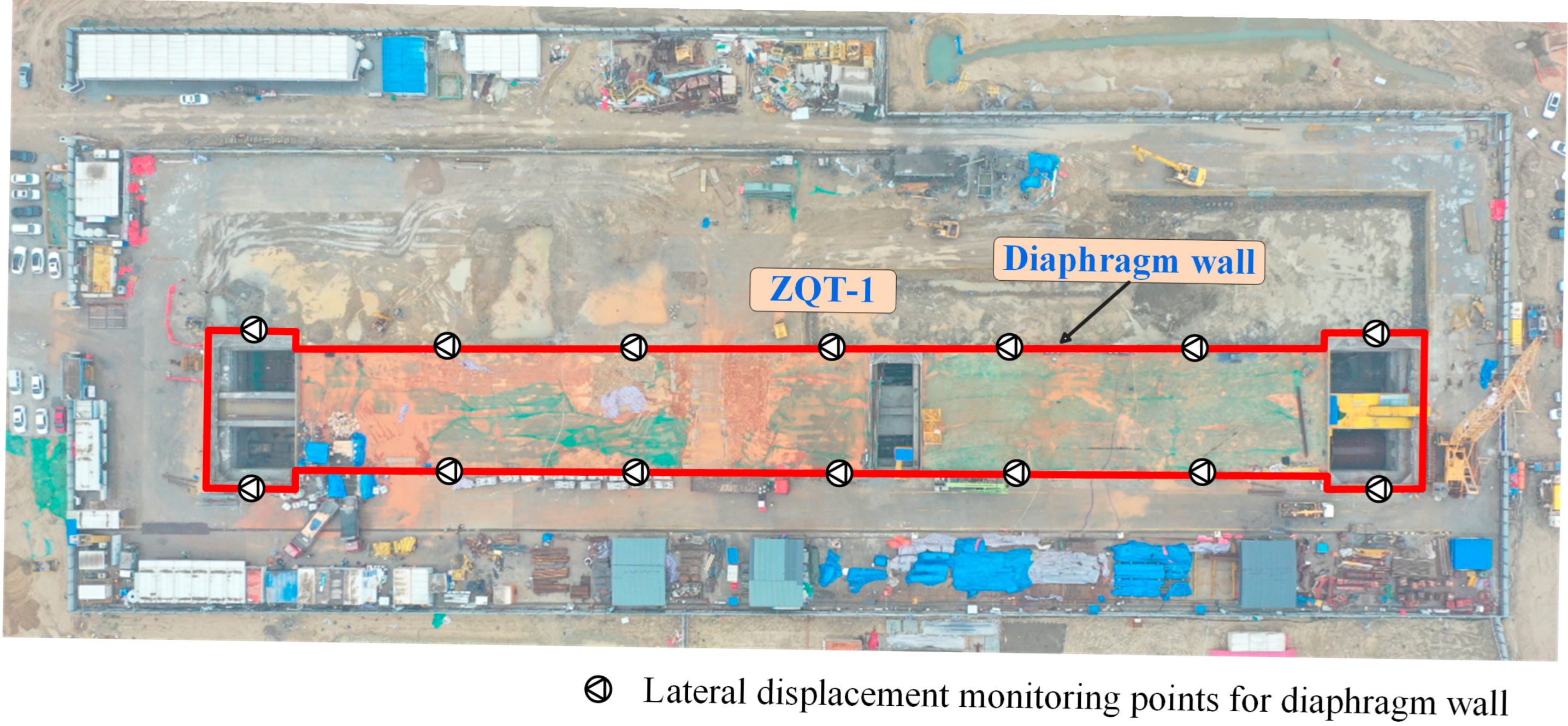
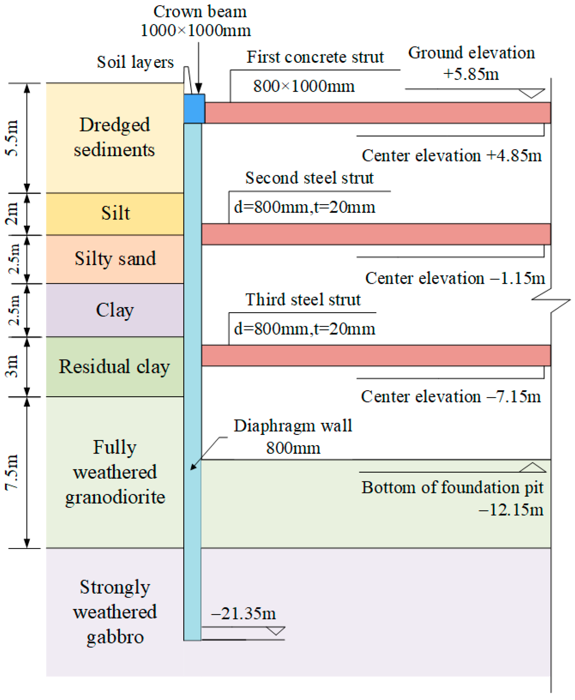
2.2.1. Engineering Background

The Airport Economic Zone Station of Xiamen Metro Line 3 is situated within the 15 km² dredger fill area of Dadeng Island. A deep layer of dredged sediments and an overlying silty sand stratum are present above the base slab of the foundation pit, making the site susceptible to infiltration-related deformation phenomena such as soil flow and piping during excavation. Geological investigation through borehole exploration revealed that the upper strata consist of recently deposited dredged sediments, silt, and silty sand; the middle strata are primarily composed of clay and residual clay; and the lower strata comprise fully weathered granodiorite or strongly weathered gabbro.

Throughout the excavation process, variations in lateral displacement were continuously recorded. An aerial view of the foundation pit and the layout of the monitoring points is shown in Figure 2. A total of 14 measurement points were installed for this project, with particular attention given to the lateral displacement of the retaining structure at monitoring point ZQT-1. A typical structural support schematic is provided in Figure 3.

The foundation pit is approximately rectangular in shape, with an excavation depth of about 18 m. The primary retaining system consists of an 800 mm thick underground diaphragm wall supported by internal struts. The first-level struts are reinforced concrete members spaced at 9 m intervals, while the remaining two levels are steel struts with 3 m spacing. According to the engineering report, the two liquefiable soil layers—dredged sediments and silty sand—within the excavation zone have a significant impact on deformation during excavation. This study focuses on the inversion of constitutive parameters for these two critical soil layers.

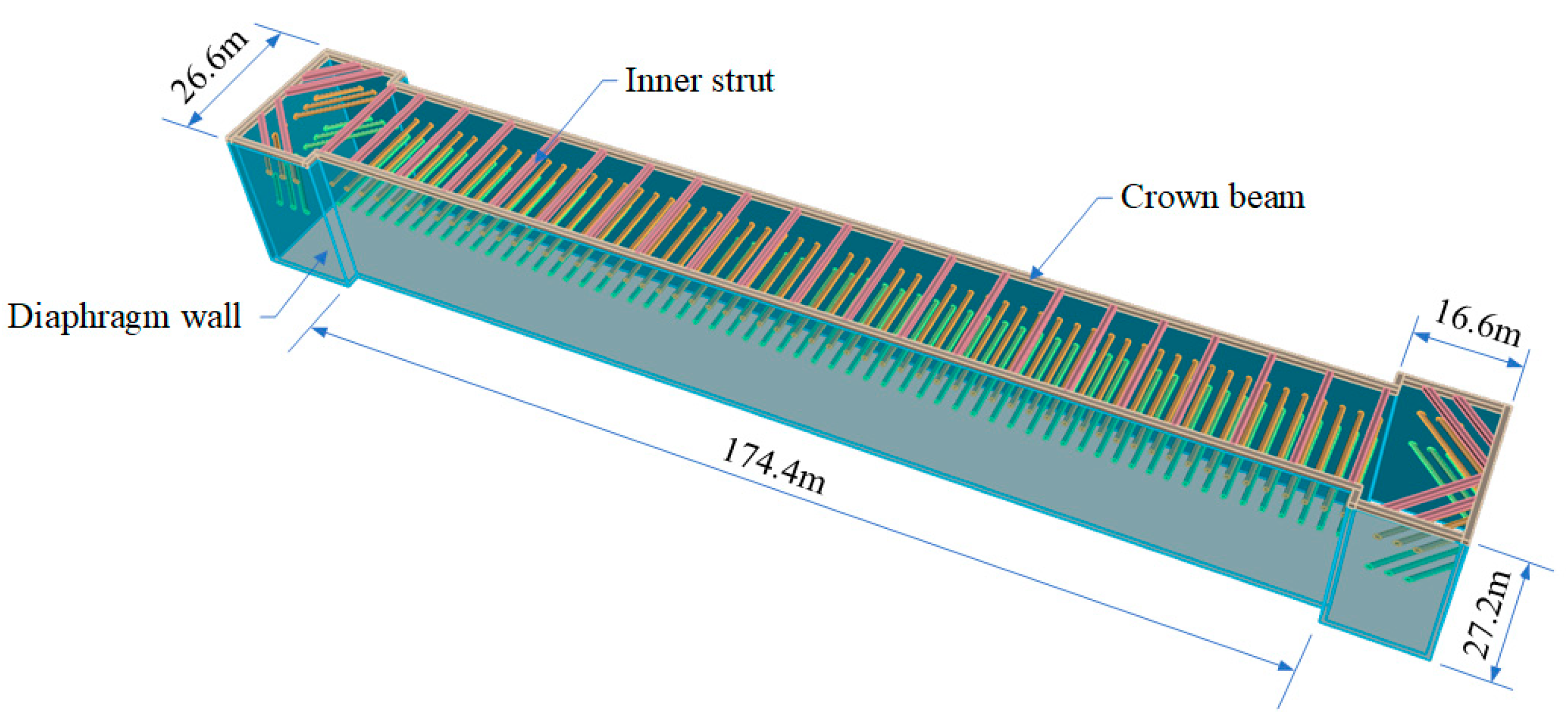
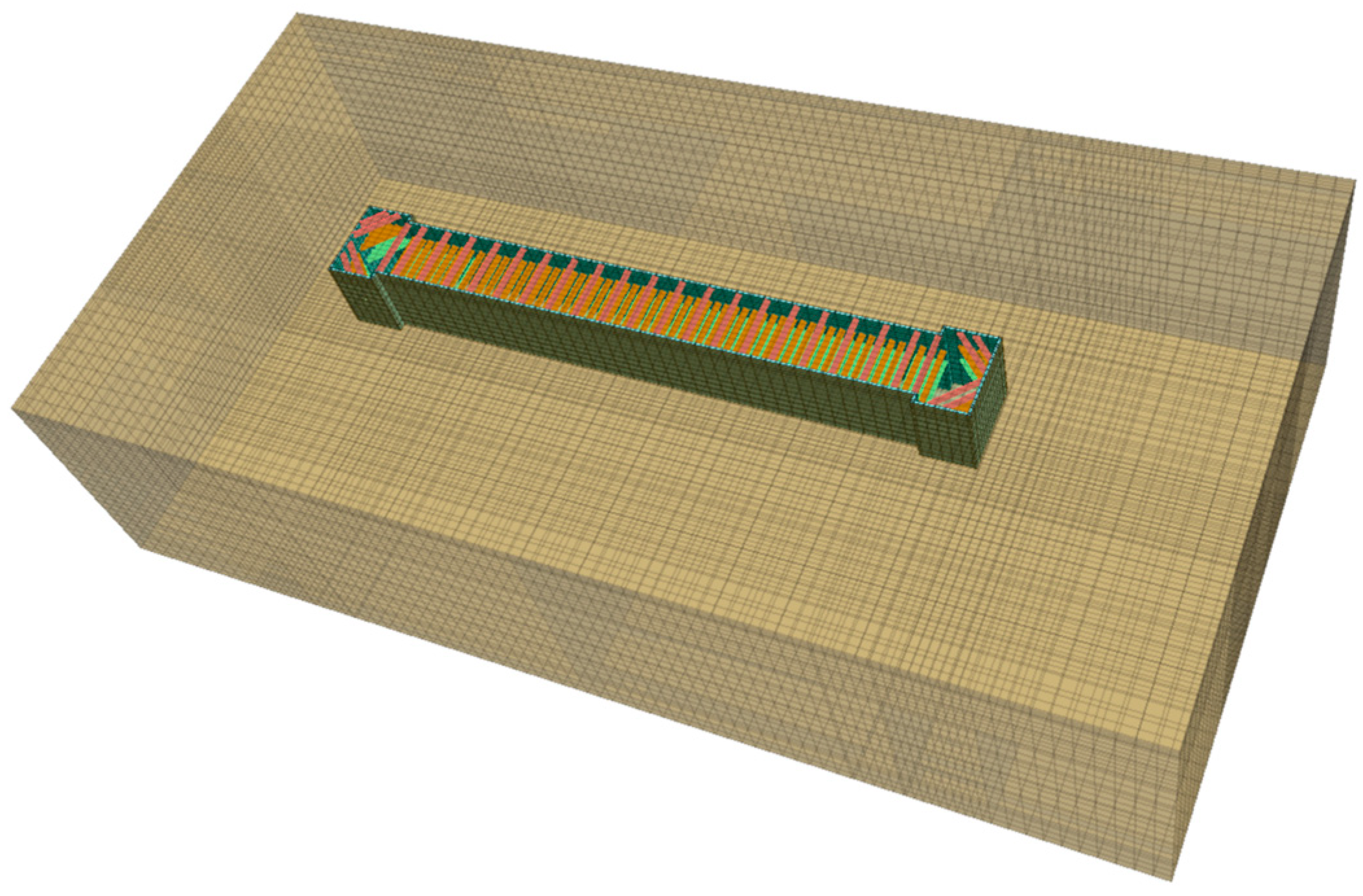
2.2.2. FLAC^3D Numerical Simulation

A three-dimensional finite element model of the foundation pit was developed using Rhino 7.0, as shown in Figure 4. According to past engineering practice and numerical simulation experience, the potential zone affected by foundation pit excavation is generally estimated to extend 2 to 3 times the depth of the excavation [26]. Therefore, the numerical calculation model in this paper takes the western boundary of the pit (the long side of the pit) as the X-axis, the northern boundary (the short side of the pit) as the Y-axis, and extends the distance of 4 times the depth of pit excavation from the boundary of pit excavation outward as the model side. The model dimensions are 386 m (length) × 206.6 m (width) × 90 m (height), as determined through finite element analysis. The detailed configuration of the three-dimensional numerical model and mesh layout is presented in Figure 5.

For the purposes of modeling and computing, the soil layers are represented as stratified and homogeneous in accordance with actual conditions. Prior to excavation, dewatering was conducted to lower the groundwater table below the base of the foundation pit. Given the short construction duration, the soil remained relatively dry throughout the excavation process; hence, groundwater seepage effects were not considered in the numerical analysis. A polyhedral volume mesh is used to simulate the retaining struts and the soil layer, with mesh refinement in areas close to the diaphragm wall. The boundaries of the model in the horizontal directions (i.e., x and y directions) are fixed, while the boundaries in the vertical direction are free. The bottom surface of the model is constrained in both normal and tangential displacements, whereas the top surface is treated as a free boundary.

The excavation of the foundation pit is carried out in five sequential construction stages due to site constraints. The detailed modeling of each construction phase is summarized in

Table 1. Simulation of construction stages.

Stage	Construction	Excavation Depth/m
CS 1	Excavate at 4.05~5.85 m, install the first level inner strut	1.5
CS 2	Excavate at −1.65~4.05 m, install the second level inner strut	7.5
CS 3	Excavate at −7.65~−1.65 m, install the third level inner strut	13.5
CS 4	Excavate at −9.65~−7.65 m	15
CS 5	Excavate at −12.15~−9.65 m	18

. Given the shallow excavation depth during the initial stages, the lateral deformation of the retaining wall is minimal and can be considered negligible. Therefore, construction stages 3 (CS3), 4 (CS4), and 5 (CS5) are selected for the parameter inversion analysis.

The HS model serves as the constitutive model for calculations, necessitating the input of 11 parameters in FLAC^3D 6.0 software for numerical analysis [27]. The four parameters, $E_{50}^{ref}$, ${\phi }^{\prime }$, $c^{\prime },$ and $E_{ur}^{ref},$ significantly influence the numerical simulation results, and based on engineering experience, there is a certain proportionality between the two parameters, $E_{ur}^{ref}$ and $E_{50}^{ref}$ [28]. Therefore, the parameters, including $E_{50}^{ref}$, ${\phi }^{\prime }$, $c^{\prime },$and the ratio between the $E_{ur}^{ref}$ and $E_{50}^{ref}$ of the two liquefied soil layers are selected as the parameters to be inverted.

The retaining structure is modeled using linear–elastic slab elements, while the internal support struts are represented by linear–elastic beam elements [29]. The detailed structural properties are summarized in

Table 2. Parameters of foundation pit retaining structure.

Materials	Density/(kg/m3)	Elasticity Modulus/(GPa)	Poisson’s Ratio	Size/(mm)
diaphragm wall	25	30	0.2	$800 \times 800$
concrete inner struts	25	30	0.2	$800 \times 1000$
steel inner struts	78	174	0.3	d = 800, t = 20

. The soil parameters employed in this study are primarily derived from previous geotechnical investigation reports and relevant site data. Certain parameters were appropriately modified based on local empirical formulas or default coefficients provided by the simulation software. Except for the parameters subject to inversion, the specific HS model parameters are listed in

Table 3. Values of model soil parameter.

Soil Layer	$\mathit{\gamma }/$(kg/m3)	${\mathit{c}}^{\mathit{\prime }}$/(kPa)	${\mathit{\phi }}^{\mathit{\prime }}/$(°)	${\mathit{E}}_{50}^{\mathit{r}\mathit{e}\mathit{f}}$/(MPa)	${\mathit{E}}_{\mathit{o}\mathit{e}\mathit{d}}^{\mathit{r}\mathit{e}\mathit{f}}$/(MPa)	${\mathit{E}}_{\mathit{u}\mathit{r}}^{\mathit{r}\mathit{e}\mathit{f}}$/(MPa)	${\mathit{K}}_0$	$\mathit{T}/\left(\mathbf{m}\right)$
Dredged sediments	18.1	-	-	-	$E_{50}^{ref}$	${k_{1}E}_{50}^{ref}$	0.6	5.5
Silt	17.4	5	0	5	5	20	0.7	2
Silty sand	17.4	-	-	-	$E_{50}^{ref}$	${k_{2}E}_{50}^{ref}$	0.7	2.5
Clay	19.8	17	15	15	15	60	0.77	2.5
Residual clay	18.5	23	14.9	20	20	80	0.75	3
Fully weathered granodiorite	21.0	35	26	40	40	150	0.7	7.5
Strongly weathered gabbro	24.0	45	30	60	60	200	0.58	-

T is the thickness of each soil layer, $\gamma$ is the soil density, $c^{\prime }$ is the effective cohesion, ${\phi }^{\prime }$ is the effective internal friction angle, $E_{50}^{ref}$, $E_{oed}^{ref}$, and $E_{ur}^{ref}$ are the elastic reference modulus, and $k_1$, $k_2$ are the ratio between the $E_{ur}^{ref}$ and $E_{50}^{ref}$.

.

In this case, the reference stress $p^{ref}$ is taken as 100 kPa; the unloading–reloading Poisson’s ratio is taken as 0.2 by using the recommended value in the FLAC^3D manual [30]; the exponent for elastic moduli $m$ is taken as 0.5; and the dilation angle $\psi$ is taken as 0 [31].

2.3. Orthogonal Experiment

2.3.1. Determination of Parameter Inversion Intervals

The soil parameters derived from geological survey reports lack sufficient accuracy, and direct numerical simulations utilizing these parameters may not yield the expected outcomes [32]. For this reason, parameter inversion techniques are employed to obtain more accurate soil properties. Even under identical control conditions, values obtained from in situ or laboratory tests can vary significantly, sometimes by several-fold. Therefore, when establishing the inversion range for parameter estimation, the upper and lower bounds should be appropriately expanded based on the values reported in geotechnical investigations or laboratory tests [33]. Based on the research of other scholars [34], the upper and lower bounds for the parameter inversion of the HS model for the soil layers in the dredger fill region of Xiamen were established at 1.5 and 0.5 times the parameters derived from the geological survey reports, respectively, as illustrated in

Table 4. Model training parameter levels.

Value	Dredged Sediments				Silty Sand
	${{\mathit{c}}_1}^{\mathit{\prime }}$/ (kPa)	${{\mathit{\phi }}_1}^{\mathit{\prime }}/$ (°)	${{\mathit{E}}_{50}^{\mathit{r}\mathit{e}\mathit{f}}}_1$/ (MPa)	${\mathit{k}}_1$	${{\mathit{c}}_2}^{\mathit{\prime }}$/ (kPa)	${{\mathit{\phi }}_2}^{\mathit{\prime }}/$ (°)	${{\mathit{E}}_{50}^{\mathit{r}\mathit{e}\mathit{f}}}_2$/ (MPa)	${\mathit{k}}_2$
Level 1	4	10	4	3	6	10	5	3
Level 2	5	12	5	3.5	7	12	6	3.5
Level 3	6	14	6	4	8	14	7	4
Level 4	7	16	7	4.5	9	16	8	4.5
Level 5	8	18	8	5	10	18	9	5
Level 6	9	20	9	5.5	11	20	10	5.5
Level 7	10	22	10	6	12	22	11	6
Level 8	11	24	11	6.5	13	24	12	6.5

.

An orthogonal experimental design was employed to generate 64 sets of HS model parameter combinations, incorporating 8 factors at 8 levels. Each parameter set was input into the numerical model of the foundation pit for simulation. The lateral displacement values of the retaining structure at monitoring point ZQT-1 across various depths and parameter combinations have been acquired. The parameters of the soil layer and the lateral displacement values of the retaining structure in each group are utilized as training samples, resulting in the construction of a training set of 64 groups.

2.3.2. Training Samples

Each sample ID corresponds to a specific parameter combination generated through the orthogonal experimental design, with detailed combinations listed in

Table A1. Orthogonal experiments design based on $\mathrm{L}64\left(8^9\right)$ orthogonal table.

Sample ID	${{\mathit{c}}_1}^{\mathit{\prime }}$/ (kPa)	${{\mathit{\phi }}_1}^{\mathit{\prime }}/$ (°)	${{\mathit{E}}_{50}^{\mathit{r}\mathit{e}\mathit{f}}}_1$/ (MPa)	${\mathit{k}}_1$	${{\mathit{c}}_2}^{\mathit{\prime }}$/ (kPa)	${{\mathit{\phi }}_2}^{\mathit{\prime }}/$ (°)	${{\mathit{E}}_{50}^{\mathit{r}\mathit{e}\mathit{f}}}_2$/ (MPa)	${\mathit{k}}_2$
1	4	10	4	3	6	10	5	3
2	4	12	6	4.5	10	20	11	6.5
3	4	14	8	6	11	24	6	4.5
4	4	16	10	5.5	7	14	12	5
5	4	18	9	3.5	13	16	7	6
6	4	20	11	4	9	22	9	3.5
7	4	22	5	6.5	8	18	8	5.5
8	4	24	7	5	12	12	10	4
9	5	10	7	4	11	18	12	6
10	5	12	5	3.5	7	12	6	3.5
11	5	14	11	5	6	16	11	5.5
12	5	16	9	6.5	10	22	5	4
13	5	18	10	4.5	8	24	10	3
14	5	20	8	3	12	14	8	6.5
15	5	22	6	5.5	13	10	9	4.5
16	5	24	4	6	9	20	7	5
17	6	10	10	5	13	20	8	3.5
18	6	12	8	6.5	9	10	10	6
19	6	14	6	4	8	14	7	4
20	6	16	4	3.5	12	24	9	5.5
21	6	18	7	5.5	6	22	6	6.5
22	6	20	5	6	10	16	12	3
23	6	22	11	4.5	11	12	5	5
24	6	24	9	3	7	18	11	4.5
25	7	10	9	6	8	12	9	6.5
26	7	12	11	5.5	12	18	7	3
27	7	14	5	3	13	22	10	5
28	7	16	7	4.5	9	16	8	4.5
29	7	18	4	6.5	11	14	11	3.5
30	7	20	6	5	7	24	5	6
31	7	22	8	3.5	6	20	12	4
32	7	24	10	4	10	10	6	5.5
33	8	10	5	5.5	9	24	11	4
34	8	12	7	6	13	14	5	5.5
35	8	14	9	4.5	12	10	12	3.5
36	8	16	11	3	8	20	6	6
37	8	18	8	5	10	18	9	5
38	8	20	10	6.5	6	12	7	4.5
39	8	22	4	4	7	16	10	6.5
40	8	24	6	3.5	11	22	8	3
41	9	10	6	6.5	12	16	6	5
42	9	12	4	5	8	22	12	4.5
43	9	14	10	3.5	9	18	5	6.5
44	9	16	8	4	13	12	11	3
45	9	18	11	6	7	10	8	4
46	9	20	9	5.5	11	20	10	5.5
47	9	22	7	3	10	24	7	3.5
48	9	24	5	4.5	6	14	9	6
49	10	10	11	3.5	10	14	10	4.5
50	10	12	9	4	6	24	8	5
51	10	14	7	6.5	7	20	9	3
52	10	16	5	5	11	10	7	6.5
53	10	18	6	3	9	12	12	5.5
54	10	20	4	4.5	13	18	6	4
55	10	22	10	6	12	22	11	6
56	10	24	8	5.5	8	16	5	3.5
57	11	10	8	4.5	7	22	7	5.5
58	11	12	10	3	11	16	9	4
59	11	14	4	5.5	10	12	8	6
60	11	16	6	6	6	18	10	3.5
61	11	18	5	4	12	20	5	4.5
62	11	20	7	3.5	8	10	11	5
63	11	22	9	5	9	14	6	3
64	11	24	11	6.5	13	24	12	6.5

. The predicted lateral displacements at monitoring point ZQT-1 are obtained by inputting each set of HS model soil parameters into the numerical model. A total of 64 parameter–displacement pairs were compiled as training samples, incorporating soil parameters and the corresponding lateral displacements at various depths. A subset of the training samples generated from the orthogonal experiment is presented in

Table 5. Partial orthogonal design training samples.

Construction Stage	Sample ID	Lateral Displacement of Diaphragm Wall at Different Depth/(mm)
		−4 m	−8 m	−12 m	−14 m	−16 m	−18 m	−22 m	−26 m
CS 3	1	3.79	5.33	7.04	8.69	9.01	8.37	6.25	4.31
	5	3.57	4.97	6.98	8.78	9.20	8.66	6.32	4.32
	9	3.44	4.64	6.87	8.81	9.27	8.75	6.49	4.46
	13	3.57	5.24	6.98	8.41	8.51	7.87	5.96	4.17
	17	3.55	4.98	6.62	8.08	8.25	7.65	5.88	4.05
	21	3.57	4.96	6.95	8.60	8.87	8.24	6.18	4.26
	25	3.40	4.70	7.20	9.06	9.45	8.87	6.53	4.43
	29	3.55	5.21	7.21	8.98	9.36	8.77	6.40	4.38
	33	3.49	5.07	6.98	8.73	9.12	8.58	6.30	4.33
	37	3.58	5.08	7.05	8.77	9.08	8.46	6.26	4.28
	41	3.60	5.07	6.93	8.53	8.76	8.13	6.09	4.16
	45	3.49	4.97	6.97	8.59	8.85	8.28	6.31	4.30
	49	3.54	4.93	6.87	8.55	8.85	8.33	6.31	4.36
	53	3.44	4.64	6.92	8.94	9.45	8.85	6.49	4.47
	56	3.66	5.31	7.03	8.40	8.45	7.74	5.84	4.04
	61	3.57	5.18	7.15	8.88	9.22	8.59	6.27	4.29
CS 4	2	4.76	5.97	9.87	11.69	13.83	13.46	10.07	6.78
	6	4.91	6.39	9.73	11.38	13.30	12.81	9.61	6.54
	10	4.99	6.61	9.81	11.96	14.08	13.70	10.25	6.94
	14	4.88	6.15	9.44	11.90	14.16	13.86	10.34	6.94
	18	4.94	6.24	9.48	11.97	14.18	13.81	10.11	6.77
	22	4.89	6.56	9.83	11.88	14.05	13.75	10.11	6.76
	26	4.91	6.39	9.61	11.96	14.19	13.89	10.19	6.72
	30	4.93	6.36	9.65	11.80	13.97	13.65	10.12	6.78
	34	4.99	6.18	9.57	11.39	13.39	13.00	9.74	6.58
	38	4.87	6.25	9.53	11.69	13.79	13.36	9.96	6.68
	42	4.85	6.20	9.54	11.79	14.04	13.72	10.01	6.81
	46	5.04	6.40	9.71	11.88	13.97	13.60	10.00	6.68
	50	4.90	6.30	9.62	11.71	13.87	13.49	10.00	6.70
	54	4.97	6.45	9.77	11.76	13.93	13.58	10.12	6.79
	57	4.98	6.31	9.64	11.65	13.73	13.33	9.95	6.64
	62	4.85	6.14	9.41	11.98	14.25	13.94	10.42	6.99
CS 5	3	8.12	8.79	13.33	15.56	21.71	23.07	16.57	10.99
	5	8.41	8.83	13.65	15.69	21.65	23.06	16.87	11.05
	8	8.60	8.84	13.81	15.85	21.82	23.27	17.03	11.22
	11	8.51	8.85	14.01	16.36	22.26	23.90	17.06	11.39
	16	8.66	8.88	13.83	15.84	21.78	23.18	16.98	11.12
	20	8.31	8.81	13.53	15.61	21.62	23.09	17.00	11.23
	26	8.42	8.80	13.79	16.18	22.35	23.60	16.89	10.91
	33	8.57	8.77	13.69	15.62	21.55	23.01	16.81	11.03
	36	8.48	8.84	13.72	15.70	21.61	22.97	16.80	10.95
	38	8.25	8.74	13.65	16.09	22.33	23.58	16.69	10.89
	42	8.43	8.76	13.64	15.69	21.66	23.05	16.94	11.11
	46	8.56	8.95	13.90	16.08	22.19	23.56	16.90	11.21
	50	8.47	8.80	13.68	15.72	21.73	23.15	16.83	11.04
	53	8.13	8.70	13.56	15.89	22.10	23.59	17.21	11.28
	59	8.37	8.74	13.69	15.89	21.96	23.38	17.01	11.12
	64	8.25	8.59	13.95	16.49	22.82	24.15	16.92	11.00

.

3. Results

3.1. Inversion Results of Soil Parameters

The Gray Wolf Optimization (GWO) algorithm is employed to optimize the parameters of the MLSSVR model, which is then applied to the inversion of soil parameters. The GWO-MLSSVR model is trained, using the sample data presented in Table 5, to construct a predictive regression model. For comparison purposes, an unoptimized MLSSVR model is also trained using the same dataset. The lateral displacement data of the retaining structure at varying depths, obtained from PVC inclinometer measurements, were input into the trained GWO-MLSSVR model to perform the inversion of the HS model parameters for the dredged sediment and silty sand layers. The results of the inversion are presented in

Table 6. Inversion results of soil parameters.

Construction Stage	Inversion Method	Dredged Sediments				Silty Sand
		${{\mathit{c}}_1}^{\mathit{\prime }}$/ (kPa)	${{\mathit{\phi }}_1}^{\mathit{\prime }}/$ (°)	${{\mathit{E}}_{50}^{\mathit{r}\mathit{e}\mathit{f}}}_1$/ (MPa)	${\mathit{k}}_1$	${{\mathit{c}}_2}^{\mathit{\prime }}$/ (kPa)	${{\mathit{\phi }}_2}^{\mathit{\prime }}/$ (°)	${{\mathit{E}}_{50}^{\mathit{r}\mathit{e}\mathit{f}}}_2$/ (MPa)	${\mathit{k}}_2$
CS 3	GWO-MLSSVR	8.15	20.22	7.26	4.83	10.21	18.69	8.33	4.66
	MLSSVR	6.92	17.25	6.52	5.03	9.18	15.09	7.85	5.15
CS 4	GWO-MLSSVR	8.36	23.47	7.03	5.01	13.19	17.34	8.85	4.78
	MLSSVR	6.01	19.04	5.23	4.82	11.23	14.68	8.24	5.31
CS 5	GWO-MLSSVR	8.55	22.64	6.52	4.52	12.01	17.14	8.74	4.86
	MLSSVR	6.13	20.30	5.14	4.44	10.12	15.55	8.28	5.10

.

3.2. Assessment of Inversion Performance

The inversion findings were re-entered into the numerical model of the foundation pit for analysis, yielding the lateral displacement values of the retaining structure at the measurement points, which were subsequently compared with the actual monitoring data. Figure 6 presents a comparison between the predicted displacements obtained from the GWO-MLSSVR and MLSSVR inversion models and the measured data across different construction stages. RMSE represents the root mean square error between the predicted and measured displacements, while MAE denotes the mean absolute error. As shown, the displacement curves derived from both GWO-MLSSVR and MLSSVR closely match the actual monitoring data. With the progression of construction stages, the lateral displacement of the retaining structure increases continuously, and both RMSE and MAE of the predicted displacements also show an increasing trend. Notably, the GWO-MLSSVR model consistently yields lower RMSE and MAE values compared to the standard MLSSVR model, indicating improved prediction accuracy.

Figure 7 illustrates the relative errors between the measured and predicted displacements of the retaining structure at various depths across different construction stages. The Mean Relative Error (MRE) represents the average relative difference between the predicted and measured displacements. In Construction Stage 3, the GWO-MLSSVR model achieved an MRE of 5.99%, with a maximum relative error of 16.53%, whereas the MLSSVR model resulted in a higher MRE of 12.98% and a maximum relative error of 27.44%. In Stage 4, the GWO-MLSSVR model further improved, yielding an MRE of 4.16% and a maximum relative error of −8.14%, compared to the MLSSVR model’s MRE of 12.22% and a maximum relative error of −22.17%. In Stage 5, the GWO-MLSSVR model reached its best performance, with an MRE of 2.69% and a maximum relative error of 4.11%, while the MLSSVR model produced an MRE of 10.80% and a maximum relative error of 21.18%. Moreover, as the excavation progresses, the inverted lateral displacement of the retaining structure increases progressively, while the relative error decreases and gradually stabilizes.

Figure 8 presents the ${\mathrm{R}}^2$ values of the inversion results obtained from the GWO-MLSSVR and MLSSVR models. As the ${\mathrm{R}}^2$ values close to 1 indicate a high degree of agreement between the predicted and actual values, they reflect better model-fitting performance. Across all construction stages, the ${\mathrm{R}}^2$ values of the GWO-MLSSVR model are consistently higher than those of the MLSSVR model. When considered alongside other evaluation metrics, such as MAE, RMSE, and MRE, these results suggest that the inversion performance of GWO-MLSSVR is superior to that of the standard MLSSVR model. The GWO-MLSSVR model is an innovative and practical method for inverting the constitutive parameters of foundation soils and it exhibits excellent inversion accuracy.

The prediction errors may be primarily attributed to the simplifications made during the numerical simulation process when representing real conditions. The training samples used for parameter inversion were generated through numerical simulations, which involved certain assumptions to reduce computational complexity. For example, the complex stratigraphy of the soil layers was simplified into a homogeneous model, and localized soil features were neglected. These simplifications can influence the simulation accuracy of soil deformation and the internal forces of the retaining structure, potentially leading to discrepancies between the simulation results and actual field measurements. Moreover, validation of the inversion results also relies on numerical simulations to predict the horizontal displacement of the retaining structure, which may introduce additional sources of error. Factors such as the number of training samples and the number of input nodes in the model can also impact prediction accuracy—these aspects will be further discussed in the following sections. Nevertheless, the inversion errors of the GWO-MLSSVR model can be maintained within a very small range, fully meeting the accuracy requirements of practical engineering applications. Therefore, the GWO-MLSSVR-based inversion method can be regarded as an innovative and practical approach for identifying the constitutive parameters of foundation soils, offering high precision and reliability in parameter estimation.

4. Discussion

4.1. Effect of Construction Stage

The excavation of pits is a dynamic process; therefore, relying just on the inversion parameters of the corresponding construction stage for comparison is inadequate. The inverted soil parameters are inputted into the finite element model to calculate the displacement values for the next stage. The soil parameters derived from the inversion in construction stages 3 (CS 3) and 4 (CS 4) are utilized to predict the lateral displacement of the retaining structure at construction stages 5 (CS 5). The result is then compared with the lateral displacement of the retaining structure obtained from the inversion of CS 5 and the actual monitored displacement, as illustrated in Figure 9.

As can be seen in Figure 9, the predicted displacement curves using the parameters obtained from CS 3 and CS 4 failed to outperform the predicted displacement curves of CS 5. The predicted displacement curves of CS 5 are closer to the monitored displacement curves. In addition, the RMSE and MAE of the predicted values of the inversion parameters of CS 5 are smaller than the predicted values of the inversion parameters of CS 3 and CS 4, and its R² value is better than that of the inversion parameters of CS 3 and CS 4. The reasons for this situation are due to the facts that the displacement change in the subsequent condition of pit excavation is larger than that of the preceding condition and that it is more effective to directly use the condition with large displacement change in the inversion when performing the parameter inversion. The results indicate that using the inversion parameters of the subsequent construction stage to forecast the displacements of their corresponding construction stage is more effective than utilizing the prior construction stage. The data update facilitates a more precise process of inversion and forecasting.

4.2. Compared with Other Inversion Methods

Previous studies have applied artificial neural networks (ANNs) to establish the nonlinear relationship between rock mass mechanical parameters and observed displacements, thereby enabling parameter back-analysis [12]. ANNs are more suitable for processing large-scale, complex, or unstructured data. In contrast, MLSSVR is based on support vector regression combined with least squares optimization, aiming to identify a hyperplane that minimizes the squared prediction error. However, when applied to the inversion of soil parameters based on measured displacement data, ANNs may encounter issues such as convergence to local optima and instability during training. In this study, commonly adopted inversion methods, including Random Forest and PSO-BP (Particle Swarm Optimization–Backpropagation), are trained using the dataset provided in Table 5. A comparative analysis of their inversion performance under construction stage 5 is illustrated in Figure 10.

The relative errors of the retaining structure’s lateral displacements at various points were statistically analyzed, and the Confidence Intervals (CI) of the relative errors in predicted displacements were calculated to illustrate the differences in inversion performance among the models. The confidence intervals of the predicted displacements obtained from each model are presented in

Table 7. CI of relative errors in predicted displacements.

Inversion Method	MRE (%)	95% CI (%)	99% CI (%)
RF	9.50	[−5.80, 7.10]	[−8.40, 9.70]
PSO-BP	7.65	[−1.78, 8.60]	[−3.86, 10.68]
GWO-MLSSVR	2.69	[−0.88, 3.18]	[−1.49, 3.79]

.

The notation “95% CI” refers to the 95% confidence interval, while “99% CI” denotes the 99% confidence interval. Under an acceptable confidence level, the prediction error confidence intervals derived from the GWO-MLSSVR model consistently exhibit a shorter interval length compared to those of the other two models. Moreover, both the upper and lower bounds of the GWO-MLSSVR confidence intervals are significantly lower than those of the alternatives. The length of a confidence interval reflects the variability or uncertainty in prediction errors—a shorter interval indicates reduced error fluctuation, suggesting that the outputs of the GWO-MLSSVR model are more concentrated and stable. The upper and lower bounds of the confidence interval are closer to zero, indicating that the GWO-MLSSVR model yields smaller prediction errors and achieves higher predictive accuracy compared to the other two models.

A detailed comparison of the three models—Random Forest (RF), PSO-BP, and GWO-MLSSVR—indicates that the GWO-MLSSVR model achieves the best overall performance in the inversion of soil layer parameters. It outperforms the other two models across all evaluation metrics, including RMSE, MAE, MRE, and R², demonstrating the smallest prediction errors, superior fitting accuracy, and stronger generalization capability. These results suggest that GWO-MLSSVR provides more effective inversion results in this work and holds greater potential for practical application.

This can be attributed to the fact that in most inversion analyses, the available dataset is relatively limited in size. The GWO-MLSSVR model exhibits enhanced generalization ability, especially under small-sample conditions, where it delivers more stable and accurate predictions. In contrast, the PSO-BP neural network generally requires a large amount of training data to perform reliably, and its performance may degrade significantly when the data are insufficient. RF, which relies on the ensemble of multiple decision trees to achieve robustness, requires a certain degree of sample diversity to support its ensemble advantage; under small-sample conditions, the uncertainty in the constructed trees may lead to unstable or biased predictions.

4.3. Compared with Other Optimization Algorithms

To verify the effectiveness of using the GWO to optimize the parameters of the MLSSVR model, this study compares it with two commonly used optimization algorithms: Genetic Algorithm (GA) and Particle Swarm Optimization (PSO). Using the same training samples, the GA-MLSSVR and PSO-MLSSVR models are built for parameter inversion using the training samples of construction stage 5 as an example. Compare the performance of MLSSVR models constructed by different optimization algorithms in terms of prediction error and stability. A detailed comparison of the inversion results during construction stage 5 is illustrated in Figure 11.

As shown in Figure 11, the MLSSVR models optimized by the three algorithms all exhibit higher R² values compared to the non-optimized MLSSVR model. Moreover, the optimized models demonstrate significantly lower values of MRE, MAE, and RMSE in displacement prediction, indicating that all three optimization algorithms effectively enhance the performance of the MLSSVR model. Among them, the GWO-MLSSVR model achieves the lowest prediction errors, suggesting that it delivers the best optimization results. The GWO-MLSSVR also shows the smallest MRE in displacement prediction, which implies that the multi-leader cooperation mechanism of GWO effectively helps avoid local optima. In contrast, although the PSO- and GA-optimized models produce displacement predictions close to actual values at certain depths, they still yield larger overall errors. This can be attributed to PSO’s tendency for premature convergence when the inertia weight is improperly set and to GA’s unstable convergence path, which performs poorly when the number of training samples is limited. Additionally, GWO requires tuning only two parameters—the number of individuals and the maximum number of iterations—without involving complex weight or probability settings. This simplicity makes it significantly more efficient and user-friendly for parameter inversion compared to GA and PSO, with much lower tuning costs.

4.4. Effect of Node Number in the Input Layer

This paper uses lateral displacement of the retaining structure at different depths of the measurement point as the input layer based on the nonlinear mapping relationship between the soil parameters of the pit and the deformation of the retaining structure. In this example, the number of nodes of the input layer used is eight, which represents the lateral displacement of the retaining structure at eight different depths. To study the influence of the number of nodes of the input layer on the GWO-MLSSVR model, the number of nodes of the input layer is set to 5, 6, 7, 8, 9, and 10. The lateral displacement of the retaining structure at different excavation depths is taken as the input when the pit is excavated up to construction stage 5 and the inversion results of the soil parameters are output. The soil parameters were inputted into the numerical model of the foundation pit to obtain the predicted values of the lateral displacements of the retaining structure at the measurement points.

Table 8. Prediction error of measurement points with different input layer node numbers.

Number of Nodes in the Input Layer	Maximum Relative Error/%	Mean Relative Error/%	R2	Total CPU Time/s
5	24.03	13.32	0.73	193
6	19.67	8.20	0.88	330
7	9.34	5.61	0.94	524
8	4.12	2.69	0.99	667
9	4.01	2.62	0.99	1004
10	3.89	2.57	0.99	1760

lists the maximum relative error, mean relative error, R², and total CPU time of the prediction results with respect to the number of nodes in the input layer.

Table 8 indicates that both the maximum relative error and the mean relative error diminish as the number of nodes increases and the R² value rises with the addition of nodes; however, the marginal benefits are declining. When the number of nodes surpasses eight, the input layer’s node count exceeds that of the output layer; the highest relative error diminishes from 4.12% to 3.89% and the average relative error falls from 2.69% to 2.57%, but the enhancement of the R² value is minimal. The rate of error reduction diminishes, signifying that the training result approaches stabilization. However, further increasing the number of nodes in the input layer does not significantly reduce the error, while the CPU time necessary for training escalates. This is because the number of nodes in the input layer represents the dimensionality of the model’s input features. A greater number of nodes allows the model to access more information, potentially enhancing its learning ability. However, it may also introduce redundant information or noise. The number of input layer nodes directly affects the model’s capacity to learn from the input parameters and to represent features effectively. When the number of input nodes is set to five, the GWO-MLSSVR model may fail to capture sufficient input information, resulting in underfitting. In contrast, an excessive number of input nodes can lead the model to learn not only meaningful features but also irrelevant ones. This not only increases CPU time but may also cause overfitting, ultimately reducing the model’s generalization performance. Therefore, an appropriate number of input nodes should be selected to ensure the desired level of accuracy is achieved.

4.5. Effect of the Number of Training Samples

In this study, the training samples were generated through numerical simulations. Increasing the number of samples would significantly raise the computational workload. Therefore, based on the original 64 training sets, an additional 32 samples were generated by taking the average values between adjacent parameter sets, thereby expanding the dataset. To investigate the effect of training sample size on the inversion performance of the GWO-MLSSVR model, a series of datasets containing 16, 32, 48, 64, 80, and 96 samples were uniformly selected for parameter inversion. Under construction stage 5, the maximum relative error and mean relative error at the monitoring point corresponding to each sample size are presented in Figure 12.

When the number of training samples is 16, the maximum relative error is 24.15% and the mean relative error is 15.34%, indicating that the inversion results have large errors and poor accuracy. As the number of training samples increases, the prediction errors at the monitoring point are significantly reduced. When the training set size reaches 64, the maximum relative error is 4.11% and the mean relative error is 2.69%, showing a clear improvement in inversion performance. Although further increasing the number of training samples still slightly reduces the error, the marginal benefit becomes negligible. Moreover, a larger number of training samples considerably increases the workload of numerical simulations. Therefore, once the inversion accuracy meets engineering requirements, it is not necessary to further expand the training set. Herein, the use of 64 training samples provides a reasonable balance between computational effort and inversion accuracy, which meets practical engineering needs.

4.6. Research Limitation

The study proposes a method for precisely acquiring soil parameters, but some restrictions persist. This study conducts numerical simulations to generate training data for the machine learning model. The division of soil layers is simplified, which cannot completely simulate the actual conditions of the pit excavation and requiring additional refinement. During parameter inversion, it is essential to reasonably select the number of nodes in the input layer; otherwise, it might increase the computational burden and duration of the machine learning model. The appropriate number of training samples should be selected to balance the accuracy of the inversion and the computational workload of numerical simulation. Given that the inversion method was developed using a relatively limited training dataset, there is a potential risk of overfitting during inversion and prediction, which should be monitored and mitigated by tuning hyperparameters accordingly. Although the dataset employed originates from a dredger fill strata site, the proposed modeling approach is not dependent on the physical characteristics of a specific stratum, demonstrating a certain degree of generalizability. Nevertheless, further validation using field data from other regions is required before broader practical application can be ensured.

5. Conclusions

This study proposes an efficient and accurate parameter inversion method, demonstrated through a deep foundation pit project in Xiamen City involving dredger fill strata. A finite element model of the foundation pit was developed, and training samples for the inversion were generated using an orthogonal test design, comprising 64 sets of HS constitutive parameters for each of the three construction stages. The GWO-MLSSVR model was employed to invert the soil parameters of the two primary soil layers: dredged sediments and silty sand. The finite element analysis results based on the inverted parameters were compared with those obtained using MLSSVR and other inversion methods, leading to the following conclusions:

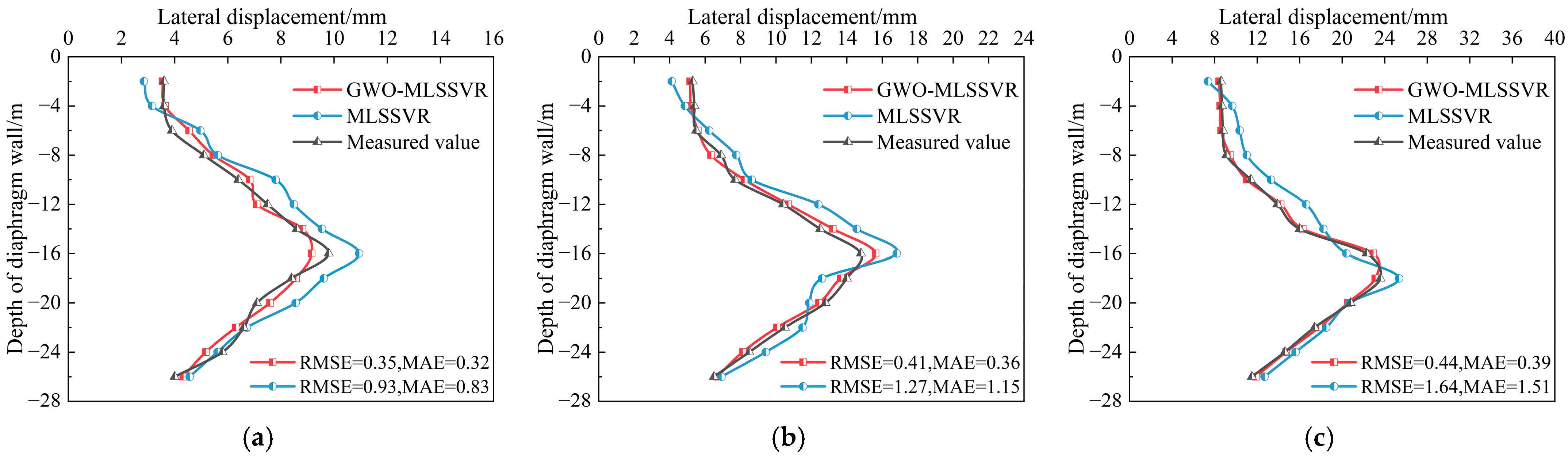
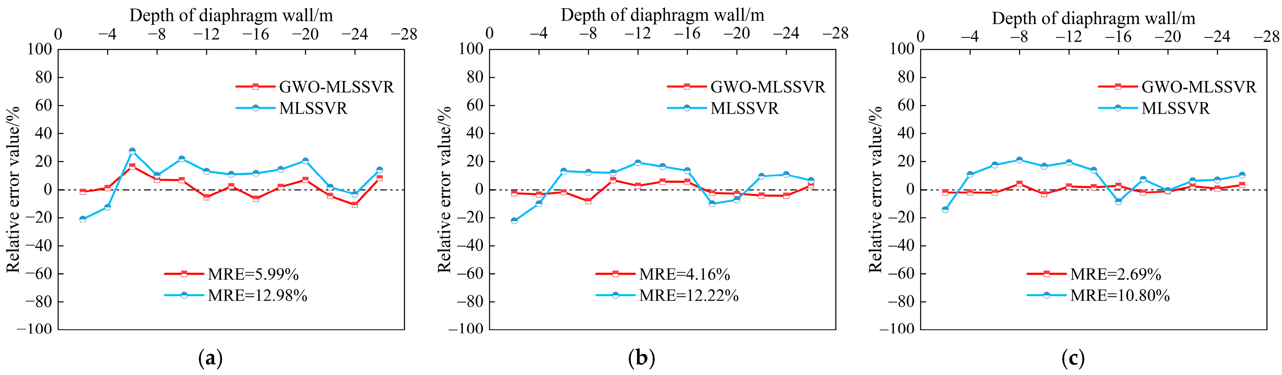
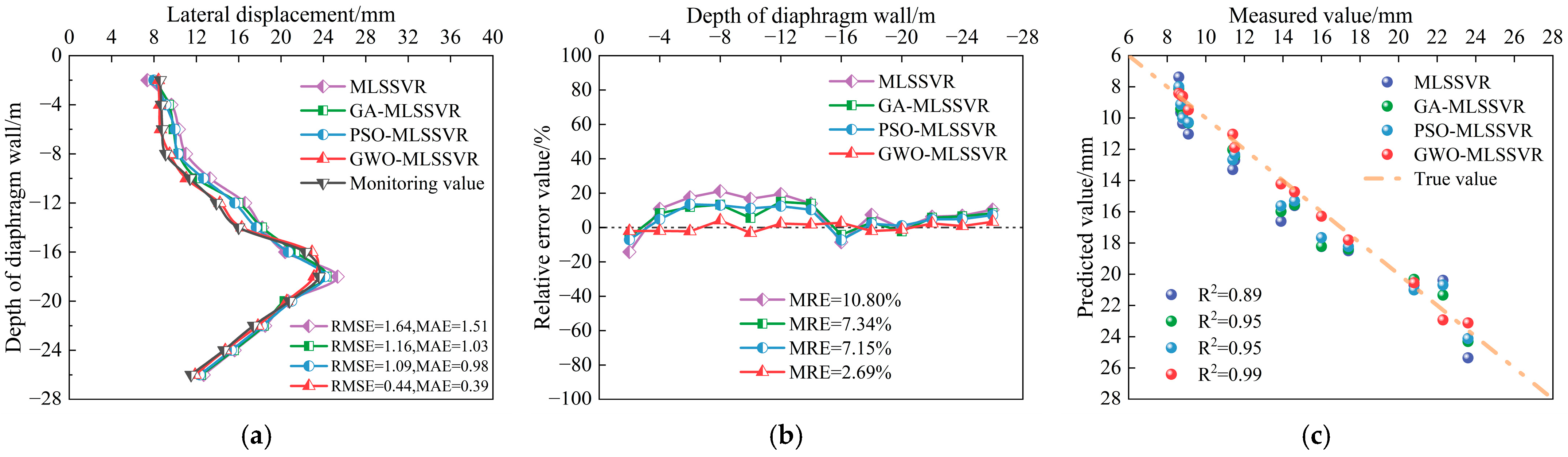
• The displacement curves of the retaining structure, obtained from the inversion of MLSSVR and GWO-MLSSVR, align with the variations in the actual displacement curves, indicating that the lateral displacement of the retaining structure can be accurately inverted to yield precise HS parameters. The lateral displacement values derived via GWO-MLSSVR closely align with the measured monitoring data, exhibiting reduced relative errors.
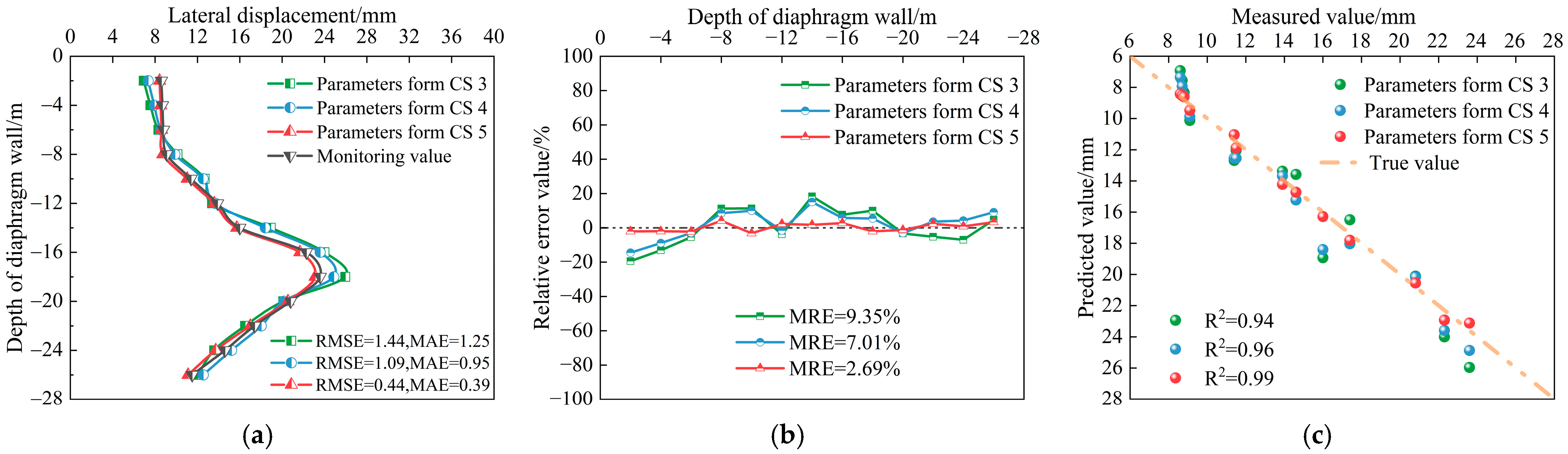
• With the progression of foundation pit excavation, the relative error in the inverted lateral displacements of the retaining structure tends to decrease. Hence, it is advisable to perform parameter inversion based on excavation stages with larger horizontal displacements, as this can lead to improved inversion accuracy.
• In the inversion method proposed in this study, increasing the number of input layer nodes can help reduce errors to a certain extent. However, when the error falls within the acceptable range for engineering applications, it is advisable to select an appropriate number of input nodes to avoid unnecessary computational costs and potential overfitting.
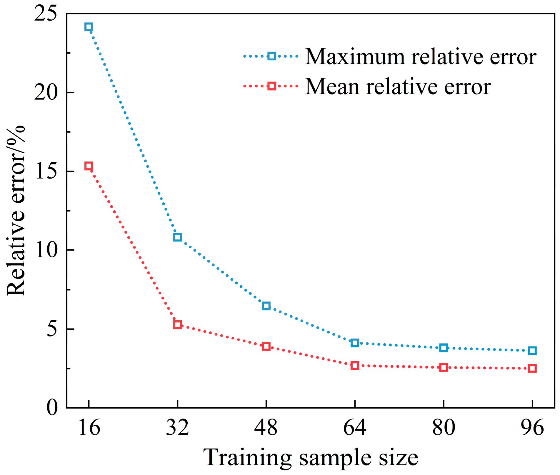
• The size of the training dataset has a certain impact on the inversion outcomes. In this study, 64 training samples were employed, which proved adequate to satisfy the accuracy requirements of parameter inversion.
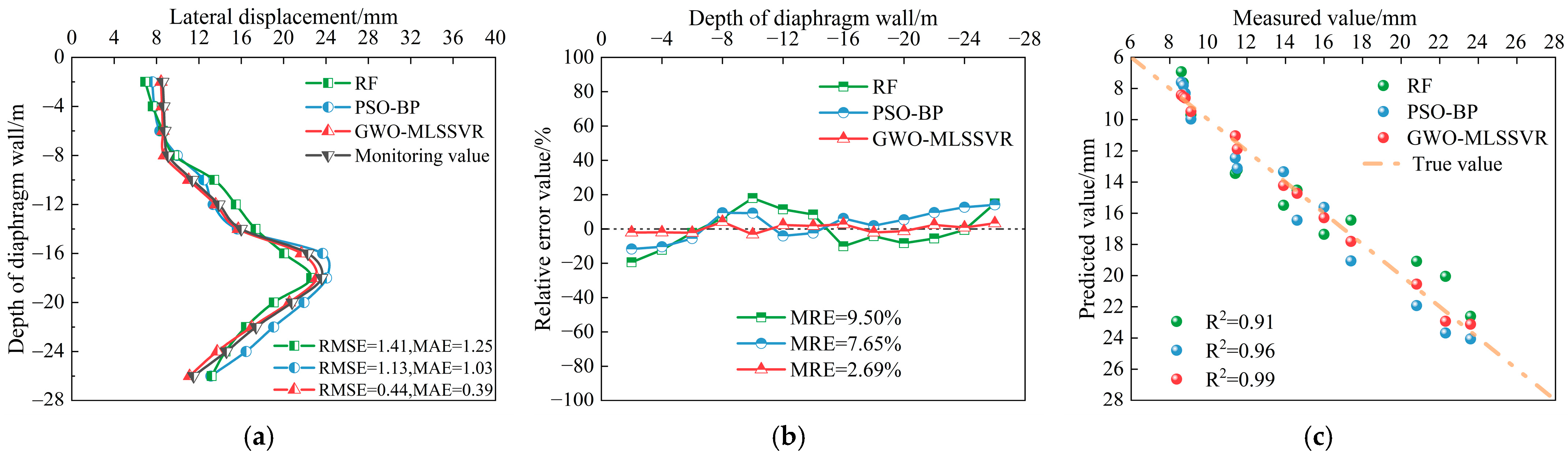
• Compared with other commonly adopted inversion methods, the GWO-MLSSVR method proposed in this study shows superior inversion performance. The lateral displacements of the retaining structure at various depths, calculated using the inverted parameters, differ from the measured values by less than 5%. This indicates that GWO-MLSSVR is an innovative and practical approach for inverting constitutive parameters of foundation soils, characterized by high accuracy and robustness.

References

1. Fu, Y.B.; He, S.Y.; Zhang, S.Z.; Yang, Y. Parameter Analysis on Hardening Soil Model of Soft Soil for Foundation Pits Based on Shear Rates in Shenzhen Bay, China. Adv. Mater. Sci. Eng. 2020, 2020, 7810918. [Google Scholar] [CrossRef]
2. Zhu, M.; Chen, X.S.; Zhang, G.T.; Pang, X.C.; Su, D.; Liu, J.Q. Parameter back-analysis of hardening soil model for granite residual soil and its engineering applications. Rock Soil Mech. 2022, 43, 1061–1072. [Google Scholar] [CrossRef]
3. Shi, X.M.; Sun, J.L.; Qi, Y.; Zhu, X.Y.; Zhang, X.M.; Liang, R.S.; Chen, H.J. Study on Stiffness Parameters of the Hardening Soil Model in Sandy Gravel Stratum. Appl. Sci. 2023, 13, 2710. [Google Scholar] [CrossRef]
4. Yan, X.; Tong, L.Y.; Li, H.J.; Liu, W.Y.; Xiao, Y.; Wang, W. Effects of the excavation of deep foundation pits on an adjacent double-curved arch bridge. Undergr. Space 2025, 21, 164–177. [Google Scholar] [CrossRef]
5. Cao, Y.M.; Li, Z.Y.; Chen, J.L.; Xia, C.Y. Stochastic inversion of soil dynamic parameters based on non-intrusive data. Soil Dyn. Earthq. Eng. 2024, 181, 108640. [Google Scholar] [CrossRef]
6. Pu, X.S.; Huang, J.; Peng, T.; Wang, W.Z.; Li, B.; Zhao, H.T. Application of Parameter Inversion of HSS Model Based on BP Neural Network Optimized by Genetic Algorithm in Foundation Pit Engineering. Buildings 2025, 15, 531. [Google Scholar] [CrossRef]
7. Cheng, Q.; Yang, Z.; Qin, S.; Zhang, L.; Miao, Q.; Zhang, Y. Application of soil parameters inversion based on psomlssvr in deep foundation pit engineering. J. Eng. Geol. 2022, 30, 520–532. [Google Scholar]
8. Zhang, J.J.; Li, H.B.; Zhang, G.Z.; Gu, Y.P.; Liu, Z.F. Rock physics inversion based on an optimized MCMC method. Appl. Geophys. 2021, 18, 288–298. [Google Scholar] [CrossRef]
9. Yaseen, Z.M.; Deo, R.C.; Hilal, A.; Abd, A.M.; Bueno, L.C.; Salcedo-Sanz, S.; Nehdi, M.L. Predicting compressive strength of lightweight foamed concrete using extreme learning machine model. Adv. Eng. Softw. 2018, 115, 112–125. [Google Scholar] [CrossRef]
10. Raja, M.N.A.; Abdoun, T.; El-Sekelly, W. Exploring the Potential of Machine Learning in Stochastic Reliability Modelling for Reinforced Soil Foundations. Buildings 2024, 14, 954. [Google Scholar] [CrossRef]
11. Tang, R.; Luo, W. Parameter inversion of soft soil subgrade based on support vector machine optimized by gravitational search algorithm. J. Rail Way Sci. Eng. 2022, 19, 1568–1576. [Google Scholar]
12. Yu, H.; Chen, X.B.; Yi, L.Q.; Qiu, J.; Gu, Z.H.; Zhao, H. Parameter inversion and application of soft soil modified Cambridge model. Rock Soil Mech. 2023, 44, 3318–3326. [Google Scholar] [CrossRef]
13. Sun, P.M.; Bao, T.F.; Gu, C.S.; Jiang, M.; Wang, T.; Shi, Z.W. Parameter sensitivity and inversion analysis of a concrete faced rock-fill dam based on HS-BPNN algorithm. Sci. China-Technol. Sci. 2016, 59, 1442–1451. [Google Scholar] [CrossRef]
14. Ruan, Y.; Yu, D.; Yang, J.; Wu, L.; Tan, G. Inversion of Mechanical Parameters of Reinforced Soft Soil around Tunnel Based on PSO-SVM. J. Highw. Transp. Res. Dev. 2020, 37, 87–96. [Google Scholar]
15. Cui, J.Q.; Wu, S.C.; Cheng, H.Y.; Kui, G.; Zhang, H.R.; Hu, M.L.; He, P.B. Composite interpretability optimization ensemble learning inversion surrounding rock mechanical parameters and support optimization in soft rock tunnels. Comput. Geotech. 2024, 165, 105877. [Google Scholar] [CrossRef]
16. Xiao, J.F.; Wang, Q.W.; Zhang, Q.H.; Hei, Y.P.; Zhang, Y.L. Multiple Parameters Determination Method of Hardening Soil Model Based on Particle Swarm Optimization. Adv. Civ. Eng. 2024, 2024, 5561981. [Google Scholar] [CrossRef]
17. Balogun, A.L.; Rezaie, F.; Pham, Q.B.; Gigovic, L.; Drobnjak, S.; Aina, Y.A.; Panahi, M.; Yekeen, S.T.; Lee, S. Spatial prediction of landslide susceptibility in western Serbia using hybrid support vector regression (SVR) with GWO, BAT and COA algorithms. Geosci. Front. 2021, 12, 101104. [Google Scholar] [CrossRef]
18. Tikhamarine, Y.; Souag-Gamane, D.; Ahmed, A.N.; Kisi, O.; El-Shafie, A. Improving artificial intelligence models accuracy for monthly streamflow forecasting using grey Wolf optimization (GWO) algorithm. J. Hydrol. 2020, 582, 124435. [Google Scholar] [CrossRef]
19. Guo, Z.; Liu, R.; Gong, C.; Zhao, L. Study on improvement of gray wolf algorithm. Appl. Res. Comput. 2017, 34, 3603. [Google Scholar]
20. Suykens, J.A.K.; Vandewalle, J. Least squares support vector machine classifiers. Neural Process. Lett. 1999, 9, 293–300. [Google Scholar] [CrossRef]
21. Zhou, J.; Qiu, Y.G.; Zhu, S.L.; Armaghani, D.J.; Li, C.Q.; Nguyen, H.; Yagiz, S. Optimization of support vector machine through the use of metaheuristic algorithms in forecasting TBM advance rate. Eng. Appl. Artif. Intell. 2021, 97, 104015. [Google Scholar] [CrossRef]
22. Chang, C.C.; Lin, C.J. LIBSVM: A Library for Support Vector Machines. ACM Trans. Intell. Syst. Technol. 2011, 2, 1–27. [Google Scholar] [CrossRef]
23. Wang, Y.K.; Tang, H.M.; Huang, J.S.; Wen, T.; Ma, J.W.; Zhang, J.R. A comparative study of different machine learning methods for reservoir landslide displacement prediction. Eng. Geol. 2022, 298, 106544. [Google Scholar] [CrossRef]
24. Zhang, L.M.; Wu, X.G.; Zhu, H.P.; AbouRizk, S.M. Performing Global Uncertainty and Sensitivity Analysis from Given Data in Tunnel Construction. J. Comput. Civ. Eng. 2017, 31, 04017065. [Google Scholar] [CrossRef]
25. Bao, T.F.; Li, J.M.; Lu, Y.F.; Gu, C.S. IDE-MLSSVR-Based Back Analysis Method for Multiple Mechanical Parameters of Concrete Dams. J. Struct. Eng. 2020, 146, 04020155. [Google Scholar] [CrossRef]
26. Ye, J.; He, X. Performance of batter pile walls in deep excavation: Laboratory test and numerical analysis. Mech. Adv. Mater. Struct. 2022, 29, 5301–5310. [Google Scholar] [CrossRef]
27. Li, Y.D.; Wang, C.X.; Sun, Y.; Wang, R.C.; Shao, G.J.; Yu, J. Analysis of Corner Effect of Diaphragm Wall of Special-Shaped Foundation Pit in Complex Stratum. Front. Earth Sci. 2022, 10, 794756. [Google Scholar] [CrossRef]
28. Shi, Y.; Ruan, J.; Wu, C. Xiamen area typical stratum of HS-small model for small strain parameters sensitivity analysis. Sci. Technol. Eng. 2017, 17, 105–110. [Google Scholar]
29. Ye, J.; He, X. Response of dual-row retaining pile walls under surcharge load. Mech. Adv. Mater. Struct. 2022, 29, 1614–1625. [Google Scholar] [CrossRef]
30. Wang, S.H.; Han, B.W.; Jiang, J.H.; Telyatnikova, N. Machine learning and FEM-driven analysis and optimization of deep foundation pits in coastal area: A case study in Fuzhou soft ground. Undergr. Space 2025, 22, 55–76. [Google Scholar] [CrossRef]
31. Li, H.; Li, Y.L.; Yao, A.J.; Gong, Y.F.; Liang, X.M. Simplified Calculation Method of Wall-Brace Coordinated Deformation in the Excavation Process of a Foundation Pit under Multifactor Coupling. Int. J. Geomech. 2025, 25, 04024354. [Google Scholar] [CrossRef]
32. Hu, D.; Hu, Y.J.; Yi, S.; Liang, X.Q.; Li, Y.S.; Yang, X. Prediction method of surface settlement of rectangular pipe jacking tunnel based on improved PSO-BP neural network. Sci. Rep. 2023, 13, 5512. [Google Scholar] [CrossRef] [PubMed]
33. Pichler, B.; Lackner, R.; Mang, H.A. Back analysis of model parameters in geotechnical engineering by means of soft computing. Int. J. Numer. Methods Eng. 2003, 57, 1943–1978. [Google Scholar] [CrossRef]
34. Zhu, C.; Zhao, H.; Zhao, M. Back Analysis of Geomechanical Parameters in Underground Engineering Using Artificial Bee Colony. Sci. World J. 2014, 2014, 693812. [Google Scholar] [CrossRef]
Figure 1. Algorithmic flow of the MLSSVR optimized by the gray wolf algorithm.
Buildings 15 01864 g001
Figure 2. Aerial view of the foundation pit and monitoring points layout.
Buildings 15 01864 g002
Figure 3. Typical cross-section of the foundation pit.
Buildings 15 01864 g003
Figure 4. Model of foundation pit support structure.
Buildings 15 01864 g004
Figure 5. Diagram of three-dimensional numerical model.
Buildings 15 01864 g005
Figure 6. Comparison of RMSE value (mm) and MAE value (mm) between GWO-MLSSVR (red) and MLSSVR (blue): (a) Construction stage 3; (b) construction stage 4; and (c) construction stage 5.
Buildings 15 01864 g006
Figure 7. Comparison of relative error value (dimensionless) between GWO-MLSSVR (red) and MLSSVR (blue): (a) Construction stage 3; (b) construction stage 4; and (c) construction stage 5.
Buildings 15 01864 g007
Figure 8. Comparison of R 2 value (dimensionless) between GWO-MLSSVR (red) and MLSSVR (blue): (a) Construction stage 3; (b) construction stage 4; and (c) construction stage 5.
Buildings 15 01864 g008
Figure 9. Comparison of inversion parameters form CS 3 (green), CS 4 (blue), and CS 5 (red) to calculate displacement for CS 5. (a) RMSE value (mm) and MAE value (mm); (b) MRE value (dimensionless); and (c) R2 value (dimensionless).
Buildings 15 01864 g009
Figure 10. Comparison with RF (green), PSO-BP (blue) and GWO-MLSSVR (red) to calculate displacement for construction stage 5. (a) RMSE value (mm) and MAE value (mm); (b) MRE value (dimensionless); and (c) R2 value (dimensionless).
Buildings 15 01864 g010
Figure 11. Comparing the unoptimized MLSSVR model (purple) with models optimized using GA (green), PSO (blue), and GWO (red) to calculate displacement for construction stage 5. (a) RMSE value (mm) and MAE value (mm); (b) MRE value (dimensionless); and (c) R2 value (dimensionless).
Buildings 15 01864 g011
Figure 12. Prediction error of measurement points with different training sample size.
Buildings 15 01864 g012