SABO-Optimized VMD for Seismic Damage Assessment of Frame Structures Considering Soil–Structure Interaction

Abstract

Accurate structural health monitoring (SHM) is crucial for ensuring safety and preventing catastrophic failures. However, conventional parameter identification methods often assume a fixed-base foundation, neglecting the significant influence of soil–structure interaction (SSI) on the dynamic response, leading to inaccurate damage assessments, especially under seismic loading. Therefore, we introduce a novel approach that explicitly incorporates SSI effects into parameter identification for frame structures, utilizing an optimized variational mode decomposition (VMD) technique. The core innovation is the application of the Subtraction Average-Based Optimizer (SABO) algorithm, coupled with permutation entropy as the fitness function, to optimize the critical VMD parameters. This SABO-VMD method was rigorously validated through a shaking table test on a 12-story frame structure on soft soil. Comparative analysis with EMD and conventional VMD demonstrated that SABO-VMD provides a superior time–frequency representation of the structural response, capturing non-stationary characteristics more effectively. A novel energy entropy index, derived from the SABO-VMD output with SSI, was developed for quantitative damage assessment. It revealed 8.1% lower degree of structural damage compared to the fixed-base assumption. The proposed SABO-VMD-based approach, by explicitly accounting for SSI, offers a substantial advancement in SHM of frame structures, leading to more reliable safety evaluations and improved seismic resilience.

1. Introduction

Civil infrastructure, encompassing buildings, bridges, and critical lifelines, is the bedrock of modern society, underpinning both daily life and economic prosperity. Ensuring the safety and resilience of these structures is therefore of paramount importance, directly safeguarding human lives and assets [1]. The increasing frequency of structural failures worldwide underscores the critical need for effective structural health monitoring (SHM) systems. Accurate and efficient assessment of structural damage remains challenging, particularly in scenarios lacking detailed models or extensive sensor data. To address the challenges of structural damage assessment, particularly in scenarios with limited data, researchers have explored various methods based on signal processing, machine learning, and deep learning. Signal-processing techniques, such as wavelet transform [2] and time–frequency analysis [3], offer the advantage of being applicable without detailed structural models. However, their accuracy can be limited by noise and the need for careful parameter selection. Machine-learning approaches, including deep-learning models [4], have shown promise in learning complex damage patterns from limited data. Nevertheless, their performance is highly dependent on the quality and quantity of training data, and they often suffer from a lack of interpretability. Alternatively, methods based on global evaluation indices provide a simplified approach to damage assessment [5]. Yet, these methods may lack the sensitivity needed to detect localized damage. Consequently, while these studies have undeniably advanced structural damage assessment techniques, their reliance on specific assumptions or significant computational resources often restricts their practical applicability in real-time SHM systems. Among SHM techniques, modal analysis stands out as a cornerstone for assessing structural integrity and detecting damage, attracting considerable research interest [6,7]. Recent studies have explored various approaches to enhance modal analysis, including video-based techniques [8] and machine-learning algorithms [9]. However, a critical limitation of conventional modal analysis, particularly in seismic design, is the assumption of fixed-base foundations. This simplification disregards the complex soil–structure interaction (SSI), a phenomenon where the dynamic response of a structure is significantly modulated by the interplay between the superstructure, foundation, and surrounding soil [10,11]. Neglecting SSI can lead to inaccurate assessments of structural dynamic characteristics, potentially compromising the reliability of seismic design and safety evaluations. To address this critical gap, this paper introduces a novel SHM methodology centered on enhanced modal parameter identification that explicitly incorporates SSI effects. This methodology leverages the Subtraction Average-Based Optimizer (SABO) algorithm to optimize variational mode decomposition (VMD), enabling more accurate and robust modal parameter identification in the presence of SSI.

Modal parameter identification, by extracting a structure’s dynamic fingerprints, offers a pathway to real-time SHM, enabling rapid damage localization and severity quantification following seismic events. This capability provides essential data for informed post-disaster emergency response and efficient resource allocation for rehabilitation [12]. Traditional modal identification methods often rely on intrusive external excitation, which is both time-consuming and costly. Ambient vibration-based techniques, employing methods like Short-Time Fourier Transform (STFT), Empirical Mode Decomposition (EMD), and Hilbert–Huang Transform (HHT), have emerged as practical alternatives [13,14]. Despite their advancements, these methods are not without limitations. STFT suffers from inherent resolution trade-offs, and HHT, while powerful, is susceptible to mode mixing and endpoint artifacts [15]. Variational mode decomposition (VMD) has emerged as a promising signal-processing technique, offering superior separation of intrinsic mode functions and mitigating mode-mixing issues [16]. VMD has shown promise in various applications [17,18]; however, its efficacy is heavily contingent on the appropriate selection of decomposition parameters and, thus, remains a significant challenge.

To address the parameter selection challenge in VMD and to further enhance the accuracy of SSI-aware modal parameter identification, this study explores the application of the Subtraction Average-Based Optimizer (SABO) algorithm for adaptive VMD parameter optimization. Intelligent optimization algorithms, including Particle Swarm Optimization (PSO), differential evolution (DE), and Genetic Algorithms (GAs), have demonstrated their capability in automatically searching for optimal parameter sets in complex systems. Zhou et al. proposed a PSO-GBDT model, which optimizes Gradient-Boosting Decision Trees (GBDTs) using Particle Swarm Optimization (PSO), aimed at improving the prediction accuracy of underground entrance stability during excavation [19]. Li et al. developed a fluid model-based differential evolution framework (DEF-FM) to address feature selection challenges, overcoming the tendency of traditional differential evolution algorithms to become trapped in local optima in high-dimensional data [20]. The Genetic Algorithm (GA) was employed to automatically identify structural modal features based on acceleration frequency response, enabling precise detection and quantification of local structural damages and stiffness reduction factors even in the presence of noise [21]. SABO, recently developed and validated as a high-performing metaheuristic algorithm [22], offers a potentially superior optimization capability compared to traditional methods like PSO [23,24]. By leveraging SABO to optimize VMD parameters, this research aims to achieve more robust and accurate signal decomposition for modal parameter identification, particularly in the presence of SSI.

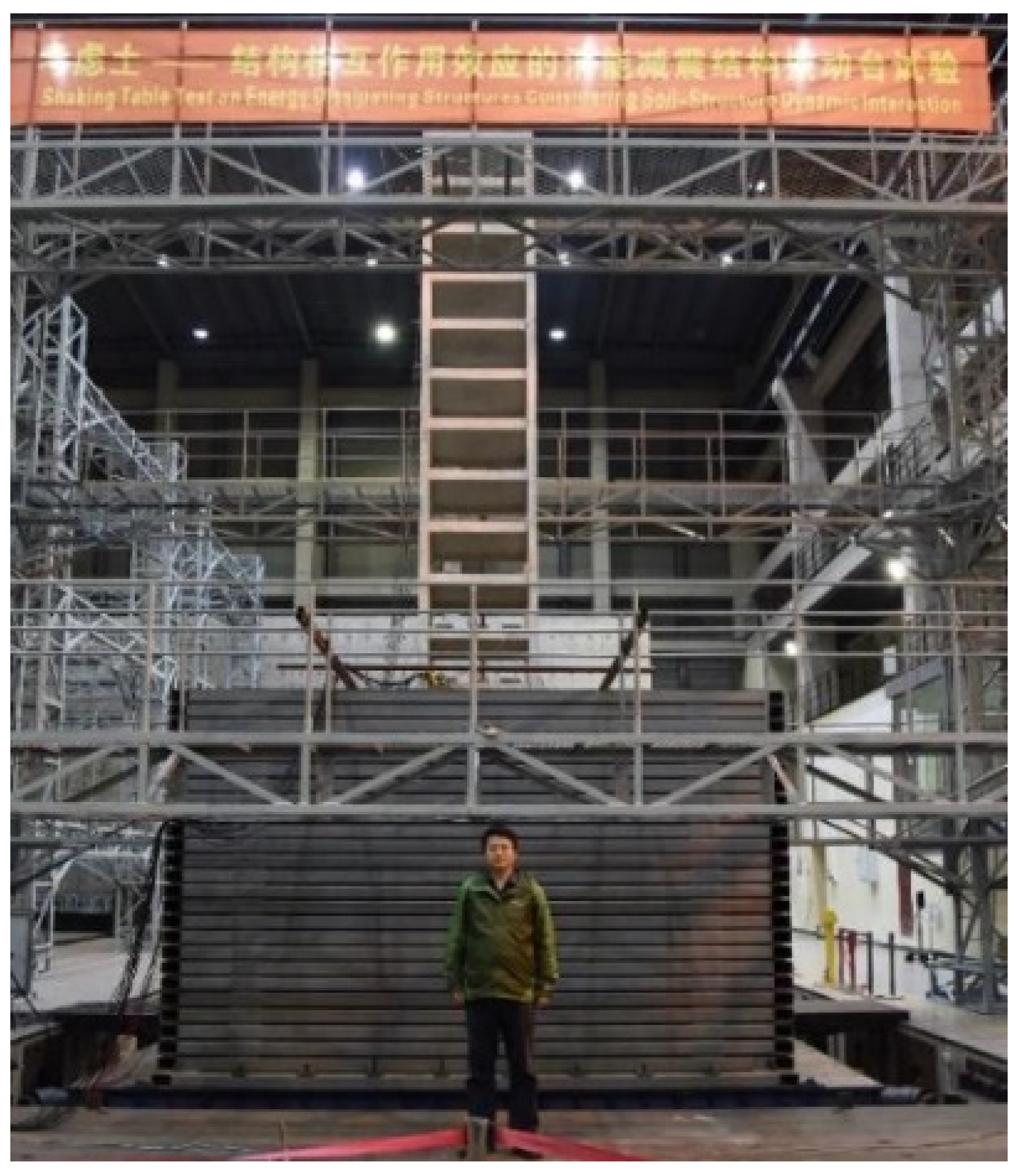
The essence of SSI lies in understanding how the flexible foundation medium alters the dynamic behavior of structures, drawing upon principles from geotechnical engineering, structural dynamics, and earthquake engineering. Extensive research has been dedicated to SSI, employing refined finite element models and analytical approaches [25,26]. Experimental validation through field and laboratory testing, particularly shaking table tests, is crucial for verifying numerical and analytical SSI models [27,28,29,30,31]. The existing research has significantly advanced our understanding of SSI; however, a persistent challenge remains in accurately incorporating SSI effects into system parameter identification for SHM. Traditional approaches often simplify input as ground-level acceleration and output as superstructure response, neglecting the complex, multi-directional foundation motions induced by SSI [32,33]. This simplification limits the accuracy of modal parameter identification, especially for structures on compliant soils.

Therefore, accurate modal parameter identification that explicitly accounts for SSI is of paramount importance for reliable SHM and seismic safety assessment of civil infrastructure. This paper seeks to address this critical need by developing and experimentally validating a novel SABO-VMD optimized approach for enhanced SHM of frame structures subjected to seismic loading, with careful consideration of the intricate effects of SSI. A key contribution of this methodology lies in the application of SABO-VMD for SSI-aware modal parameter identification, potentially enabling more accurate and robust damage assessment in seismically vulnerable regions. Experimental validation suggests the potential of the proposed approach in quantifying energy entropy indicators and analyzing SSI effects, offering a promising avenue for more reliable monitoring in earthquake-prone regions.

2. VMD Method and Principles

VMD is a signal-processing technique that decomposes a multicomponent signal into a discrete number of band-limited intrinsic mode functions (IMFs). In VMD, the core principle is to find modes that minimize the sum of the bandwidths of each mode around their respective center frequencies. This minimization process is formulated as a constrained variational problem. Consequently, the VMD algorithm can be delineated into two key stages: the construction of the variational problem and its subsequent solution.

(1)

Construction of the variational problem:

In contrast to Empirical Mode Decomposition (EMD), VMD defines each mode as an amplitude-modulated and frequency-modulated (AM-FM) signal, expressed as follows:

$$u_k\left(t\right)=A_k\left(t\right)\cos {\varnothing }_k\left(t\right)$$

(1)

where ${\mathit{A}}_{\mathit{k}}\left(\mathit{t}\right)$ represents the envelope amplitude of signal ${\mathit{u}}_{\mathit{k}}\left(\mathit{t}\right)$, and ${\varnothing }_{\mathit{k}}\left(\mathit{t}\right)$ indicates the phase of the signal.

To estimate the bandwidth of each mode, the analytic signal is employed. By applying the Hilbert transform to each mode, $u_k\left(t\right)$, we obtain its analytic signal representation, which yields a one-sided spectrum. The analytic signal of the k-th mode, denoted as $u_k\left(t\right)$, is given by the following:

By applying the Hilbert transform to the signal, the analytic signals of the K modal components can be extracted, thereby obtaining the one-sided spectrum for each component.

$$\left[\delta \left(t\right)+{\displaystyle \frac{j}{nt}}\right]u_k\left(t\right)$$

where $\delta \left(t\right)$ represents the impulse response, and H(t) is the Hilbert transform operator.

For each modal analytic signal, the center frequency, $e^{-j{\omega }_k^t}$, is estimated in advance, and the respective modal spectrum is adjusted to align with the corresponding fundamental frequency band based on this center frequency:

$$\left\{\left[\delta \left(t\right)+{\displaystyle \frac{j}{nt}}\right]u_k\left(t\right)\right\}{e}^{-j{\omega }_k^t}$$

The squared gradient (L²) of the aforementioned demodulated signals is computed to estimate the bandwidth of each modal signal. A constrained variational model is employed for this purpose:

$$\left\{\begin{array}{c}\underset{\left\{u_k\right\},\left\{{\omega }_k\right\}}{\min }\left\{{\sum }_k{‖d_t\left[\left(\delta \left(t\right)+{\displaystyle \frac{j}{nt}}\right)·u_k\left(t\right)\right]e^{-j{\omega }_k^t}‖}_2^2\right\}\\ s·t·{\sum }_k{u}_k=f\end{array}\right.$$

(2)

Solution of the variational problem:

To convert the constrained variational problem into an unconstrained one, a quadratic penalty factor and Lagrange multipliers are introduced, resulting in the formulation of an extended Lagrange expression:

$$L\left(\left\{u_k\right\},\left\{{\omega }_k\right\},\lambda \right)=\alpha \sum _{K=1}^K‖{\left\{\left[\left(\delta \left(t\right)+{\displaystyle \frac{j}{nt}}\right)·u_k\left(t\right)\right]e^{-j{\omega }_k^t}\right\}‖}_2^2+‖{f\left(t\right)-{\sum }_{K=1}^K{u}_k\left(t\right)‖}_2^2+<\lambda \left(t\right),f\left(t\right)-\sum _{K-1}^K{u}_k\left(t\right)>$$

(2)

By employing the iterative algorithm described above to compute the variational model, K modal components are obtained in the frequency domain. The Fourier transform is then applied to retrieve the K modal components in the time domain, which can be further processed based on the signal characteristics of each modal component.

3. Parameter Sensitivity Analysis in VMD Decomposition

In the preceding section outlining the VMD algorithm, it was noted that the algorithm involves four key parameters: the number of intrinsic modal components, K; the penalty factor, α; the noise tolerance, λ; and the accuracy criterion, ε. In most applications, the noise tolerance (λ) and the accuracy criterion (ε) have a minor impact on the VMD decomposition results, typically set to default values of λ = 0 and ε = 1.0 × 10⁻⁷. Therefore, this study primarily explores the influence of parameters K and α on the decomposition results, using specific amplitude modulation and frequency modulation signals for simulation experiments:

$$x\left(t\right)=\left(2+\cos \left(29\prod t\right)\right)\left[5\cos \left(100\prod t+2\cos \left(30\prod t\right)\right)\right]{10}^{-7}$$

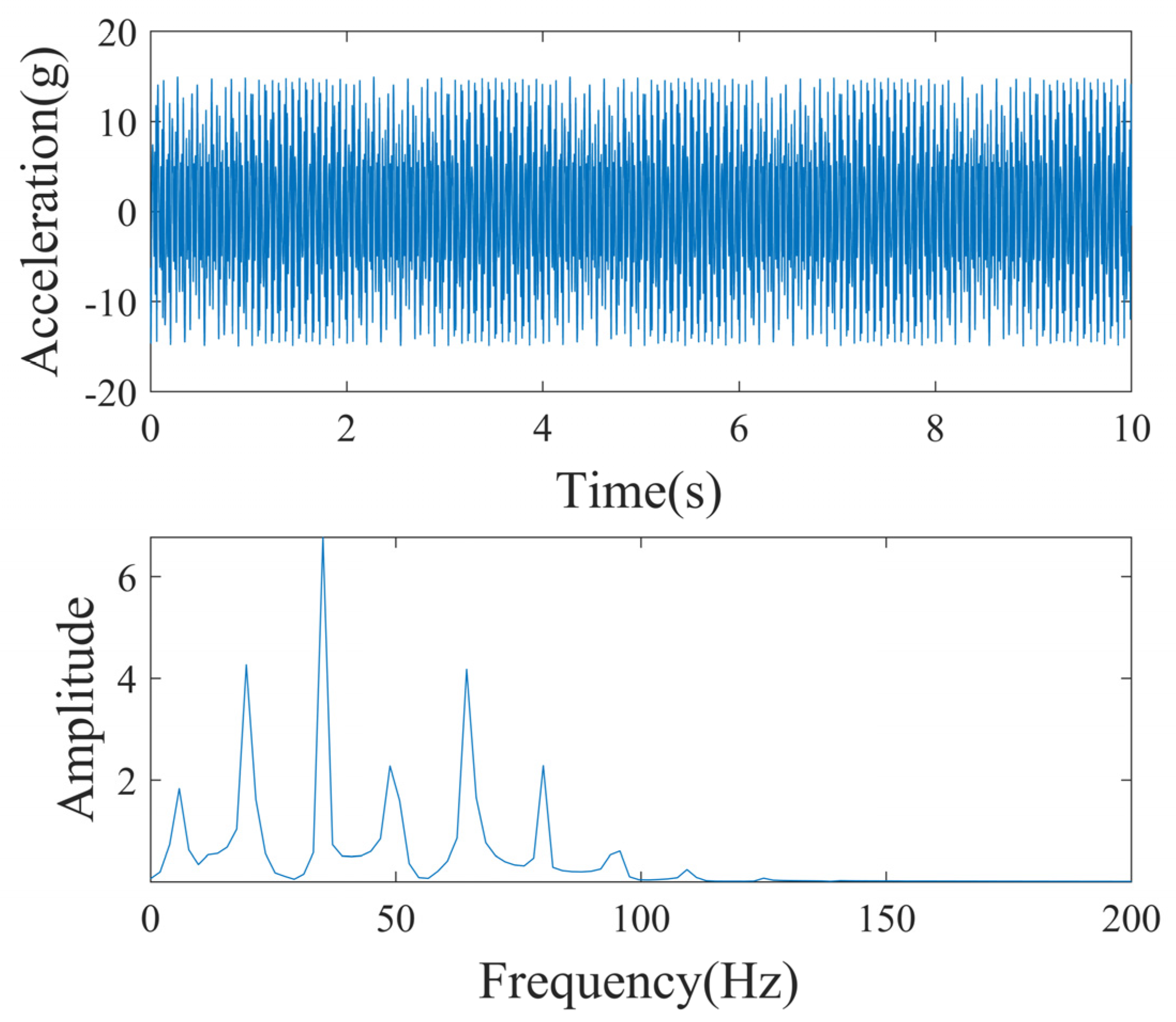
The sampling frequency, Fs, is 1000 Hz. As shown in Figure 1, the simulated signal mainly contains five frequency components: 20 Hz, 35 Hz, 50 Hz, 65 Hz, and 80 Hz.

3.1. Influence of the Number of Modes, K

The selection of the number of modes, K, in VMD is crucial. Often determined empirically, an inappropriate choice of K can lead to either under-decomposition or over-decomposition. Under-decomposition, resulting from an insufficient K, may lead to incomplete signal separation and failure to extract critical information. Conversely, over-decomposition, caused by an excessively large K, can result in mode mixing and spectral redundancy, leading to spurious modes and overlapping center frequencies.

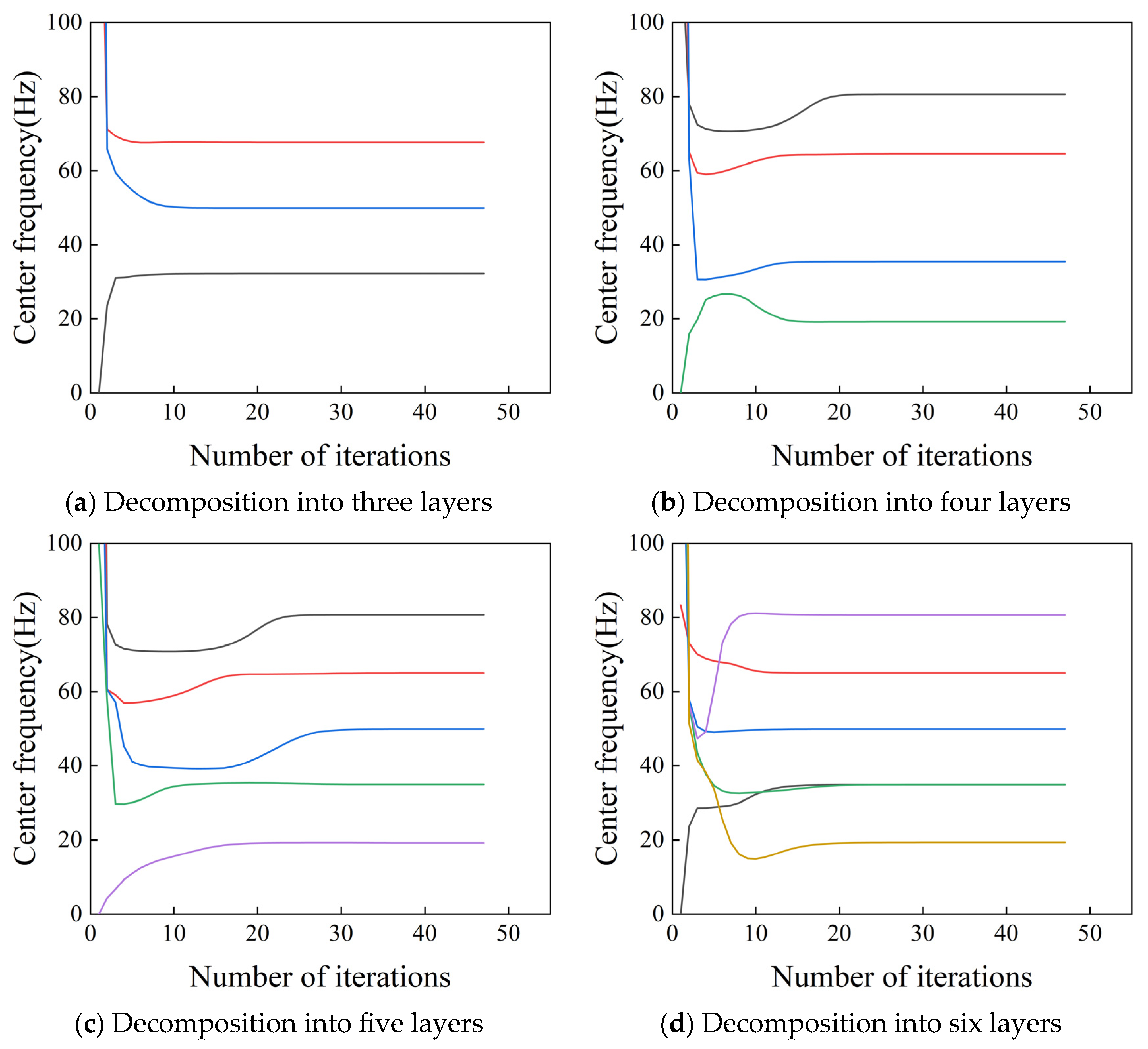
To investigate the effect of K, we set the penalty factor, α, to 2000 and performed VMD with K values of 3, 4, 5, and 6. The resulting center frequency trajectories are shown in Figure 2, revealing a significant impact of K on the decomposition results. With K = 3 and K = 4, the primary frequency components are not fully resolved, indicating under-decomposition. At K = 5, all intended frequency components are successfully extracted, suggesting an appropriate selection of K. However, when K = 6, the 20 Hz component is missed, and spurious components emerge around 30 Hz, signifying over-decomposition and mode splitting.

3.2. Influence of the Penalty Factor α

The penalty factor, α, directly governs the bandwidth of the decomposed modes. A smaller α allows for larger bandwidths, increasing the potential for spectral overlap and mode mixing. Conversely, a larger α restricts the bandwidths, potentially causing important signal components to be excluded from the extracted modes, leading to incomplete decomposition.

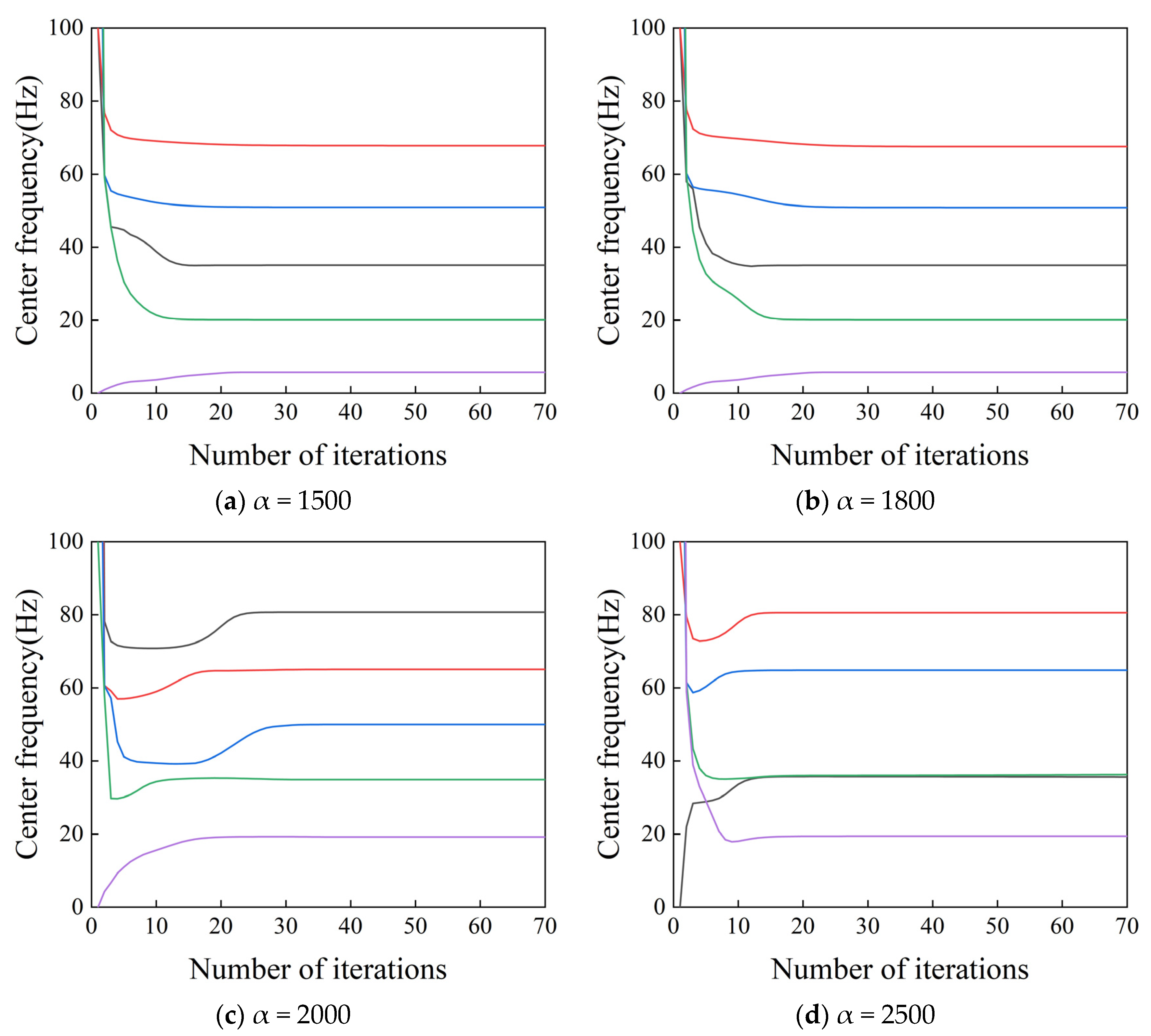
To examine the influence of α, we fix the number of modes at K = 5 and vary α through values of 1500, 1800, 2000, and 2500 for VMD decomposition. The resulting center frequency trajectories are presented in Figure 3.

Figure 3 demonstrates the non-monotonic effect of α on the decomposition results when K is held constant. At α = 1500, spurious components appear near 5 Hz, and the 65 Hz component is not effectively extracted. For α = 1800, both the 65 Hz and 80 Hz components are missed, indicating inadequate decomposition of the original signal’s frequency content. At α = 2000, all primary frequency components are successfully decomposed. However, when α = 2500, the 50 Hz component is not extracted, leading to mode mixing and spectral leakage.

4. Adaptive VMD Parameter Optimization Using Subtractive Average-Based Optimizer (SABO)

As demonstrated in the preceding analysis, the performance of VMD is significantly influenced by the selection of the number of modes (K) and the penalty factor (α). Different combinations of these parameters can yield substantially varying decomposition results. Furthermore, the conventional approach of empirically determining K and α through manual tuning is often subjective, time-consuming, and computationally expensive, making it challenging to consistently identify the optimal parameter configuration. To address these limitations, this paper proposes an intelligent optimization strategy employing the Subtractive Average-Based Optimizer (SABO) algorithm to adaptively determine the optimal K and α parameters for VMD. Sample entropy is selected as the fitness function for the SABO algorithm. This approach not only automates the parameter tuning process, eliminating tedious manual adjustments, but also enhances the accuracy and efficiency of parameter selection, leading to improved VMD performance.

4.1. Subtractive SABO Method

(1)

Population initialization:

Every optimization problem is defined within a solution space, often referred to as the search space. This space is a multi-dimensional domain, where the dimensionality corresponds to the number of decision variables in the optimization problem. Optimization algorithms explore this search space through a population of search agents, each representing a potential solution. The position of each search agent within the search space encodes the values of the decision variables. Mathematically, the population of search agents can be represented as a matrix, as shown in Equation (3). Equation (4) randomly initializes the search agents at the primary location in the search space.

$$X={\left[\begin{array}{c}{X}_1\\ ⋮\\ X_i\\ ⋮\\ X_N\end{array}\right]}_{N\times m}={\left[\begin{array}{ccccc}{x}_{\mathrm{1,1}}& \dots & x_{1,j}& \dots & x_{1,m}\\ ⋮& \ddots & ⋮& ⋰& ⋮\\ x_{i,1}& \dots & x_{i,j}& \dots & x_{i,m}\\ ⋮& ⋰& ⋮& \ddots & ⋮\\ x_{N,1}& \dots & x_{N,j}& \dots & x_{N,m}\end{array}\right]}_{N\times m}$$

(3)

$$x_{i,j}=l{b}_j+r_{i,j}·\left(u{b}_j-l{b}_j\right),i=1,\dots ,N,j=1,\dots ,m$$

(4)

where $x_{i,j}$ represents the generated individuals; ${ub}_j$ and ${lb}_j$ are the upper and lower boundaries of the population range, respectively; and rand denotes a random number between 0 and 1.

(2)

Objective function evaluation:

Each search agent’s position defines a set of decision variable values. The objective function, also known as a fitness function, evaluates the quality of each solution. The objective function quantifies how well each search agent performs with its current set of decision variables. The results of evaluating the objective function for all search agents are stored in a vector, denoted as $\overrightarrow{F}$, as shown in Equation (5):

$$\overrightarrow{F}={\left[\begin{array}{c}{F}_1\\ ⋮\\ F_i\\ ⋮\\ F_N\end{array}\right]}_{N\times 1}={\left[\begin{array}{c}F\left(X_1\right)\\ ⋮\\ F\left(X_i\right)\\ ⋮\\ F\left(X_N\right)\end{array}\right]}_{N\times 1}$$

(5)

where $\overrightarrow{F}$ is the vector of objective function values. $F_i$ represents the objective function value calculated for the i-th search agent. A higher (or lower, depending on the optimization problem—maximization or minimization) objective function value indicates a better solution. The SABO algorithm iteratively updates the positions of search agents in the search space, continuously seeking to improve the objective function value.

(3)

Mathematical model of SABO search mechanism:

The SABO algorithm updates the position of each search agent based on the subtractive average strategy. The new position of the i-th search agent, $x_i^{new}$, is calculated using Equation (6):

$$x_i^{new}=x_i+\overrightarrow{r_i}\times {\displaystyle \frac{1}{N}}{\sum }_{j=1}^N\left(X_i-V{X}_j\right),i=\mathrm{1,2}\dots ,N;j=\mathrm{1,2}\dots ,N$$

(6)

where N is the population size, and $\overrightarrow{r_i}$ is a vector with dimension m, with each component drawn from the normal distribution within the interval [0, 1]. The term $X_i-V{X}_j$ represents the vector difference between the i-th search agent and a scaled version of the j-th search agent (where V is a scaling factor, assumed to be 1 here for simplicity but could be a parameter). This subtraction and averaging process forms the core search mechanism of SABO.

If the proposed new location increases the value of the objective function (improving the optimization performance), we accept the location as the new location of the search agent, as shown in Equation (7).

$$x_i=\left\{\begin{array}{c}{x}_i^{new},F_i^{new}<F_i;\hfill \\ x_i, eles,\hfill \end{array}\right.$$

(7)

where $F_i$ and $F_i^{new}$ represent the objective function values of search agents $X_i$ and $x_i^{new}$, respectively.

After updating all search agents, the algorithm completes its first iteration. Subsequently, the algorithm moves to the next iteration based on the evaluation of the new location and the calculation of the objective function. In each iteration, the best search agent is stored as the optimal candidate solution from that iteration.

4.2. Sample Entropy as Fitness Function

Entropy is a fundamental concept in information theory and signal processing, quantifying the degree of randomness or uncertainty in a system or signal. In time-series analysis, entropy measures, such as approximate entropy, energy entropy, and sample entropy, are valuable tools for characterizing signal complexity and irregularity [34,35]. Sample entropy, a nonlinear dynamic measure, is particularly well-suited for quantifying the regularity and unpredictability of fluctuations in a time series. Lower sample entropy values indicate higher signal regularity, while higher values suggest greater irregularity.

In this study, we employ sample entropy as the fitness function for SABO-VMD. The rationale is that minimizing the sample entropy of the decomposed modes can lead to more regular and physically meaningful IMFs, thereby optimizing the VMD decomposition. The calculation of sample entropy for a time series X = {x(1), x(2), …, x(N)} of length N is performed through the following steps:

Step1: Phase space reconstruction. Construct m-dimensional vectors from the time series X:

$$X\left(i\right)=\left\{x\left(i\right),x\left(i+1\right), \dots ,x\left(i+m-1\right)\right\}, i = 1, 2,\dots ,N--,m+1$$

(8)

where m is the embedding dimension.

Step 2: Distance calculation. Define the distance d[X(i), X(j)] between vectors X(i) and X(j) (i ≠ j) as the maximum absolute difference between their corresponding elements:

$$\mathrm{d}\left[X\left(i\right),X\left(j\right)\right]=\underset{k\in \left(0,m-1\right)}{\max }\left|x\left(i+k\right)-x\left(j+k\right)\right|$$

(9)

Step 3: Similarity count. Given a tolerance threshold r (r > 0), count the number of vector pairs (X(i), X(j)) for which d[X(i), X(j)] < r. Calculate the ratio of this count to the total number of possible pairs, (N − m):

$$B_i^m\left(r\right)={\displaystyle \frac{1}{N-m}}\mathrm{n}\mathrm{u}\mathrm{m}\left\{\mathrm{d}\left[X\left(i\right),X\left(j\right)\right]<r\right\}$$

(10)

Step 4: Average Similarity. Calculate the average similarity measure $B^m\left(r\right)$ across all vectors X(i):

$$B^m\left(r\right)={\displaystyle \frac{1}{N-m+1}}\sum _{i=1}^{N-m+1}{B}_i^m\left(r\right)$$

(11)

Step 5: Repeat for increased dimension. Increment the embedding dimension to m + 1 and repeat Steps 1 to 4 to calculate $B^{m+1}\left(r\right)$.

Step 6: The sample entropy is estimated as follows:

$$\mathrm{S}\mathrm{a}\mathrm{m}\mathrm{p}\mathrm{E}\mathrm{n}\left(m,r\right)=\underset{N\to \infty }{\lim }\left\{-\ln \left[{\displaystyle \frac{B^{m+1}\left(r\right)}{B^m\left(r\right)}}\right]\right\}$$

(12)

However, in practice, N cannot reach theoretical infinity and has a finite limit, so the sample entropy is estimated as follows:

$$\mathrm{S}\mathrm{a}\mathrm{m}\mathrm{p}\mathrm{E}\mathrm{n}\left(m,r,N\right)=-\ln \left[{\displaystyle \frac{B^{m+1}\left(r\right)}{B^m\left(r\right)}}\right]$$

(13)

Sample entropy calculation excludes self-comparisons, enhancing computational accuracy and efficiency. Furthermore, sample entropy exhibits good consistency, meaning that for a given time series, the influence of parameters m and r on the entropy value is relatively stable. These properties make sample entropy a robust and suitable fitness function for optimizing VMD parameters using SABO.

4.3. SABO Parameter Selection for VMD Optimization

The performance of the SABO algorithm is influenced by its internal parameters, including population size (n), maximum number of iterations (D), and the range of optimization variables. Appropriate parameter settings are crucial for achieving effective optimization.

Population size (n): A small population size may limit the algorithm’s exploration capability, leading to premature convergence and entrapment in local optima. Conversely, an excessively large population can increase computational cost and slow down convergence.

Maximum number of iterations (D): Insufficient iterations may not allow for adequate exploration of the search space. Excessive iterations can lead to overfitting or diminishing returns in optimization progress.

Optimization variables: In this study, the optimization variables are the VMD parameters, K (number of modes) and α (penalty factor). The algorithm needs to effectively search the two-dimensional parameter space defined by K and α.

To optimize the VMD parameters K and α, we utilize a dataset from a 12-story frame structure. The SABO algorithm is configured with the parameter settings summarized in

Table 1. SABO-VMD parameter settings.

n	D	$\mathit{u}{\mathit{b}}_{\mathit{j}}$	$\mathit{l}{\mathit{b}}_{\mathit{j}}$	Number of Optimized Variables
25	20	[100, 3]	[2500, 10]	2

Note:$u{b}_j$ is the upper limit of the penalty factor and K, while $l{b}_j$ is the lower limit of the penalty factor and K.

.

4.4. SABO-VMD Parameter Optimization Procedure and Results

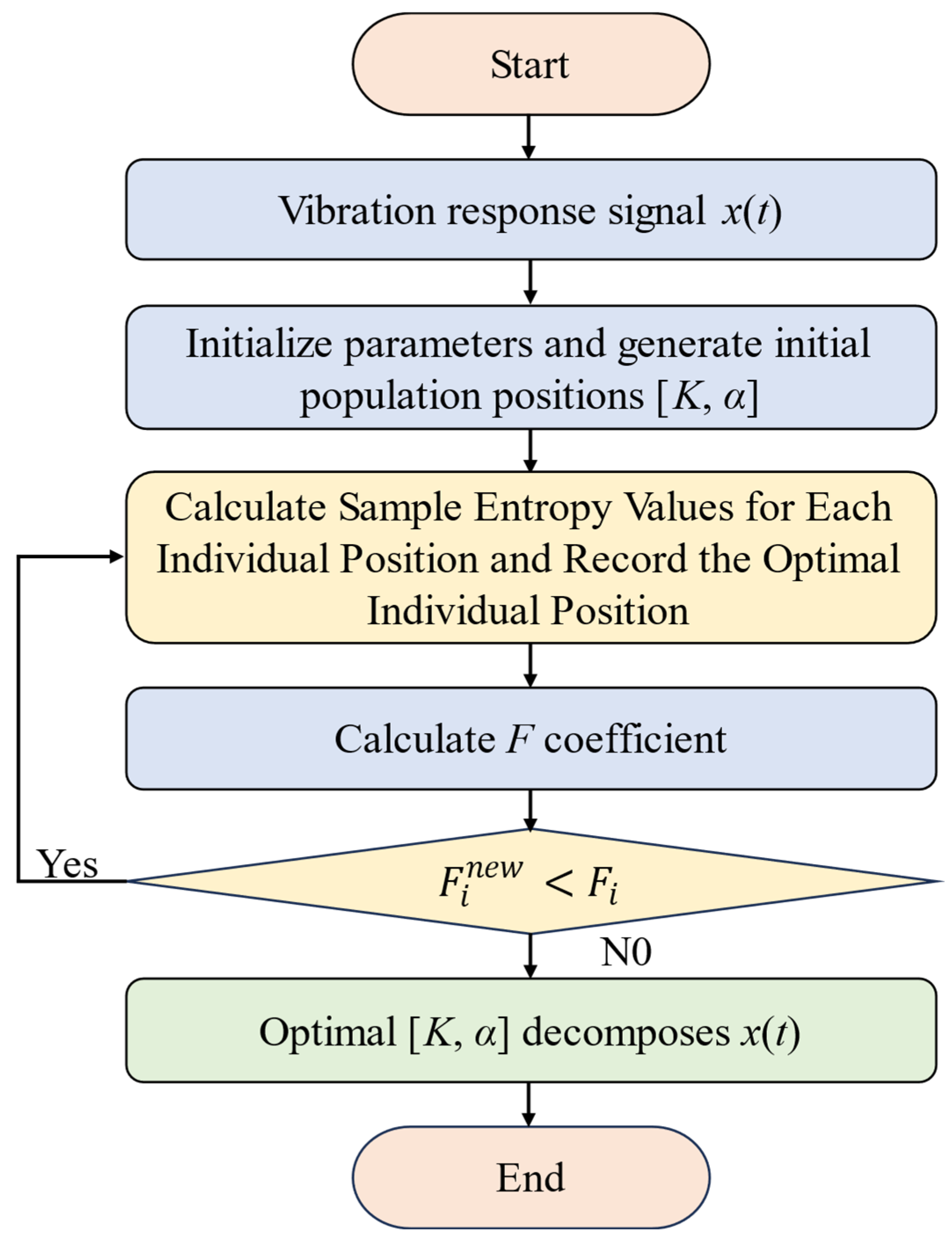
The parameter optimization steps of SABO-VMD are illustrated in Figure 4.

To demonstrate the effectiveness of SABO-VMD, we applied it to optimize the VMD parameters using experimental vibration data from the Case Western Reserve University (CWRU) bearing dataset, specifically using the 0.007 mm diameter rolling element fault data. Sample entropy was employed as the objective function to be minimized. The SABO parameters were set as follows: n = 25, D = 20, upper bounds $u{b}_j$ = [2500, 10], and lower bounds $l{b}_j$ = [100, 3].

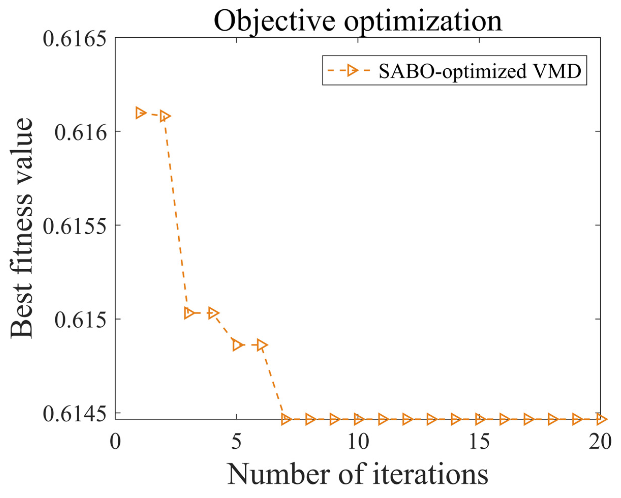
The optimization process was run for 20 iterations. Figure 5 shows the convergence curve of the fitness function (sample entropy) during the SABO optimization. It is observed that the fitness value reaches an optimal state after approximately 10 iterations, converging to a minimum sample entropy value of 0.6144. Based on the SABO optimization, the optimal VMD parameters were determined to be K = 10 and α = 825.

5. Experimental Validation and Comparative Results

To validate the efficacy of the proposed SABO-VMD approach in decomposing structural response data, this section presents a comparative analysis using experimental data obtained from a 12-story frame structure shaking table test. The performance of SABO-VMD is benchmarked against two established methods: EMD and the original VMD with manually tuned parameters. Furthermore, SABO-VMD is applied to identify structural dynamic characteristics of the 12-story frame under varying damage conditions, demonstrating its capability for structural health monitoring.

5.1. Introduction to the Shaking Table Test

The parameter optimization and validation presented in this paper are based on data from a comprehensive shaking table test conducted at Tongji University on a 12-story reinforced concrete frame structure, considering SSI [29]. The experimental design incorporated two model configurations: one accounting for soil–structure interaction (PS model) and another with a fixed-base boundary condition (RS model). This dual-model approach allowed for detailed observation of the seismic response characteristics and dynamic behavior of the superstructure, pile foundation, and surrounding soil under simulated earthquake loading. The physical model of the test structure is illustrated in Figure 6. The superstructure was a bidirectional, single-bay, 12-story reinforced concrete frame, designed according to relevant structural engineering codes [28].

To capture the dynamic response of the superstructure, a suite of instrumentation was deployed, including accelerometers and displacement transducers strategically placed on each floor. Detailed information regarding the instrumentation layout and measurement point locations for the shaking table tests is available in Reference [27].

5.2. Comparison of Decomposition Methods: SABO-VMD, VMD, and EMD

To rigorously evaluate the performance of SABO-VMD in extracting meaningful time–frequency information from structural vibration signals, we compared its decomposition results with those obtained using EMD and the original VMD. Acceleration signals recorded at the base of the structure under seismic loading condition SJ1 (specify SJ1 condition—e.g., low-intensity earthquake) were analyzed using all three methods. The time–frequency representation of the original, unprocessed acceleration signal is shown in Figure 7. The decomposed modes obtained by EMD, original VMD, and SABO-VMD are presented in Figure 8, Figure 9, and Figure 10, respectively.

A visual comparison of Figure 8, Figure 9 and Figure 10 clearly reveals the distinct performance characteristics of each decomposition method. Figure 8 displays the time–frequency representation of the intrinsic mode functions (IMFs) obtained from EMD. EMD decomposed the signal into seven IMFs. However, the time-domain plots exhibit evidence of spurious modes, and the frequency-domain representations show chaotic spectral amplitudes and significant mode mixing. The inherent limitations of EMD, such as mode mixing and spurious mode generation, hinder the clear identification of individual frequency components and impede accurate feature extraction. Therefore, in practical applications, it is essential to carefully evaluate the results of EMD decomposition and consider combining it with other signal-processing methods to enhance the accuracy and reliability of feature extraction.

Figure 9 presents the modes decomposed by the original VMD, using manually selected parameters, resulting in eight modes. Compared to EMD, VMD effectively mitigates spurious mode generation and yields more coherent and interpretable modes, highlighting the inherent advantages of the variational mode decomposition framework. However, despite the improvements over EMD, the VMD decomposition with manually tuned parameters still exhibits noticeable mode mixing, likely due to the sub-optimal parameter selection. Manually searching for the optimal parameter combination is a challenging and subjective process. It is difficult to ensure the validity and reliability of the decomposition results.

In stark contrast, Figure 10 demonstrates the superior performance of the proposed SABO-VMD method. SABO-VMD automatically optimizes the VMD parameters (K and α) using sample entropy as the fitness function, eliminating the subjectivity and uncertainty associated with manual parameter tuning. The resulting decomposition exhibits significantly reduced mode mixing, yielding more distinct and reliable mode components with clearer time–frequency representations. SABO-VMD effectively extracts physically meaningful modes that accurately represent the underlying dynamics of the structural vibration signal. Through this method, researchers are able to better understand and analyze the characteristics of vibration signals, providing a reliable foundation for subsequent engineering applications.

5.3. Structural Health Identification and Natural Frequency Analysis

Natural frequencies are fundamental dynamic characteristics of structures and serve as critical indicators of structural health. Changes in natural frequencies can signify structural damage or degradation. To demonstrate the application of SABO-VMD for structural health monitoring, we decomposed vibration acceleration signals recorded at the base of the 12-story frame structure under varying seismic intensity conditions using SABO-VMD. The time–frequency representations of the decomposed modes for conditions SJ1 and SJ5 are shown in Figure 11 and Figure 12, respectively.

Observations from Figure 11 and Figure 12 indicate a clear trend: as the severity of structural damage increases (from SJ1 to SJ5), the waveforms of the characteristic modes become progressively more complex and irregular, and the estimated natural frequencies exhibit a decreasing trend. This frequency reduction is consistent with the expected behavior of structures experiencing stiffness degradation due to damage. Figure 11 presents the acceleration signals and frequency responses under different damage states. As the level of damage increases, the amplitude and shape of the waveforms undergo significant changes. Figure 12 similarly displays the acceleration signals and frequency responses under different damage states, but in this figure, the level of damage is more severe.

Table 2. Results of intrinsic frequency extraction.

Condition	Intrinsic Frequency/Hz
	First Order	Second Order	Third Order	Fourth Order
SJ1	5.40	15.14	17.93	26.98
SJ3	5.386	12.07	15.72	25.63
SJ4	5.36	12.05	15.49	25.59
SJ5	5.37	10.39	114.57	24.23

summarizes the primary mode natural frequencies. From Table 2, a clear correlation between structural damage and natural frequency reduction is evident. The highest natural frequency is observed under condition SJ1 (healthy state). While the first-order frequency under condition SJ3 is close to that of SJ1, a slight reduction is observed, indicating minor structural damage. Under condition SJ4, the natural frequency further decreases, suggesting moderate damage affecting the structural dynamic characteristics. Notably, under condition SJ5, the natural frequency exhibits a significant deviation from the healthy state (SJ1), indicating substantial structural health deterioration. These results demonstrate the sensitivity of SABO-VMD-extracted natural frequencies to structural damage and its potential for quantitative structural health assessment.

6. Damage State Characterization

Building upon the preceding discussion, the VMD parameters are iteratively optimized using the SABO algorithm to enhance decomposition performance. Structural damage induces a redistribution of energy within vibration signals. Energy entropy serves as an effective metric for evaluating the energy distribution in complex systems and provides insights into structural health. In this study, we employ the SABO-VMD algorithm to decompose vibration signals and extract energy information from each IMF component. Subsequently, we analyze the structural damage state through statistical analysis of the energy entropy.

6.1. Statistical Energy Entropy Based on SABO-VMD

SABO-VMD decomposes the vibration signal into K IMF components, with the energy values of each component represented as E₁, E₂, …, E_k. The total energy, E, is the sum of these individual component energies. Since the IMF components convey information across different frequency ranges, the set E = {E₁, E₂, …, E_k} illustrates the energy distribution characteristics of the structural vibration signal in the frequency domain. Accordingly, the energy entropy of the SABO-VMD is defined as follows.

$$H=-\sum _{i=1}^k{p}_i{\log }_2{p}_i$$

(14)

where p_i (p_i = E_i/E) denotes the proportion of the energy, E_i, of the i-th IMF component relative to the total energy, E.

To validate the effectiveness of SABO-VMD in structural health assessment, we decomposed acceleration signals under SJ wave excitation for various damage conditions of a 12-story frame structure with even-numbered floors using SABO-VMD. Energy entropy was then calculated for statistical analysis and mapping. For comparative purposes, we also present energy entropy results derived from EMD.

Figure 13a reveals a decreasing trend in entropy values with increasing damage severity. The energy entropy values for condition SJ3 are similar to those for SJ2, which aligns with shaking table test observations indicating no cracking in the upper structure for the first ten conditions. Condition SJ4 exhibits moderate entropy values, while SJ5, representing the most severe damage, shows the lowest entropy values. Furthermore, entropy values for the fourth and tenth floors of the damaged structure are comparatively lower than those of other floors. This may be attributed to weaker nodes at these floors, leading to a more pronounced structural response. Thus, targeted strengthening measures should be considered at these locations during frame structure design.

Figure 13b shows the statistical results for EMD energy entropy. The differences in EMD energy entropy across damage conditions are minimal, suggesting that EMD energy entropy may not accurately reflect the degree of structural damage. Conversely, energy entropy derived from SABO-VMD provides a more accurate and sensitive assessment of structural damage levels.

6.2. State Analysis of Energy Entropy Under SSI System

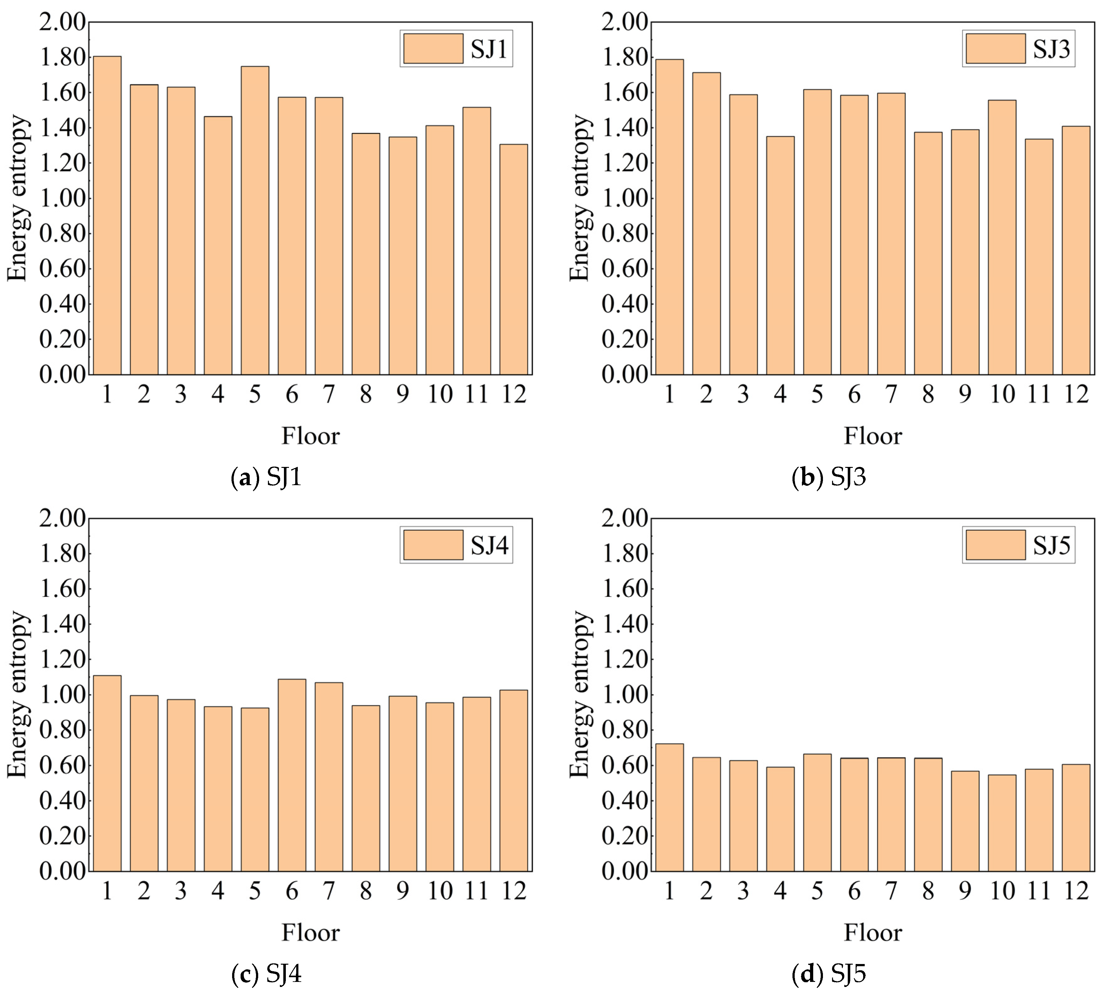
To further validate the effectiveness of SABO-VMD energy entropy in structural damage assessment, VMD parameters were optimized, and decomposition was performed for each floor under each damage condition to calculate energy entropy. The statistical results are presented in Figure 14.

As shown in Figure 14, the fluctuation range of energy entropy values across different floors under the same working conditions is relatively small, indicating the stability of SABO-VMD energy entropy in practical applications. Under undamaged conditions, the distribution of structural vibration signals is more uniform and uncertain, leading to higher entropy values.

Figure 14 shows that for SJ1 and SJ3 (undamaged conditions), entropy values are above 1, typically ranging from 1.2 to 1.8. In SJ4, entropy values are generally below 1.1, with even lower values for intermediate floors (3–5 and 8–11), suggesting potential weak links in the middle sections. Finally, in SJ5, energy entropy reaches its minimum, indicating that all floors have entered a damage state with visible structural degradation.

SABO-VMD energy entropy of the 12-story frame structure reveals that middle floors experience more severe damage. Under eight damage conditions, entropy values for upper (9–11) and lower (2–4) floors are lower than those of intermediate floors. Therefore, targeted reinforcement strategies should be considered for these floor regions during frame structure design.

6.3. Comparative Analysis of Energy Entropy Under SSI System and Fixed-Base Foundation

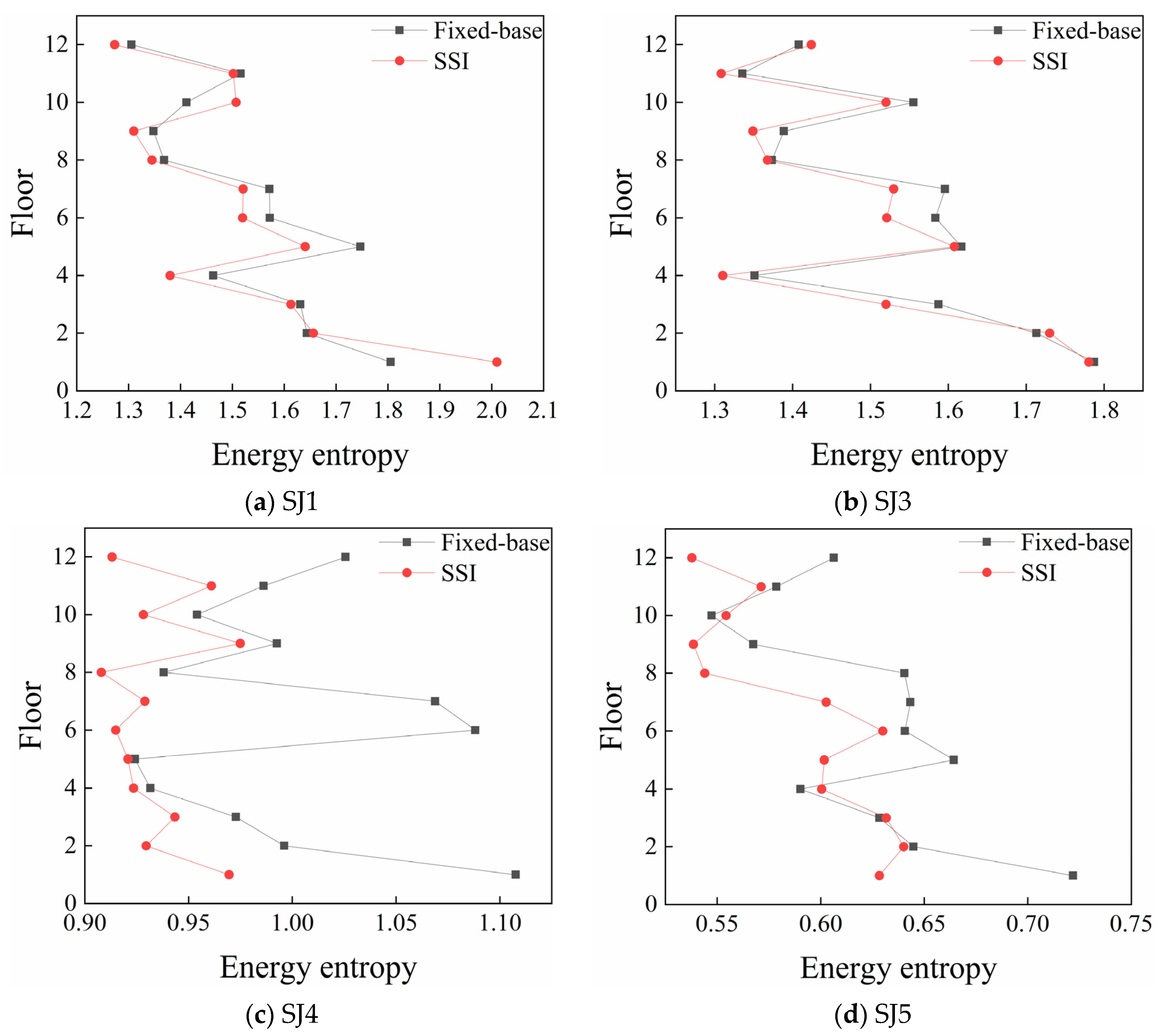
To investigate the influence of SSI on the frame structure, Figure 15 compares floor energy entropy values (SABO-VMD) for the 12-story frame structure under fixed-base and SSI conditions across various damage states. As the structure remains largely undamaged in the first ten conditions, only SJ1 and SJ3 are selected for comparative statistical analysis.

Figure 15 shows that for the fixed-base structure, energy entropy values for SJ1 and SJ3 are high, indicating an undamaged state up to SJ3. Under SJ4 condition, entropy values drop below 1, fluctuating between 0.9 and 1, signaling a transition to light damage. Under the SJ5 condition, energy entropy further decreases to between 0.55 and 0.65. At this point, entropy values are nearly half of those under the undamaged state, indicating that all floors have entered a damage state with visible structural degradation.

For the fixed-base foundation, intermediate floors, specifically floors 2–6 and 9–11, exhibit lower entropy values compared to others. This suggests weaker nodal connections in these intermediate layers, resulting in more pronounced seismic responses. This phenomenon may be related to the overall stiffness distribution of the structure, with the middle floors being more susceptible to deformation.

Compared to the fixed-foundation scenario, considering soil–structure interaction (SSI) generally results in higher energy entropy values under the same damage conditions, indicating that SSI may alter the overall dynamic response of the structure to resemble the undamaged state more closely. However, for the intermediate weak floors, SSI sometimes leads to decreased energy entropy values, implying a potential damping effect provided by soil–structure interaction. Specifically, under SJ5 operational conditions, the energy entropy for floors 1–8, considering SSI, ranges from approximately 0.53 to 0.63, while for the fixed foundation, it ranges from about 0.60 to 0.68. For the weaker floors (9–11), SSI slightly reduces the energy entropy, with ranges around 0.53 to 0.57, compared to approximately 0.58 to 0.63 for the fixed foundation. These results suggest that the impact of SSI varies across different floors, likely related to their position, stiffness, and connection mode with the ground.

Additionally, both fixed foundation and SSI foundation exhibit similar patterns of energy entropy variation, indicating that considering SSI does not alter the overall energy distribution along the height of the structure. However, based on the analysis of the SJ1-SJ5 operational conditions in Figure 15, a quantitative comparison of the energy entropy values at the fifth floor under SSI and fixed foundation conditions reveals that the inclusion of SSI reduces the damage degree of the structure by 8.1%. This result demonstrates that, for the 12-story frame structure analyzed in this study, soil–structure interaction plays a significant role in damping effects, effectively dissipating energy and thus mitigating the impact of seismic events on the structure’s response. It is important to note that this damping effect may be influenced by specific structural parameters, foundation characteristics, and the intensity of seismic motion; therefore, the influence of SSI might vary in other structures.

7. Conclusions

This study presents a novel approach for structural health monitoring, utilizing the SABO algorithm to optimize key parameters (K, number of modes; α, bandwidth control) within the VMD framework. The optimized SABO-VMD method was then applied to analyze seismic response data from a 12-story frame structure, considering both fixed-base and soil–structure interaction (SSI) conditions. The following conclusions are based on the analysis of acceleration signals from different floors and the energy entropy calculated from the decomposed modes.

(1)

Superior time–frequency resolution: SABO-VMD exhibits superior time–frequency resolution compared to EMD and standard VMD, facilitating clearer identification of modal frequencies in structural response signals. This improvement stems from the SABO algorithm’s effective optimization of VMD parameters, resulting in more accurate separation of intrinsic mode functions (IMFs). This enhanced separation is crucial for precisely identifying subtle changes in structural dynamics, enabling early damage detection.

(2)

Effective damage detection: Applying SABO-VMD to structural base acceleration signals under various damage scenarios revealed a consistent trend: the identified natural frequencies decreased with increasing damage severity. This confirms the sensitivity of SABO-VMD to structural changes and validates its effectiveness as a damage detection tool. The magnitude of the frequency shift serves as a direct indicator of the extent of structural degradation, providing a reliable and efficient means for assessing structural integrity and preventing catastrophic failures.

(3)

Impact of soil–structure interaction (SSI): This study highlights the significant impact of soil–structure interaction (SSI) on structural response. The higher energy entropy observed under SSI conditions suggests that SSI contributes to seismic damping, effectively dissipating energy and mitigating the impact of seismic events. This underscores the importance of considering SSI in accurate structural health assessments, particularly for structures on softer soils, leading to more realistic and cost-effective structural designs and retrofit strategies.

(4)

Limitations and future work: While the SABO-VMD method demonstrates promise, further research is needed to validate its generalizability across diverse structural types and under realistic environmental conditions. Future efforts will focus on integrating SABO-VMD with machine-learning techniques for automated damage detection and localization, enhancing its practical utility. Additionally, exploring and comparing alternative optimization algorithms within the VMD framework will drive continued performance improvements and broaden the method’s applicability in structural health monitoring.