Stress–Strain Prediction for Steam-Cured Steel Slag Fine Aggregate Concrete Based on Machine Learning Algorithms

Abstract

The utilization of steam-cured steel slag fine aggregate concrete (SC) faces challenges in accurately predicting its stress–strain relationship. The mechanical properties of steam-cured SC and its stress–strain relationship have been systematically investigated through combined tests and machine learning (ML) approaches. The results showed that steam curing at 50 °C greatly increased the peak stress and ductility of SC. Specimens, the steel slag fine aggregate (SA) content of which was 40% by volume, and which were subjected to steam curing at 50 °C, exhibited superior mechanical and deformation properties. The prediction performance of three ML models—random forest (RF), backpropagation neural network (BPNN), and support vector regression (SVR)—was compared based on the test data. The analysis results revealed that the RF model achieved optimal performance (R² = 1.00), whereas the SVR model underperformed overall. Through the transfer validation method, it was found that the BPNN model, after parameter optimization, demonstrated a superior generalization ability in cross-mix-proportion predictions. It exhibited satisfactory prediction stability for steam-cured SC with an untrained mix proportion. In contrast, the RF model tended to overestimate peak stress. The theoretical reference for realizing the comprehensive utilization of steel slag in precast concrete components has been provided.

1. Introduction

The superior mechanical properties, workability, and durability of concrete have made it widely applicable in various civil engineering fields, including roads, bridges, and buildings [1,2,3]. Similar to sustainable concrete [4] and recycled aggregate concrete [5], the replacement of natural aggregates with steel slag aggregates in concrete yields steel slag aggregate concrete, which can effectively improve the utilization rate of steel slag—a solid waste from the iron and steel industry—while conserving natural mineral resources and protecting the ecological environment [6,7,8].

In recent years, numerous researchers have focused increasingly on the mechanical properties [9,10,11] and stress–strain behaviors [12,13,14] of steel slag aggregate concrete. Guo et al. [9] investigated the static and dynamic compressive strength as well as the impact resistance of steel slag fine aggregate concrete with various replacement ratios (0%, 10%, 20%, 30%, and 40%), and recommended 20% as the optimal replacement ratio. Qasrawi et al. [10] investigated the influence of five substitution ratios (0%, 15%, 30%, 50%, and 100%) of steel slag fine aggregates on 25~45 MPa concrete, found positive impacts on both compressive and tensile strengths, and demonstrated that the proper content of steel slag fine aggregates to different concrete grades could significantly enhance their mechanical properties. Xue et al. [11] examined the macroscopic mechanical properties and microstructural characteristics of concrete and mortar with steel slag fine aggregates at 0%, 10%, 20%, and 30% replacement ratios, and observed improvements in compressive strength. Fu et al. [12] investigated the effects of a 10%~100% (in 20% increments) equal mass replacement of both coarse and fine aggregates with steel slag aggregates on the mechanical properties of concrete and derived a damage constitutive model that is highly consistent with the actual test results. Guo et al. [13] explored the impact of untreated steel slag replacements at various levels (0%, 10%, 20%, 30%, 40%, 60%, 80%, and 100%) for fine aggregates on the stress–strain behavior, compressive strength, and toughness of both normal-strength and high-strength concrete. Their [13] findings indicated that 20% and 80% steel slag contents improved both the compressive strength and toughness of the normal-strength specimens; the optimal compressive strength and toughness were exhibited by high-strength specimens with a 30% steel slag content; and steel slag incorporation generally enhanced the peak stress of normal-strength concrete. Chen et al. [14] examined the failure patterns, strength characteristics, deformation behavior, and failure criteria of steel slag aggregate concrete under multiaxial stress states and proposed the failure criterion derived from triaxial test data that accurately characterized the multiaxial strength properties of steel slag aggregate concrete.

However, the volume stability issues of steel slag limit its applications in construction engineering. Studies [15,16,17] have shown that autoclave or steam curing can effectively mitigate volume instability hazards caused by free calcium oxide (f-CaO) in steel slag. The long-term volume stability of steel slag fine aggregate concrete [18] also confirms the effectiveness of steam curing. Wang et al. [15] investigated the hydration characteristics of basic oxygen furnace (BOF) steel slag and found that increasing the curing temperature can accelerate the early hydration reaction of steel slag. Belhadj et al. [16] studied the hydration reaction rates of BOF slag pure paste specimens at 20, 40, 60, and 80 °C and found that increasing the curing temperature accelerated the hydration rate of BOF slag, but the carbonation of hydration products was observed when the temperature exceeded 60 °C. Feng et al. [19] investigated the compressive strength, failure mode, and stress–strain relationship of a steel slag aggregate concrete filled-in fiber-reinforced polymer tube (SSACFFT) with different steel slag coarse aggregate contents after steam curing (80 ± 2 °C, 95% humidity), and revealed that the SSACFFT has a higher stiffness than ordinary fiber-reinforced polymer tube concrete. They [19] also employed the three-dimensional laser scanning technique to examine the volume expansion effect of the SSACFFT during steam curing and found that steam curing accelerated the hydration reaction of steel slag in the concrete. Cai et al. [20] compared the performance of concrete under different steam curing systems and concluded that 50 °C steam curing is the most economical scheme for concrete precast structures to meet their mechanical properties. They [20] also considered this to be the optimal steam curing condition for precast concrete T-beams. Shao et al. [21] investigated the mechanical properties and microstructure of precast concrete under different steam curing temperatures. They [21] found that 60 °C and 80 °C accelerated the hydration of the cementitious materials but caused irreversible damage to the microstructure of the precast concrete. Additionally, they [21] observed that the delayed formation of ettringite occurred within 7 days after steam curing at temperatures above 60 °C, which can be detrimental to the volumetric stability of precast concrete. They [21] suggested that a temperature below 60 °C is more reasonable for steam curing. Duan et al. [22] used the steam curing system commonly employed in the production of precast beams for high-speed railways in China [23]—steam curing at 50 °C for concrete specimens. The mechanical properties of steam-cured steel slag aggregate concrete, as compared to standard-cured steel slag aggregate concrete, should be thoroughly investigated.

The compressive strength and stress–strain relationship of concrete are significant characteristics used to describe its mechanical properties and are important indicators for evaluating concrete in engineering applications [14,24]. Therefore, the rapid and accurate prediction of the concrete compressive strength and stress–strain relationship based on the mix proportion is a technology of great significance in the field of construction engineering [14]. The application of artificial intelligence in the design and analysis of steel structures is increasing [25]. Similarly, studies on predicting concrete performance using artificial neural networks [26,27] have demonstrated the significant advantages of machine learning algorithms in the civil and architectural engineering fields. In terms of material mechanics modeling, machine learning algorithms have shown remarkable effectiveness [28,29]. Based on deep learning, the quality inspection of concrete structures [30] and image recognition of steel slag aggregates in concrete [31] have yielded remarkably promising results. Studies on predicting the mechanical properties [24,32,33] and stress–strain relationship [34,35] of concrete have used machine learning models, which has greatly promoted the development of this technology. Li et al. [24] used machine learning techniques to predict the compressive strength of basalt fiber-reinforced concrete (BFRC), combined the kernel extreme learning machine and genetic algorithm, and proposed a hybrid model with better prediction performance for BFRC compressive strength. Sun et al. [32] used machine learning algorithms to predict the properties of alkali-activated concrete (AAC), with design parameters of the AAC mix proportion as input variables, established five independent random forest (RF) models, and found that they could predict the physical and mechanical properties of AAC. Kim et al. [33] analyzed the influence of the carbon fiber-reinforced polymer (CFRP) cable type, cable surface roughness, and concrete strength on the bond–slip behavior, established a bond strength prediction model based on RF, obtained the ideal mean absolute error (MAE) and R values, and emphasized the effectiveness of the model in predicting the bond strength. Dada et al. [34] used design-oriented and machine learning approaches to predict the uniaxial compressive stress–strain relationship of fiber-reinforced polymer (FRP)-confined recycled aggregate concrete and developed a tool that could accurately predict the stress–strain curve of a uniaxial compressive recycled aggregate concrete. Zheng et al. [35] investigated the effect of sulfate freeze–thaw cycles on the uniaxial compressive stress–strain relationship of recycled coarse aggregate self-compacting concrete (RCASCC), used eight different machine learning algorithms to predict the stress–strain relationship of RCASCC, and found that RF and Extra Trees could better predict the uniaxial compressive stress–strain curves of RCASCC under different conditions. However, research on predicting the performance of steel slag aggregate concrete using machine learning algorithms remains limited and requires further exploration.

To investigate the applicability of steel slag fine aggregate (SA) in concrete precast components, the accurate prediction of stress–strain behaviors for steel slag fine aggregate concrete (SC) steam-cured at 50 °C through machine learning is crucial. Existing studies are mostly limited to randomly dividing the dataset to test the model’s predictive accuracy, without using transfer validation methods to assess the model’s applicability and generalization ability. This study examines the effects of the water–binder ratio and SA replacement ratio on the stress–strain behaviors of steam-cured SC under uniaxial compression. Based on stress–strain data from steam-cured SC, the predictive performance of random forest (RF), backpropagation neural network (BPNN), and support vector regression (SVR) models using the water–binder ratio, SA replacement ratio, and uniaxial compressive strain as input variables is evaluated. Furthermore, transfer learning methods are employed to validate the models’ generalizability, thereby yielding more reliable prediction models for engineering practice.

2. Materials and Methods

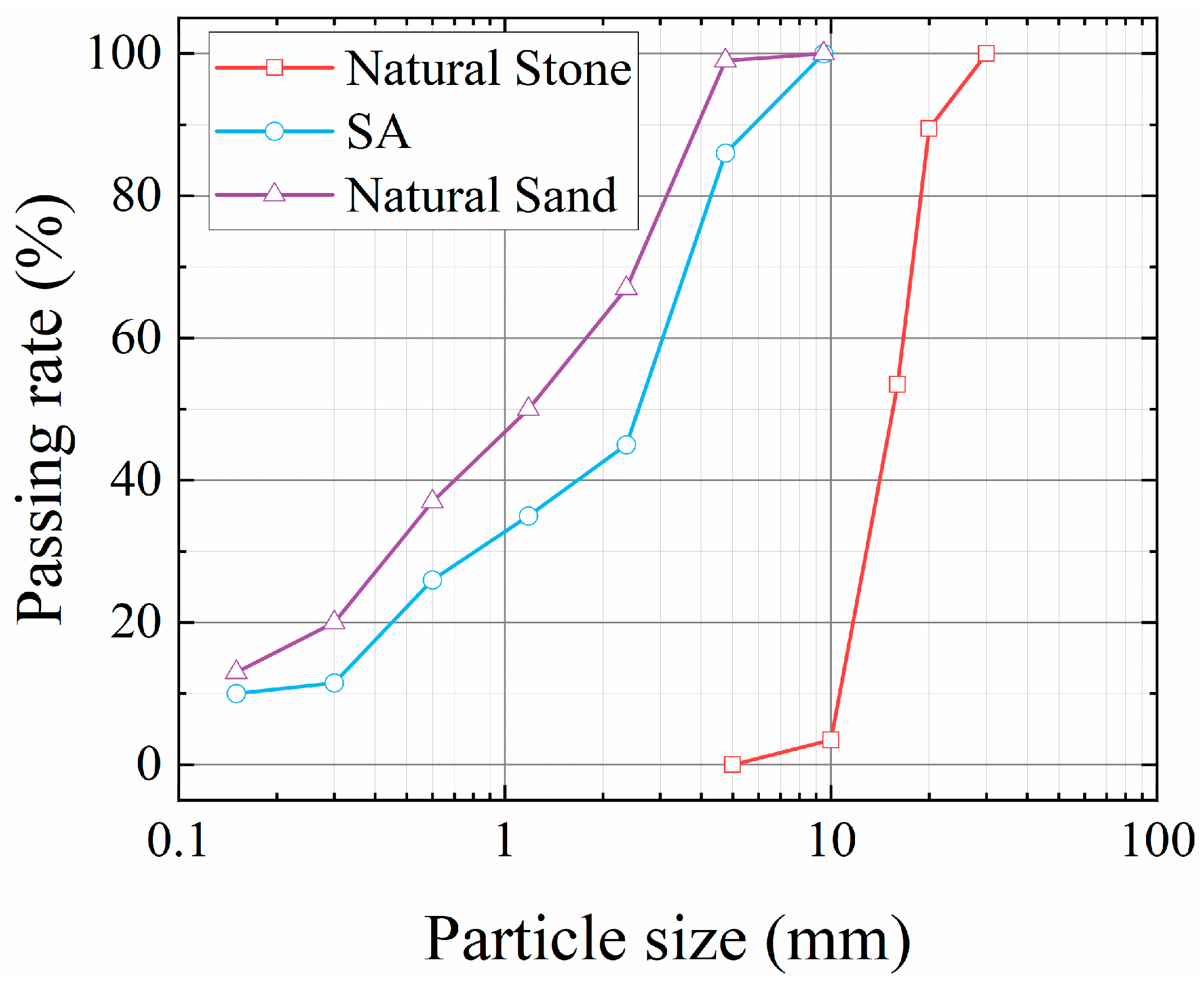
2.1. Raw Materials

The steel slag fine aggregate concrete (SC) used in the test was composed of P.O. 42.5 ordinary Portland cement (in accordance with the Chinese standard GB 175-2007 [36]), natural fine aggregate, steel slag fine aggregate (SA), natural coarse aggregate, water reducer, and water. The particle size distribution of the aggregates is shown in Figure 1. The main physical properties of SA and natural fine aggregate are presented in

Table 1. Physical properties of natural fine aggregate and SA.

Fine Aggregate	Apparent Density (kg/m3)	Loose Bulk Density (kg/m3)	Compact Bulk Density (kg/m3)	Crushing Value (%)	Silt Content (%)	Water Absorption (%)	Void Ratio (%)
Natural Sand	2677	1583	1653	15.96	2.81	0.84	41.0
SA	3261	1890	1950	9.59	3.66	2.87	40.6

.

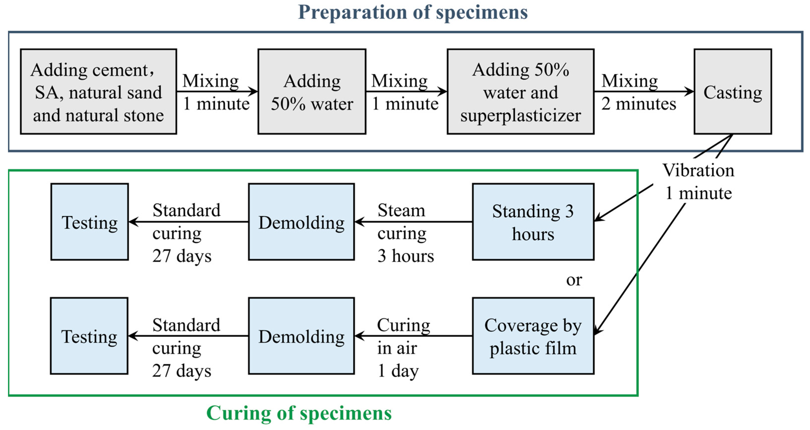
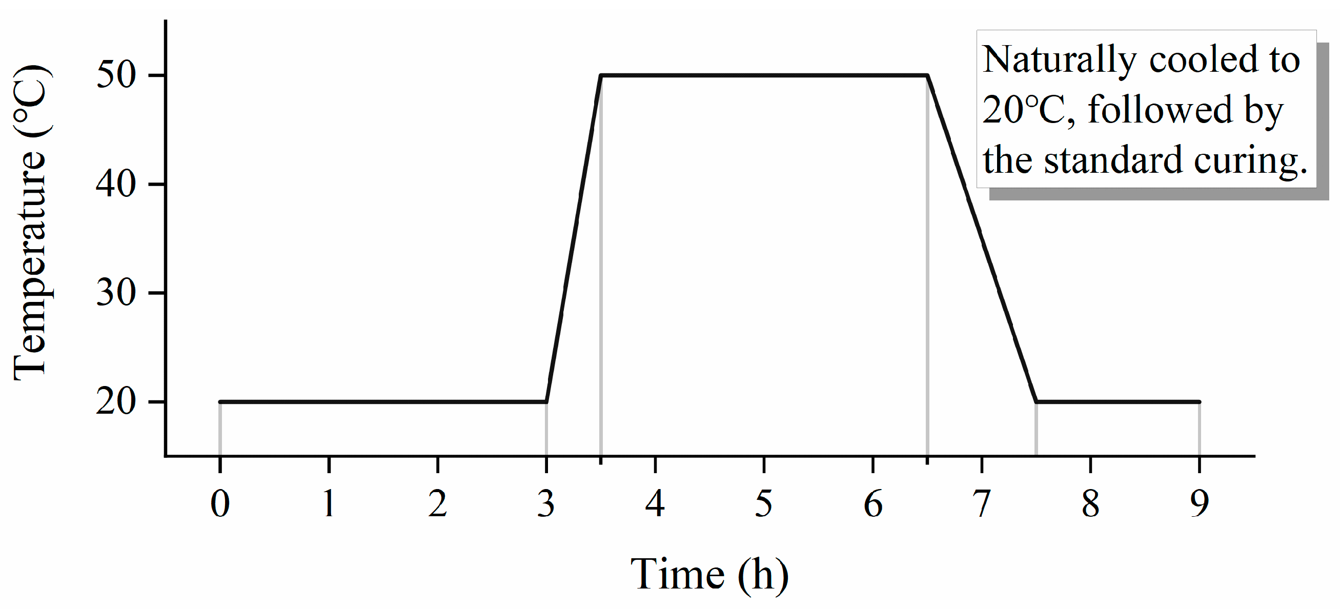
2.2. Specimen Fabrication and Mix Proportion

The concrete mix proportions, which include the naming and grouping of specimens according to different SA volume contents, different water–cement ratios, and different curing systems, are shown in

Table 2. Mix proportion of SC mixtures.

W/C	Series	Cement (kg/m3)	Fine Aggregate (m3/m3)	SA Replacement Rate by Volume	Natural Coarse Aggregate (kg/m3)	Water (kg/m3)	Water Reducer (kg/m3)
0.4	SC0.4-0~SC0.4-7, SC0.4-10	375.00	0.37	0%~70%, 100%	949.13	150.00	3.75~4.50
0.5	SC0.5-0~SC0.5-7, SC0.5-10	300.00	0.38		981.96		3.00~3.60
0.6	SC0.6-0~SC0.6-7, SC0.6-10	250.00	0.39		1003.52		2.50~3.00
0.5	SC0.5-0b~SC0.5-7b, SC0.5-10b	300.00	0.38		981.96		3.00~3.60

Note: w/c represents the water–cement ratio. SC_0.4-1 represents the steam-cured steel slag fine aggregate concrete specimen group with the 10% volume substitution rate of natural fine aggregate by SA, and with a water–cement ratio of 0.4. SC refers to steel slag fine aggregate concrete. _0.4 refers to the water–cement ratio, which could alternatively be _0.5 or _0.6. -1 specifies the 10% volume replacement rate of steel slag fine aggregate, which can be -0, -2, -3, -4, -5, -6, -7, and -10, corresponding to the volume replacement rate of 0%, 20%, 30%, 40%, 50%, 60%, 70%, and 100%, respectively. Similarly, SC_0.5-0b represents the standard-cured specimen group of steel slag fine aggregate concrete with a 0.5 water–binder ratio and 0% volume content. The steam-cured SC specimens were subjected to steam curing at 50 °C and 95% RH for 3 h, followed by standard curing at 20 °C and 95% RH for 28 days; the standard-cured SC specimens were cured at 20 °C and 95% RH for 28 days.

. In accordance with JGJ 55-2011 [37], SC was mixed using the SJD-100 forced single horizontal shaft concrete blender (Zhejiang Chenxin Machine Equipments Co., Ltd., Shangyu, China). The preparation and curing process of SC specimens is illustrated in Figure 2. The steam curing was carried out using the NBSCH fully automatic electric heating steam generator (Wuhan Nobeth Machinery Manufacturing Co., Ltd., Wuhan, China), and the temperature variation curve of SC steam curing is shown in Figure 3. After the specimens were cast, they were kept at an ambient temperature (25 °C) for 3 h prior to being transferred to the steam curing environment. The temperature was increased to 50 °C within 0.5 h, and then the specimens were steam-cured at 50 °C for 3 h. After natural cooling to room temperature, the specimens were transferred to the standard curing environment that conforms to GB/T 50081-2019 [38] for further curing until the designated time.

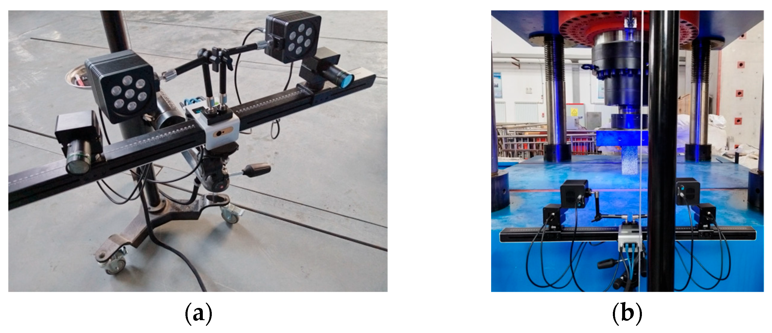
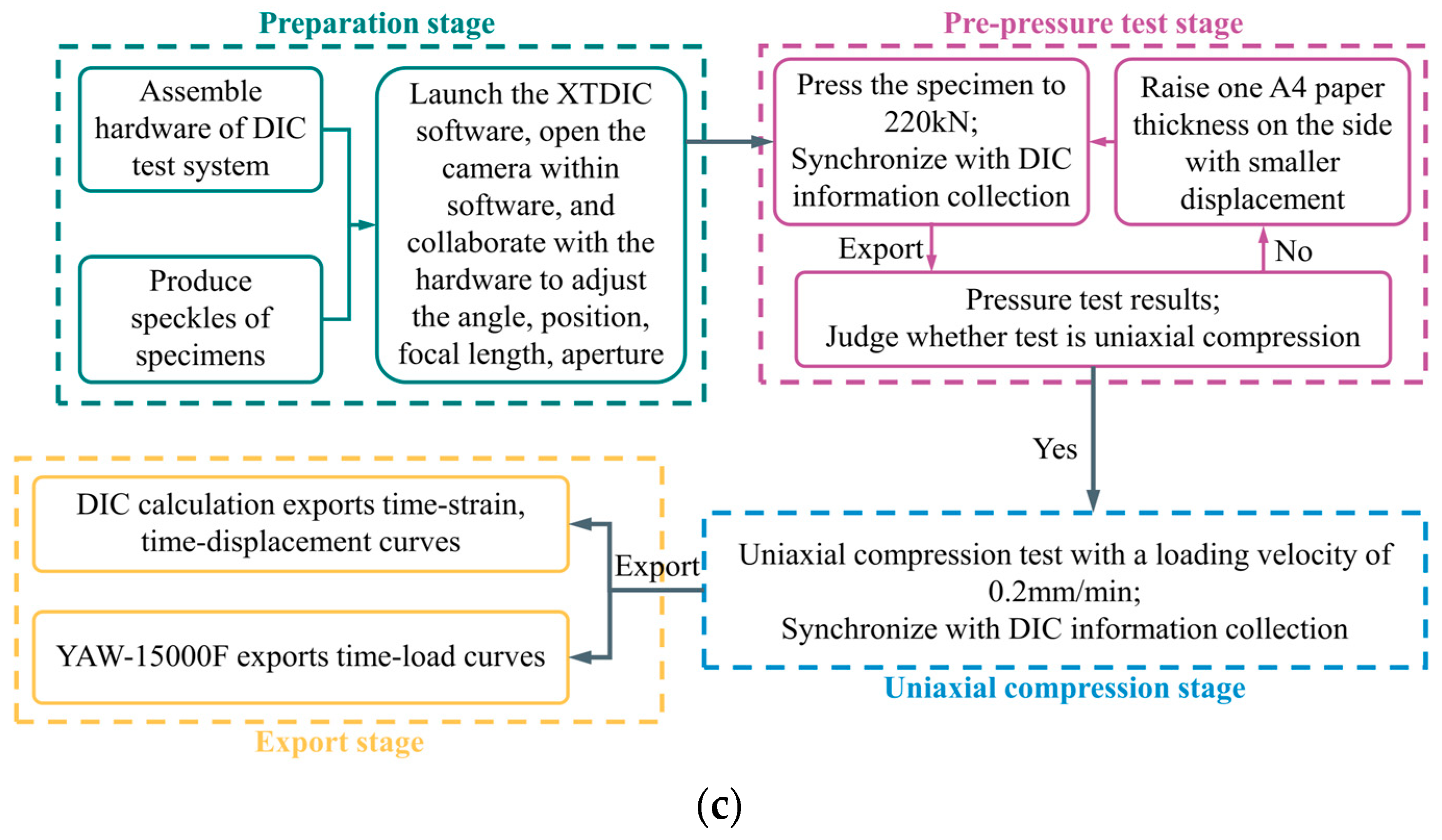
2.3. Uniaxial Compression Test Method

The stress–strain test of SC under uniaxial compression was performed using the YAW-15000F electro-hydraulic servo multifunctional structural test system (Popwil Instrument Co., Ltd., Hangzhou, China) and the XTDIC-3D non-contact full-field strain measurement system (XTOP 3D Technology Co., Ltd., Shenzhen, China), as seen in Figure 4a,b. To reduce the occurrence of pseudo-strain [39,40], the loading rate of 0.2 mm/min was maintained throughout the uniaxial compression test. The detailed procedure for the uniaxial compressive stress–strain test is shown in Figure 4c. Following the preparation of the specimen and the setup of the hardware, the pre-pressure test was conducted. According to the GB/T 50081-2019 [38], the specimen was compressed at the rate of 0.6 mm/min until a load of 220 kN was reached. Similar to the strain data collection methods employed by Zhou et al. [41] and Wang et al. [42], Digital Image Correlation (DIC) was utilized to concurrently gather strain data from the specimen. The DIC output results were analyzed to verify whether the test was uniaxial compression [43]. If the displacement variation on both sides at the same height remained within 0.078 mm, the test was deemed to be uniaxial compression, and the formal uniaxial compressive stress–strain test could proceed. Conversely, if the variation exceeded this threshold, the side with less displacement was elevated by the thickness of a piece of A4 paper, and the pre-pressure test was repeated to reassess uniaxial compression. This adjustment and retesting process was iterated 2 to 3 times until the specimen was confirmed to be under uniaxial compression. It is worth noting that the acquisition frequency for stress and strain data should be consistent for each specimen in both systems.

Three prismatic SC specimens, each measuring 150 mm × 150 mm × 300 mm, were prepared. During the uniaxial compression process, the initial failure regions might only indicate cracking or spalling, rather than representing the failure at the specimen’s ultimate strain [44]. To accurately represent the entire stress–strain process, the stress–strain curve should be plotted using the later failure points from the central region (center point, ±75 mm vertically, ±37 mm horizontally) of the specimen.

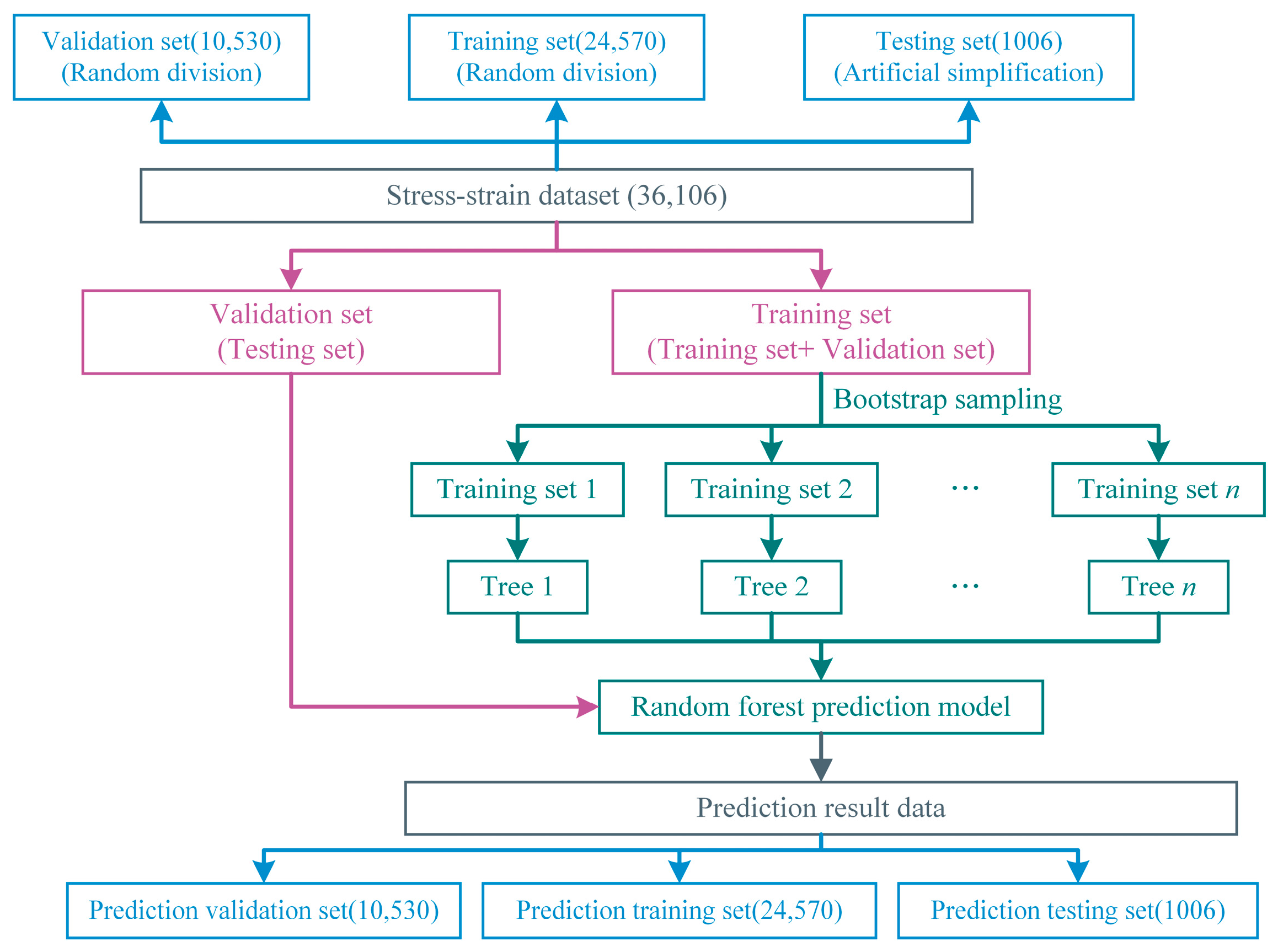
2.4. Random Forest (RF) Prediction Model

The uniaxial compressive stress–strain dataset obtained from the test contains 36,106 data points. It was artificially thinned to obtain 1006 data points as the testing set, which is the same as the data points used for plotting the stress–strain curves. This facilitates the further comparison of the predicted curves from the testing set with the actual test curves to assess accuracy. The remaining 35,100 data points were randomly divided into 3:7 ratios, resulting in a validation set composed of 10,530 data points and a training set consisting of 24,570 data points. In addition to the RF algorithm, the backpropagation neural network algorithm and support vector regression algorithm also adopted the same dataset division method.

The random forest algorithm is particularly effective for large datasets. Even with hundreds or thousands of input variables, it does not overfit and does not require data pruning. Moreover, the algorithm is highly efficient in selecting feature subsets and imputing missing data [45]. In the RF prediction model, the number of trees was set to 100; the minimum number of samples required to split a node was set to 2; the minimum sum of weights for leaf nodes was set to 1; and the maximum depth of a single decision tree was set to zero, allowing the trees to grow as much as possible until each leaf node is pure. The random seed was set to 42 to control randomness. Figure 5 illustrates the structure of the RF prediction model. The model operation process is carried out in two stages: First, using Bootstrap sampling, 70% of the 35,100 data points, which is 24,570 data points, were randomly selected as the training set to construct n training subsets, and then n decision trees were generated corresponding to these n training subsets. For each branch node of each decision tree, k feature variables were first randomly selected from the m feature variables, and then the optimal feature parameter was chosen from the selected k feature variables for dividing. This process was repeated multiple times to form the random forest prediction model. The parameter k controls the degree of randomness introduced, and the recommended value is k = log₂m. Second, the model was trained using the 35,100 data points from both the training and validation sets, and the new RF model was obtained by running the aforementioned steps. The model was then tested using the 1006 data points from the testing set.

2.5. Backpropagation Neural Network (BPNN) Prediction Model

The BPNN is a learning principle of the feedforward network, which uses the gradient descent method to readjust the network connection weights to minimize the RMSE between the predicted output and the test result [24]. Too many hidden layers may lead to overfitting, while the BPNN with a single hidden layer can simulate complex nonlinear relationships well after training [24]. During the trial run phase of the BPNN, the performance of the BPNN on the validation set was monitored, and training was halted when the performance on the validation set began to decline, indicating that the BPNN had started to overfit. The overfitting issue of the BPNN was addressed by reducing the number of hidden layers and controlling the number of neurons in each layer to decrease network complexity. Through multiple comparisons of the prediction results and statistical evaluation metrics of BPNN with different numbers of hidden layers and different numbers of neurons in the hidden layers during the trial run phase, the appropriate BPNN structure was ultimately determined. Therefore, the network structure adopts a single hidden layer with 64 neurons. The water–cement ratio (a₁), volume content of SA (a₂), and strain (a₃) serve as the three input neurons. The Levenberg–Marquardt algorithm [46,47] is employed for model training. Figure 6 illustrates the BPNN prediction model structure diagram. w_1,1 represents the connection weight between the input layer variable a₁ and the hidden layer neuron b₁. v_1,1 represents the connection weight between the hidden layer neuron b₁ and the output layer c₁. The training set data are input into the network from the input layer. At the start of training, the signals from the input layer are transmitted to the hidden layer, and after processing, the actual output signals are obtained at the output layer. The error between the test data and the predicted output is calculated. If the error is within the allowable range, the training is terminated. Otherwise, the error signal is backpropagated. The error is backpropagated through the gradient descent method [48] to train the weights and thresholds of each layer of the neural network, thereby continuously reducing the error. The above steps are repeated until the error reaches the allowable error or the number of iterations reaches the preset maximum.

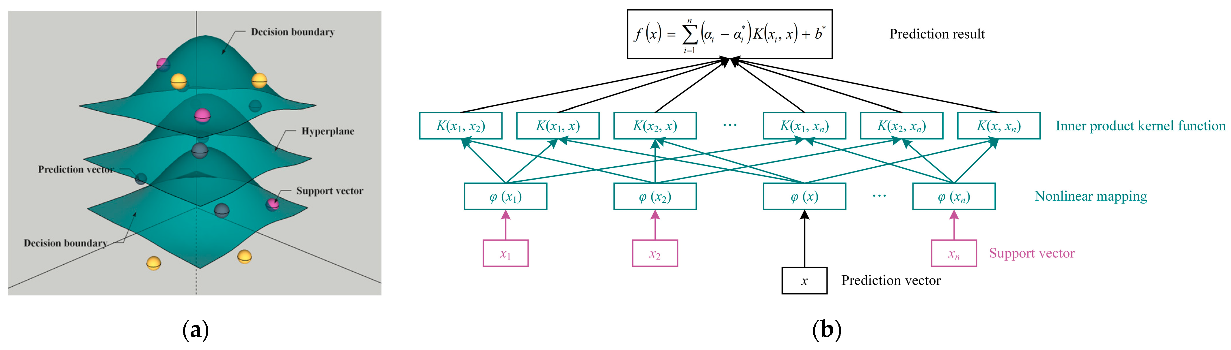
2.6. Support Vector Regression (SVR) Prediction Model

The principle of SVR [49] is to map the feature vectors of samples to the high-dimensional space and find a hyperplane in the feature space that minimizes the “distance” to the farthest sample point. The principle of the SVR prediction model is shown in Figure 7a. During the trial run phase of the SVR, the regularization parameter was adjusted, and the appropriate kernel function was selected. The prediction performance of the SVR was continuously compared after each trial run to avoid model overfitting and to obtain the suitable SVR model. In this paper, the SVR prediction model uses the Gaussian Radial Basis Function Kernel (RBF) as the kernel function, and Figure 7b shows the structural diagram of the SVR prediction model. First, the data are normalized, and then the model is trained and used for prediction. The support vectors and the vectors to be predicted in the low-dimensional space are nonlinearly mapped to a high-dimensional space where they are linearly separable. Then, the inner product kernel function calculation is performed between the prediction vectors and the support vectors to avoid a large number of inner product calculations. Regression is then carried out to obtain the output regression data. The data results are inversely normalized, and the final prediction results are output.

3. Results and Discussion

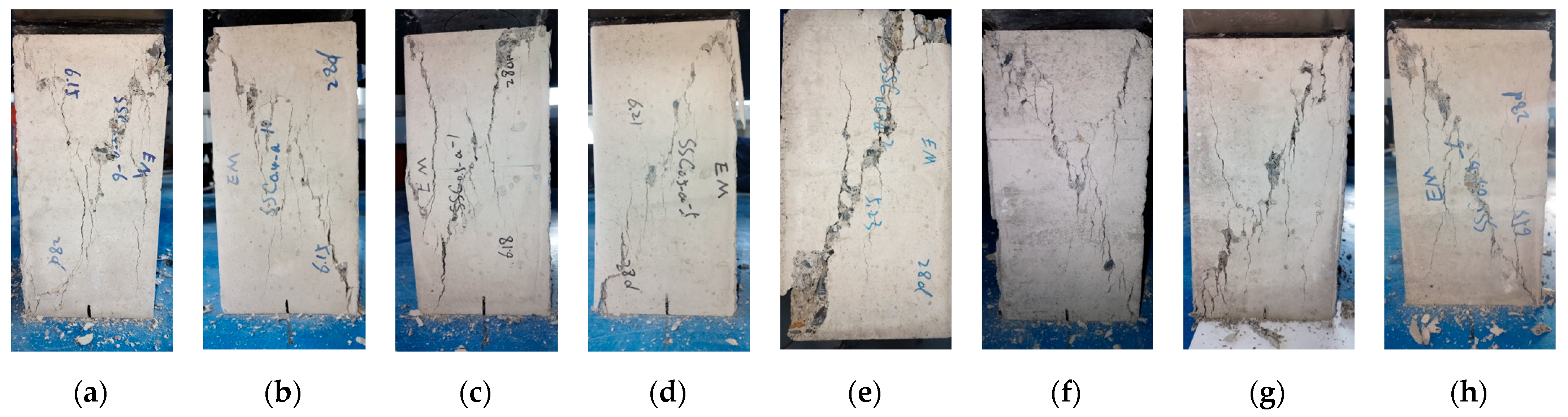
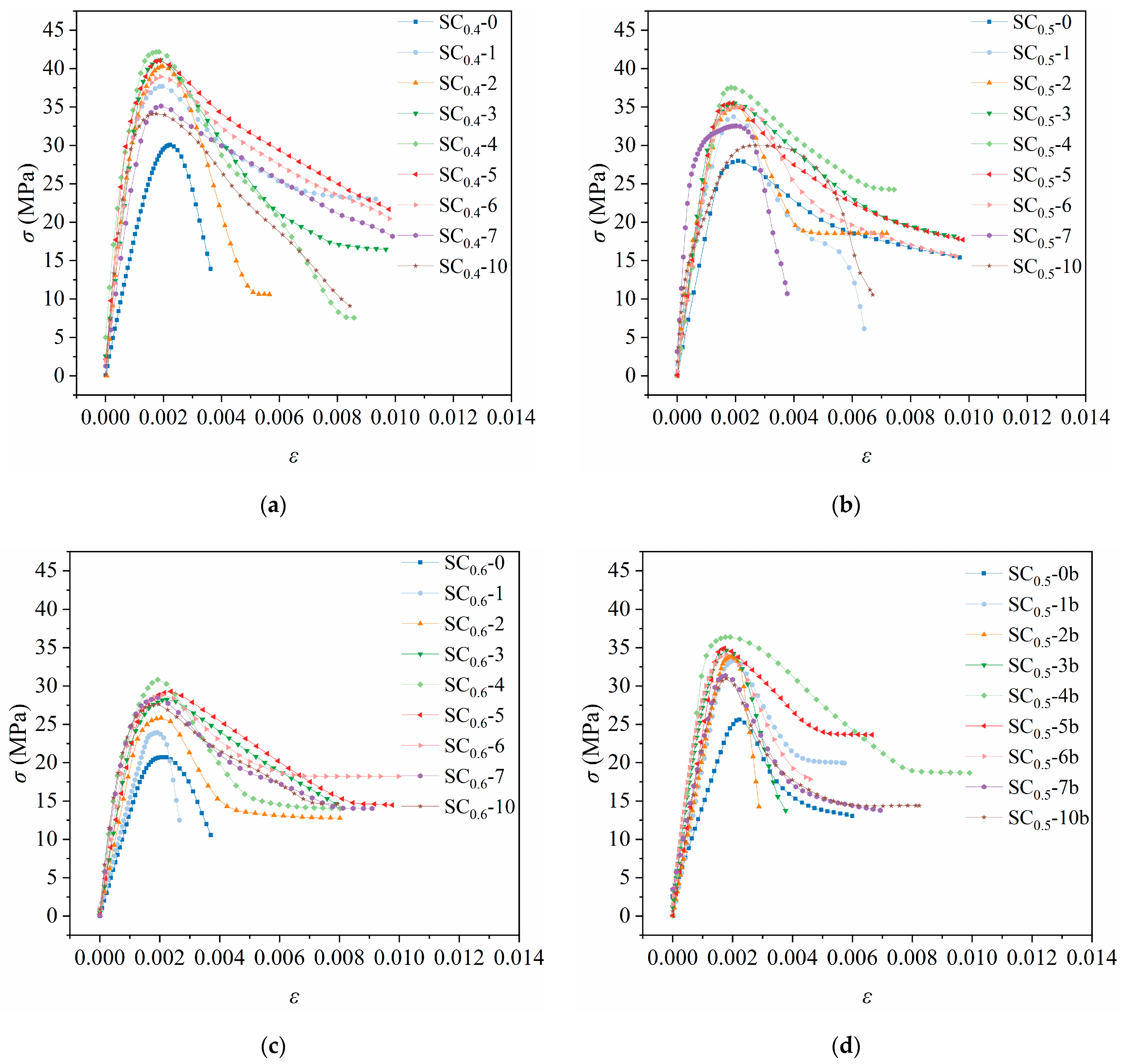
3.1. Uniaxial Compression Failure and Stress–Strain Curves

The SC specimens all exhibited uniaxial compression failure, with the side surfaces of the specimens being the main fracture surfaces. Through the uniaxial compression tests on the SC specimens, it was found that the main cracks developed parallel to the loading direction and eventually formed penetrating cracks along the diagonal. The main fracture surfaces of some SC specimens under uniaxial compression failure are shown in Figure 8. Cracking, crack propagation, and specimen failure are the three stages of the failure process of SC specimens. During the plastic deformation stage of the uniaxial compression test, internal microcracks begin to form. As the internal cracks gradually increase in number, surface cracks start to appear and multiply rapidly when the peak stress is reached. With the extension and widening of the cracks, the cracks penetrate the specimen, leading to the failure of the specimen.

The 28-day uniaxial compressive stress–strain (σ–ε) relationship of SC specimens are shown in Figure 9. As seen in Figure 9a–c, when the SA volume content is 40%, the steam-cured SC specimens have a higher peak stress. The ultimate strain of the steam-cured SC specimens is synthetically greater than that of the standard-cured SC specimens. Moreover, the descending branch of the steam-cured SC is generally more gentle than that of the standard-cured SC, indicating that the ductility of the SC specimens is improved by steam curing. The main reason for the above results is that steam curing accelerated the hydration of SA in the SC specimens, which in turn produces more hydration products that filled the microvoids in the concrete, thereby improving the density of the concrete [44].

3.2. Stress–Strain Prediction Models Based on RF, BPNN, and SVR

The 28-day stress prediction results of steam-cured SC based on RF, BPNN, and SVR models are presented in Figure 10, Figure 11 and Figure 12, respectively. Compared with the BPNN and SVR models, the RF model performs better in predicting the stress of steam-cured SC. The prediction results of the training and validation sets show that the RF model can accurately predict stress values, with almost all points falling within the error band of ±15% from the test results (y = x), although there are a few individual data points with deviations when the stress is in lower states. The prediction performance of the BPNN model for the training and validation sets is not as good as that of the RF model, with some points exceeding the ±15% error band of the test results, but it is better than the SVR prediction model. The prediction characteristic of the SVR model is that it shows coherent prediction points. This is because SVR achieves the regression prediction of data by finding a hyperplane in the feature space, thereby being able to handle high-dimensional data and nonlinear problems. However, many points of the SVR model exceed the ±15% error band of the test results, and the distribution of points is relatively discrete, indicating significant deviations exist between the predicted and actual values. Figure 10, Figure 11 and Figure 12 show that the SVR model performs worse than the RF and BPNN models, with a poorer generalization ability.

As shown in Figure 10c, Figure 11c and Figure 12c, the prediction deviations of the testing sets for the three models once again confirm the aforementioned conclusions. For the RF and BPNN models, most prediction errors are basically stable at a stress = 0, while many prediction errors of the SVR model fluctuate above and below the 0 horizontal line.

The judgment of whether a machine learning model is overfitted mainly relies on the following two aspects: on the one hand, compare the errors of the training set and the validation set. If the error of the model on the training set is very small, but the error on the validation set or the test set is very high, it indicates that the model may be overfitted. Ideally, the errors of the training set and the validation set should be close. On the other hand, the judgment is based on the scatter plot of the true values and the predicted values. If the scatter points are closely distributed around the straight line y = x, this indicates that the prediction effect of the model is good; if the scatter points are randomly distributed or deviate far from the straight line, it may be overfitted. The scatter plots of the three models do not show serious clustering or dispersion, indicating that the prediction models do not exhibit obvious underfitting or overfitting.

3.3. Evaluation of the Accuracy of RF, BPNN, and SVR Prediction Models

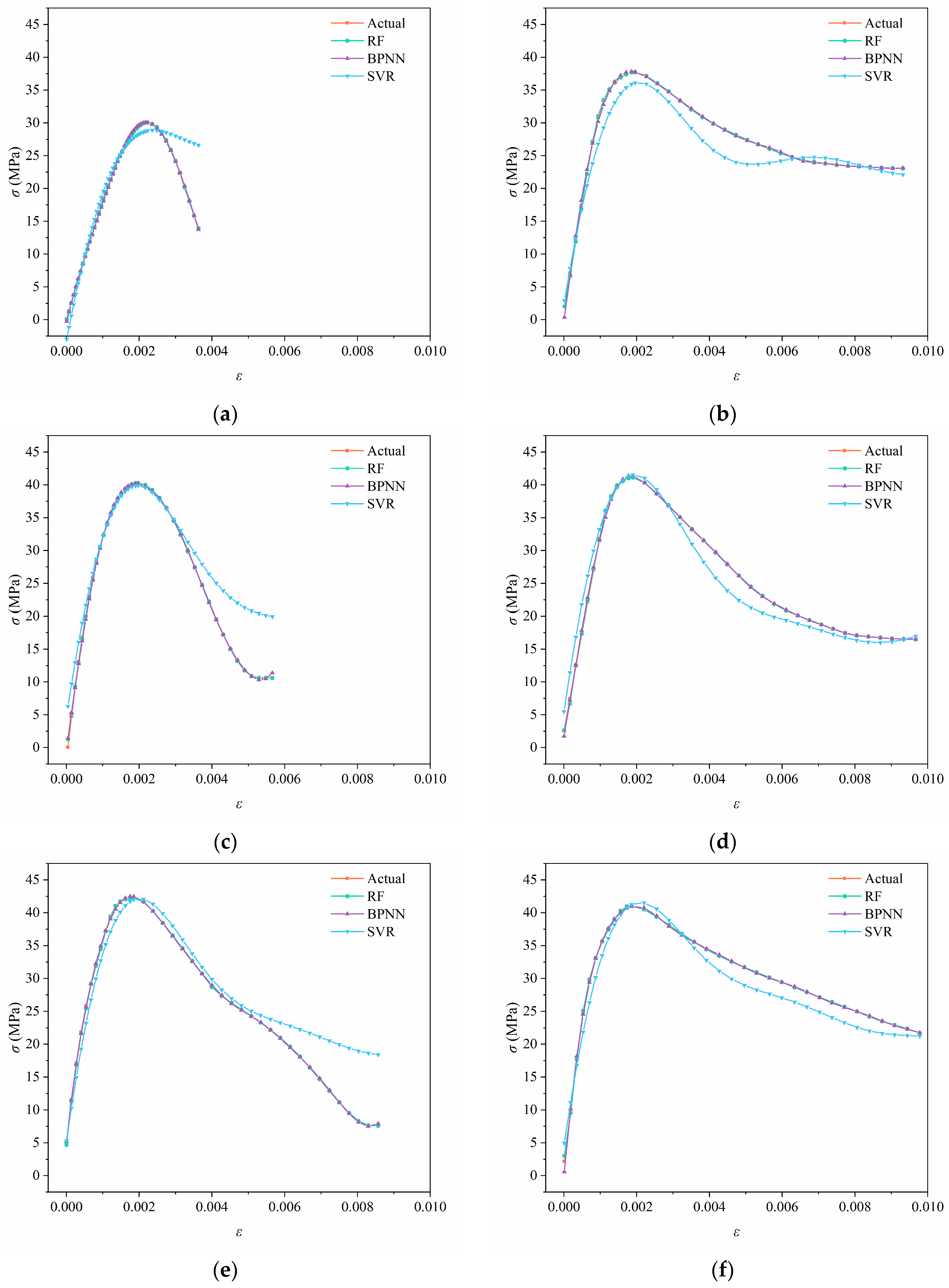
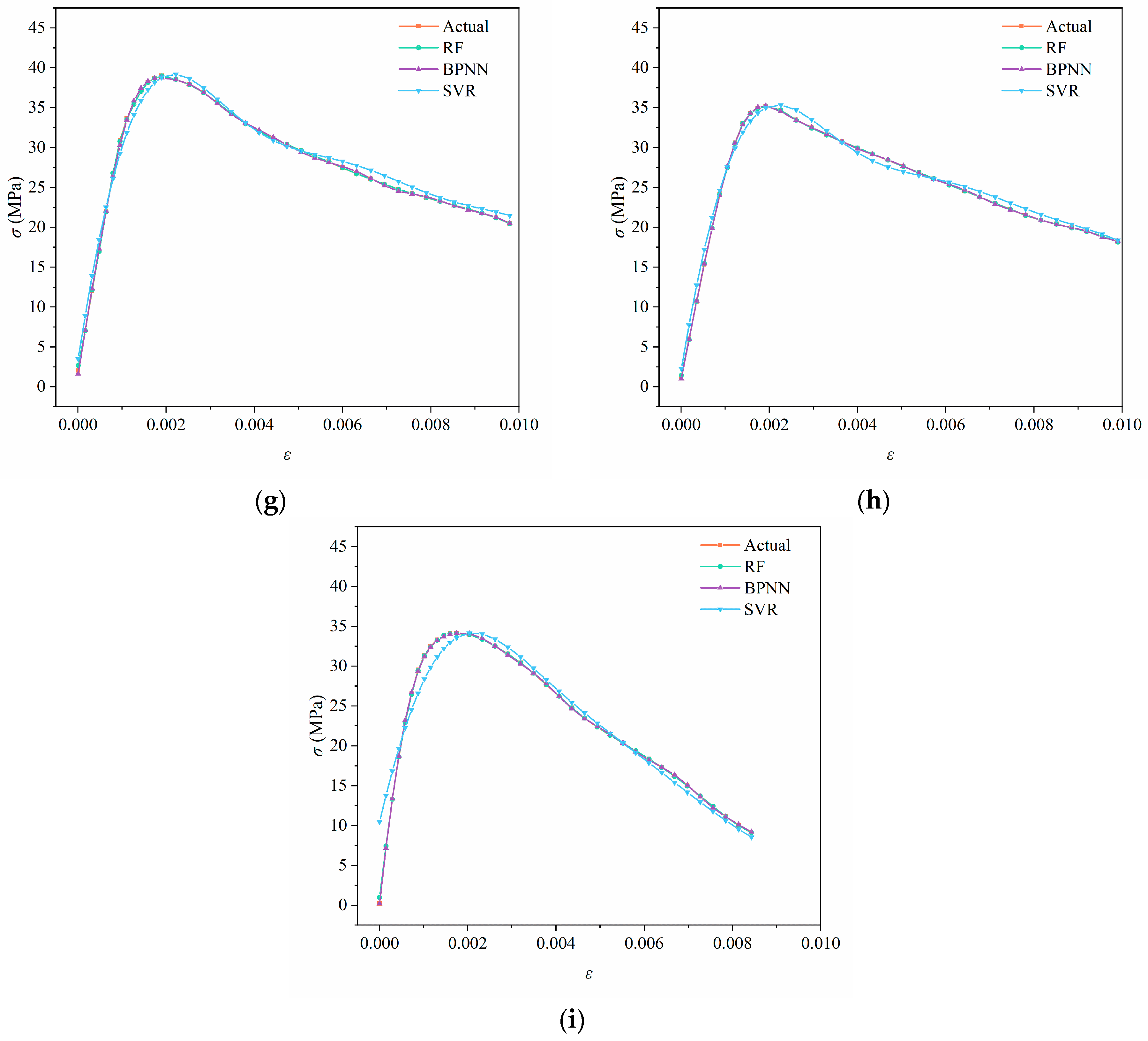
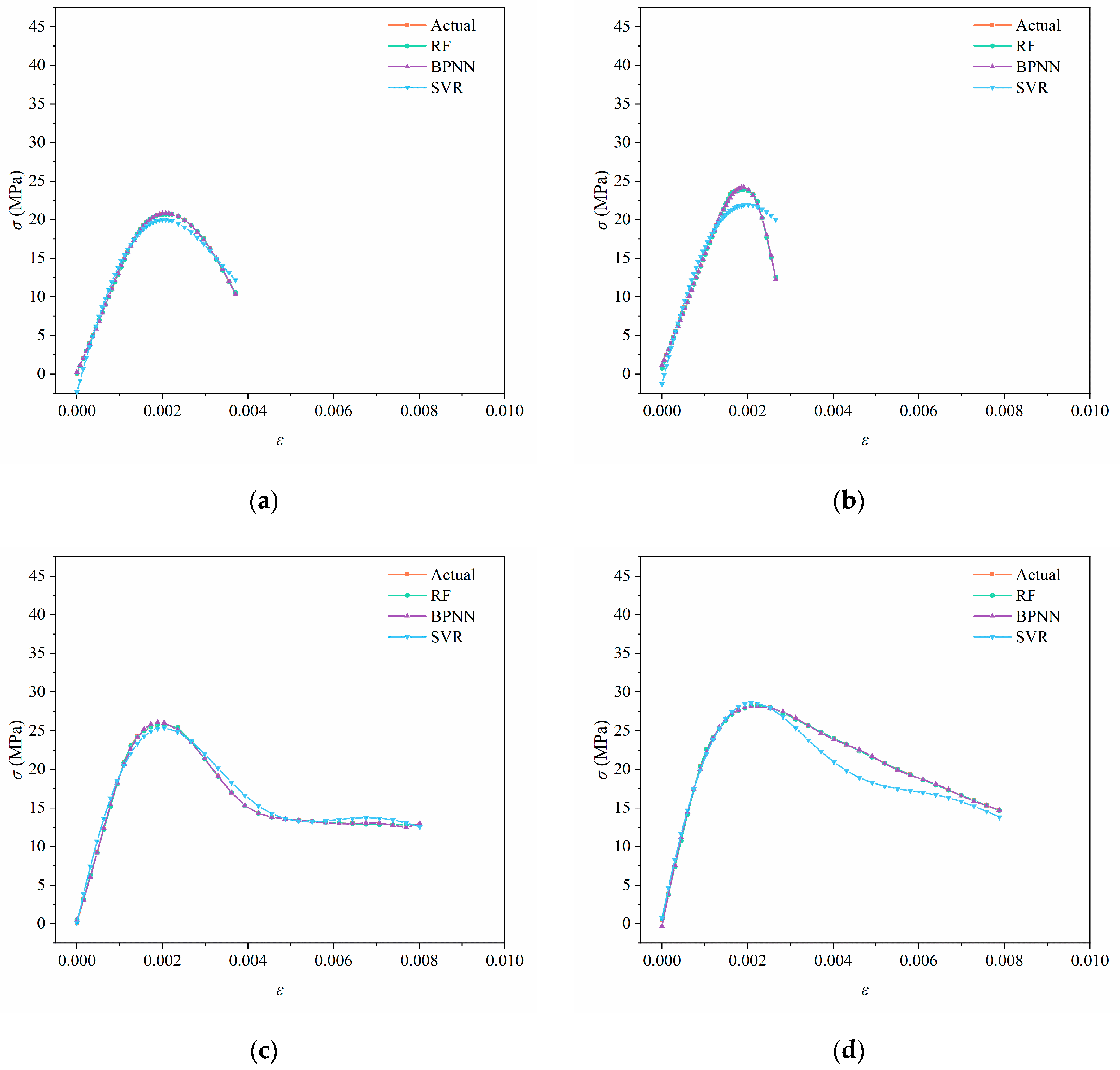
3.3.1. Prediction Results of the Testing Set

Figure 13, Figure 14 and Figure 15 show the stress prediction results of the testing sets for steam-cured SC with water–cement ratios of 0.4, 0.5, and 0.6 by the three models, respectively. The RF and BPNN models predict the actual data more accurately, while the SVR model has larger errors. The deviation of the SVR model increases dramatically in the descending branch. Overall, in terms of prediction performance, RF > BPNN > SVR. The RF model can generally predict stress values accurately, but there are still a few rare cases where RF makes incorrect predictions. For instance, in Figure 14e, the prediction of the ultimate stress of SC_0.5-4 by RF, which is at the end of the descending branch, deviates from the actual value. In this case, the prediction performance of RF is even worse than that of BPNN and SVR. The above situation is not unique to the RF model. BPNN-predicted values always closely match the actual stress values in the descending branch but occasionally deviate in predicting the ultimate stress, as seen in Figure 13c, Figure 14a,i and Figure 15g. Although the SVR model has the worst prediction performance, it has some instances where its predicted values closely match the actual stress values, such as in Figure 13g,h and Figure 14a,c–e,g,i. Considering all factors, the prediction performance of the SVR model on the testing set is not as good as that of the RF and BPNN models. The RF and BPNN models show great potential for predicting the stress of steam-cured SC using the water–cement ratio, SA volume replacement rate, and SC strain as input variables.

3.3.2. Model Prediction Accuracy

Three statistical evaluation metrics, R², MAE, and RMSE [24,32,50], are used to assess the prediction accuracy of the models, as shown below:

$${\mathit{R}}^2=1-{\displaystyle \frac{{\sum }_{\mathit{i}=1}^{\mathit{m}}{\left({\mathit{y}}_{\mathit{i}}-{\widehat{\mathit{y}}}_{\mathit{i}}\right)}^2}{{\sum }_{\mathit{i}=1}^{\mathit{m}}{\left({\mathit{y}}_{\mathit{i}}-\stackrel{\mathrm{-}}{\mathit{y}}\right)}^2}}$$

(1)

$$\mathit{MAE}={\displaystyle \frac{1}{\mathit{m}}}\sum _{\mathit{i}=1}^{\mathit{m}}\left|{\mathit{y}}_{\mathit{i}}-{\widehat{\mathit{y}}}_{\mathit{i}}\right|$$

(2)

$$\mathit{RMSE}=\sqrt{{\displaystyle \frac{1}{\mathit{m}}}\sum _{\mathit{i}=1}^{\mathit{m}}{\left({\mathit{y}}_{\mathit{i}}-{\widehat{\mathit{y}}}_{\mathit{i}}\right)}^2}$$

(3)

where m is the number of data samples; y_i is the true stress (σ) test value of the sample; ${\widehat{\mathit{y}}}_{\mathit{i}}$ represents the predicted stress (σ) value of the sample; and $\stackrel{\mathrm{-}}{\mathit{y}}$ is the average of the true stress (σ) values of the data sample.

The R² value quantitively describes the accuracy of the predictive model. The closer the R² value is to 1, the better the prediction performance. The MAE and RMSE are defined as parameters for evaluating prediction performance based on the accumulation of errors [32]. Therefore, only smaller MAE and RMSE values can indicate that the model has better prediction performance.

The statistical evaluation metrics for each model’s predictions on different data subsets are shown in

Table 3. Statistical evaluation metrics of the models.

Prediction Models and Data Subsets		R2	MAE	RMSE
RF	Training set	1.0000	0.0185	0.0450
	Validation set	1.0000	0.0464	0.1497
	Testing set	1.0000	0.0473	0.1282
BPNN	Training set	0.9993	0.1403	0.2176
	Validation set	0.9994	0.1416	0.2203
	Testing set	0.9990	0.1831	0.2896
SVR	Training set	0.9214	1.4820	2.3493
	Validation set	0.9221	1.4658	2.3271
	Testing set	0.9432	1.3955	2.2109

. In terms of the vertical comparison, the RF model shows extraordinary performance compared to BPNN and SVR, with an R² = 1.00 for the testing set, validation set, and training set. Compared with studies [51,52,53,54,55] using machine learning models for predicting the concrete compressive strength, the RF model’s performance in predicting the stress of steam-cured SC is amazing. Additionally, the R² of the BPNN model can also reach 0.99, allowing it to accurately predict the stress of steam-cured SC. However, the BPNN model has higher MAE and RMSE than the RF model, indicating that its prediction error is greater than that of the RF model. Among the three models, the SVR model still has the worst prediction performance, with an R² value lower than the other two and higher MAE and RMSE values than the other models. In terms of a horizontal comparison, the prediction accuracy of the RF and BPNN models decreases as the amount of data in the data subset decreases. However, the SVR model is the opposite, with better prediction performance on the testing set than on the training and validation sets. Whether the SVR model has advantages for small datasets still needs further testing and verification.

4. Applicability of the Models

4.1. Reconstruction of RF and BPNN Models

As shown in Section 3, both RF and BPNN models exhibit good predictive performance for the stress–strain relationship of steam-cured SC under random data divisions or artificial data thinning. However, such data partitioning methods and algorithm operation mechanisms deviate from the actual engineering needs to some extent. In practical engineering applications, it is usually necessary to establish the prediction model based on the uniaxial compression performance of specimens with known mix proportions, and then infer the mechanical behavior of specimens with unknown mix proportions, providing theoretical support for concrete component design and structural reliability analysis.

Based on the existing stress–strain data of concrete mix proportion specimens, a constitutive model is fitted to predict the stress–strain curves of specimens with unknown mix proportions [56]. The gap between the predicted and measured curves is compared to assess the practical value of the model in engineering applications. This validation method is analogous to the concept of transfer learning. Transfer learning is a machine learning technique that enables the application of knowledge acquired from one task to another related task. By leveraging the features or parameters of pre-trained models, it significantly enhances the performance of the target task, especially when data are limited. This method has several notable characteristics: First, it effectively reduces training time and computational resources, as pre-trained models have already learned general feature representations. Second, transfer learning can substantially improve the generalization ability of models, enabling better performance on new tasks. Additionally, it can mitigate the issue of limited data in the target task by fine-tuning pre-trained models to adapt to new data distributions. The main advantages of transfer learning lie in its efficiency and flexibility.

Fu [12] and Xue [44] focused on analyzing the impact of the steel slag aggregate content on the stress–strain model of concrete. Zheng [35] discussed the relative importance of input variables in stress–strain prediction models based on machine learning for recycled aggregate concrete, and the results showed that compared with other input variables, the recycled aggregate replacement rate exhibited a higher importance. Therefore, the evaluation of the steam-cured concrete stress–strain prediction performance of RF and BPNN models when the volume replacement ratio of SA changes should be carried out. To evaluate the generalization ability of the models in predicting SC stress across different SA volume replacement ratios, the transfer learning validation method was used: the stress–strain data of steam-cured SC specimens with three water–cement ratios and SA replacement ratios of 30%, 50%, and 70% (12,088 data points) were used as the testing set, while the remaining 24,018 data points from specimens with other SA volume replacement ratios were used as the training set. The stress–strain dataset of steam-cured SC under uniaxial compression obtained from the tests is still being utilized. By training the RF and BPNN models and using the models to predict the stress values of specimens with SA replacement ratios of 30%, 50%, and 70% (not included in the training set) as the strain develops, the applicability of the models to the stress–strain relationship of SC with untrained mix proportions can be systematically tested.

In the initial operation phase of the BPNN prediction model, it was found that the prediction performance of the BPNN model with the original model parameters (64 hidden layer neurons) was not satisfactory. After parameter optimization and adjustment, when the number of hidden layer neurons was reduced to eight, the overfitting problem was alleviated by simplifying the network structure, and the BPNN model showed better prediction performance. The RF model in this section still uses the original parameters.

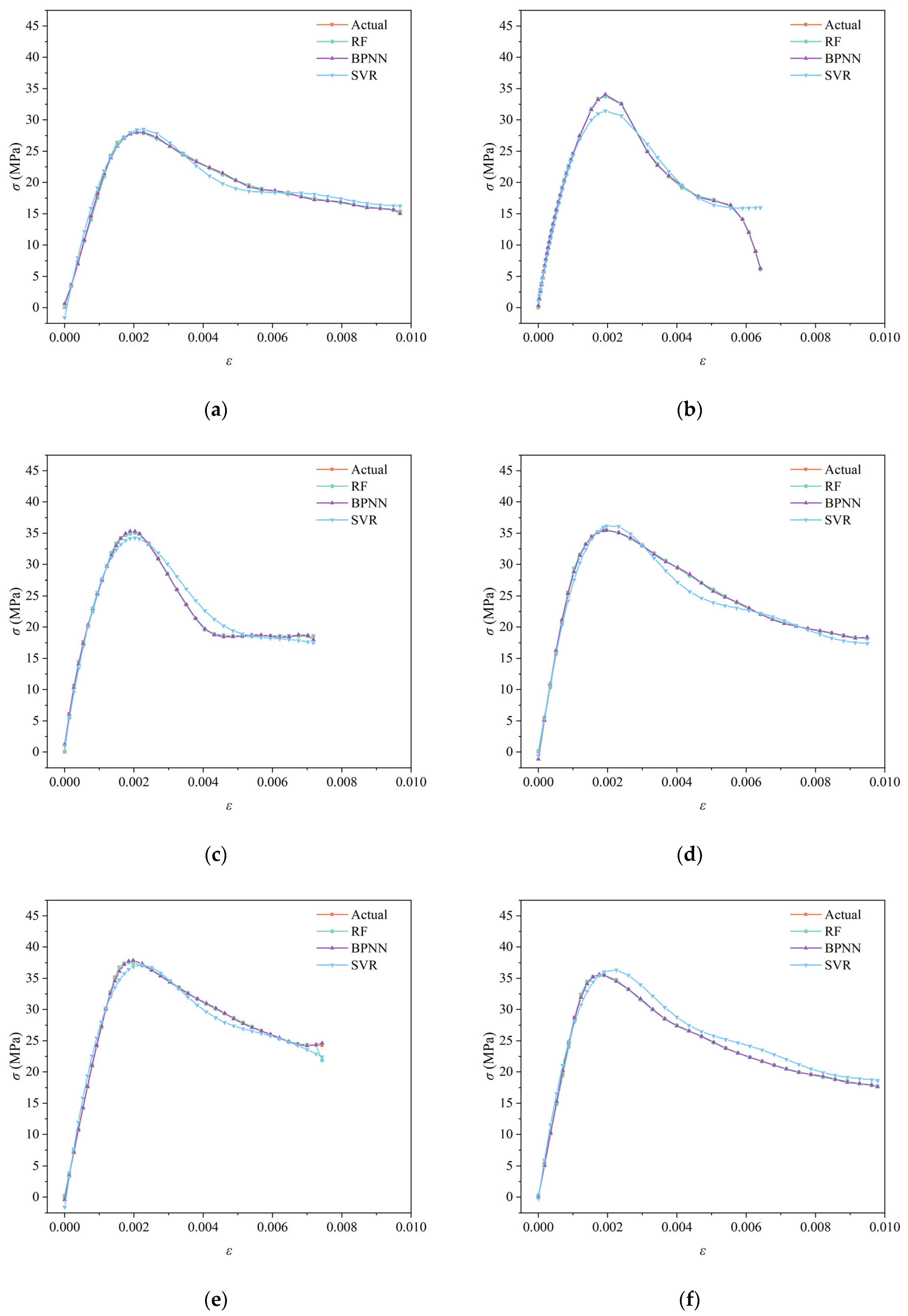
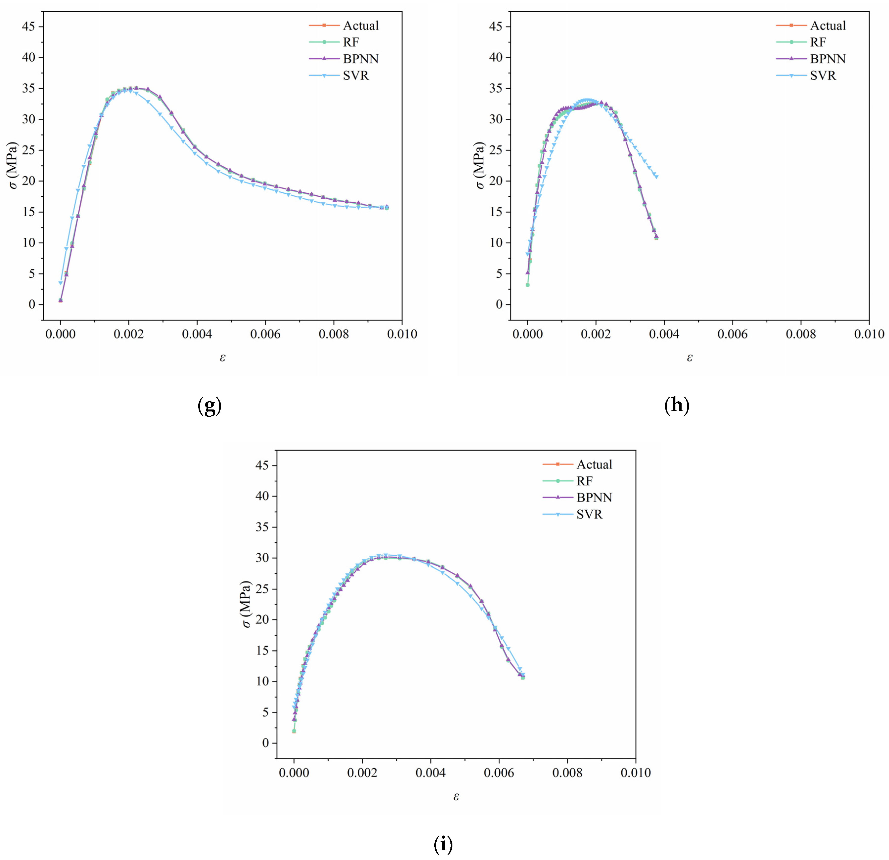
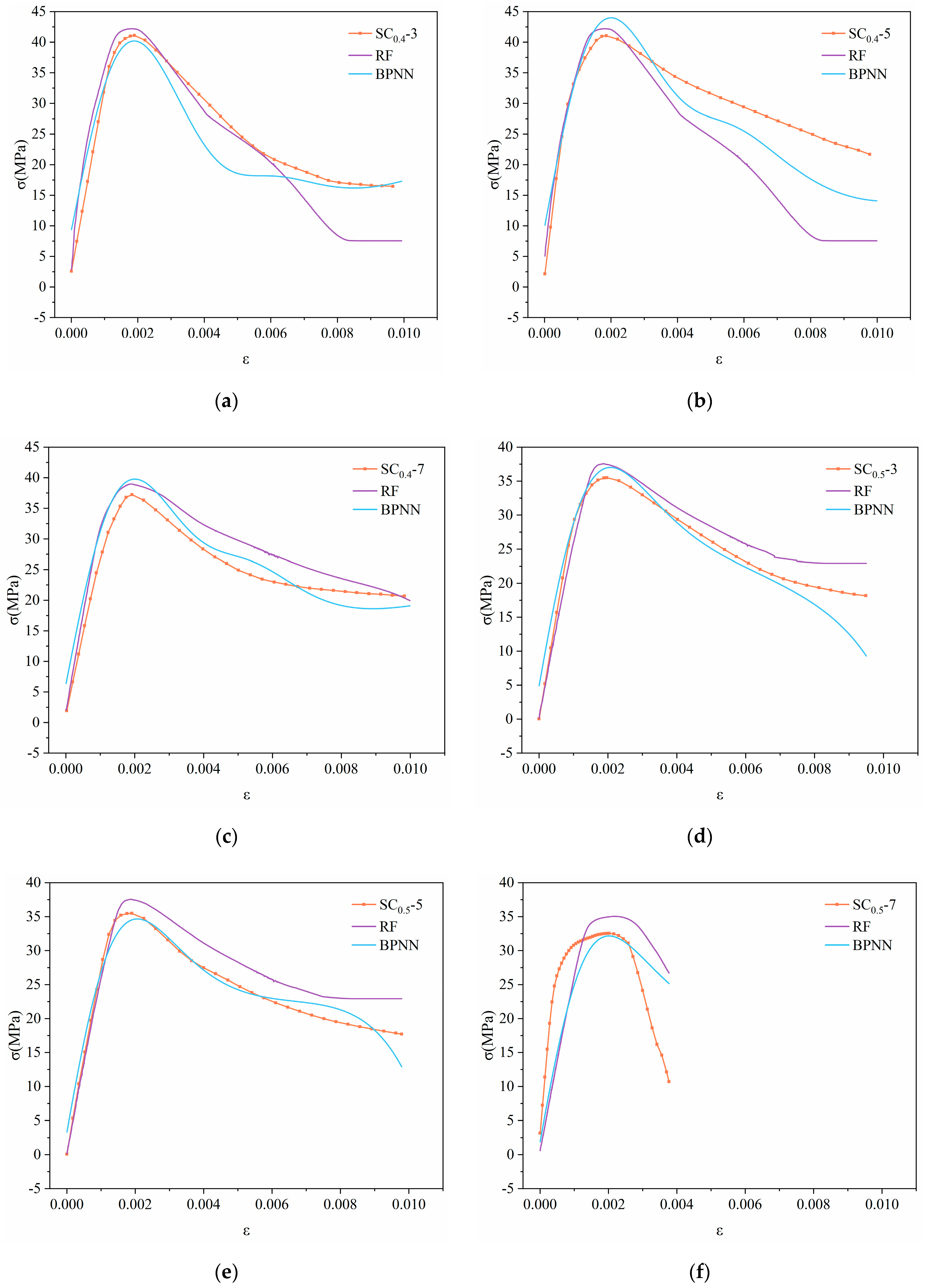
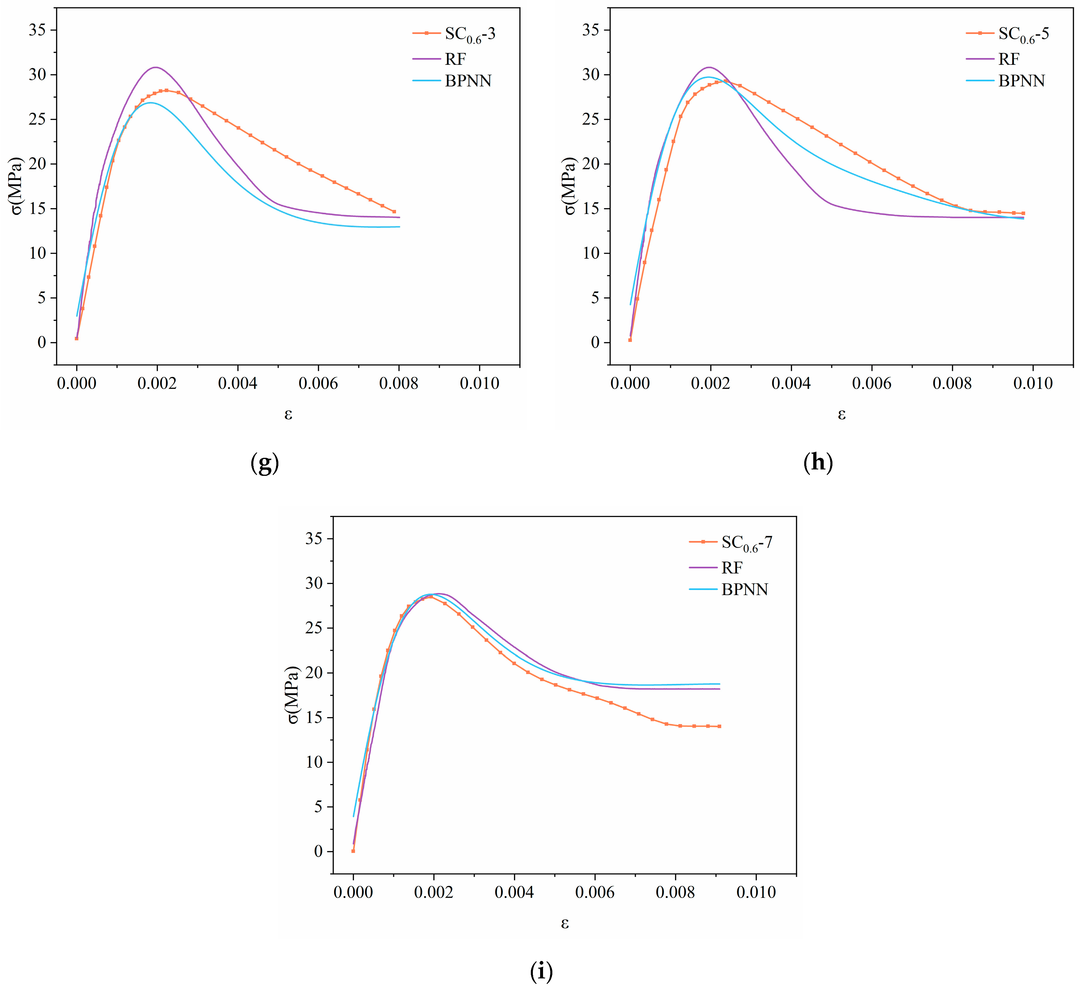
4.2. Prediction Results

Figure 16 shows the prediction results of the stress–strain relationship of steam-cured SC specimens with SA replacement ratios of 30%, 50%, and 70% by the RF and optimized BPNN prediction models. Meanwhile,

Table 4. Evaluation of the prediction results of the RF and BPNN models.

Specimens	Models	R2	MAE	RMSE
SC0.4-3	RF	0.6964	3.7321	5.0259
	BPNN	0.8262	2.8909	3.8029
SC0.4-5	RF	−0.8609	7.8362	9.7264
	BPNN	0.5315	4.2346	4.8801
SC0.4-7	RF	0.8122	2.7112	2.8596
	BPNN	0.8233	2.1961	2.7740
SC0.5-3	RF	0.8603	2.4646	2.6623
	BPNN	0.8671	1.8523	2.5975
SC0.5-5	RF	0.7764	3.0443	3.2559
	BPNN	0.9558	1.1254	1.4476
SC0.5-7	RF	0.6713	6.6785	8.0771
	BPNN	0.7766	5.0750	6.6589
SC0.6-3	RF	0.6342	3.1214	3.5023
	BPNN	0.4438	3.7704	4.3184
SC0.6-5	RF	0.5816	3.2714	3.9553
	BPNN	0.8886	1.6571	2.0408
SC0.6-7	RF	0.8322	1.9463	2.2727
	BPNN	0.8127	1.8592	2.4015

presents the statistical evaluation metrics of the RF and optimized BPNN models’ predictions of the stress–strain data of nine groups of steam-cured SC.

As shown in Figure 16, both RF and BPNN models can accurately capture the linear mechanical response in the ascending branch and the nonlinear behavior in the descending branch when predicting the stress–strain relationship of steam-cured SC with unknown mix proportions. However, the RF model generally overestimates the peak stress, indicating that its prediction of the uniaxial compressive strength of steam-cured SC is somewhat aggressive. From Figure 16 and Table 4, it can be seen that for the SC_0.6-7 specimen, the prediction performance of the two models is comparable (R² ≈ 0.822), with RF being slightly better; for the SC_0.6-3 specimen, the generalization ability of RF is significantly better than that of BPNN (R²: 0.634 vs 0.444); the prediction results for the remaining seven specimens show that the generalization ability of the BPNN model is superior to that of the RF model. The BPNN model is capable of capturing complex nonlinear relationships between input features and output variables. However, the complexity of these relationships varies across different mix ratios. SC_0.6-3 has simpler data relationships (with its descending segment being closer to linear), which do not require the full capacity of the BPNN model, leading to the poor performance of the BPNN. The BPNN model is highly sensitive to hyperparameters (such as the number of hidden layers, the number of neurons, and the learning rate). The hyperparameter settings of the BPNN that are effective for the concrete mix ratios in the training set may not perform well for a specific mix ratio in the test set. Table 4 shows that neither the RF nor the BPNN model performed well in predicting the stress–strain data of SC_0.4-5, SC_0.5-7, and SC_0.6-3. The RF model performed poorly in predicting SC_0.4-5 (R² = −0.861). The RF model, despite its strong robustness, may still fail to generalize effectively if it encounters data distributions that were not present in the training data. Similar to references [13,56], the SC with a 50% SA volume fraction exhibits unique mechanical properties, which is the turning point in the variation in the mechanical properties of SC. The SC_0.4-5 dataset contains rare cases that were not seen in the training data, leading to the poor predictive performance of the RF model. Additionally, the features used in the RF model do not have the same level of relevance across different concrete mix ratios. For SC_0.4-5, some features that are important in other datasets become less informative and may even be misleading. The RF model’s MAE and RMSE fluctuate significantly (e.g., RMSE = 8.077 for SC_0.5-7), indicating that the robustness of the RF model needs to be improved. The BPNN model has R² ≥ 0.8 for six groups of specimens, with the highest value reaching 0.956 (SC_0.5-5), and its MAE and RMSE values are generally lower than those of the RF model, showing better prediction stability for specimens with higher SA replacement ratios (such as SC_0.4-7 and SC_0.5-7).

A comprehensive comparison of the prediction results of the stress–strain relationship of steam-cured SC by the models shows that the BPNN model has stronger generalization ability when the SA volume replacement ratio changes, and its prediction stability is significantly better than that of the RF model. The excellent performance of the BPNN model indicates that it is more suitable for the extrapolation prediction of mix proportions in practical engineering and has a certain practical value. At the same time, compared with traditional theoretical uniaxial compressive stress–strain models [56], the generalization ability advantage of machine learning methods needs to be further verified through a wider range of test data, with particular attention to the impact of multi-factor coupling (such as curing system, mix proportion, and microstructure) on the prediction results.

5. Conclusions

With the help of test and machine learning algorithms, the stress–strain behaviors of steam-cured SC at 50 °C under uniaxial compression was studied. The theoretical basis for the efficient utilization of steel slag in precast concrete components was established, and the following conclusions are drawn:

(1)

Steam curing significantly enhances the mechanical properties of SC. The peak stress of the specimens is increased, the ultimate strain is raised, and the descending segment of the uniaxial compressive stress–strain curve of SC becomes more gentle. The peak stress of SC initially increases and then decreases with the rise in the SA volume replacement ratio, reaching its maximum when the SA replacement ratio is 40%. The main cracking surface of SC specimens under uniaxial compression failure is the side surface. Standard-cured specimens exhibit more pronounced brittle failure characteristics, while steam-cured specimens show more ductile failure modes.

(2)

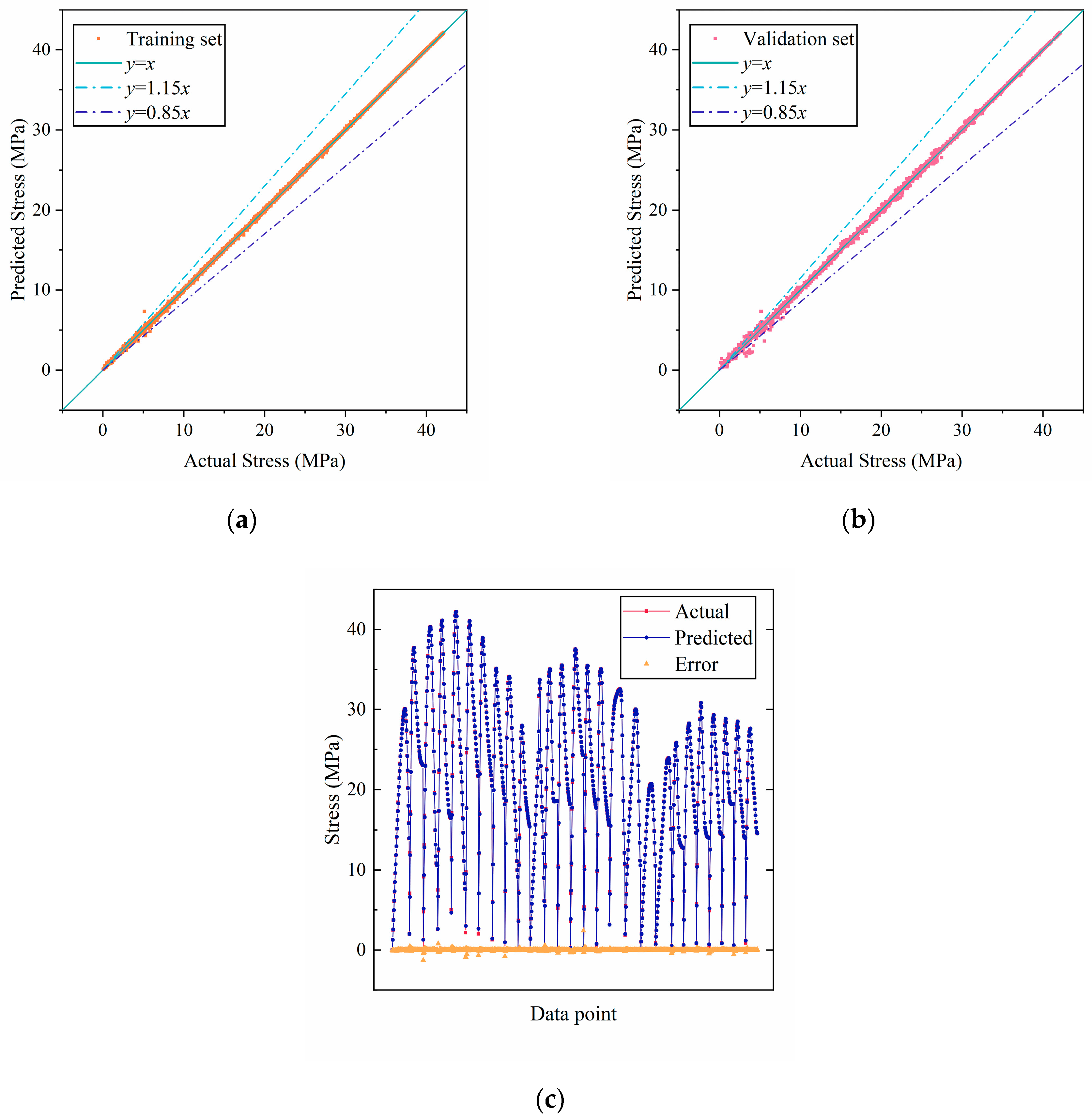
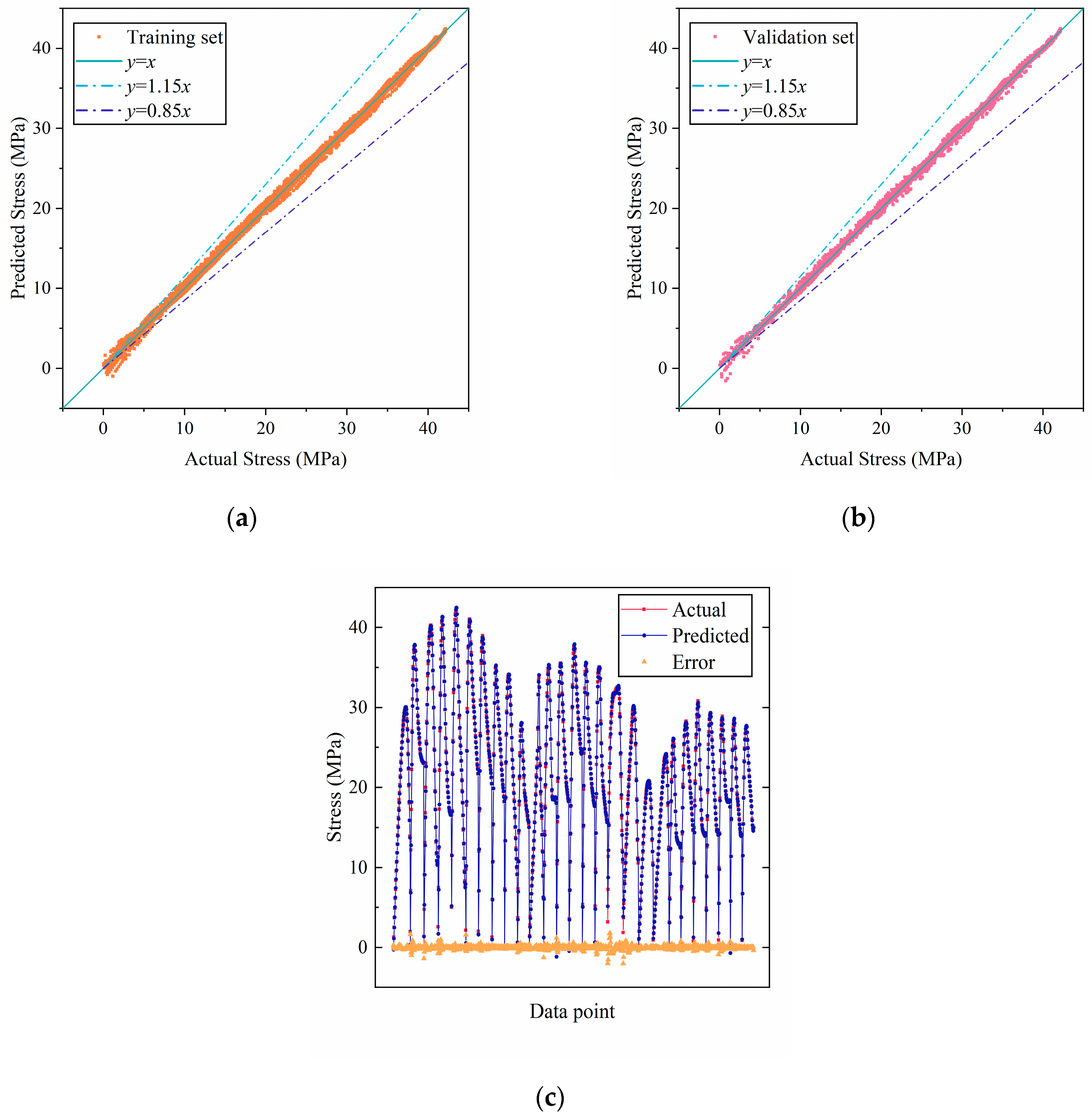
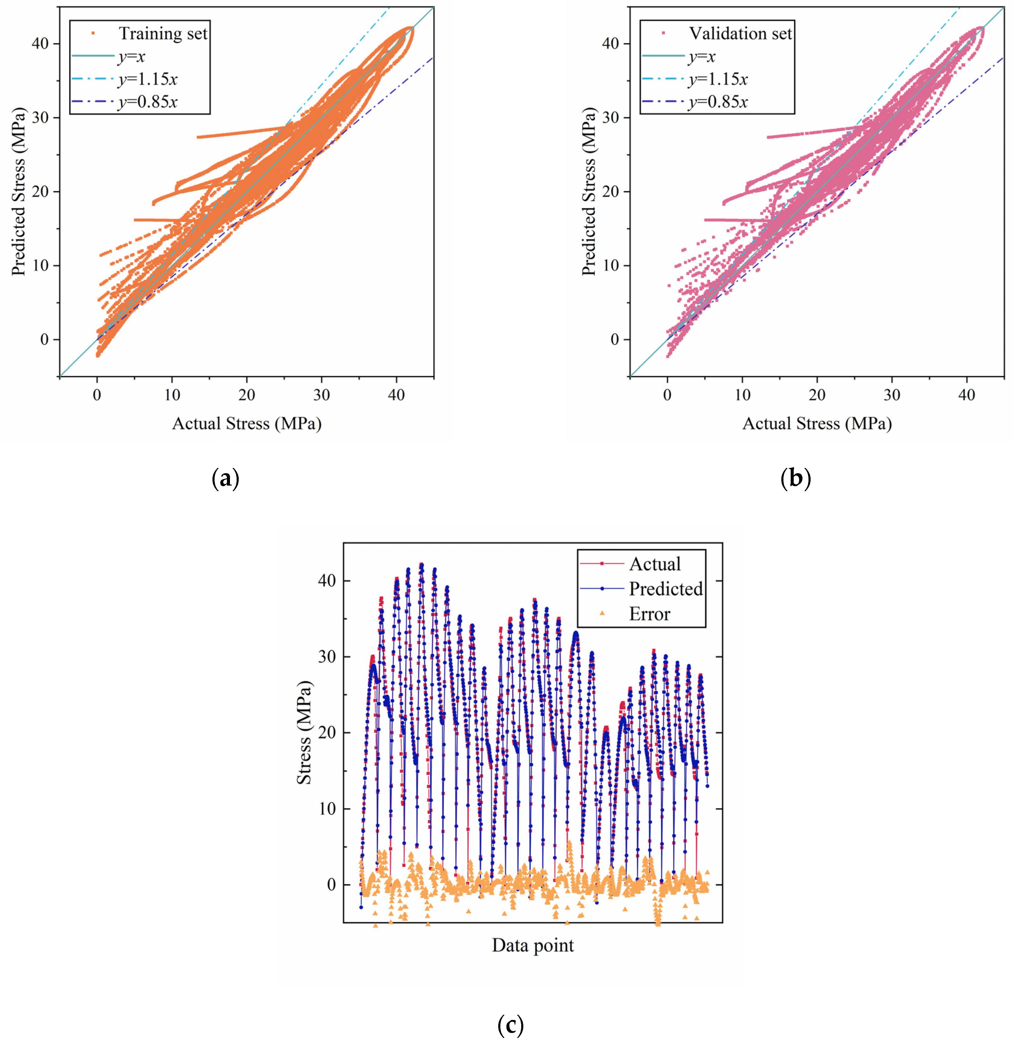
By artificial thinning and randomly dividing the uniaxial compressive stress–strain data of steam-cured SC, the prediction performance of the RF, BPNN, and SVR models was compared. It was found that the RF model performed the best (R² = 1.00), with over 95% of the data points falling within the ±15% error band. The BPNN model was the next best. However, the SVR model, due to its large prediction point dispersion and significant errors, is not suitable for this type of stress prediction (testing set R² = 0.943). The prediction results of the RF and BPNN models are in very good agreement with the test results.

(3)

The RF and BPNN models were reconstructed and rerun to test their generalization ability in predicting the stress–strain relationship of SC specimens across mix proportions. It was found that after optimization (reducing the number of hidden layer neurons from sixty-four to eight), the BPNN model showed enhanced stability in cross-content prediction, with an R² of 0.8 or higher for six groups of specimens and a peak value of 0.956. However, the RF model overestimated the peak stress when predicting the stress of SC specimens with untrained SA contents, indicating that its robustness needs improvement. Transfer learning validation showed that the BPNN model has the most engineering value, with prediction errors for SC with untrained contents of 30%, 50%, and 70% stably within 6 MPa. This validation method not only confirmed the BPNN model’s generalization capability across various mix proportions but also highlighted its practical utility in engineering applications.

References

1. Su, N.; Lou, L.; Amirkhanian, A.; Amirkhanian, S.N.; Xiao, F. Assessment of Effective Patching Material for concrete Bridge Deck—A Review. Constr. Build. Mater. 2021, 293, 123520. [Google Scholar] [CrossRef]
2. Tang, S.W.; Yao, Y.; Andrade, C.; Li, Z.J. Recent Durability Studies on Concrete Structure. Cem. Concr. Res. 2015, 78, 143–154. [Google Scholar] [CrossRef]
3. Khan, M.; Rehman, A.; Ali, M. Efficiency of Silica-Fume Content in Plain and Natural Fiber Reinforced Concrete for Concrete Road. Constr. Build. Mater. 2020, 244, 118382. [Google Scholar] [CrossRef]
4. Shamass, R.; Limbachiya, V.; Ajibade, O.; Rabi, M.; Lopez, H.U.L.; Zhou, X. Carbonated Aggregates and Basalt Fiber-Reinforced Polymers: Advancing Sustainable Concrete for Structural Use. Buildings 2025, 15, 775. [Google Scholar] [CrossRef]
5. Al-Kheetan, M.J.; Jweihan, Y.S.; Rabi, M.; Ghaffar, S.H. Durability Enhancement of Concrete with Recycled Concrete Aggregate: The Role of Nano-ZnO. Buildings 2024, 14, 353. [Google Scholar] [CrossRef]
6. Guo, J.; Bao, Y.; Wang, M. Steel Slag in China: Treatment, Recycling, and Management. Waste Manag. 2018, 78, 318–330. [Google Scholar] [CrossRef]
7. Dong, Q.; Wang, G.; Chen, X.; Tan, J.; Gu, X. Recycling of Steel Slag Aggregate in Portland Cement Concrete: An Overview. J. Clean. Prod. 2021, 282, 124447. [Google Scholar] [CrossRef]
8. Rashad, A.M. Behavior of Steel Slag Aggregate in Mortar and Concrete—A Comprehensive Overview. J. Build. Eng. 2022, 53, 104536. [Google Scholar] [CrossRef]
9. Guo, Y.; Xie, J.; Zheng, W.; Li, J. Effects of Steel Slag as Fine Aggregate on Static and Impact Behaviours of Concrete. Constr. Build. Mater. 2018, 192, 194–201. [Google Scholar] [CrossRef]
10. Qasrawi, H.; Shalabi, F.; Asi, I. Use of Low CaO Unprocessed Steel Slag in Concrete as Fine Aggregate. Constr. Build. Mater. 2009, 23, 1118–1125. [Google Scholar] [CrossRef]
11. Xue, G.; Fu, Q.; Xu, S.; Li, J. Macroscopic Mechanical Properties and Microstructure Characteristics of Steel Slag Fine Aggregate Concrete. J. Build. Eng. 2022, 56, 104742. [Google Scholar] [CrossRef]
12. Fu, Q.; Xue, G.; Xu, S.; Li, J.; Dong, W. Mechanical Performance, Microstructure, and Damage Model of Concrete Containing Steel Slag Aggregate. Struct. Concr. 2022, 24, 2189–2207. [Google Scholar] [CrossRef]
13. Guo, Y.; Xie, J.; Zhao, J.; Zuo, K. Utilization of Unprocessed Steel Slag as Fine Aggregate in Normal- and High-Strength Concrete. Constr. Build. Mater. 2019, 204, 41–49. [Google Scholar] [CrossRef]
14. Chen, Z.; Huang, L.; Yan, L.; Li, S.; Cai, H.; Li, Y.; Luo, X. Characterising Mechanical Properties and Failure Criteria of Steel Slag Aggregate Concrete under Multiaxial Stress States. Constr. Build. Mater. 2024, 424, 135903. [Google Scholar] [CrossRef]
15. Wang, Q.; Yan, P. Hydration Properties of Basic Oxygen Furnace Steel Slag. Constr. Build. Mater. 2010, 24, 1134–1140. [Google Scholar] [CrossRef]
16. Belhadj, E.; Diliberto, C.; Lecomte, A. Properties of Hydraulic Paste of Basic Oxygen Furnace Slag. Cem. Concr. Compos. 2014, 45, 15–21. [Google Scholar] [CrossRef]
17. Shi, C.; Hu, S. Cementitious Properties of Ladle Slag Fines under Autoclave Curing Conditions. Cem. Concr. Res. 2003, 33, 1851–1856. [Google Scholar] [CrossRef]
18. Zhou, Z.; Jin, Q.; Hu, D.; Zhu, L.; Li, Z.; Su, W. Long-term Volume Stability of Steel Slag Sand Mortar and Concrete. Case Stud. Constr. Mater. 2025, 22, e04179. [Google Scholar] [CrossRef]
19. Feng, P.; Li, Z.; Zhang, S.; Yang, J.Q. Steel Slag Aggregate Concrete Filled-In FRP Tubes: Volume Expansion Effect and Axial Compressive Behaviour. Constr. Build. Mater. 2022, 318, 125961. [Google Scholar] [CrossRef]
20. Cai, Y.; Gao, S.; Wang, F.; Zhang, Z.; Zhao, Z.; Ma, B. Early Hydration Heat Temperature Field of Precast Concrete T-Beam under Steam Curing: Experiment and Simulation. Case Stud. Constr. Mater. 2023, 18, e02067. [Google Scholar] [CrossRef]
21. Shao, Y.; Zhang, Z.; Liu, X.; Zhu, L.; Han, C.; Li, S.; Du, W. Comprehensive Utilization of Industry By-Products in Precast Concrete: A Critical Review from the Perspective of Physicochemical Characteristics of Solid Waste and Steam Curing Conditions. Materials 2024, 17, 4702. [Google Scholar] [CrossRef] [PubMed]
22. Duan, Y.; Wang, Q.; Long, Z.; Wang, X. Investigating the Impact of Fly Ash on the Strength and Micro-Structure of Concrete during Steam Curing and Subsequent Stages. Materials 2023, 16, 1326. [Google Scholar] [CrossRef]
23. GB/T 37439-2019; Precast Post-Tensioned Prestressed Concrete Simply-Supported Beam of High-Speed Railway. Chinese Standard Press: Beijing, China, 2019. (In Chinese)
24. Li, H.; Lin, J.; Zhao, D.; Shi, G.; Wu, H.; Wei, T.; Li, D.; Zhang, J. A BFRC Compressive Strength Prediction Method Via Kernel Extreme Learning Machine-Genetic Algorithm. Constr. Build. Mater. 2022, 344, 128076. [Google Scholar] [CrossRef]
25. Sarfarazi, S.; Mascolo, I.; Modano, M.; Guarracino, F. Application of Artificial Intelligence to Support Design and Analysis of Steel Structures. Metals 2025, 15, 408. [Google Scholar] [CrossRef]
26. Jweihan, Y.S.; Al-Kheetan, M.J.; Rabi, M. Empirical Model for the Retained Stability Index of Asphalt Mixtures Using Hybrid Machine Learning Approach. Appl. Syst. Innov. 2023, 6, 93. [Google Scholar] [CrossRef]
27. Rabi, M. Bond Prediction of Stainless-Steel Reinforcement Using Artificial Neural Networks. Proc. Inst. Civ. Eng.-Constr. Mater. 2023, 2, 177. [Google Scholar] [CrossRef]
28. Shang, H.; Wu, P.; Lou, Y.; Wang, J.; Chen, Q. Machine Learning-Based Modeling of the Coupling Effect of Strain Rate and Temperature on Strain Hardening for 5182-O Aluminum Alloy. J. Mater. Process. Technol. 2022, 302, 117501. [Google Scholar] [CrossRef]
29. Li, X.; Roth, C.C.; Mohr, D. Machine-Learning Based Temperature- and Rate-Dependent Plasticity Model: Application to Analysis of Fracture Experiments on DP Steel. Int. J. Plast. 2019, 118, 320–344. [Google Scholar] [CrossRef]
30. Zhou, M.; Ye, G.; Yuen, K.V.; Yu, W.; Jin, Q. A Graph Attention Reasoning Model for Prefabricated Component Detection. Comput.-Aided Civ. Infrastruct. Eng. 2025, 40, 13373. [Google Scholar] [CrossRef]
31. Ye, G.; Yuen, K.V.; Jin, Q.; Zhou, M.; Yin, C.; Jiang, Q.; Zhao, S.; Su, W. Evaluation Method for Uniformity of Steel Slag Concrete Aggregate Based on Improved YOLOv8. J. Build. Eng. 2024, 73, 111046. [Google Scholar] [CrossRef]
32. Sun, Y.; Cheng, H.; Zhang, S.; Mohan, M.K.; Ye, G.; De Schutter, G. Prediction & Optimization of Alkali-Activated Concrete Based on the Random Forest Machine Learning Algorithm. Constr. Build. Mater. 2023, 385, 131519. [Google Scholar] [CrossRef]
33. Kim, T.K.; Hwang, S.-H.; Kim, J.; Jung, W.-T.; Yoon, J. Analysis of Bond Strength of CFRP Cables with Concrete Using Random Forest Model. J. Build. Eng. 2024, 96, 110658. [Google Scholar] [CrossRef]
34. Dada, T.E.; Gong, G.; Xia, J.; Sarno, L.D. Stress-Strain Behaviour of Axially Loaded FRP-Confined Natural and Recycled Aggregate Concrete Using Design-Oriented and Machine Learning Approaches. J. Build. Eng. 2024, 95, 110256. [Google Scholar] [CrossRef]
35. Zheng, C.; Liu, Y.; Li, L.; Yang, L. Effect of Sulfate Freeze-Thaw on the Stress-Strain Relationship of Recycled Coarse Aggregate Self-Compacting Concrete: Experimental and Machine Learning Algorithms. Constr. Build. Mater. 2024, 449, 138383. [Google Scholar] [CrossRef]
36. GB 175-2007; Common Portland Cement. National Standards of the People’s Republic of China: Beijing, China, 2007. (In Chinese)
37. JGJ 55-2011; Specification for Mix Proportion Design of Ordinary Concrete. National Standards of the People’s Republic of China: Beijing, China, 2011. (In Chinese)
38. GB/T 50081-2019; Standard for Test Methods of Concrete Physical and Mechanical Properties. National Standards of the People’s Republic of China: Beijing, China, 2019. (In Chinese)
39. Allen, D.H.; Searcy, C.R. A Micromechanical Model for a Viscoelastic Cohesive Zone. Int. J. Fract. 2001, 107, 159–176. [Google Scholar] [CrossRef]
40. Masad, E.; Castelo Branco, V.T.F.; Little, D.N.; Lytton, R. A Unified Method for the Analysis of Controlled-Strain and Controlled-Stress Fatigue Testing. Int. J. Pavement Eng. 2008, 9, 233–246. [Google Scholar] [CrossRef]
41. Zhou, K.; Lei, D.; He, J.; Zhang, P.; Bai, P.; Zhu, F. Real-Time Localization of Micro-Damage in Concrete Beams Using DIC Technology and Wavelet Packet Analysis. Cem. Concr. Compos. 2021, 123, 104198. [Google Scholar] [CrossRef]
42. Wang, X.; Liu, J.; Jin, Z.; Chen, F.; Zhong, P.; Zhang, L. Real-Time Strain Monitoring of Reinforced Concrete under the Attacks of Sulphate and Chloride Ions Based on XCT and DIC Methods. Cem. Concr. Compos. 2022, 125, 104314. [Google Scholar] [CrossRef]
43. Guo, J.; Gao, S.; Liu, A.; Wang, H.; Guo, X.; Xing, F.; Zhang, H.; Qin, Z.; Ji, Y. Experimental Study on Failure Mechanism of Recycled Coarse Aggregate Concrete under Uniaxial Compression. J. Build. Eng. 2023, 63, 105548. [Google Scholar] [CrossRef]
44. Xue, G.; Fu, Q.; Zhou, H.; Sun, L. Experimental Study on Stress-Strain Relationship of Steel Slag Fine Aggregate Concrete under Uniaxial Compression. J. Southwest Jiaotong Univ. 2022, 57, 1165–1174. (In Chinese) [Google Scholar] [CrossRef]
45. Breiman, L. Random forests. Mach. Learn. 2001, 45, 5–32. [Google Scholar] [CrossRef]
46. Wu, Y.; Peng, S.; Xie, Q.; Xu, P. Nonlinear Least Squares with Local Polynomial Interpolation for Quantitative Analysis of IR Spectra. Spectrochim. Acta Part A Mol. Biomol. Spectrosc. 2019, 206, 147–153. [Google Scholar] [CrossRef] [PubMed]
47. Coelho, A.A. Optimum Levenberg–Marquardt Constant Determination for Nonlinear Least-Squares. J. Appl. Crystallogr. 2018, 51, 428–435. [Google Scholar] [CrossRef]
48. Petrović, M.; Rakočević, V.; Kontrec, N.; Panić, S.; Ilić, D. Hybridization of Accelerated Gradient Descent Method. Numer. Algorithms 2018, 79, 769–786. [Google Scholar] [CrossRef]
49. Yuvaraj, P.; Murthy, A.R.; Iyer, N.R.; Sekar, S.; Samui, P. Support Vector Regression Based Models to Predict Fracture Characteristics of High Strength and Ultra High Strength Concrete Beams. Eng. Fract. Mech. 2013, 98, 29–43. [Google Scholar] [CrossRef]
50. Myers, R.H. Classical and Modern Regression with Applications, 2nd ed.; Duxbury Press: Belmont, CA, USA, 2000. [Google Scholar]
51. Lai, S.; Serra, M. Concrete Strength Prediction by Means of Neural Network. Constr. Build. Mater. 1997, 11, 93–98. [Google Scholar] [CrossRef]
52. Feng, D.C.; Liu, Z.T.; Wang, X.D.; Chen, Y.; Chang, J.Q.; Wei, D.F.; Jiang, Z.M. Machine Learning-Based Compressive Strength Prediction for Concrete: An Adaptive Boosting Approach. Constr. Build. Mater. 2020, 230, 117000. [Google Scholar] [CrossRef]
53. Duan, J.; Asteris, P.G.; Nguyen, H.; Bui, X.-N.; Moayedi, H. A Novel Artificial Intelligence Technique to Predict Compressive Strength of Recycled Aggregate Concrete Using ICA-XGBoost Model. Eng. Comput. 2021, 37, 3329–3346. [Google Scholar] [CrossRef]
54. Chou, J.S.; Pham, A.D. Enhanced Artificial Intelligence for Ensemble Approach to Predicting High Performance Concrete Compressive Strength. Constr. Build. Mater. 2013, 49, 554–563. [Google Scholar] [CrossRef]
55. Cheng, M.Y.; Chou, J.S.; Roy, A.F.V.; Wu, Y.W. High-Performance Concrete Compressive Strength Prediction Using Time-Weighted Evolutionary Fuzzy Support Vector Machines Inference Model. Autom. Constr. 2012, 28, 106–115. [Google Scholar] [CrossRef]
56. Wang, C.; Ye, G.; Jin, Q.; Zhou, Z.; Hu, D.; Wei, Y. The Uniaxial Compressive Stress-Strain Relations of Steel Slag Fine Aggregate Concrete under Steam Curing. Constr. Build. Mater. 2025, 459, 139820. [Google Scholar] [CrossRef]
Figure 1. Particle size distribution of SA, natural stone, and natural sand.
Buildings 15 01817 g001
Figure 2. Procedure for fabricating and curing SC specimens.
Buildings 15 01817 g002
Figure 3. Steam curing system.
Buildings 15 01817 g003
Figure 4. SC uniaxial compressive stress–strain curve testing method. (a) The main hardware equipment of the XTDIC-3D non-contact full-field strain measurement system; (b) the stress–strain test system for SC under uniaxial compression; and (c) the stress–strain tests procedure for SC.
Buildings 15 01817 g004aBuildings 15 01817 g004b
Figure 5. Workflows diagram of the RF model.
Buildings 15 01817 g005
Figure 6. BPNN prediction model structure diagram.
Buildings 15 01817 g006
Figure 7. SVR prediction model. (a) Schematic diagram of the principle of SVR; (b) schematic diagram of the structure of the SVR prediction model.
Buildings 15 01817 g007
Figure 8. Typical uniaxial compression failure main fracture surfaces of SC specimens. (a) SC0.4-6; (b) SC0.4-10; (c) SC0.5-1; (d) SC0.5-5; (e) SC0.6-2; (f) SC0.6-4; (g) SC0.5-5b; and (h) SC0.5-6b.
Buildings 15 01817 g008
Figure 9. The 28-day uniaxial compressive stress–strain curve of SC: (a) 0.4 water–cement ratio steam-cured SC; (b) 0.5 water–cement ratio steam-cured SC; (c) 0.6 water–cement ratio steam-cured SC; and (d) 0.5 water–cement ratio standard-cured SC.
Buildings 15 01817 g009
Figure 10. Results of the RF stress–strain prediction model. (a) Scatter plot of predicted vs. actual values for the training set; (b) scatter plot of predicted vs. actual values for the validation set; and (c) errors of predicted vs. actual values for the testing set.
Buildings 15 01817 g010
Figure 11. Results of the BPNN stress–strain prediction model. (a) Scatter plot of predicted vs. actual values for the training set; (b) scatter plot of predicted vs. actual values for the validation set; and (c) errors of predicted vs. actual values for the testing set.
Buildings 15 01817 g011
Figure 12. Results of the SVR stress–strain prediction model. (a) Scatter plot of predicted vs. actual values for the training set; (b) scatter plot of predicted vs. actual values for the validation set; and (c) errors of predicted vs. actual values for the testing set.
Buildings 15 01817 g012
Figure 13. The stress prediction results of steam-cured SC with the water–cement ratio of 0.4 by the three models. (a) SC0.4-0; (b) SC0.4-1; (c) SC0.4-2; (d) SC0.4-3; (e) SC0.4-4; (f) SC0.4-5; (g) SC0.4-6; (h) SC0.4-7; and (i) SC0.4-10.
Buildings 15 01817 g013aBuildings 15 01817 g013b
Figure 14. The stress prediction results of steam-cured SC with the water–cement ratio of 0.5 by the three models. (a) SC0.5-0; (b) SC0.5-1; (c) SC0.5-2; (d) SC0.5-3; (e) SC0.5-4; (f) SC0.5-5; (g) SC0.5-6; (h) SC0.5-7; and (i) SC0.5-10.
Buildings 15 01817 g014aBuildings 15 01817 g014b
Figure 15. The stress prediction results of steam-cured SC with the water–cement ratio of 0.6 by the three models. (a) SC0.6-0; (b) SC0.6-1; (c) SC0.6-2; (d) SC0.6-3; (e) SC0.6-4; (f) SC0.6-5; (g) SC0.6-6; (h) SC0.6-7; and (i) SC0.6-10.
Buildings 15 01817 g015aBuildings 15 01817 g015b
Figure 16. The prediction results of the RF and BPNN models for the stress of steam-cured SC with untrained mix proportion. (a) SC0.4-3; (b) SC0.4-5; (c) SC0.4-7; (d) SC0.5-3; (e) SC0.5-5; (f) SC0.5-7; (g) SC0.6-3; (h) SC0.6-5; and (i) SC0.6-7.
Buildings 15 01817 g016aBuildings 15 01817 g016b