1. Introduction
The rational utilization of natural ventilation can significantly reduce the substantial energy consumption in industrial buildings due to the diverse environmental control demands they often face. In China, industrial buildings accounted for over 7% of the annual national primary energy consumption, with approximately 50–55% being dedicated to heating, ventilation, and air conditioning (HVAC) systems for maintaining acceptable in-door environmental conditions [
1]. Natural ventilation enables outdoor air infiltration and air exchange without energy consumption, thereby substantially decreasing the operational energy requirements for mechanical ventilation and cooling systems in buildings [
2].
However, the airflow in industrial buildings under natural ventilation conditions is influenced by both internal building conditions and the outdoor environment, exhibiting complex and variable patterns [
3]. In industrial production, the vertical arrangement of processing technology commonly leads to the use of multi-layer vertically connected plants. Material is processed from top to bottom and output through multiple stages, and the sources of heat are continuously stabilized in the upper layers of the plant. There is a vertically connected space inside this type of plant that facilitates the handling of materials and equipment, as well as the maintenance of the production system. Due to the complex internal conditions, it is difficult to determine the airflow pattern of this type of plant under the effect of natural ventilation, which poses significant challenges in indoor thermal environment control and pollutant dispersion, resulting in an inability to scientifically optimize the plant environment under natural ventilation. Therefore, it is imperative to investigate airflow patterns and ventilation effectiveness strategies in such buildings under natural ventilation.
Under natural ventilation, airflow can be driven by the thermal pressure caused by the density difference induced by a temperature difference, or it could be ascribed to the wind pressure distribution caused by an outdoor airflow acting on building surfaces [
4]. Thermal pressure mainly originates due to temperature differences and effective elevation differences between openings. The distribution of wind pressure not only depends on natural climate conditions, such as outdoor wind speed and direction, but is also related to the building itself and the structural characteristics of the architectural complex where it is located [
5]. In practice, airflow patterns emerge from the coupled effects of these drivers, exhibiting complex nonlinear interactions [
6]. Airflow states are influenced by multiple factors.
Extensive research has been conducted on the airflow in buildings under different natural ventilation conditions. Some scholars have analyzed the characteristics of natural convection flow under the conditions of different architectural geometric structures and classified the main forms of above-ground buildings as single-zone single-opening [
7], single-zone double-opening [
8,
9,
10,
11], single-zone multi-opening [
12,
13,
14,
15,
16], double-zone multi-opening buildings [
17,
18] and multi-zone multi-opening buildings. Studies on multi-zone natural ventilation have focused on buildings that can be broadly categorized into two types, according to the arrangement of the zones: horizontally or vertically oriented (i.e., multi-layer buildings) [
19]. Wang et al. [
20] explored the flow of air inside each room of a three-layer civil building under natural ventilation and analyzed air exchange through windows between non-directly connected rooms. In multi-story buildings with structures such as stacks, each floor of the building is connected to the stack through small openings. Moreover, in such buildings, there is often a backflow prevention design, which largely prevents the cross-layer flow of air among floors. Shi et al. [
21] designed a model of a three-story building with a stack structure under buoyancy-driven natural ventilation where airflow enters the room through the bottom windows of each floor and then flows into the stack structure through the higher openings and then out of the top openings. Beyond above-ground structures, some scholars have also conducted in-depth studies on airflow in underground structures such as tunnels [
22,
23] and underground hydropower stations [
24] under natural ventilation conditions.
In addition to the geometric structure of a building, the outside environment also has a significant impact on the natural convection flow characteristics inside the building. Therefore, many scholars have explored the characteristics of natural convection flow un-der different outdoor environmental conditions, such as indoor and outdoor temperature differences [
25,
26,
27], varying outdoor wind speeds [
28,
29], and varying outdoor wind directions [
30,
31,
32]. Wang et al. modeled a cavity with a solar chimney with CFD numerical simulation to investigate the indoor airflow and the performance effect of the solar chimney under the influence of different external wind conditions; they showed that the external wind not only induced the inflow of air through the window openings, but also enhanced the performance of the solar chimney by reducing the air resistance. Some scholars also took into account the non-uniform and transient characteristics of the actual atmospheric environment, as well as outdoor temperature gradients [
33], outdoor wind frequency [
34], and other climate environmental spatiotemporal change characteristics. Thebault et al. conducted an in-depth study on the influence of outdoor thermal stratification on natural convection flow patterns and mass flow in an open vertical channel by combining experiments and numerical simulation. Studies have shown that, in addition to outdoor atmospheric conditions, other environ-mental conditions around the building, such as surrounding infrastructure including factories [
35], adjacent buildings [
36], and even surrounding trees [
37] and viaducts [
38], also have a certain impact on the natural ventilation flow in the indoor building environment. Finally, Zhong et al. studied the influence of the size of a single upstream building and the gap between two upstream buildings on the internal airflow and ventilation rate of the target building under natural ventilation. The above studies have advanced our understanding of the flow characteristics of natural ventilation in various buildings under different conditions, and have important guiding significance for the rational use of natural ventilation and the realization of an efficient and low-consumption ventilation design.
However, in multi-layer vertically connected plants, the existence of space inside the building that connects the floors to each other may lead to the mixing of airflow among the floors of the plant. Furthermore, compared with civil buildings, industrial buildings are often equipped with a variety of medium–high-intensity heat sources, on which outdoor thermal pressure and wind pressure are superimposed, resulting in a large difference in internal airflow between industrial buildings and civil buildings [
39]. When considered with the effect of natural thermal and wind pressure, the natural convection flow is complex and changeable, and the vector characteristics of the driving force prevent the direct superposition of multiple driving forces when they work together. Thus, in existing research, the airflow patterns inside multi-layer vertically connected plants when outdoor thermal pressure and wind pressure are applied have not yet been determined.
Therefore, in this study, CFD numerical simulation is used to explore the influence of applying outdoor thermal and wind pressure on the airflow patterns in a plant of this type.
2. Methodology
2.1. Geometrical Model and Computational Domain
CFD has been one of the most promising approaches in natural ventilation research and design over the past few decades [
40,
41,
42]. In this study, CFD numerical simulation was carried out to computationally investigate the airflow patterns inside a multi-layer vertically connected plant with heat sources, and the influence of outdoor thermal and wind pressure on the airflow pattern inside the plant is clarified.
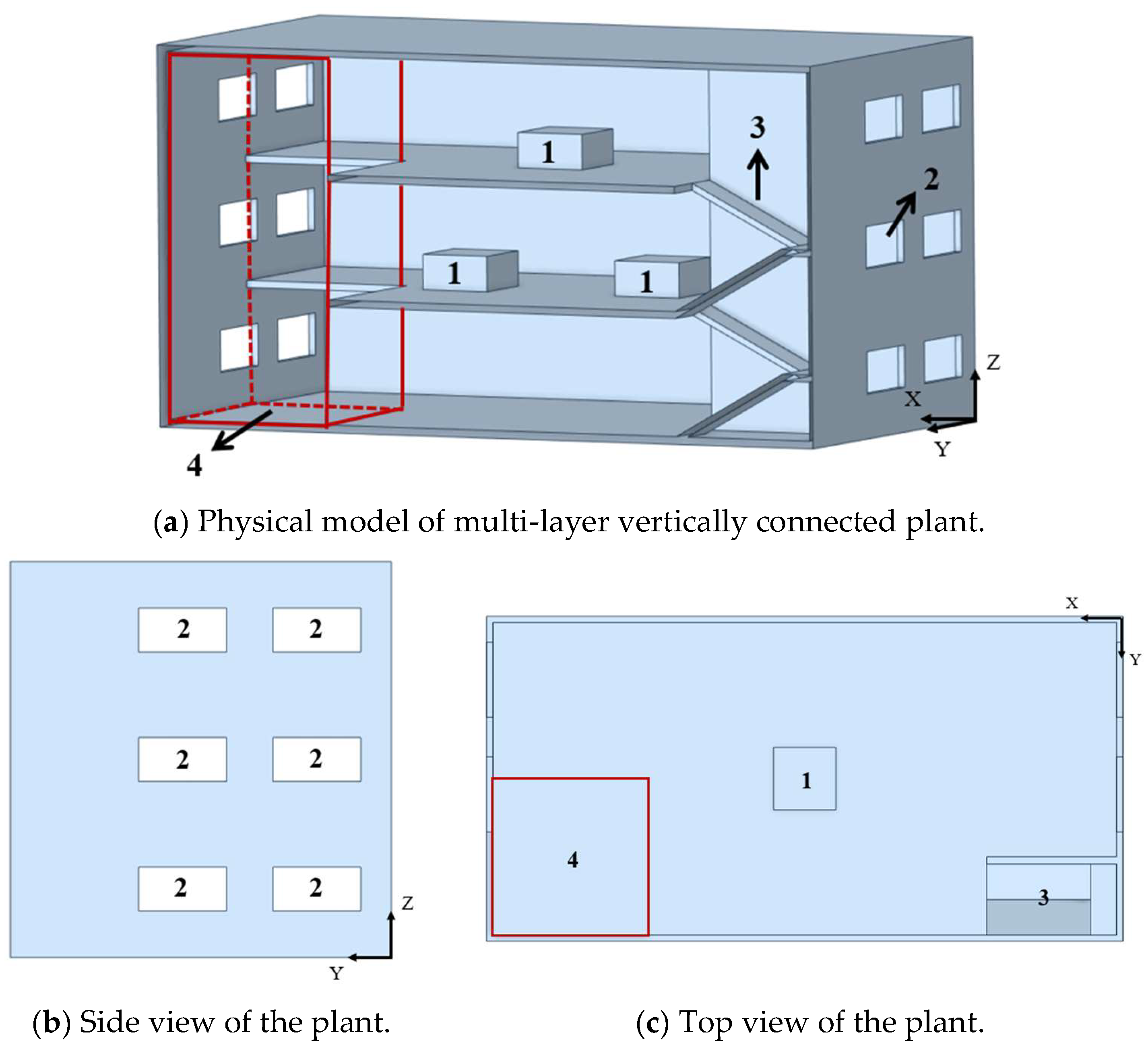
Figure 1 shows the physical model of a multi-layer vertically connected plant, which was created by using a three-dimensional calculation model based on the dimensions of an actual multi-layer carbon anode production plant for aluminum electrolysis. The dimensions of the plant were rationalized and simplified for ease of study and analysis. This type of plant in the industrial production activities, the processing equipment arranged on upper floors of the plant will produce a certain amount of heat, and in the natural ventilation conditions, the air temperature difference caused by the thermal equipment in the plant is a driving force for air flow. Therefore, in this modeling study, we considered the layout of the heat sources on the various floors according to the actual production processes of this type of plant. The plant model dimensions were
L ×
W ×
H = 30.6 m × 15.6 m × 16.2 m, and those of a single heat source were
Ls ×
Ws ×
Hs = 3 m × 3 m × 1.5 m. There is usually a silo at the top of this type of plant to supply multiple production processes; the spacing between two heat sources arranged on the same floor was 1.5 m. The dimensions of the vertically connected structure were
Lc ×
Wc ×
Hc = 7.5 m × 7.5 m × 16.2 m, and the opening of the stairwell measured
Lf ×
Wf ×
Hf = 7.5 m × 3.7 m × 16.2 m. In this study, the windows were considered to be fully open. Therefore, the specific window shape of the opening was not modeled to simplify computations. Moreover, due to the large number of windows in the actual plant, on the basis of ensuring equal window-to-wall ratios, two windows in close proximity to each other were merged into a single window during modeling to facilitate the analysis. The dimensions of a single window were set to
Lw ×
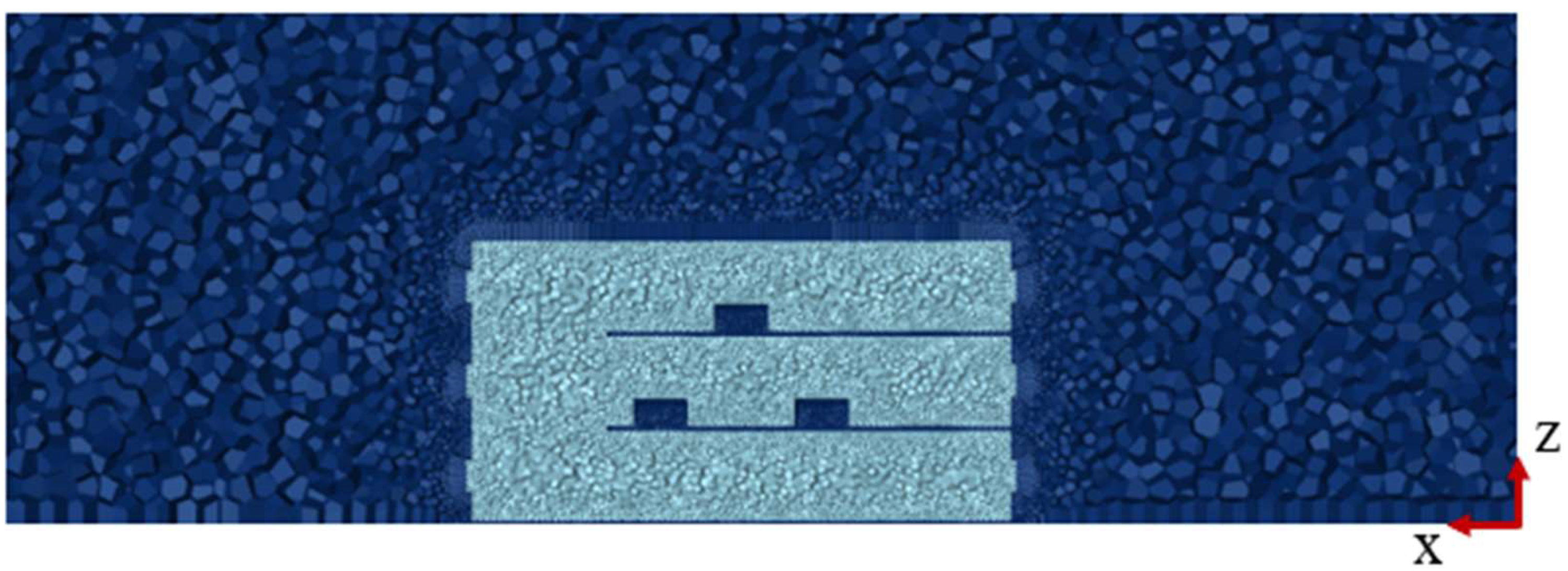
Hw = 3.6 m × 1.8 m, and the space between two windows was 1.9 m. The window arrangement induces cross-ventilation during wind simulations. When the outdoor wind blows through the plant, a backflow area will be formed on the lee side of the plant, and the flow in the backflow area is more complicated, which may cause window air intake and exhaust air on the lee side of the plant. Therefore, the lifting of the outdoor wind around the upper edge of the building and the backflow formed on the lee side must be fully considered when determining the calculation domain. Moreover, the computational domain dimensions significantly influence the accuracy of the numerical calculation results. Therefore, the computational domain of the numerical simulation was appropriately enlarged in order to more accurately study the influence of the outdoor atmospheric environment on the airflow pattern in the factory building as follows [
43]: the lengths on the windward and leeward sides were set to be 5 and 10 times the height of the plant, respectively, and the calculation height was 8 times the height of the plant, as shown in
Figure 2.
2.2. Grid-Sensitivity Analysis
ANSYS Fluent 2022R1 Meshing was employed for grid generation. Given the extensive computational domain, we used a coarser grid with a maximum size of 1.50 m for the external domain and a smaller grid with a maximum size of 0.12 m for the internal domain. Boundary layer meshes with wall refinement were implemented, and hexahedral elements were utilized throughout. The mesh configuration is illustrated in
Figure 3.
Grid quality and density critically influence the accuracy of the numerical simulation of a flow field, so it is necessary to verify the independence of the grid. Three mesh resolutions were evaluated: for grid independence verification, which were 4.96 million, 8.20 million and 11.71 million grids, respectively.
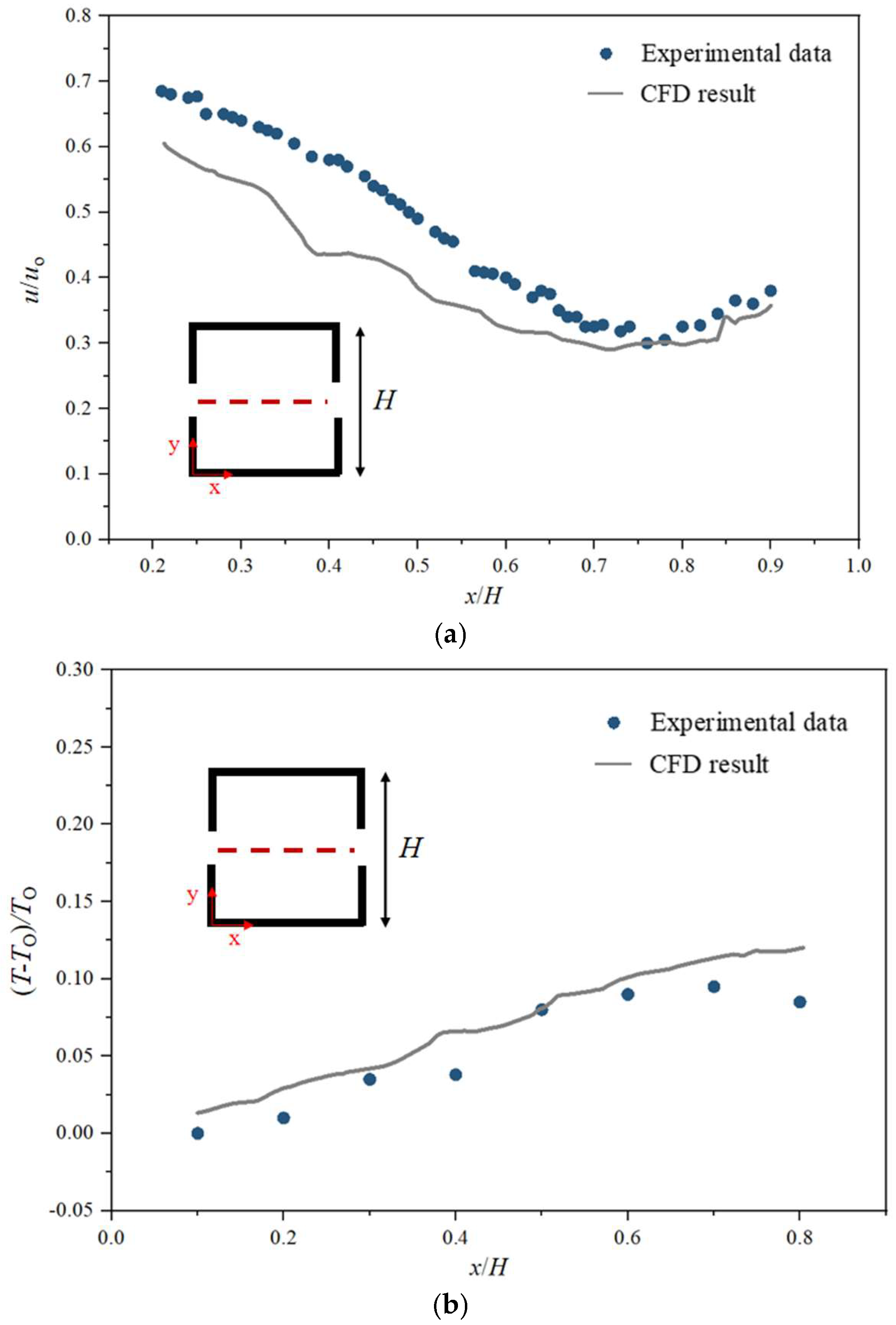
Figure 4a shows the comparison diagram of dimensionless velocity changes with
x/
L on the horizontal measuring line (
y/
H = 0.50,
z/
H = 0.18) in the center of the window on the ground floor of the plant under different grid quantities. A reference velocity of 1 m/s was considered for the outdoor incoming wind speed during calculation.
Figure 4b shows the comparison of temperature changes with
h/
H on the vertical line of the center of the plant vertically connected space for different grid numbers (
y/
H = 0.74,
x/
H = 1.72). It can be found that the calculation results of 8.20 million and 11.71 million grid cells are basically the same and that the temperature predictions showed <1% relative error, while the velocity discrepancies remained within 5%. Therefore, all simulations in this study were calculated by using a grid cell number of 8.20 million.
2.3. Selection of Turbulence Models and Boundary Conditions
When using Fluent for calculation, a pressure-based solver was selected, and open the Gravity model (Gravity), Energy model (Energy) and viscosity model (Viscous). Among the turbulence numerical simulation methods, Reynolds Averaged Navier–Stokes (RANS) has been widely used in natural ventilation research [
44]; for example, for predicting airflow and pollutant diffusion. The solution time of RANS is greatly shortened compared with Large Eddy Simulation (LES) and Direct Numerical Simulation (DNS). The two-equation turbulence model
is the most widely used turbulence model due to its strong generality, few restrictive conditions, and high computational stability [
45]. It has been found that when simulating airflow in naturally ventilated buildings, the calculations using the RNG
model are in better agreement with the test results compared to the standard
[
46]. Therefore, we employ the turbulence model RNG
for calculation. The governing equations are shown below.
Energy equation:
where
p is the pressure (Pa),
T is the temperature (K),
μ is the dynamic viscosity (Pa·s),
Pr is the Prandtl number,
Prt is the turbulent Prandtl number (
Prt = 0.85),
St is the heat source term (W/(m
3·s)),
ρ is the density (kg/m
3),
k is the turbulent kinetic energy,
ε is the turbulent dissipation rate,
gi is the acceleration due to gravity (m/s
2),
ui is the time-averaged velocity (m/s),
uj denotes the velocity components (m/s), and for the RNG
k −
ε model, the model constant
Cμ = 0.0845.
In order to make the equations closed, equations about turbulent kinetic energy k and dissipation rate ε are introduced, respectively. For the RNG k-ε model, the equations k and equations ε obtained are as follows:
Equations
ε:
where
Gk represents the generation term of turbulent kinetic energy due to the average velocity gradient, where
,
μt is the turbulent viscosity
,
,
, and the model constant
,
,
,
,
,
.
It is assumed that air is an incompressible gas, and we adopt the Boussinesq hypothesis for the density change caused by temperature differences. In addition to the buoyancy term in the dynamic equation, the density is considered to be constant. The ideal gas equation of state is introduced to obtain closed-form equations:
where
ρ represents the density of air (kg/m
3),
R is the constant of ideal gases (J/(mol·K),
T is the air temperature (K),
M is the molar mass of air (g/mol), and
p is the pressure (Pa).
The turbulence model selected above is only suitable for fully developed turbulence. In the near-wall region, the flow condition changes greatly and requires specialized near-wall treatment. Therefore, the wall function method is used to solve the problem of the inaccurate calculation of the turbulence model near the wall. The enhanced wall treatment (EWT) combines the two-layer low-Reynolds-number model and the enhanced wall function. If the mesh near the wall is dense enough , the two-layer model corrects the turbulent viscosity in the equation. The flow and heat transfer in the viscous bottom layer can be accurately solved. Therefore, the enhanced wall treatment method is used in this study to process the airflow near the wall.
The boundary conditions were specified as follows: When the simulation calculation was carried out without applying outdoor thermal and wind pressure or by only applying outdoor thermal pressure, pressure boundary conditions were set at both the inlet and outlet of the plant. The temperature at the heat source was set to be maintained at a certain level according to the processes of the plant. For the heat sources arranged in the plant, we adopted the first type of boundary conditions, and the surface temperature of the heat sources was set to 373.15 K. The indoor ambient temperature was set to 298.15 K. When we applied outdoor wind pressure in the simulation calculation, the boundary condition of the flow inlet of the outdoor basin was set as the velocity inlet boundary, and the wind speed was set to a uniform velocity. Outflow boundary conditions were used at the exit of the external computational domain. In this study, the thermal conductivity of the wall was ignored, and the wall conditions were all set to adiabatic.
We adopted the SIMPLEC algorithm for the coupling of pressure and speed in the simulation calculation, and the pressure difference was set to ‘PRESTO!’. The momentum, energy, k and ε equations are all in the second-order upwind format. Check the residuals values (momentum, continuity, turbulence, etc.: the residuals need to be reduced to less than 1 × 10⁻³, and energy equations: the residuals need to be reduced to less than 1 × 10⁻⁶), monitor whether the physical quantities have reached a stable level or not (the physical quantities fluctuation is less than 1%, which is considered to be convergence) and check whether the mass flux is conserved (the difference between the inlet and outlet fluxes needs to be less than 0.1% of the total flux) to ensure the calculation has converged under different work conditions.
2.4. CFD Model Validation
In order to verify the reliability of the numerical model of natural ventilation airflow field in this paper, the airflow velocity and temperature data provided in the wind tunnel experiments conducted by Kosutova et al. [
47] were used in this study. They investigate the internal airflow of a single building with two opposing side windows and a heated internal heat source under natural ventilation conditions. The influence of the outdoor atmosphere was taken into account to investigate the changes in air velocity and temperature inside the building under the influence of the incoming outdoor wind. In this study, the airflow inside the plant is mainly driven by the temperature difference caused by the internal arrangement of heat sources and the outdoor atmospheric environment. Therefore, it is reasonable to use the experiments selected in the paper for the validation of the numerical models.
In the wind tunnel experiments, the dimensions of the wind tunnel test section were 0.9 × 0.6 × 4.5 m
3, and those of the model in the wind tunnel were 1.5 × 1.5 × 1.5 m
3 (
L ×
W ×
H). The large-opening case (with 12% façade porosity) was chosen for validation. Two-dimensional PIV measurements were carried out to measure the air velocity, and their uncertainty was around 1–5.5%. NTC U-type sensors with a diameter of 2.4 mm and a precision of 0.05 °C were used to measure the indoor air temperature. Note that experimental predictions of turbulent kinetic energy near openings are unreliable. More specific parameters of the test rig and detailed experimental procedures can be found in the literature [
47].
The computational model used for model validation matches the dimensions of the wind tunnel experiments in the literature (large-opening case). The first height of the partition grid near the wall was 2 × 10⁻⁴ m, and the value of y+ was about 3. The turbulence model was RNG , and the enhanced wall treatment was selected for the processing of near-wall flow. The inlet boundary conditions were set to velocity inlet, the outlet boundary conditions to outflow, the outdoor wind speed uo at a height of 0.15 m is set to 1.90 m/s, and the outdoor temperature To is set to 25.5 °C. The wind direction was perpendicular to the facade opening, and the temperature of the heating wall inside the building was set to 60 °C. The other walls were set to be under adiabatic boundary conditions.
Figure 5a,b compare the dimensionless flow velocity components and dimensionless temperature as a function of
x/
H on the measured line obtained with the experiment and the numerical simulation, respectively. In this study, the main focus is on the overall airflow in the plant and does not explore the details of the localized flow of airflow in the vicinity of the window. Therefore, we take the middle segment for validation. Except for the values near the openings, the trends of the parameter distributions under simulated and experimental conditions are basically the same. The maximum error of the measured speed, 24.70%, is at
x/
H = 0.38. The maximum error of the measured temperature is only 4.67%, at
x/
H = 0.9. Therefore, it is considered that the CFD model in this study is acceptable and can accurately predict the airflow in the plant under the action of wind pressure and outdoor thermal pressure.
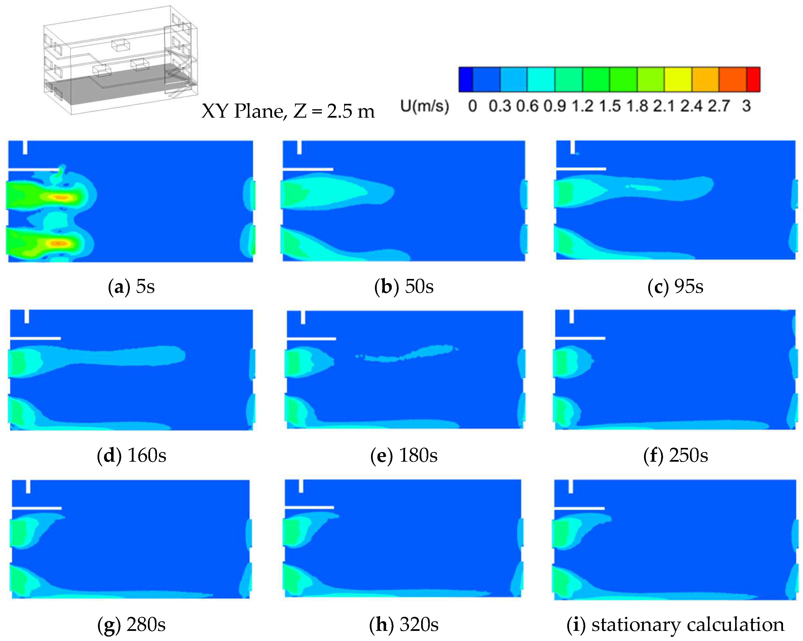
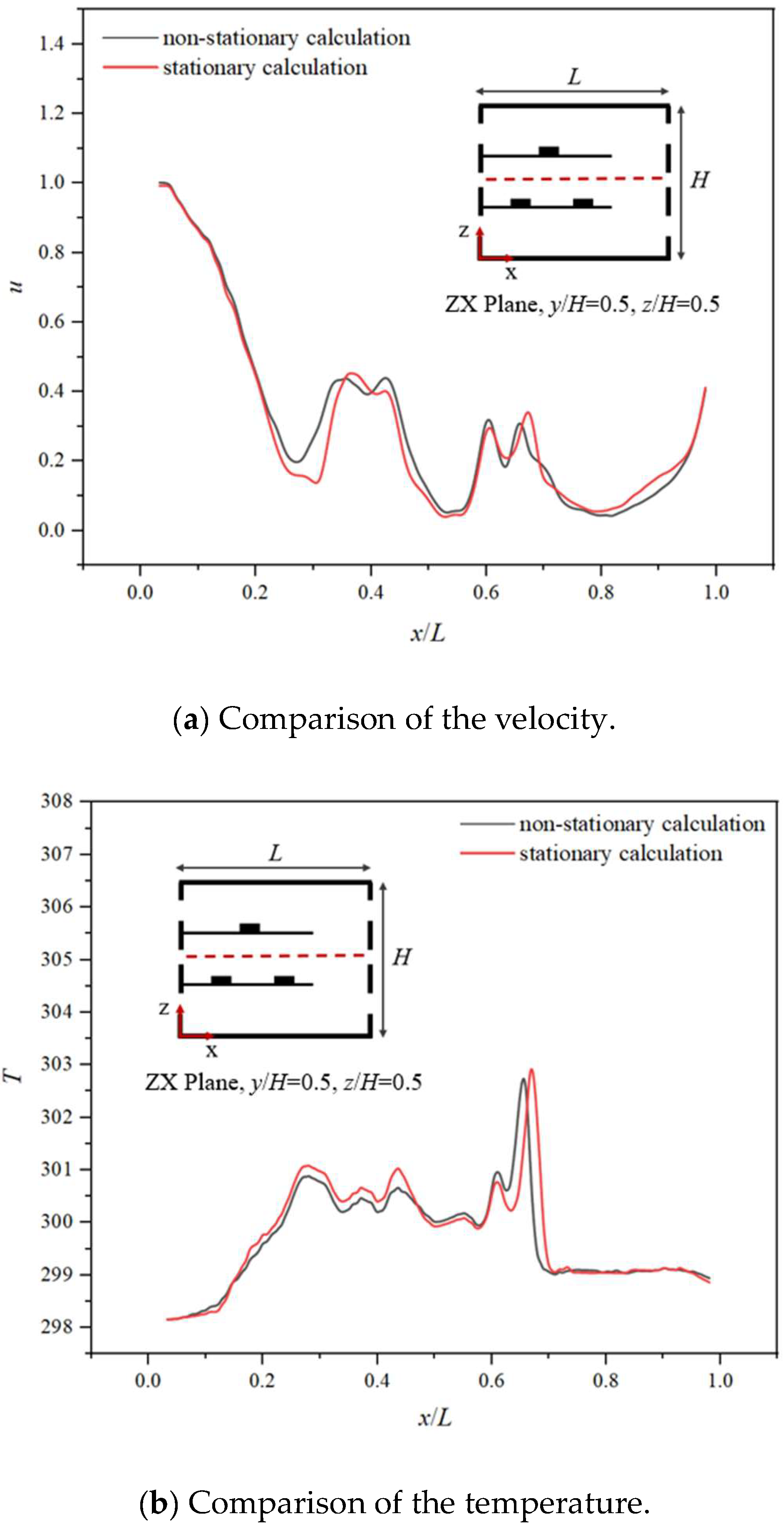
In order to verify the accuracy of the stationary calculation model in this paper, we conducted a non-static modeling when the airflow is driven by a combination of heat pressure and wind pressure (Outdoor wind speed is 1 m/s and outdoor air temperature is 298.15 K). We have compared the velocity and temperature derived from the non-stationary model with the results of the stationary calculation. As shown in
Figure 6, it can be found that the relatively stable velocity field formed after a certain time step of non-stationary modeling is basically consistent with the stationary calculation.
Figure 7a,b show the velocity and temperature change on the measuring line in the middle layer of the plant, and it can be found that the speed and temperature values derived from the stationary calculation are basically the same as those of the non-stationary calculation. This paper investigates the relative stability state of airflow in the plant long after the unsteady state phase. The use of stationary calculation can save a lot of computational time and resources. Therefore, this paper adopts the stationary calculation in the investigation.
2.5. Setting of Simulated Conditions
We first determined and analyzed the airflow characteristics caused by the heat sources in the multi-layer vertically connected plant under the conditions of no outdoor wind nor thermal pressure. On this basis, the influence of outdoor thermal and wind pressure on the airflow pattern was then investigated.
Five cities with the considered type of plant from five thermal climate zones were selected to extract the outdoor design parameters for the characterization of thermal and wind pressure effects. The dry-bulb temperature and mean wind speed calculated for the winter and summer ventilation in each city are presented in
Table 1. In winter, there are large differences in the design temperature of outdoor ventilation among cities and be-tween indoor and outdoor environments, while both these differences are minimal in summer. Therefore, for the selection of the outdoor thermal pressure conditions in this study, we considered the winter conditions, with large temperature difference between indoor and outdoor environments. It can be found from
Table 1 that the mean outdoor wind speed in winter and summer in the five cities with this type of plant spans 0–4 m/s, which was thus chosen as the outdoor wind speed (
uo) range in this study.
The heat source temperature was fixed at 373.15 K based on industrial processing requirements. The Grashof number of the heat source (
) is introduced with the following calculation formula:
where
g represents the gravitational acceleration (m/s
2),
is the coefficient of thermal expansion (1/K),
Ts is the temperature of the heat source (K),
Ti is the temperature of the indoor air (K),
H is the characteristic length (here, it refers to the height of the plant) (m), and
υ is the kinematic viscosity coefficient (m
2/s).
For the convenience of subsequent analysis, the Grashof number of outdoor thermal pressure (Gri−o) is introduced to explore the influence of outdoor thermal pressure on the airflow in the plant as follows:
where
To is the temperature of the outdoor air (K).
Various steps are involved in the determination of the influence of outdoor wind pressure on the existing airflow and ventilation effect in a plant, summarized as follows: consider the specific outdoor wind direction, that is, the air supply along the non-vertically connected side of the plant; set different outdoor wind speeds; and observe the changes in the airflow in the plant under different outdoor wind pressure intensities. In this study, the outdoor wind speed (
uo) was set to 0–4 m/s. The natural ventilation Reynolds number (
Reo) is introduced to facilitate the analysis of the calculated results:
where
uo is the outdoor wind speed (m/s).
The Grashof number of the heat sources (
Grs) in the plant remains unchanged at 4.3 × 10
13. The difference in temperature between indoor and outdoor environments de-creases with the increase in the outdoor air temperature, and the Grashof number of out-door thermal pressure (
Gri−o) decreases. With the increase in applied outdoor wind speed, the natural ventilation Reynolds number (
Reo) increases. The set conditions are shown in
Table 2. The conditions of Case 6 (i.e., no outdoor thermal and wind pressure) are used as the main reference comparison conditions to explore the influence of outdoor thermal and wind pressure of different intensities on airflow.
3. Results and Discussion
3.1. Analysis of Airflow Pattern in Multi-Layer Vertically Connected Plant with No Outdoor Thermal and Wind Pressure
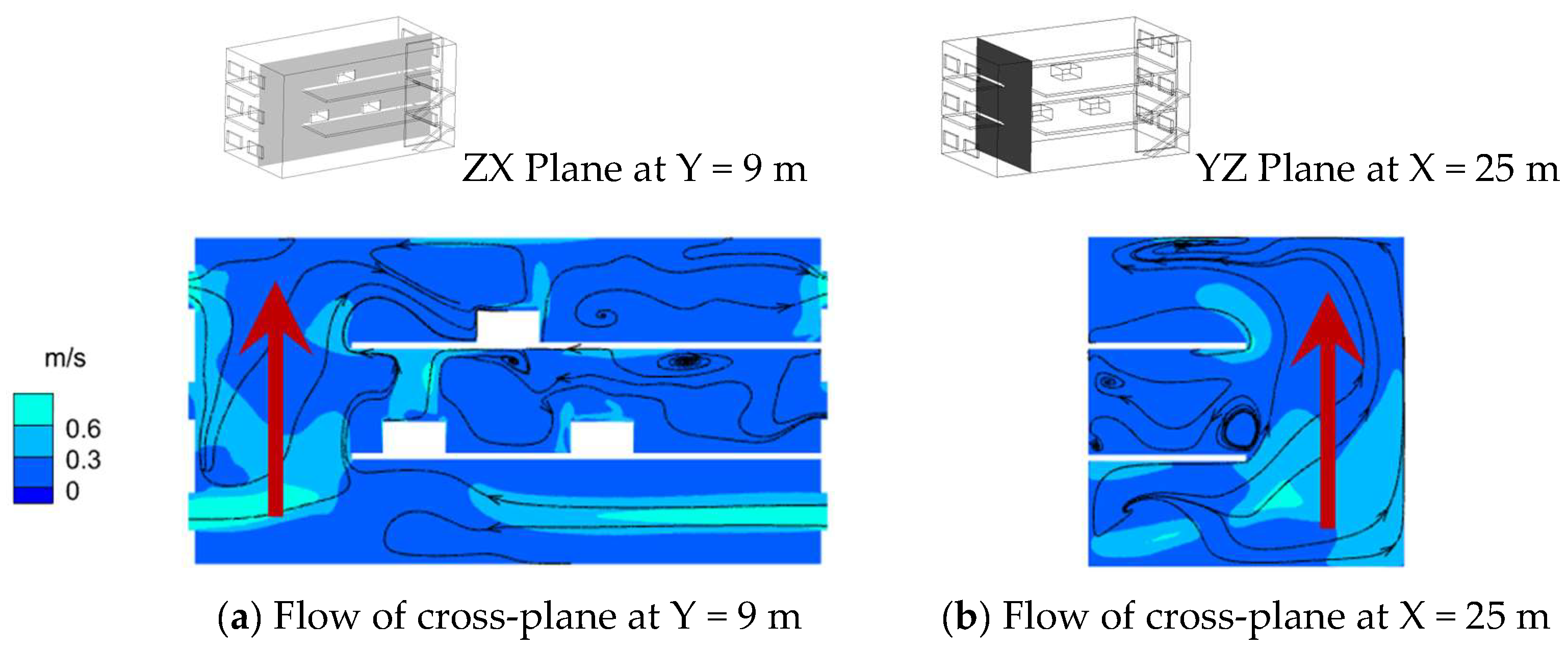
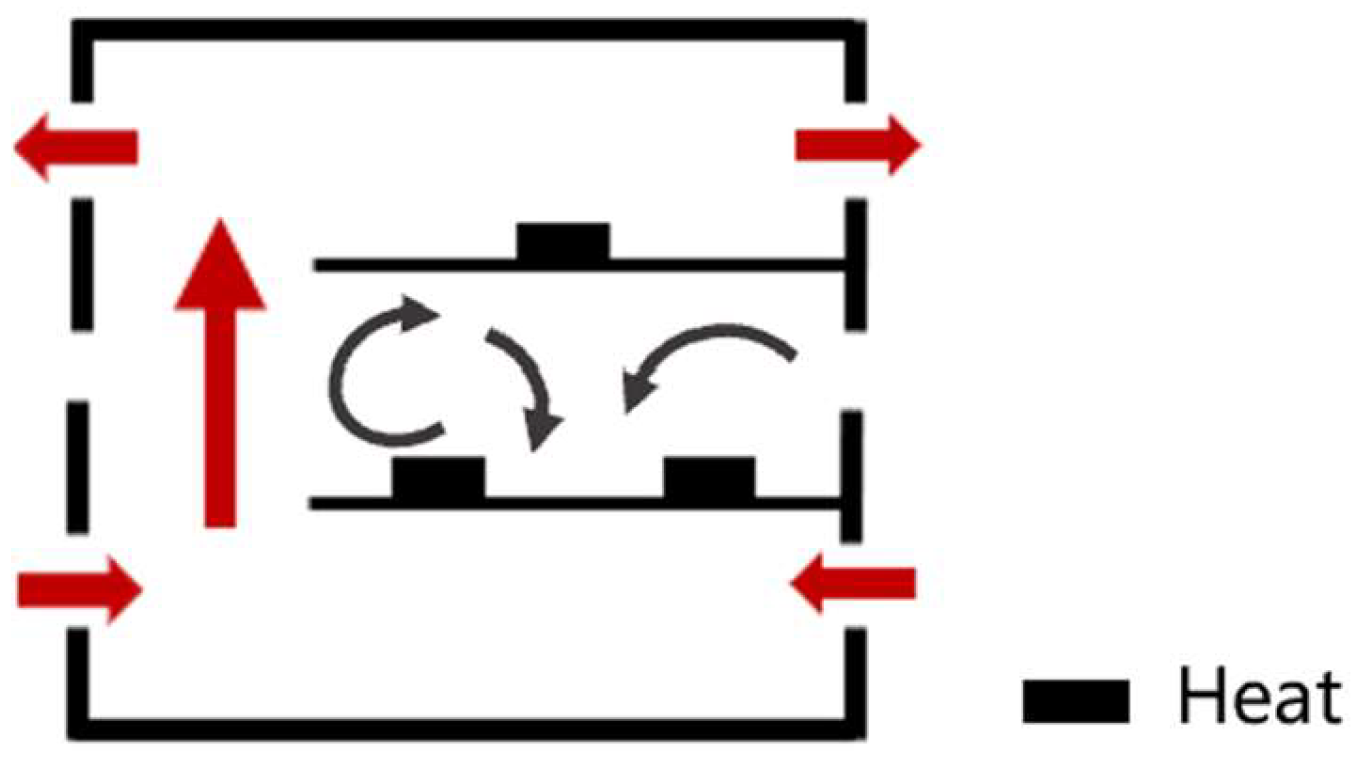
Figure 8 illustrates the flow diagram and velocity cloud diagram of the ZX section at Y = 9 m and the YZ section at X = 25 m of the plant when outdoor wind and thermal pressure are not applied (Case 6:
Gri−o = 0 and
Reo = 0). It can be found that without considering the influence of outdoor wind and thermal pressure, the airflow inside the plant is driven by the multiple heat sources arranged indoors; the outdoor air enters the plant through the windows on both sides of the ground floor and flows upward along the vertically connected space to the top floor of the plant, forming a flow of air from the bottom floor to the top floor. This cross-layer flow prevents the mesosphere airflow from merging with the overall flow, and the hot gas flow formed by the mesosphere tends to remain in the middle layer. From this, it can be concluded that when outdoor wind and thermal pressure are not applied to the plant, the indoor air forms flow pattern A: the air in the plant flows from the bottom layer to the top layer, and the middle-layer air does not merge with the overall flow (FP-A: overall upward, intermediate layer alone). The flow pattern diagram is shown in
Figure 9.
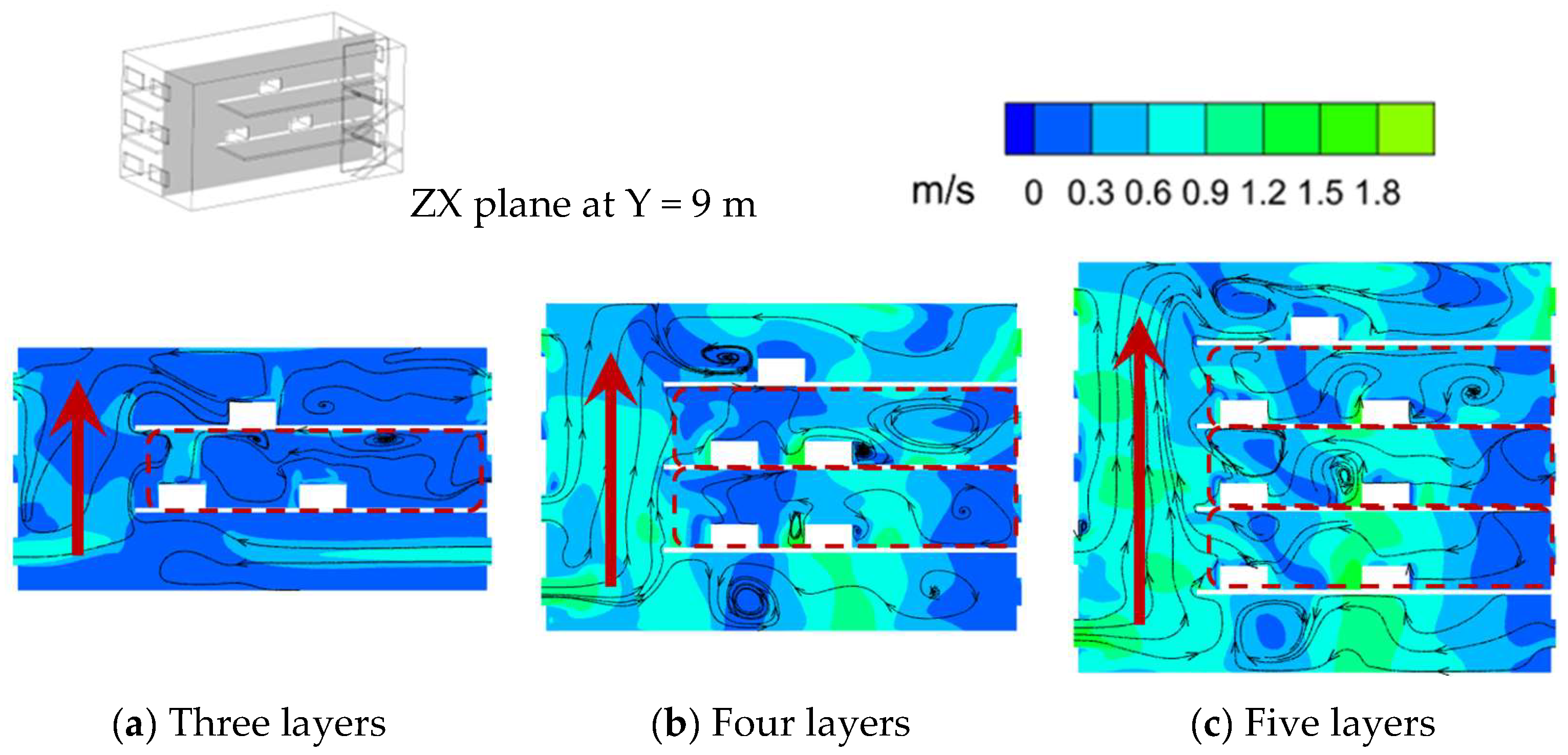
The number of layers of the plant was changed by increasing the number of intermediate floors, so as to investigate the effect of the number of floors on the indoor airflow pat-tern.
Figure 10 gives the flow line diagram and velocity cloud for the ZX section at Y = 9 m when the plant has three, four, and five layers. It is found that when the number of layers is increased from three to four and five, the outdoor air still enters the plant from the bottom window and flows upward along the vertically connected space to the top layer, forming a cross-stage cross-layer flow from the bottom to the top of the plant, and the airflow in the intermediate layer tends to remain within the layers. It can be found from the velocity cloud diagram that when the number of layers of a multi-layer vertically connected plant is increased from three to four or five, the airflow velocity at each layer is increased due to the increase in thermal pressure. In summary, it can be found that in a plant where the number of layers is increased from three to four or five, the airflow pattern does not change. Moreover, the number of floors in this type of plant is generally three or more according to the requirements of the production process. Therefore, the remainder of this study focused on the exploration of the influence of other factors on the airflow pat-tern in the plant on the basis of a three-layer plant.
3.2. Effect of Outdoor Thermal Pressure on Airflow in Plant
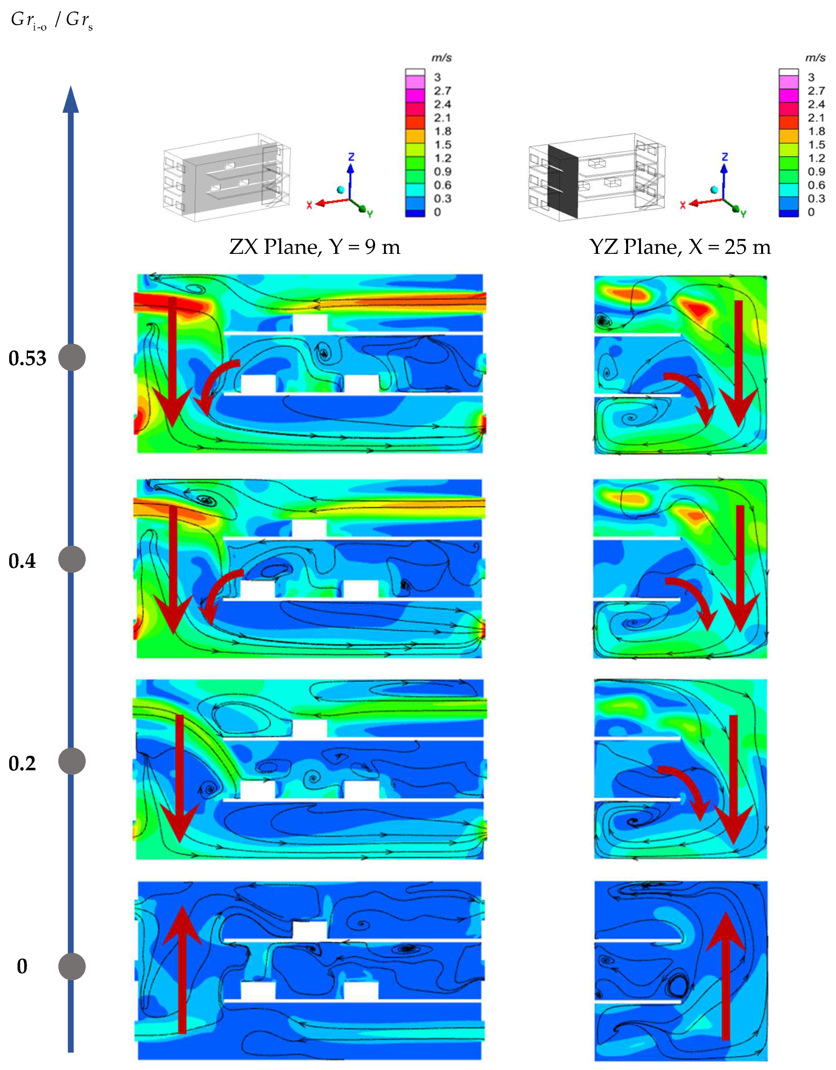
Outdoor thermal pressure at different strengths was applied to the plant, and
Figure 11 shows the flow diagram and velocity contours for the ZX cross-section at Y = 9 m and the YZ cross-section at X = 25 m. When the effect of outdoor thermal pressure is applied, the air flow is jointly driven by the indoor heat source and the outdoor thermal pressure. It can be found that when the ratio of the Glashof number of outdoor thermal pressure to that of the heat sources (
Gri−o/
Grs) increases from 0 to 0.20, the airflow pattern changes: the outdoor air, instead of entering the plant from the ground floor and flowing through the vertically connected space to the top floor, flows into the plant through the windows on both sides of the top floor and flows down the vertically connected space to the bottom floor, from where it finally flows out through the windows on the two sides. In addition, it can be found from the flow diagram of the X = 25 m section that when
Gri−o/
Grs = 0.20, the hot gas flow in the middle layer also converges to the vertically connected space and flows to the bottom of the plant along with the overall downward airflow. Therefore, when
Gri−o/
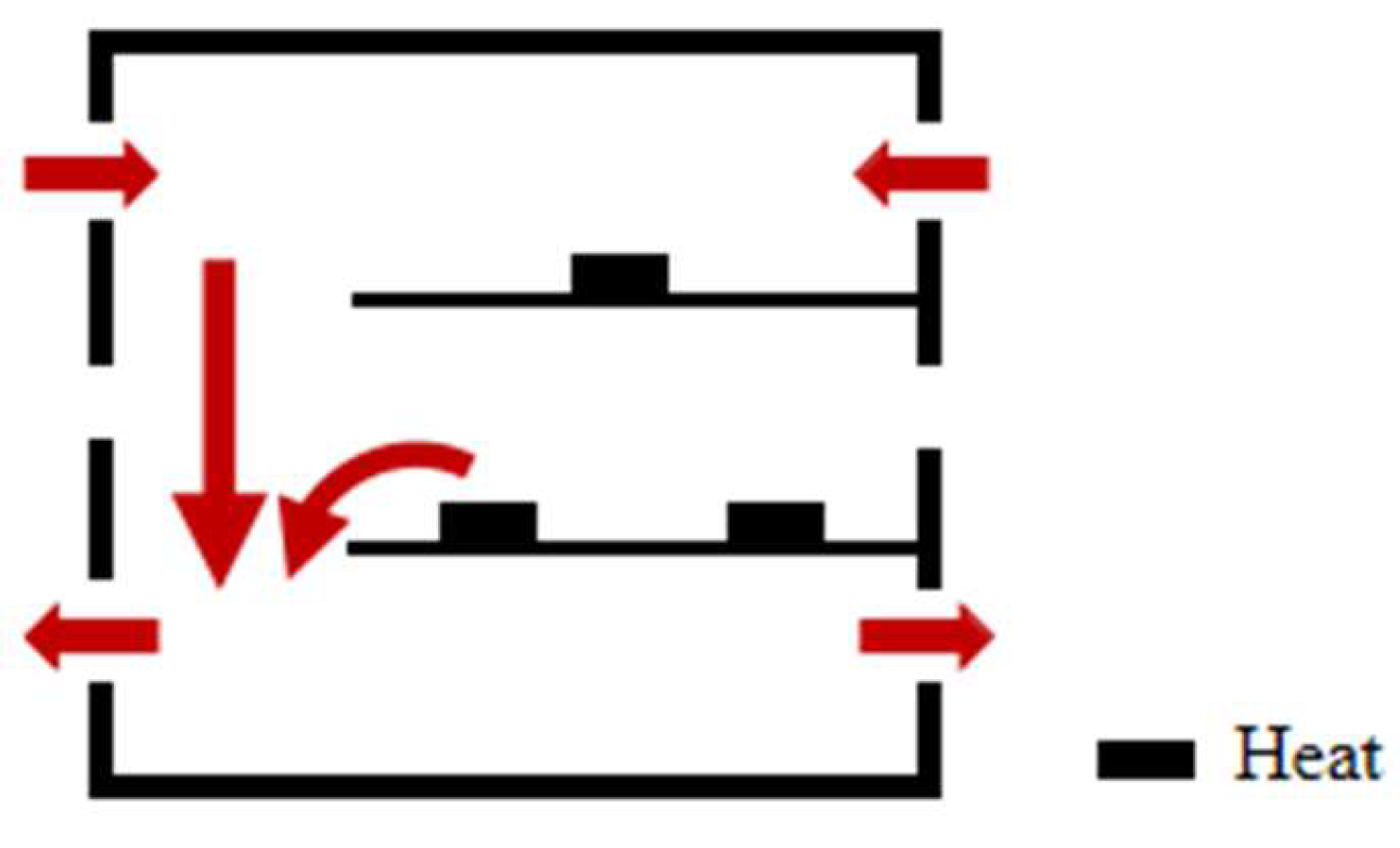
Grs = 0.20 —that is, when a certain intensity of outdoor thermal pressure is applied to the plant—the indoor airflow is mainly influenced by the applied outdoor thermal pressure, generating a flow mode whereby the air flows from the top layer to the bottom layer and the middle-layer air also merges with the overall flow. Thus, flow pattern B (FP-B) is defined as an overall downward pattern, with the intermediate layer being involved, and its diagram is shown in
Figure 12.
When the outdoor air temperature continues to decrease, the outdoor thermal pressure Grashof number (Gri−o) gradually increases, and thermal forcing intensifies progressively. The flow visualization reveals a persistent overall downward flow pattern, with the middle-layer air merging with the flow as thermal forcing intensifies. According to the streamlines in the Y = 9 m section under various working conditions, when the applied outdoor thermal pressure strength is not large, the air entering from the negative X direction through the window on the top floor of the plant flows down to the middle layer along the vertically connected space, and a counterclockwise vortex forms near the heat source, which prevents the air in the middle layer from flowing down along the positive X direction with the overall airflow to the bottom layer to a certain extent. With the continuous increase in outdoor thermal pressure strength, the vortices formed near the heat source in the middle layer decrease continuously. When Gri−o/Grs = 0.40, it can be found that there are basically no vortices at the corresponding position. At the same time, it can be found from the velocity contours that with the increase in the applied outdoor thermal pressure strength, the speed of the outdoor air entering the plant from the top floor continues to increase.
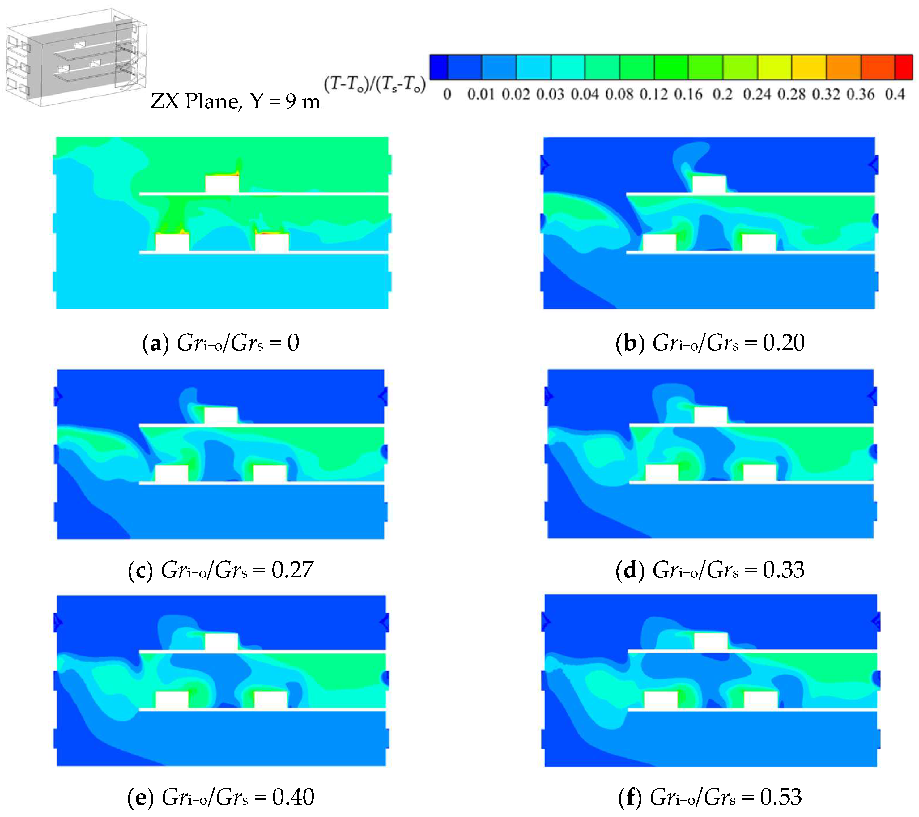
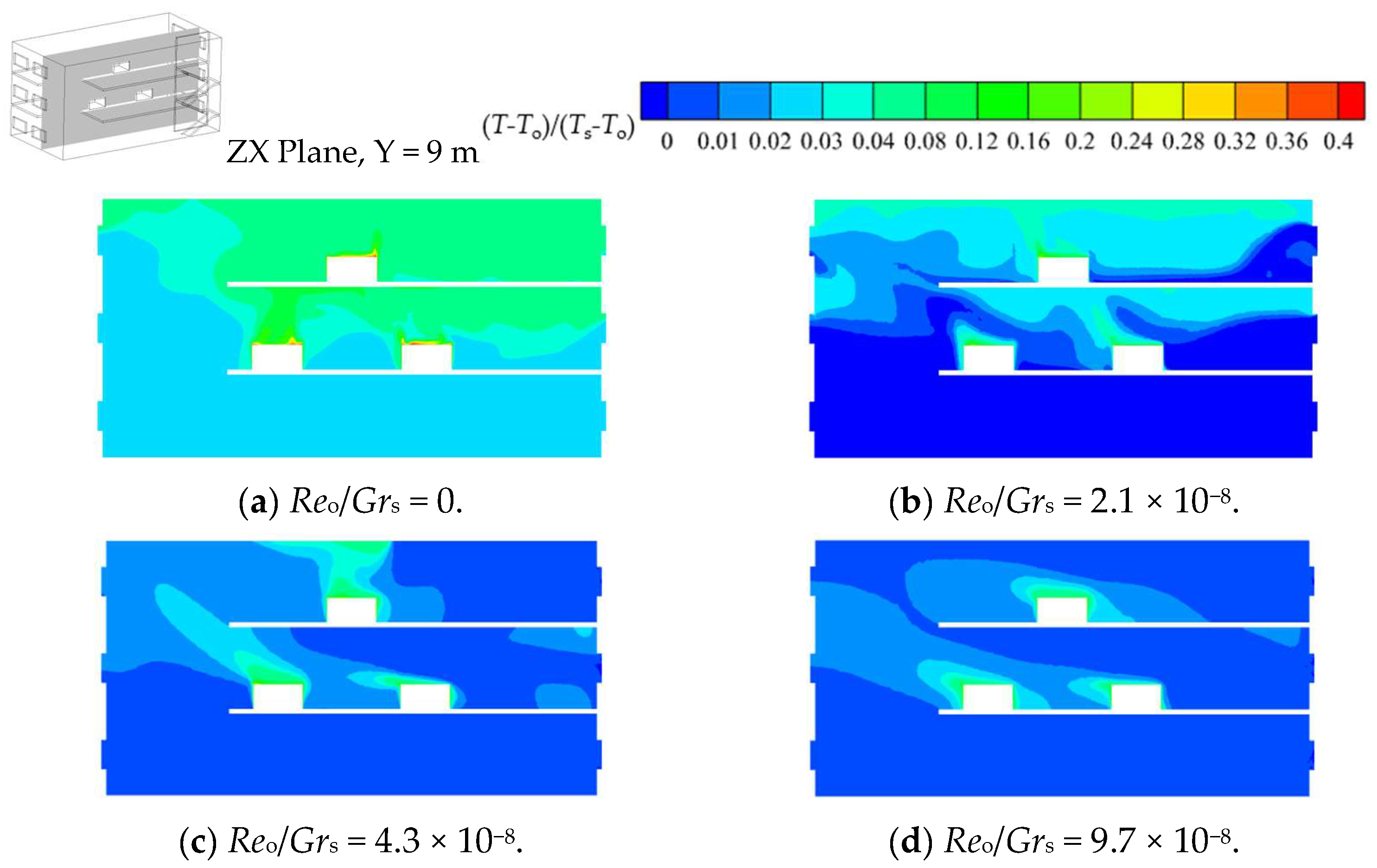
When this type of plant is used for industrial production, the heat emitted by processing equipment drives the indoor airflow while also affecting the thermal environment on all levels of the plant. We next investigated the effect of applying outdoor thermal pressure at different strengths on the thermal environment of each layer of the plant, and
Figure 11 shows the dimensionless temperature contours on the ZX plane at Y = 9 m.
From
Figure 13a, it can be found that when no outdoor heat pressure is applied, the temperature is higher in the working areas on the top and middle floors of the plant. After the fresh outdoor air enters the plant from the windows on both sides of the bottom floor, it flows upward along the vertically connected space to the top floor, where most of it flows out from the side windows, resulting in a lower temperature at the bottom of the structure. The heat on the top and middle floors is thus not dissipated effectively.
When outdoor heat pressure is applied, the temperature of the working area on the top floor of the plant becomes almost the same as that of the fresh outdoor air because the latter enters the plant from the windows on both sides of the top floor and then flows to the bottom floor along the vertically connected space. The temperature of the middle-layer working area is still not effectively dissipated. Because the middle-layer hot airflow also follows the overall airflow to the bottom of the plant, the temperature of the bottom-layer working area is also relatively high.
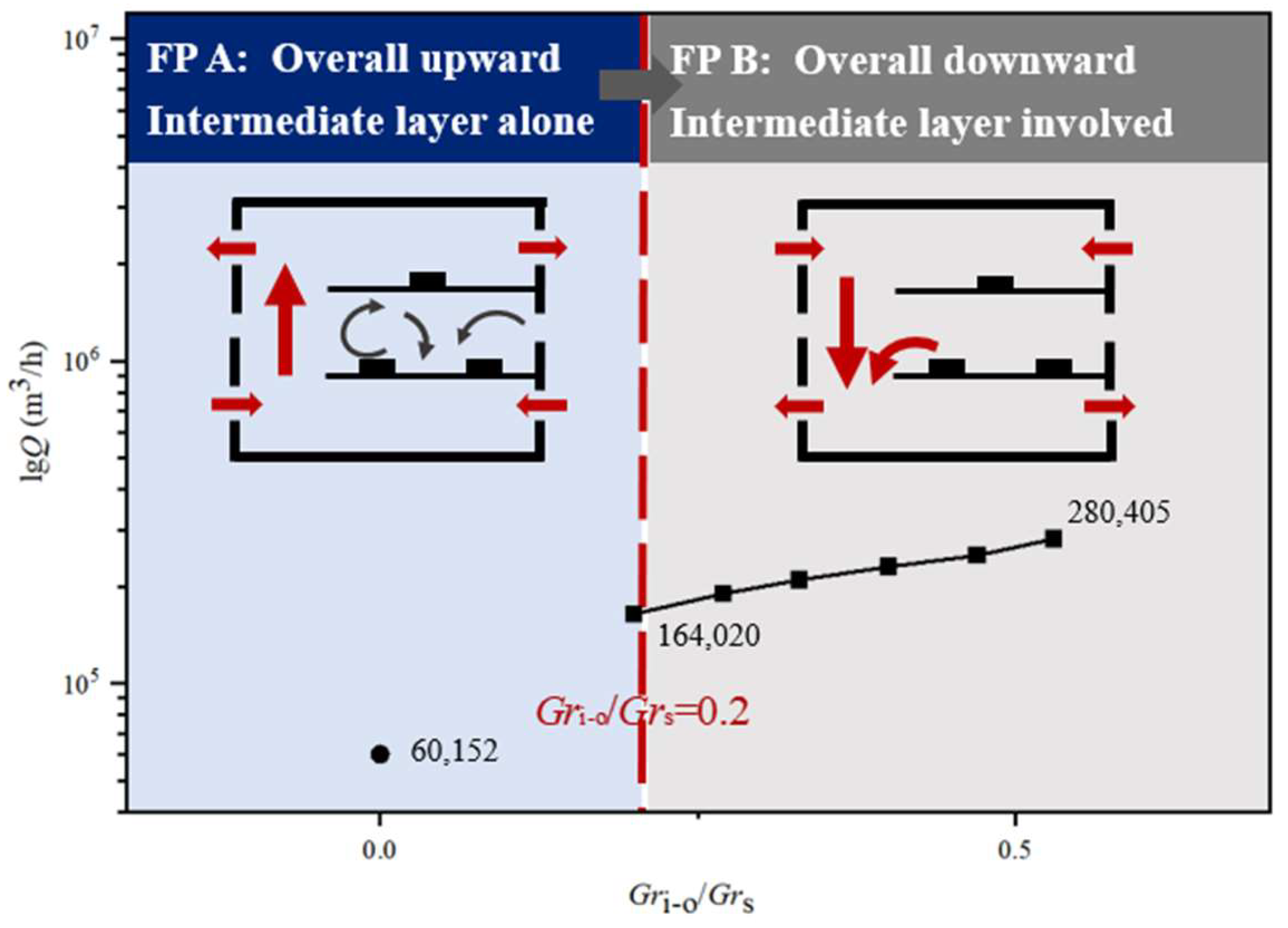
The natural ventilation volume of the plant under various working conditions and outdoor thermal pressure was calculated, and its variation diagram was drawn, as shown in
Figure 14. It can be found that when the flow pattern in the plant changes from the overall upward flow mode where the middle-layer air does not merge with the flow to the overall downward flow mode where the middle-layer air merges with the flow, the natural ventilation volume of the plant increases by about 2.87 times. With the increase in the outdoor thermal pressure, the ventilation volume increases continuously. When
Gri−o/
Grs increases from 0.20 to 0.53, natural ventilation increases by 71%.
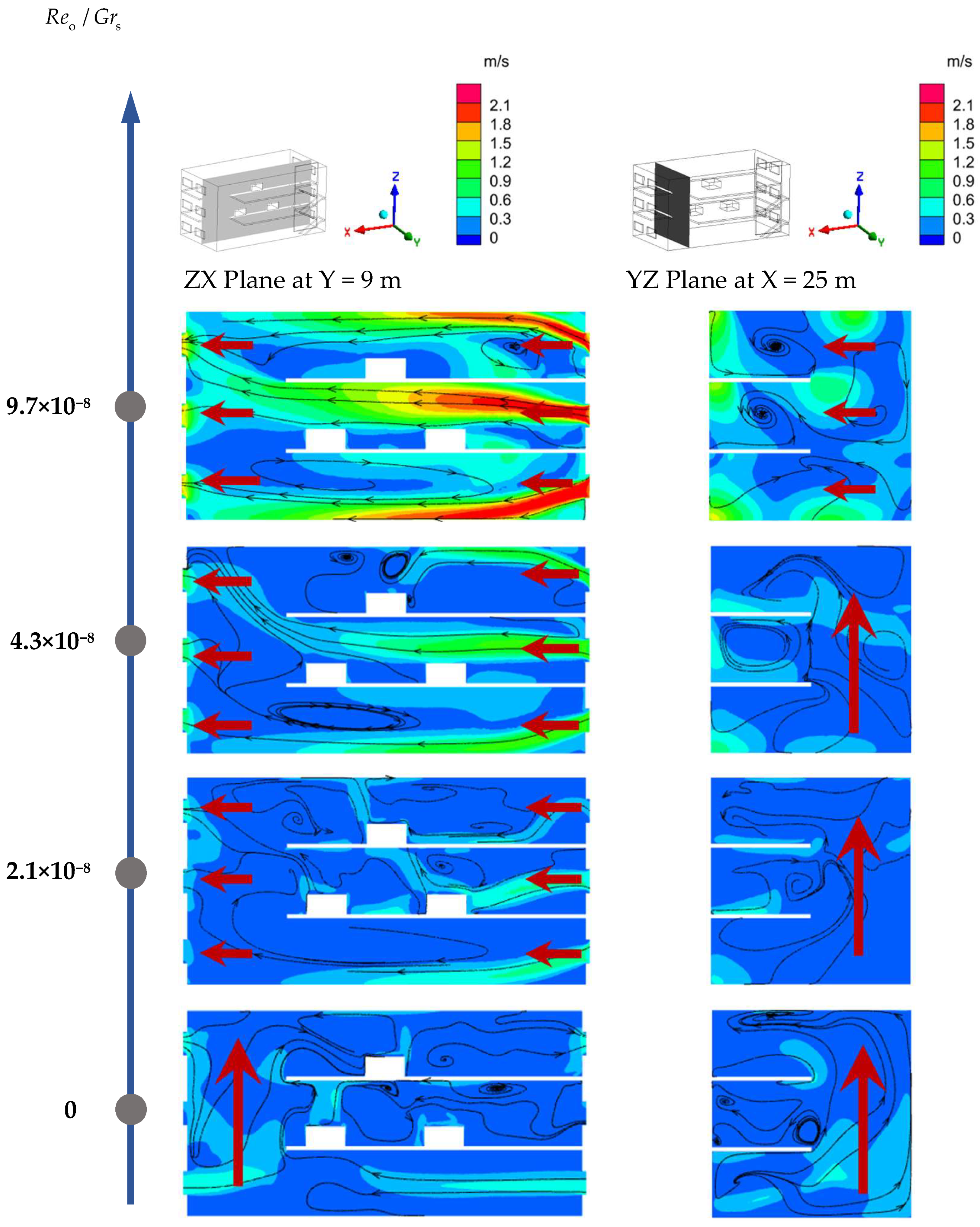
3.3. Effect of Outdoor Wind Pressure on the Airflow in Plant
Figure 15 demonstrates the velocity contours and streamline plots for the ZX cross-section (Y = 9 m) and YZ cross-section (X = 25 m) of the industrial building under in-creasing wind pressure applied to its non-vertically connected structural side. When the effect of outdoor wind pressure is applied, the airflow is jointly driven by the indoor heat source and the outdoor wind pressure. It can be found that when the wind pressure is applied to this side of the plant and the ratio of outdoor natural ventilation Reynolds number to the indoor heat source Grashof number (
Reo/
Grs) increases from 0 to 2.1 × 10
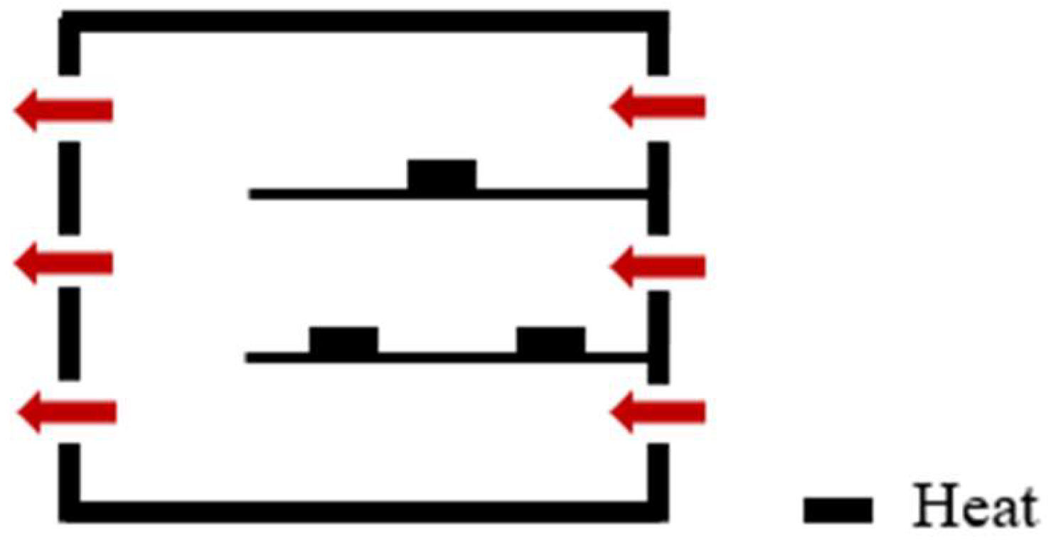
−8, the outdoor wind enters the plant from the windows on the non-vertically connected structure side and then flows out of the plant from the windows on the vertically connected structure side after passing through the working areas on each level. It is worth noting that when the strength of outdoor wind pressure is low, the air, driven by the buoyancy force caused by the heat sources arranged on each floor, is lifted upward to a certain extent when it enters from the side windows of the non-vertically connected structure of the plant. With the increase in outdoor thermal pressure, the lifting amplitude gradually decreases. By observing the YZ cross-section at X = 25 m, it can also be found that when the strength of the applied outdoor wind pressure is low, air still partly flows from the bottom floor to the top floor along the vertically connected space. When
Reo/
Grs increases to 9.7 × 10
−8, straight through flow mainly influenced by outdoor wind pressure is fully formed in the plant. FP-C is defined as a straight through flow, and its diagram is shown in
Figure 16.
We investigated the effect of applying different outdoor wind pressure intensities on the thermal environment of each floor of the plant, and
Figure 17 shows the dimensionless temperature contours on the ZX plane at Y = 9 m. When
Reo/
Grs = 2.1 × 10
−8, i.e., when an out-door wind speed of 1 m/s is applied to the non-vertically connected structure side of the plant, it can be found that the overall indoor thermal environment is greatly improved compared with the case where outdoor wind pressure is not applied. However, as the strength of the applied outdoor wind pressure is still small at this time, horizontal flow has not fully formed in the plant, and the working areas on the middle and top floors still present a large amount of heat that has not been dissipated. With the increase in the strength of the outdoor wind pressure, when
Reo/
Grs = 9.7 × 10
−8, it can be found that the remaining heat can be dispersed by the fresh air flowing from the window of the non-vertically connected side of the plant. The overall thermal environment in the plant is better.
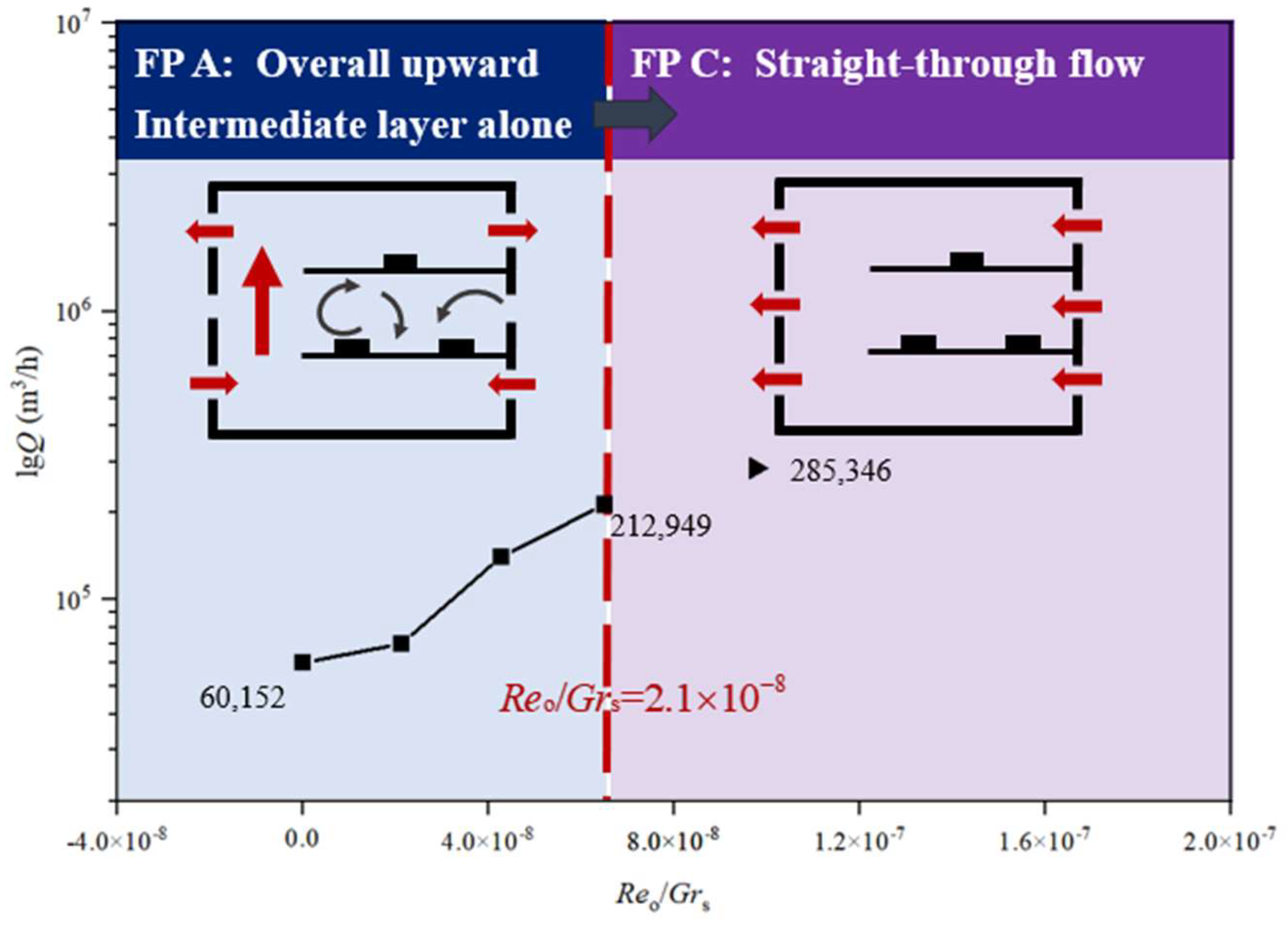
The natural ventilation volume of the plant under different outdoor wind pressure intensities was obtained through calculation, and its variation diagram was drawn, as shown in
Figure 18. It can be found that when the flow pattern in the plant changes from overall upward flow where the middle-layer air does not merge with the flow (FP-A) to straight through flow dominantly influenced by wind pressure (FP-C), the natural ventilation volume of the plant increases. When the ratio of natural ventilation Reynolds number to the indoor heat source Grashof number (
Reo/
Grs) increases from 2.1 × 10
−8 to 9.7 × 10
−8, the natural ventilation volume increases by more than three times.
3.4. Classification of Different Airflow Patterns
In this section, we classify the airflow patterns that can be formed in a multi-layer vertically connected plant under different natural ventilation conditions to clarify the effects of outdoor wind and thermal pressure on airflow within such plants. A classification according to the airflow characteristics of each flow pattern can facilitate the formulation of a more reasonable ventilation optimization scheme for different flow types, allowing for the prediction of the flow pattern that may exist in a plant under other conditions.
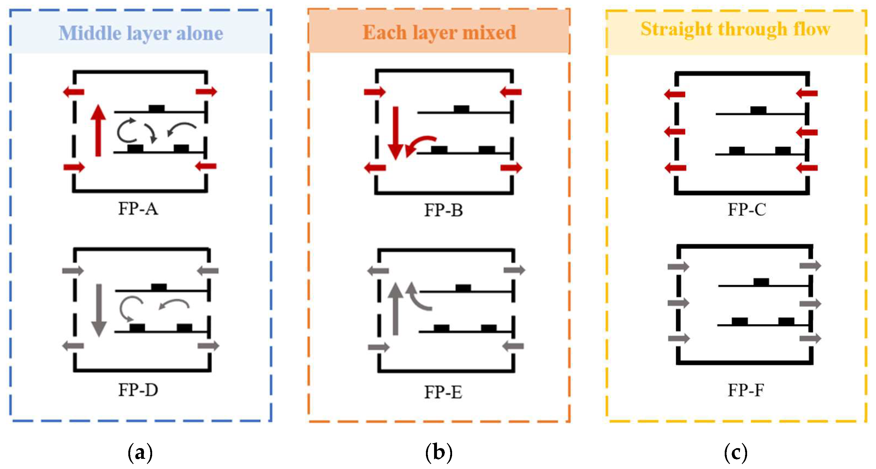
The flow patterns can be divided into three categories: (a) middle layer alone flow, (b) each layer mixed flow and (c) straight-through flow. In the middle layer alone flow, as shown in FP-A in
Figure 19a, when
Gri−o/
Grs = 0 and
Reo/
Grs = 0, air flows from the bottom to the top layer in the plant along the vertically connected space, and the middle-layer air does not merge with the overall flow. In the flow mode of each layer mixed flow, FP-B in
Figure 19b, when
Gri−o/
Grs increases from 0 to 0.2, the airflow gradually changes into flow dominantly influenced by outdoor thermal pressure. The air flows from the top layer to the bottom layer, and the air in the middle layer merges with the overall downward flow. In the straight-through flow, FP-C, as shown in
Figure 19c, occurs when there is outdoor wind pressure on the side of the non-vertically connected structure. When
Reo/
Grs gradually increases from 0 to 9.7 × 10
−8, the air flow fully changes into the flow dominated by outdoor wind pressure. The air flows into the non-vertically connected structure windows of the plant and flows out of the windows on the opposite side.
Moreover, we can predict the airflow patterns that may exist in the plant under other conditions. It is predicted that when outdoor thermal pressure is applied at a certain in-tensity, FP-D, as shown in
Figure 19a, may be formed, a pattern whereby air flows from the top of the plant to the bottom layer, with the middle-layer air not merging with the flow. When fewer heat sources are arranged in the room or their intensity is reduced, FP-E, as shown in
Figure 19b, may be formed, whereby air flows from the bottom layer to the top layer, with the middle-layer air merging with the overall upward flow. If outdoor wind pressure is applied at a certain intensity on the side of the vertically connected structure, it is predicted that FP-F, as shown in
Figure 19c, can be formed, whereby air flows into the plant through the windows on the side of the vertically connected structure and out of the plant through the opposite windows, forming a straight through flow towards the other side.
The above classification summarizes the airflow patterns that can be formed in the considered type of plant under different outdoor environmental conditions. Moreover, the airflow patterns are distinguished into three airflow states, based on which we can not only predict the possible airflow patterns in this type of plant under other conditions but also lay the foundation for the scientific optimization of this type of plant environment.


