Crack Propagation Behavior Modeling of Bonding Interface in Composite Materials Based on Cohesive Zone Method

Abstract

Wood, steel, and concrete constitute the three predominant structural materials employed in contemporary commercial and residential construction. In composite applications, bond interfaces between these materials represent critical structural junctures that frequently exhibit a reduced load-bearing capacity, rendering them susceptible to the initiation of cracks. To elucidate the fracture propagation mechanisms at composite material interfaces, this study implements the cohesive zone method (CZM) to numerically simulate interfacial cracking behavior in two material systems: glued laminated timber (GLT) and reinforced concrete (RC). The adopted CZM framework utilizes a progressive delamination approach through cohesive elements governed by a bilinear traction–separation constitutive law. This methodology enables the simulation of interfacial failure through three distinct fracture modes: mode I (pure normal separation), mode II (pure in-plane shear), and mixed-mode (mode m) failure. Numerical models were developed for GLT beams, RC beams, and RC slab structures to investigate the propagation of interfacial cracks under monotonic loading conditions. The simulation results demonstrate strong agreement with experimental cracking observations in GLT structures, validating the CZM’s efficacy in characterizing both mechanical behavior and crack displacement fields. The model successfully captures transverse tensile failure (mode I) parallel to wood grain, longitudinal shear failure (mode II), and mixed-mode failure (mode m) in GLT specimens. Subsequent application of the CZM to RC structural components revealed a comparable predictive accuracy in simulating the interfacial mechanical response and crack displacement patterns at concrete composite interfaces. These findings collectively substantiate the robustness of the proposed CZM framework in modeling complex fracture phenomena across diverse construction material systems.

1. Introduction

With advancements in modern technology and the enhancement of residents’ living requirements, contemporary structures are evolving towards larger spans and multi-story designs [1,2,3]. Composite materials, owing to their favorable mechanical properties and cost-effectiveness, are becoming the primary construction materials for a multitude of buildings [4,5,6]. Among these, the two most widely used composite materials in industrial or civil construction are glued laminated timber (GLT) and reinforced concrete (RC). A GLT Post and Beam Structure (GTPBS) is favored in timber engineering, primarily due to its commendable seismic resistance [7], and RC members are serving as the major main load-bearing structures in many large-scale projects, e.g., commercial buildings, bridges, tunnels, etc. Within GLT and RC materials, bond interfaces are prevalent and often constitute the weakest links in the structure, making them prone to bond breaking and crack formation [8,9,10,11]. Confronted with complex loading and environmental conditions, such as temperature fluctuations and corrosive actions, these factors can potentially lead to the degradation and cracking of bond interfaces [12], thereby affecting the overall stability of the structure. Consequently, an in-depth investigation into the cracking behavior of composite material cohesive interfaces is of paramount theoretical and practical significance for predicting the durability and safety of structures.

The bond interfaces in GLT and RC structures encompass the complete cohesive region between timber and adhesive materials, as well as the interfacial transition zone between steel reinforcement and concrete. This region plays a pivotal role in GLT and RC structures [13], where an interaction occurs between wood and adhesive materials, or concrete and steel reinforcement, i.e., a bond anchorage effect [14]. This interaction enables the two materials to effectively work in concert, jointly bearing loads and fully utilizing the load-bearing capabilities of the materials. In practice, the bond performance at the bond interface is subjected to several influencing factors. These factors encompass, but are not confined to, load effects, temperature variations, material defects, the type of adhesive used, the bond line thickness achieved, the duration of curing, environmental conditions during bonding and curing processes, etc. [15,16]. The bond strength at the interfaces of GLT and RC structures may degrade, leading to potential slippage and subsequent cracking at these interfaces. Such cracks or minor crushing may propagate longitudinally along the bond interface or develop transversely, exhibiting significant structural damage that adversely affects the overall stability and safety of the structure.

The cohesive zone method (CZM) represents a well-established numerical modeling approach for simulating interfacial failure and fracture propagation in composite material systems. This computational framework introduces a cohesive zone at material interfaces to characterize progressive failure mechanisms. In contrast to abrupt fracture models, the CZM conceptualizes material failure as a gradual degradation process. Extensive research over several decades has systematically validated the CZM’s predictive capability regarding crack initiation and propagation phenomena. Consequently, this methodology has gained widespread adoption in investigating the mechanical behavior of engineered composites, including glued laminated timber (GLT) and reinforced concrete (RC) structures.

2. Theory of the Cohesive Zone Method (CZM)

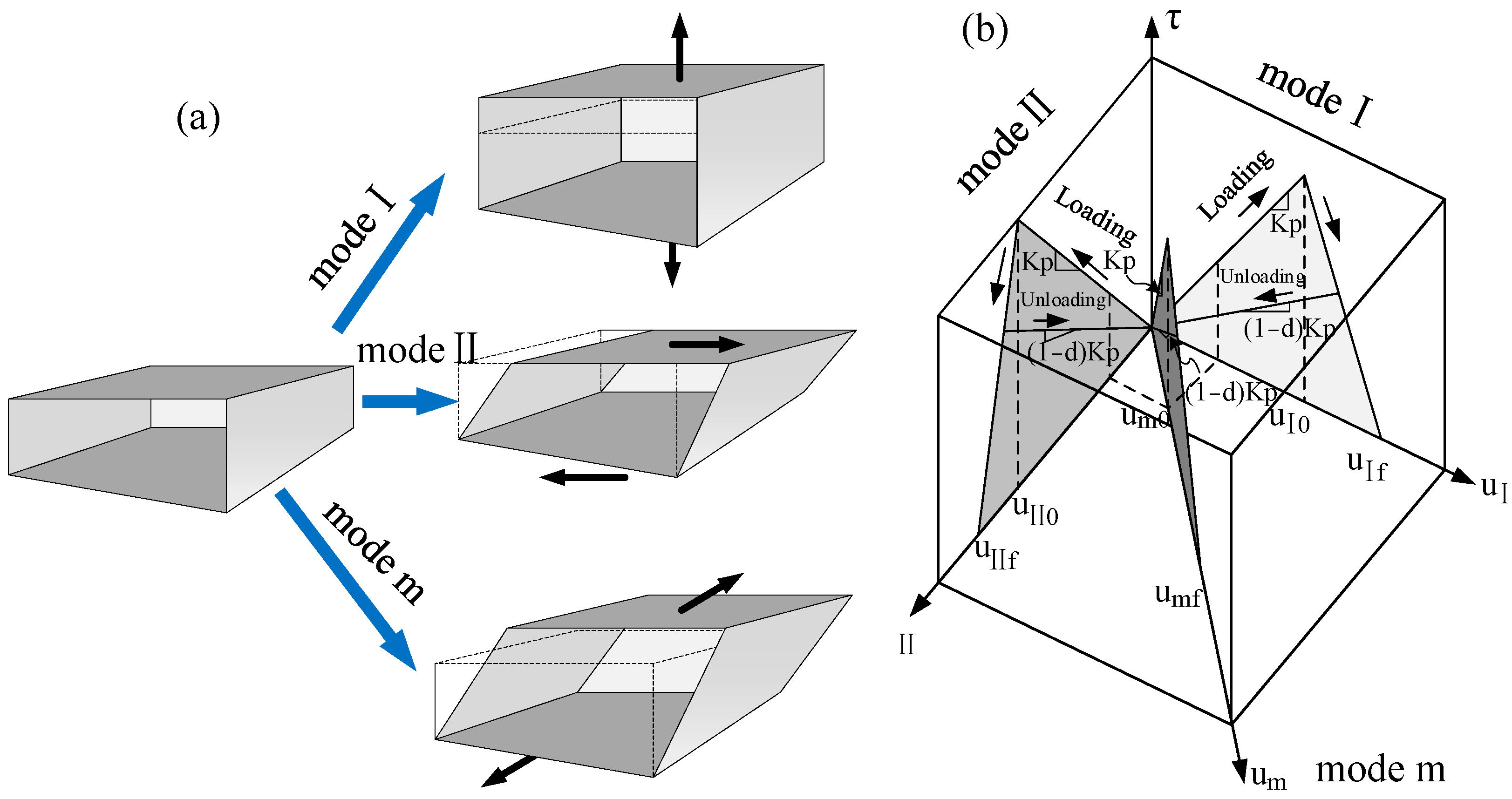
2.1. Numerical Implementation of Debonding Zones for Delamination Modeling in Composite Materials

The computational representation of debonding zones, employed to simulate progressive delamination in composite materials, is conventionally implemented through interfacial elements connecting adjacent plies within composite laminates. These debonding elements serve to numerically characterize the displacement discontinuities induced by delamination’s propagation. Based on their spatial discretization methodology, these interfacial elements are systematically classified into two distinct types: (1) continuum interface elements, which maintain a finite geometric dimension along the interface, and (2) discrete point interface elements, which localize the interfacial behavior at nodal points. Several types of continuous interface elements have been proposed, including zero-thickness planar interface elements that connect solid elements [17,18], planar interface elements with a finite thickness connecting shell elements [19], line interface elements [20,21,22], and a spring interface element for the connection node pair [23]. To predict the initiation and propagation of delamination, an 8-node decohesion element, as illustrated in Figure 1, is employed in the CZM. The element is designed to simulate the interface between sublayers or two bonded components and consists of zero-thickness (t ≈ 0) volume elements. The material response embedded within these elements utilizes the cohesive zone ahead of the crack tip to represent damage, thereby forecasting delamination propagation.

For the constitutive modeling of interface elements for fracture simulations, the accurate numerical representation of interfacial fracture processes fundamentally depends on the appropriate formulation of constitutive equations that establish the relationship between interfacial stress (σ) and separation displacement (δ). Several strain-softening constitutive models have been proposed in the past decades, including the bilinear elastic–perfectly plastic model, the linear elastic with linear softening degradation model, the linear elastic with progressive nonlinear softening model, the linear elastic with exponential softening degradation model, and the Needleman model [25]. All strain-softening models share a characteristic that, after the initiation of damage (δ > δ₀ in Figure 2), the cohesive zone can still transmit loads. For single-loading mode I or II, after the interfacial normal stress or shear stress reaches its respective interlaminar tensile or shear strength, the stiffness gradually diminishes until it reaches zero. The area under the stress–relative displacement curve represents the corresponding fracture energy for each mode (I or II). If using the J-integral (Equation (1)) proposed by Rice [26], it can be demonstrated that, for small cohesive zones, the linear elastic–linear softening (bilinear) model is the most straightforward to implement and the most commonly used model.

$${\int }_0^{{\delta }^F}\sigma (\delta )d\delta =G_c$$

(1)

where G_c is the critical energy release rate for a specific mode, and δ^F is the corresponding separation displacement at failure.

The linear elastic–linear softening (bilinear) model is illustrated in Figure 3a, and Figure 3b displays the material displacement observed during the composite cantilever beam tensile test. The bonding interface at Point 1 in Figure 3b is subjected to a low tensile load in a linear elastic range, and the high initial stiffness K_p (penalty stiffness) closely combines the top and bottom sides of the interface element. In the delamination of a single mode, the stress at Point 2 is equal to the corresponding interlaminar ultimate strength, σ_c, of the material, which represents the beginning of damage. As the reverse load continues to increase after the interface damage accumulates, the stress will be lower than the corresponding interlayer strength, σ_c, of the material at Point 3, and the energy released at this time is equal to the area of the 0–2–3 triangle, as shown in Figure 3a. If unloaded at this time, the stress is assumed to be linear from Point 3 to the origin. Point 4 is the critical value of the energy release rate. For any relative displacement greater than Point 4, the interface does not bear any tensile or shear load (Point 5); that is, at point 4, all available interface fracture energy has been exhausted.

The bilinear interface constitutive response shown in Figure 3 can be realized as follows:

(1) When δ < δ⁰, the constitutive equation is

$$\sigma =K_p\delta$$

(2)

(2) When δ⁰ ≤ δ < δ^F, the constitutive equation is

$$\sigma =(1-D)K_p\delta$$

(3)

(3) When δ ≥ δ^F, all penalty stiffnesses are zero. If crack closure is detected, penetration is prevented only by reapplying the normal stiffness, and the friction effect is ignored.

$$\sigma =0$$

(4)

where D represents the cumulative damage at the interface, which is initially 0 and 1 when the material is completely damaged.

The properties required to define the bilinear interface softening process include the initial stiffness (penalty stiffness), K_P. The accuracy of the analysis depends on the selected penalty stiffness, K_P. A high K_P value can avoid the mutual penetration of the crack surface, but it may lead to numerical problems. Daudeville et al. modeled the interface as a layer of a viscous zone with a small thickness and proposed a penalty stiffness defined as the following [28]:

$$K_p^I={\displaystyle \frac{E_I}{l_i}}$$

(5)

$$K_p^{II}={\displaystyle \frac{2K_{II}}{l_i}}$$

(6)

$$K_p^{III}={\displaystyle \frac{2K_{III}}{l_i}}$$

(7)

where E_I is the elastic modulus of the viscous region, and K_II and K_III are the shear modulus of the viscous region.

After a large number of numerical experiments, Davila et al. found that when the penalty stiffness is 10⁶ N/mm³ for all modes, the convergence problem that may occur in the nonlinear process can be avoided, and the same results are obtained [27]. In the structural application of composite materials, the propagation of delamination is likely to occur under mixed-mode (mode m) loads. Therefore, the general formula of interface elements must deal with the propagation of delamination problem in a mixed mode (mode m). The deformation characteristics and the bilinear material response of three modes are shown in Figure 4a. The mixed-mode softening law can be represented in a single 3D graph, with mode I represented on the τ-δ_I plane and mode II represented on the τ-δ_II plane, as shown in Figure 4b.

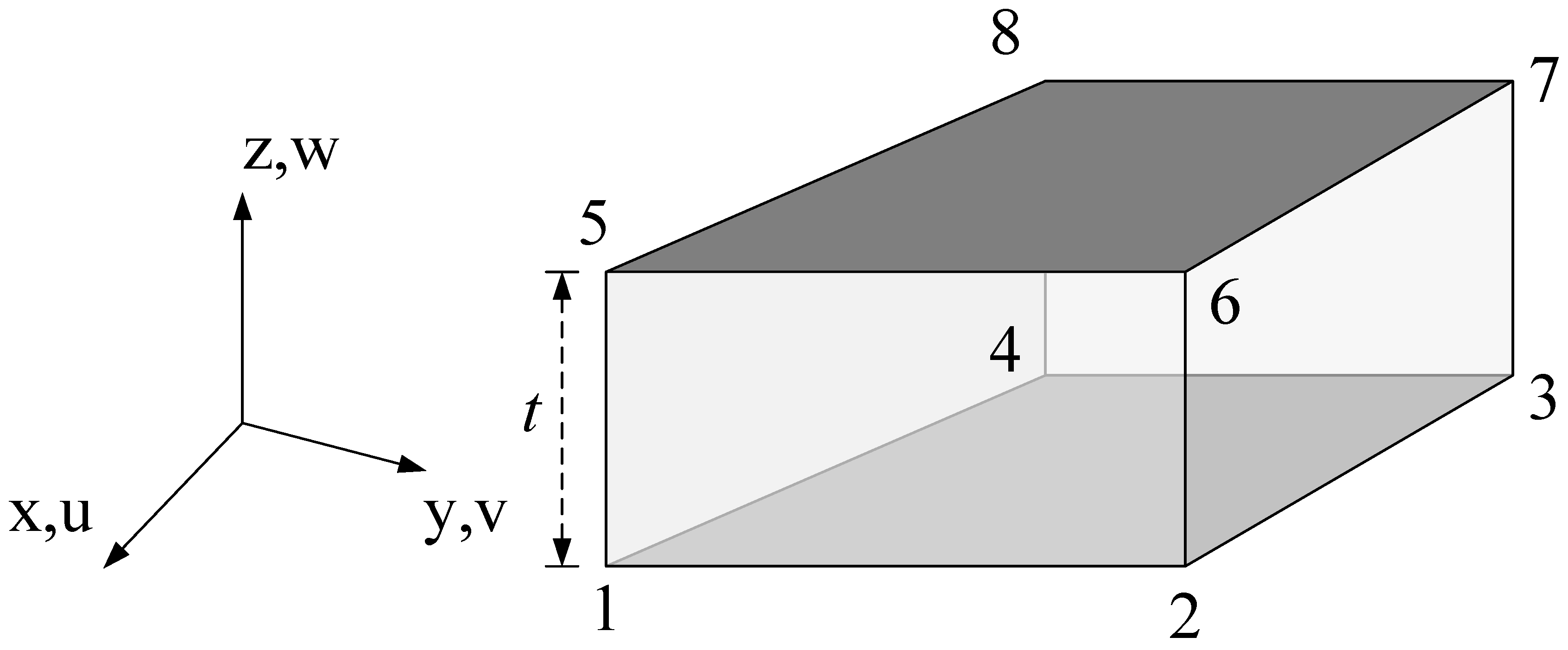
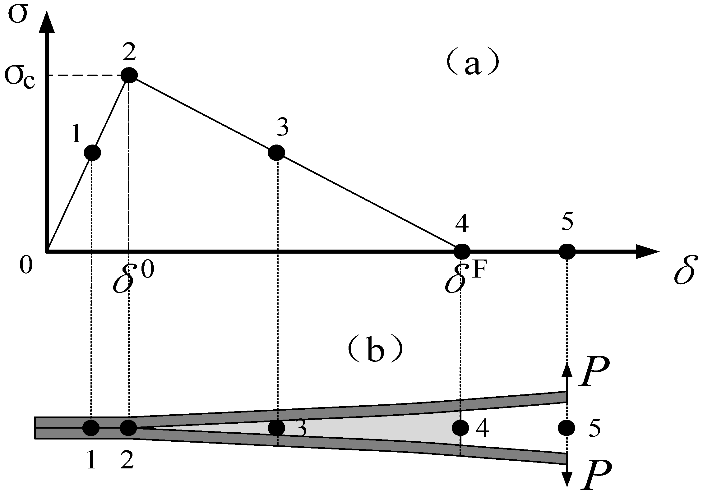
2.2. Geometric Configuration and Constitutive Framework of the Bonding Element in CZM

The constitutive equation in three-dimensional form is

$$\mathit{\sigma }=(\mathit{I}-\mathit{D})\mathit{C}\mathit{\delta } \mathbf{or} \left\{\begin{array}{c}{\sigma }_z\\ {\tau }_{xz}\\ {\tau }_{yz}\end{array}\right\}=(\mathit{I}-\mathit{D})\mathit{C}\left\{\begin{array}{c}{\delta }_z\\ {\delta }_x\\ {\delta }_y\end{array}\right\}$$

(8)

where I is the unit matrix, and C is the undamaged constitutive matrix,

$$\mathit{C}=\left[\begin{array}{ccc}{K}_p^I& 0& 0\\ 0& K_p^{II}& 0\\ 0& 0& K_p^{III}\end{array}\right]$$

(9)

In Equation (8), D is a diagonal linear matrix representing the accumulated damage at the interface,

$$\mathit{D}=\left[\begin{array}{ccc}{d}_I& 0& 0\\ 0& d_{II}& 0\\ 0& 0& d_{III}\end{array}\right]$$

(10)

The d_i term on the diagonal is the damage parameter in different dimensions, which is a nonlinear function of δ_i^max,

$$d_i={\displaystyle \frac{{\delta }_i^F({\delta }_i^{\max }-{\delta }_i^0)}{{\delta }_i^{\max }({\delta }_i^F-{\delta }_i^0)}}$$

(11)

where δ_i^max is the highest separation displacement experienced by the material; δ_i⁰ is the initial displacement of damage shown in Figure 3a; and δ_i^F is the maximum bond displacement shown in Figure 3a.

Under the single-mode I, II, and mixed-mode m loads, it is only necessary to compare the stress components with their respective allowable values to determine whether there is damage at the interface, but it should be emphasized that the onset of interfacial damage (δ > δ₀) does not correspond to the initiation of macroscopic delamination. The traction force of the closed crack is at the maximum value at the beginning of the damage. Under the mixed-mode load, the start of the damage may occur before the corresponding stress components reach their respective allowable values. Here, some simplified assumptions are proposed for the mixed-mode standard. It is assumed that the secondary failure criterion can be used to predict the beginning of the delamination.

$$\sqrt{{\left({\displaystyle \frac{{\sigma }_z}{T}}\right)}^2+{\left({\displaystyle \frac{{\tau }_{xz}}{R}}\right)}^2+{\left({\displaystyle \frac{{\tau }_{yz}}{S}}\right)}^2}=1$$

(12)

where σ_z is the transverse normal tensile stress, and τ_xz and τ_yz are the transverse shear stress. T, R, and S are the tensile strength and shear strength, respectively. Suppose that the shear failure is isotropic, i.e., R = S.

The total tangential displacement, δ_II, is defined as the norm of two orthogonal tangential relative displacements, δ_x and δ_y,

$${\delta }_{\mathrm{II}}=\sqrt{{\delta }_x^2+{\delta }_y^2}$$

(13)

The total mixed-mode interface separation displacement, δ_m, is defined as,

$${\delta }_m=\sqrt{{\delta }_z^2+{\delta }_{II}^2}$$

(14)

where δ_z is the normal separation (mode I) displacement. The same penalty stiffness is used in modes I and II. The interlaminar stress is

$${\sigma }_z=K_p^I{\delta }_z$$

(15)

$${\tau }_{xz}=K_p^{II}{\delta }_x$$

(16)

$${\tau }_{yz}=K_p^{III}{\delta }_y$$

(17)

The elastic limit displacement of a single mode is

$${\delta }_x^0={\displaystyle \frac{T}{K_p^I}}$$

(18)

$${\delta }_y^0={\displaystyle \frac{R}{K_p^{II}}}$$

(19)

$${\delta }_z^0={\displaystyle \frac{S}{K_p^{III}}}$$

(20)

Then, combining Equations (13)–(20), the elastic limit displacement of the mixed mode is obtained.

$${\delta }_m^0={\delta }_I^0{\delta }_{II}^0\sqrt{{\displaystyle \frac{1+{\beta }^2}{({\delta }_{II}^0{)}^2+(\beta {\delta }_I^0{)}^2}}}, \beta ={\displaystyle \frac{{\delta }_{II}}{{\delta }_z}}$$

(21)

The quadratic interaction between the energy release rates defines the total interface fracture point when the interface cannot transmit tensile or shear loads. The quadratic interaction criterion can be expressed as

$$\sqrt{{\left({\displaystyle \frac{G_I}{G_{Ic}}}\right)}^2+{\left({\displaystyle \frac{G_{II}}{G_{IIc}}}\right)}^2}\le 1$$

(22)

where G_i is the energy release rate for each specific mode; G_iC is the fracture energy for each specific mode. When the equation is satisfied only in the case of failure, for the bilinear stress–displacement softening law, the critical energy release rates of mode I and mode II are equal to the area of the triangle in Figure 4b.

$$G_{Ic}={\displaystyle \frac{T{\delta }_I^F}{2}}, G_{IIc}={\displaystyle \frac{S{\delta }_{II}^F}{2}}$$

(23)

The energy released by modes I and II is calculated based on the area of the shaded triangle in Figure 4b, which is

$$G_I=G_{Ic}-{\displaystyle \frac{{\delta }_{\mathrm{I}}^F{\delta }_{\mathrm{I}}^0{K}_p({\delta }_z-{\delta }_{\mathrm{I}}^F)}{2({\delta }_{\mathrm{I}}^0-{\delta }_{\mathrm{I}}^F)}}, G_{II}=G_{IIc}-{\displaystyle \frac{{\delta }_{II}^F{\delta }_{II}^0{K}_p({\delta }_{II}-{\delta }_{II}^F)}{2({\delta }_{II}^0-{\delta }_{II}^F)}}$$

(24)

where δ_I^F and δ_II^F are the plastic limit displacements of mode I and mode II, respectively.

For the displacement-based damage model, there are two different criteria to define, namely the quadratic failure criterion (QFC) [29] and the mixed-mode criterion (B-K criterion) proposed by [30]. This study uses the B-K standard, which is expressed as a function of the fracture toughness of mode I and mode II. The plastic limit displacement of mode m calculated using the B-K standard is

$${{\delta }_m}^F={\displaystyle \frac{2}{K_p{\delta }_{\mathrm{m}}^0}}\left[G_{\mathrm{IC}}+\left(G_{\mathrm{IIC}}-G_{\mathrm{IC}}\right){\left({\displaystyle \frac{{{\delta }_{\mathrm{II}}}^2}{{{\delta }_{\mathrm{I}}}^2+{{\delta }_{\mathrm{II}}}^2}}\right)}^{\eta }\right]$$

(25)

where η is the model parameter.

3. Mechanical Behavior and Failure Mechanisms of Bonding Interface in GLT Structures

In timber structures, GLT members are usually connected by bolts and steel plates. However, due to the complex stress state of the wood around the bolt hole, the joint is prone to split cracks near the bolt hole. Under the action of load, the bolt–steel plate connection joints in GLT beams and columns are subjected to bending moment and shear force at the same time. The bolt-hole wall forms transverse tensile stress due to extrusion, and then transverse splitting failure occurs. The bolt-hole wall produces a plastic zone during the bolt extrusion process, and the bolt produces bending deformation and even shear failure. When subjected to earthquake and the external load is large, the edge pins of the glued laminated timber members are destroyed due to local extrusion, and the bolts at the edge of the members are bent and deformed under the load, so that the glued laminated timber beam–column joints become plastic hinges and cannot continue to bear it. In this chapter, CZM is used to simulate the cracking behavior of GLT.

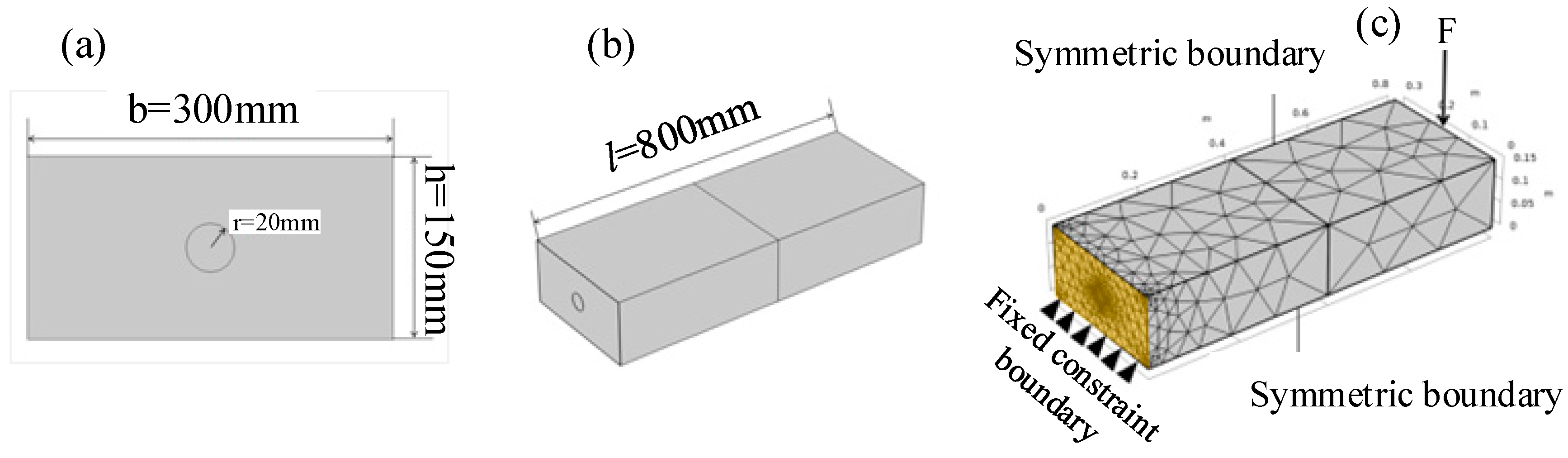
3.1. Mesh Convergence Analysis

In numerical simulations, the refinement level of the mesh significantly influences the accuracy of the computational results. Coarse meshes generally yield a lower precision, whereas excessively fine meshes substantially increase the computational time. To balance this trade-off, a mesh convergence analysis was conducted to determine an optimal mesh configuration.

The computational results under different mesh refinement levels (varying degrees of freedom, DOF) are presented in Figure 5. As shown in Figure 5a, the results obtained with a coarser mesh exhibit pronounced sawtooth-like oscillations, which gradually diminish as the mesh refinement increases. Figure 5b demonstrates that the numerical solution converges with an increasing DOF, and reliable results are achieved when the DOF exceed 30,000.

3.2. Numerical Model and Material Properties of GLT

To make the simulation results comparable with the existing research, the model size is determined according to the test component size referred to by Wang et al. [13]. The beam length is 830 mm, and the section size is 272 × 300 mm. The section size of the column is 130 × 330 mm, and the column length is 1000 mm. The bolt is a hexagonal bolt with a nominal diameter of 20 mm. The Young’s modulus of the bolt is 206 GPa, and the yield strength is 780 MPa. The steel plate is a Q390 steel plate. The thickness is 12 mm. The Young’s modulus is 206 GPa, and the yield strength is 390 MPa. The size of the numerical model and boundary conditions are shown in Figure 6.

The contact element (penalty function) is applied between the beam and column, the glued laminated timber and bolt, and the glued laminated timber interface is simulated by the CZM element. In the test, the GLT specifications were Canadian spruce–pine–cold pine, and the measured water content was in the range of 10–12%. The specific mechanical properties of the specimens were assigned according to the experimental characterization by Wang et al. [13]. The material properties of the steel plate and bolt were selected according to

Table 1. Material properties of the steel plate and bolt referred to by Wang et al. [13].

Materials	Density/(kg/m3)	Young’s Modulus/GPa	Poisson’s Ratio
Steel plate	7870	206	0.29
Bolt	7850	206	0.33

.

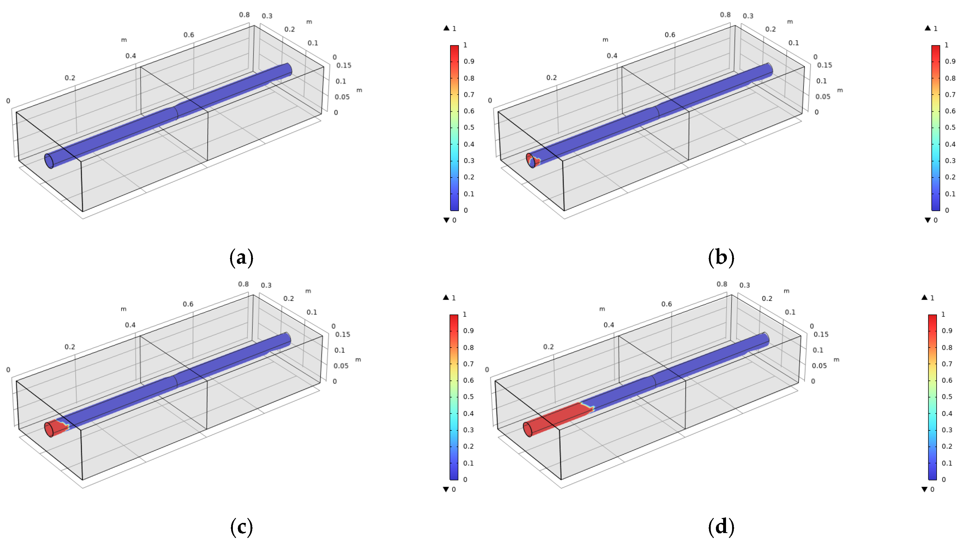
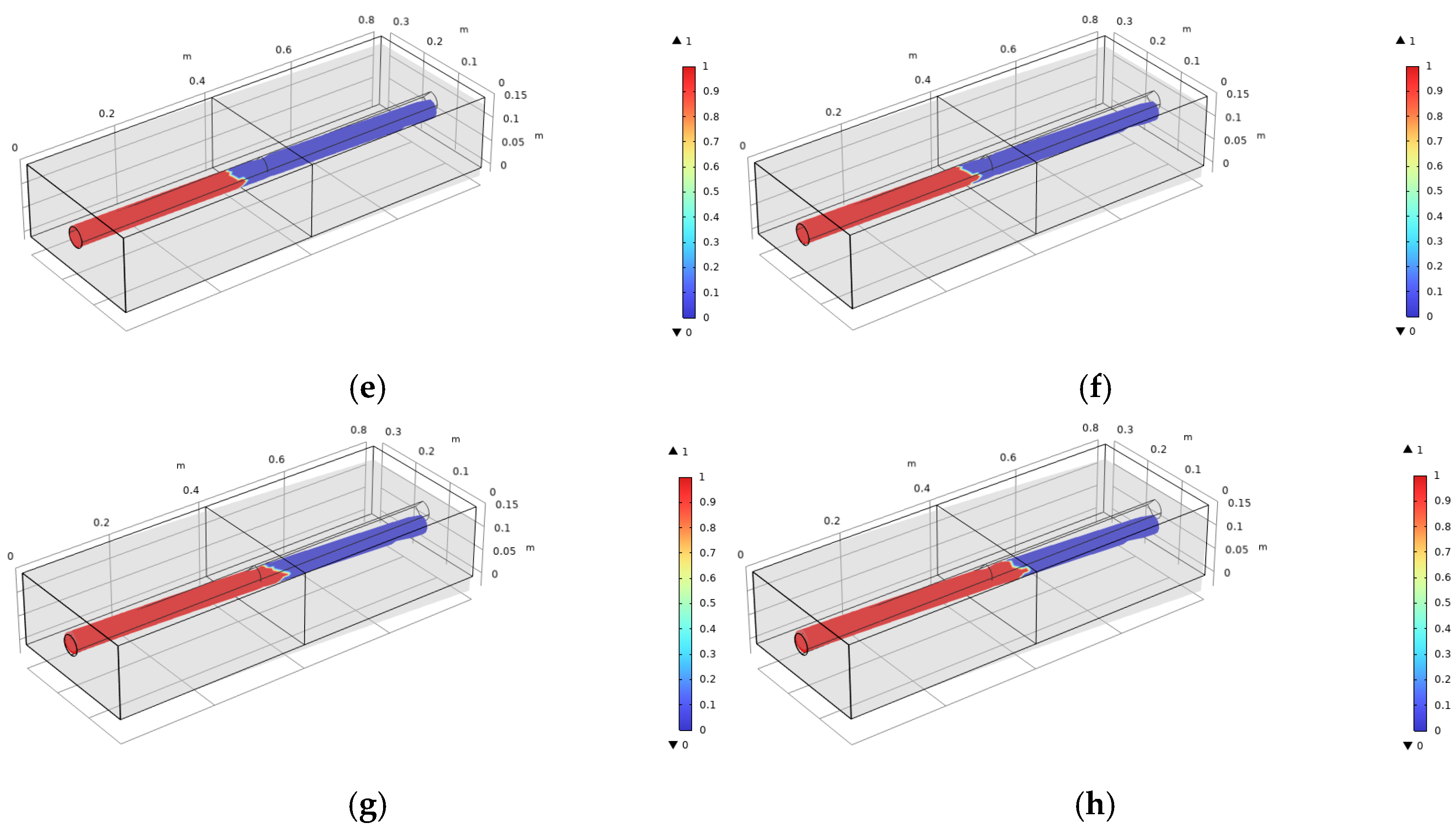
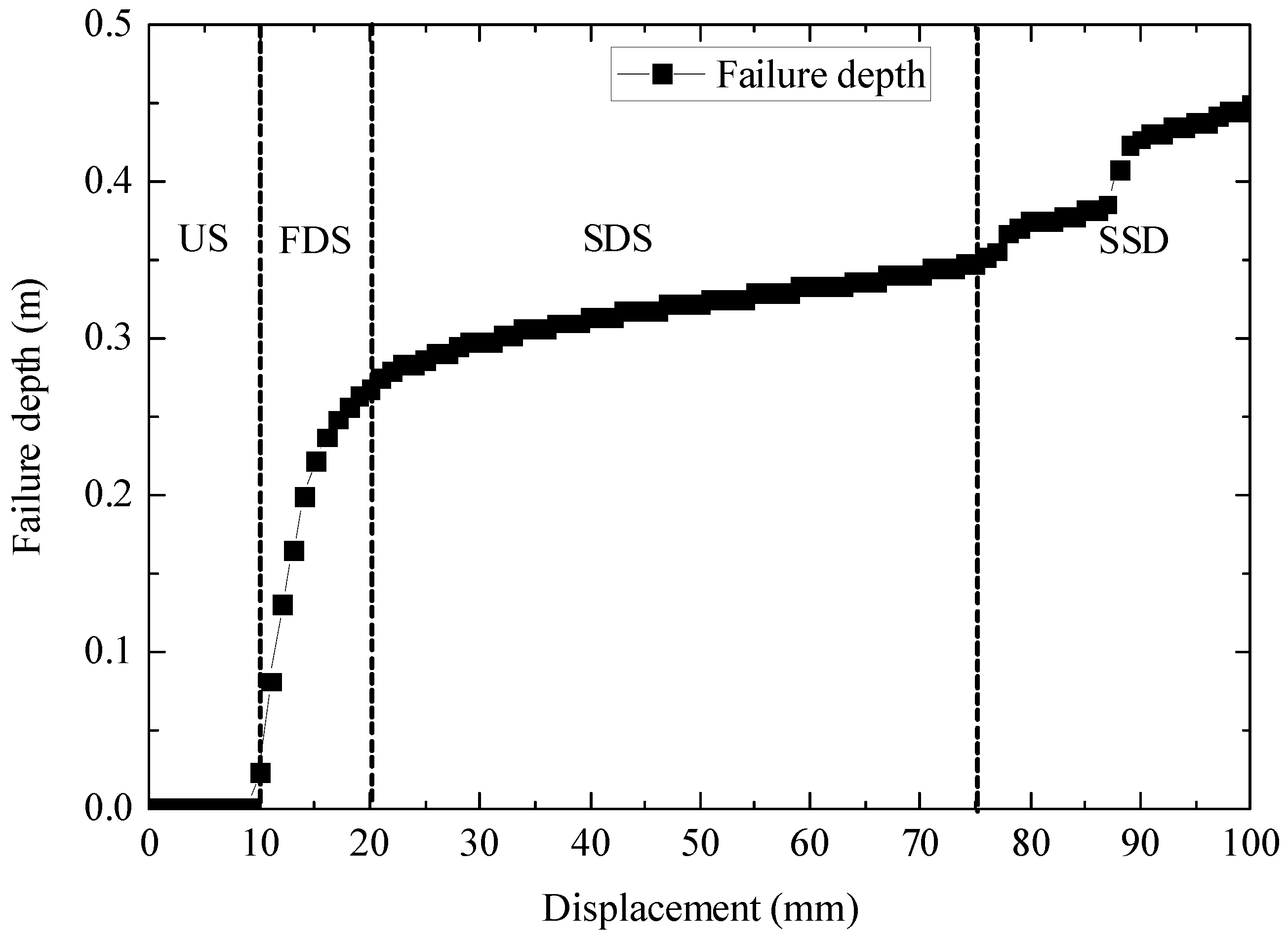
3.3. Numerical Results of GLT Cracking Behavior

The monotonic loading was performed according to the test loading steps of Wang et al. [13], and the loading step was based on the same reference displacement value Δ (Δ = 90 mm). Figure 7 presents the displacement contour plots of the glued laminated timber (GLT) beam–column joints at successive loading increments, illustrating progressive deformation characteristics under applied loading displacement. As evidenced in Figure 7, the displacement response of the glued laminated timber (GLT) beam exhibits progressive development with increasing loading displacement. The deformation of the GLT beam can be divided into five phases. The Initial Loading Phase (0–0.2Δ): when the loading displacement ranges from 0 to 0.2Δ, as the diameter of the bolt is slightly smaller than the diameter of the bolt hole, there is no effective contact between the bolt and the glued laminated timber beam due to the initial gap. Contact Initiation Phase (0.2–0.4Δ): when the loading displacement reaches 0.2~0.4Δ, the corner of the lower end of the glued laminated timber beam–column joint is in contact with the glued laminated timber column and squeezed. Elastic–Plastic Deformation Phase (0.4–1.2Δ): when the loading displacement reaches 0.4~1.2Δ, the GLT beam, bolts, and steel plate are subjected to deformation together, but cracks have not yet occurred. Failure Initiation Phase (1.2-1.6Δ): when the loading displacement reaches 1.2~1.6Δ, transverse splitting failure occurs at the upper part of the glued laminated timber beam along the two rows of bolts along the direction of the grain, which is consistent with the test results of Wang et al. [13]. Crack Propagation Phase (>1.6Δ): when the loading displacement is greater than 1.6Δ, the crack continues to expand until it is completely destroyed or stopped the loading.

By comparing the numerical results (Figure 7h) with the existing experimental results obtained by Wang et al. [13], it is proved that the finite element model based on CZM theory successfully simulates the cracking behavior of a glued laminated timber beam caused by the extrusion around the bolt hole at the position of glued laminated timber beam–column joint under a monotonic loading mode; however, the simulated values of the yielding moment, maximum moment, and failure moment are all lower than the experimental values as shown in

Table 2. Comparison of measured and simulated moment resistances.

Moment (kN∙m)	Yielding Moment	Maximum Moment	Failure Moment
Experiment data from Wang et al. [13]	33.9	38.4	27.9
Simulation data	30.1	30.1	26.6

, which may be due to differences in the loading’s application between the numerical simulation and the experimental test. For details, refer to the experimental setup in Wang et al. [13] and Figure 6b in this study. Figure 8 shows the simulated loading force vs. displacement of GLT beam–column joints under monotonic loading. The results show that when the loading displacement of the glued laminated timber beam reached 1.47~1.6∆ (∆ = 90 mm), the loading force experienced the first steep drop while the loading displacement was still increasing. The main reason is that the upper part of the glued laminated timber beam cracked along the two rows of bolts along the direction of the grain, which is consistent with the experimental results that the failure of the glued laminated timber beam occurs at about 1.5~1.6∆, and which proves that the simulation results have a good accuracy in their calculations. Accordingly, the CZM used in this paper has a good applicability in simulating the mechanical behavior and cracking displacement of glued laminated timber beam–column joints with embedded steel plate–bolt connections. When the loading displacement of the glued laminated timber beam reached 2.24~2.5∆ (∆ = 90 mm), the loading force experienced the second steep drop while the loading displacement was still increasing, meaning that the lower part of the glued laminated timber beam was split along the two rows of bolts along the direction of the grain.

4. Mechanical Behavior and Failure Mechanisms of Bonding Interface in RC Beam

4.1. Numerical Model and Material Properties of RC Beam

The geometric size of the reinforced concrete beam model is shown in Figure 9. The beam length, l, is 800 mm. The section size is b × h = 300 × 150 mm. The radius of the steel bar is r = 20 mm, and this is placed in the middle of the concrete beam. The material properties of the concrete and the steel bar are utilized according to

Table 3. Material properties of concrete and steel bar.

Materials	Density/(kg/m3)	Young’s Modulus/GPa	Poisson’s Ratio
Concrete	2350	28	0.2
Steel bar	7870	206	0.29

. The material properties of the CZM interface are listed in

Table 4. Material properties of the bond interface referred to by Liu [31].

Properties	Value
Normal tensile strength, T	2.31 MPa
Shear strength, R = S	11.4 MPa
Penalty stiffness, Kp	106 N/mm3
Tension critical energy release rate, GIc	93.8 J/m2
Shear critical energy release rate, GIIc	3363.6 J/m2
B-K standard index, η	2.284

.

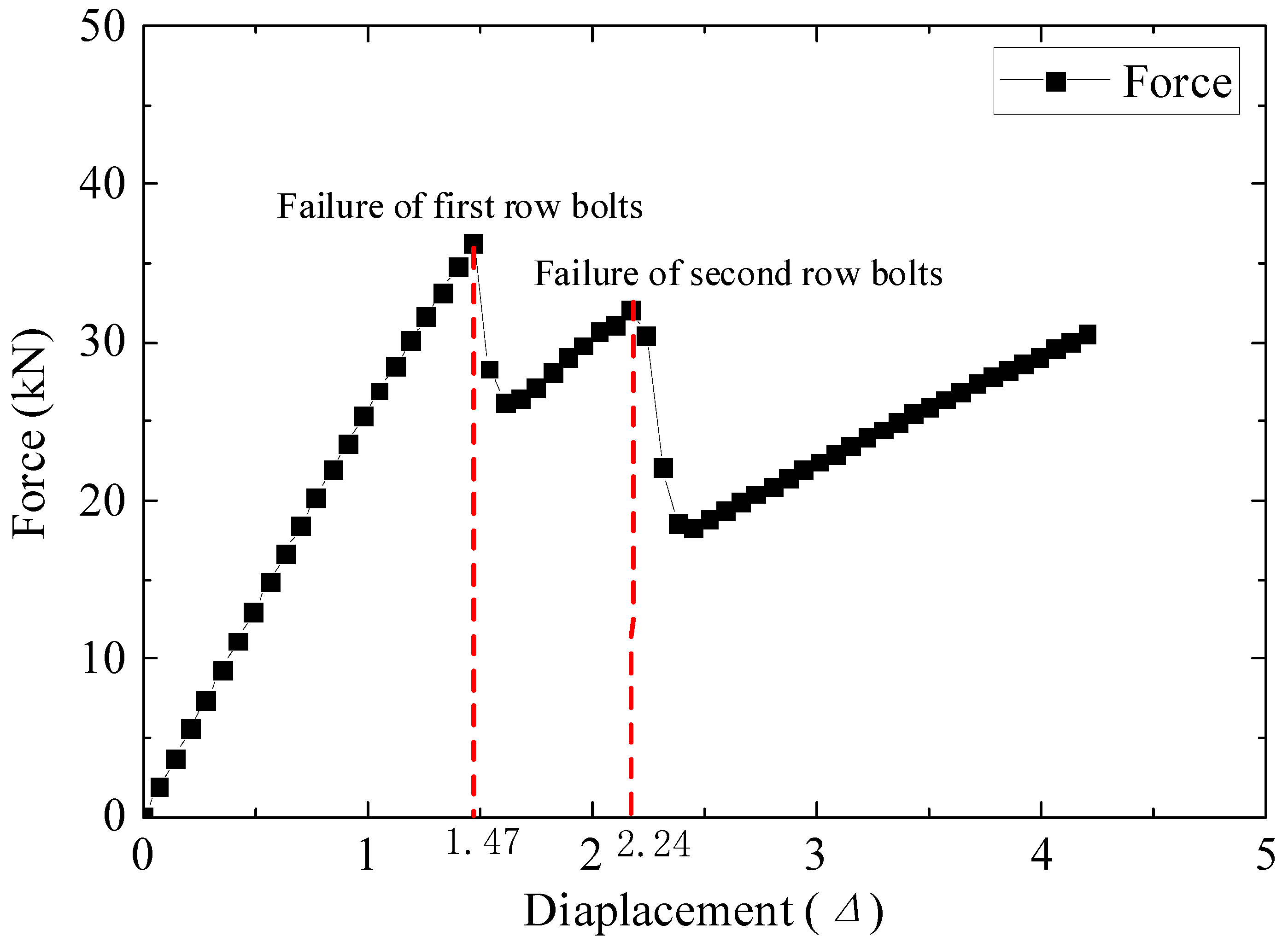
4.2. Numerical Results of RC Beam Cracking Behavior

The progressive failure behavior at the bonding interface was analyzed using an incremental loading scheme with a constant displacement step of 1.0 mm. Figure 10 presents the corresponding failure contour plots at successive loading stages, to illustrate the characteristics of the damage’s evolution, the progressive development of interfacial failure zones, the spatial distribution of damage indicators, and crack propagation patterns, as well as the numerical implementation of a displacement-controlled loading protocol, contour visualization of failure criteria satisfaction, and quantitative representation of the damage’s extent.

The interfacial failure is governed by the following criterion: when the maximum separation displacement (δ_max) exceeds the critical limit displacement (δ_m^F), complete interfacial failure occurs, resulting in fracture and subsequent delamination. To quantitatively characterize this failure process, a reference line is established along the bonding interface. Progressive failure propagation is tracked through loading increments, and the failure depth is measured relative to the fixed constraint boundary. The relationship between the applied loading displacement and the corresponding progression in failure depth is presented in Figure 11. From Figure 10 and Figure 11, it can be observed that the failure depth curve illustrates the nonlinear advancement of damage. The failure depth curve can be divided into four stages according to its slope. Undamaged Stage (US): When the loading displacement is 0~8 mm, the maximum separation displacement δ_max of the interface does not reach the limit displacement δ_m^F, and the interface is intact without damage. Fast Developing Stage (FDS): When the loading displacement reaches 9 mm, the interface breaks for the first time. After that, when the displacement continues to increase to 20 mm, the failure depth increases rapidly to 0.25 m. Slow Developmental Stage (SDS): When the loading displacement increases from 20 mm to approximately 75 mm, the failure depth reaches 0.35 m, and the failure occurs slowly and evenly. Second Stage of Development (SSD): When the loading displacement is greater than 75 mm, the failure occurs relatively violently in this area and changes rapidly, as well as several step-like jumps appearing. When the loading displacement reaches 100 mm, the maximum failure depth is 0.449 m.

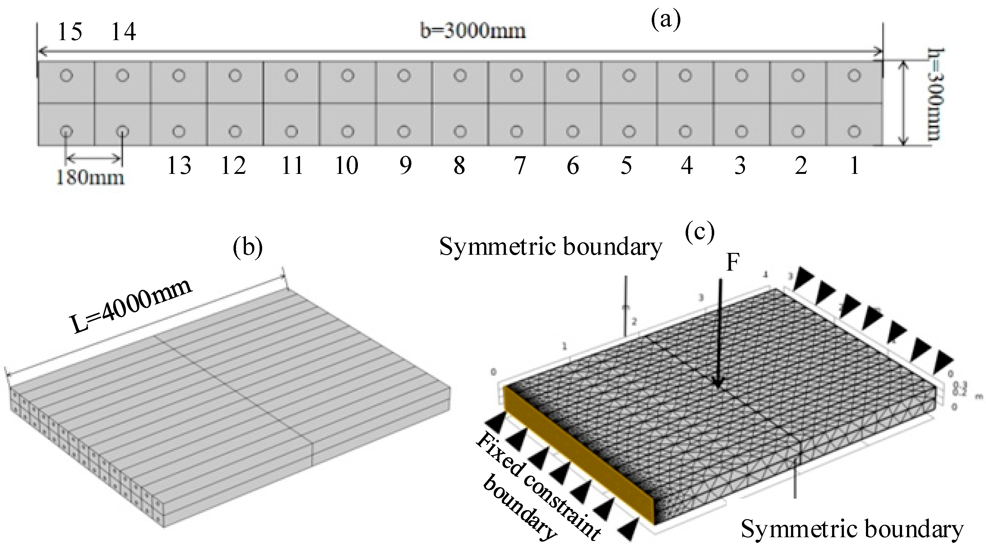
5. Mechanical Behavior and Failure Mechanisms of Bonding Interface in RC Slab

5.1. Numerical Model and Material Properties of RC Slab

Based on the numerical model of the RC beam, an RC slab with a cross-section size of b × h = 3000 × 300 mm, a span of l = 4000 mm, a steel bar radius of r = 20 mm, and a spacing of a = 180 mm was established to observe and analyze the state of the reinforced concrete bonding interface under monotonic loading. The geometric size is shown in Figure 12a,b. The boundary conditions such as fixed constraints and roller supports were set on the reinforced concrete slab model. The finite element model with mesh is shown in Figure 12c.

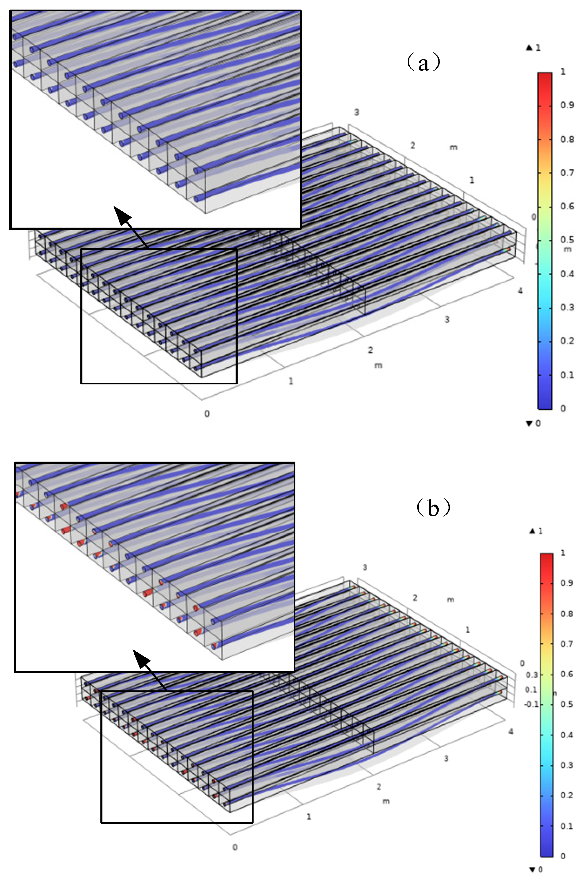
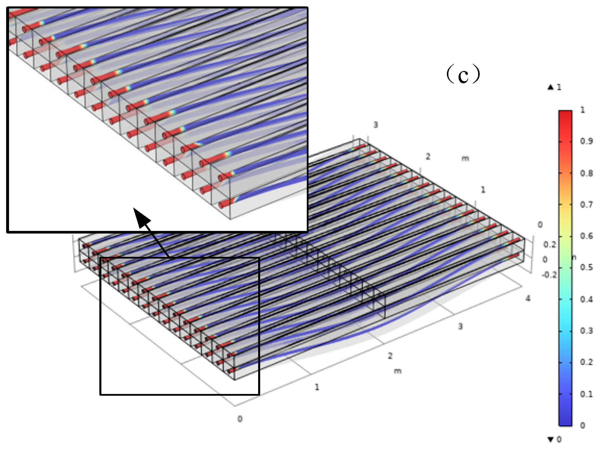
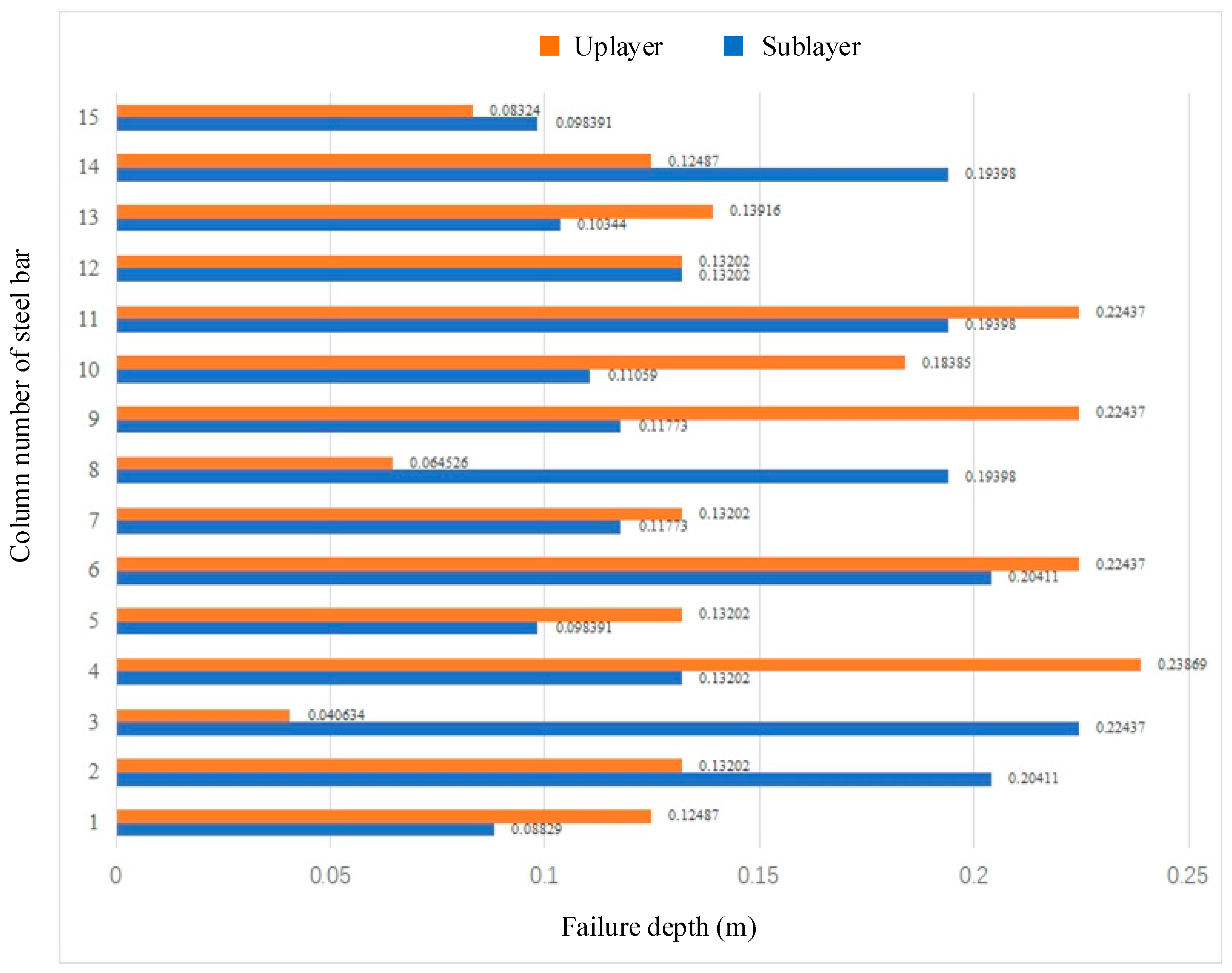
5.2. Numerical Results of RC Slab Cracking Behavior

The model was subjected to monotonic loading up to a displacement of 100 mm. Figure 13a shows the corresponding failure contour plot of the reinforced concrete bonding interface when the loading displacement is 60 mm. When the loading displacement reaches 80 mm, the corresponding failure contour plot of the model is shown in Figure 13b. When the loading displacement reaches 100 mm, the corresponding failure contour plot of the reinforced concrete bonding interface is shown in Figure 13c. From Figure 13, it can be seen that when the loading displacement reaches 60 mm, the damage has not yet occurred (Figure 13a), while when the loading displacement reaches 80 mm, some of the ends of the steel bars are cracked (Figure 13b). Finally, when the loading displacement reaches 100 mm, almost all the ends of the steel bars are cracked and extended to a certain depth in the RC slab (Figure 13c). To quantitatively evaluate the relationship between loading and bonding interface failure, the calculated force curve vs. loading displacement is plotted in Figure 14. It can be observed from Figure 14 that the force–displacement curve exhibits typical quasi-brittle failure characteristics. In the initial stage of loading, the force increases linearly with the increase in loading displacement. However, when the loading displacement reaches 84 mm, a platform appears in the force–displacement curve. When the loading displacement is between 84 mm and 86 mm, the displacement continues to increase, but the required force remains unchanged. When the loading displacement is greater than 86 mm, the force continues to increase linearly with the increase in the loading displacement.

To discuss the spatial difference between the vertical and horizontal effects of the loading, the steel bar is divided into upper and lower layers, numbered 1~15 from left to right as shown in Figure 12a. The maximum failure depths of all the bonding interfaces are summarized in Figure 15 when the loading displacement reaches 100 mm. From Figure 13 and Figure 15, it can be observed that the bond interface of the reinforced concrete slab cracks from the fixed end on both sides to the middle under the action of the load. In all the failed bonding interfaces, the failure depth of the sublayer steel bar at the third steel bar layer is the largest, reaching 224.37 mm; the damage depth at the first steel bar layer is the smallest, which is 88.29 mm. The failure depth of the fourth steel bar layer of the upper layer steel bar is the largest, reaching 238.69 mm; the failure depth at the third steel bar layer is the smallest, which is 40.634 mm. In general, the degree of damage of the middle reinforced concrete bonding interface is greater than that of the left and right ends, indicating that the interfacial damage exhibits non-uniform distribution patterns, and the middle sections demonstrate more severe damage than the edge regions. The lower reinforcement layer shows a greater variability in damage, and the failure depth differentials suggest stress concentration effects.

6. Conclusions and Discussions

This paper adopts a progressive debonding simulation method based on an eight-node debonding element for the numerical simulation, which further verifies the effectiveness of the CZM in predicting the cracking of the bonding interface and supplements the shortcomings of previous research on the evolution of the damage of the bonding interface, which mainly depends on experimental data.

Subsequently, the CZM is used to simulate the cracking behavior of the bonding interface in GLT beams, RC beams, and RC slab structures to investigate interfacial crack propagation under monotonic loading conditions. The numerical results exhibit strong concordance with experimental crack propagation observations in GLT specimens, thereby confirming the model’s capability to accurately characterize both mechanical response and crack displacement fields. Moreover, the CZM overcomes the inherent limitations of conventional finite element methods in simulating material fracturing, particularly in cases involving adhesive interface failure induced by large deformations in GLT components. The model further demonstrates a robust applicability in analyzing the mechanical behavior and crack displacement of GLT beam–column joints with embedded steel plate–bolt connections.

Additionally, the CZM effectively captures the nonlinear progression of damage in RC bonding interfaces. The analysis identifies four distinct stages in the development of failure depth: the Undamaged Stage (US), Rapid Propagation Stage (RPS), Stabilized Development Stage (SDS), and Secondary Development Stage (SDS). The results also reveal that the CZM can accurately represent both the spatial heterogeneity of interfacial damage distribution and stress concentration effects, as evidenced by variations in failure depth.

While this study provides significant insights into the modeling of the crack propagation behavior of the bonding interface in composite materials based on the CZM, certain limitations warrant acknowledgment. The loading methodology and parameter selection may not be entirely generalizable to more complex loading scenarios or diverse structural configurations. Subsequent research should focus on refining the CZM through (1) enhanced parameter calibration under combined loading condition, and (2) improved accuracy in the characterization of material properties. Notably, the current numerical simulations do not fully account for the orthotropic stiffness properties of glued laminated timber (specifically, the distinction between tensile and shear stiffness), nor do they incorporate monotonic cyclic loading simulations or comprehensive experimental validation. Moreover, whether the bilinear traction–separation law adopted in this study can fully simulate the complete range of interfacial failure modes remains an open question. The implementation of nonlinear debonding processes within the cohesive zone model (CZM) framework still requires further discussion, which would necessitate redefining the material’s constitutive curve based on experimental data or theoretical formulations. While this study does not account for time-/environment-dependent material properties (e.g., the inherent anisotropy of GLT, moisture-dependent behavior, or brittle-to-ductile transitions in reinforced concrete), we emphasize that the finite element method (FEM) has the potential capability of modeling such phenomena. Under such scenarios, the cohesive zone model (CZM) parameters (tensile/shear strength, fracture energy) must transition from constants to spatially and temporally varying functions, dependent on moisture content, equivalent plastic strain, and the accumulation of damage, as well as fiber orientation (for timber) or steel–concrete bond degradation.

Furthermore, this study applies a uniform interface property for the entire steel–concrete bond region. In reality, the bond-slip behavior is highly nonlinear and localized around cracks. Therefore, incorporating a bond-slip law or variable interface strength/stiffness should be considered in the subsequent research to better replicate experimental observations. Moreover, structural failure is often induced not by monotonic loading but by cyclic loading, such as seismic actions. Under cyclic degradation mechanisms, the calibration of the CZM parameters requires in-depth investigation, particularly fracture energy and damage evolution. Special attention should be paid to the underlying mechanism whereby localized material imperfections or property gradients may significantly influence fracture behavior. As demonstrated by He et al. [32], mechanical properties vary across thicknesses, while casting defects can lead to significant material inhomogeneity. Masoumi et al. [33] found that pit size significantly affected stress intensity and highlights the importance of the material’s processing and microstructural orientation in determining mechanical properties. In those cases, a damage model is able to achieve regularized softening responses with a localizing gradient enhancement corresponding to the development of macroscopic cracks, to resolve the numerical spurious effects induced by the conventional gradient enhancement [34]. Another limitation of this study is the exclusion of self-weight effects in the fracture mechanics framework. As highlighted by Mercuri et al. [35], neglecting gravitational loads may not be justified for large-scale structures, particularly when dead load significantly contributes to fractures’ initiation and propagation. Future research should address this aspect to improve the model’s accuracy. These factors collectively contribute to the complexity of fracture behavior under cyclic loading conditions, and more aspects should be prioritized in future studies to strengthen the model’s predictive capability.

References

1. Schlopschnat, C.; Pérez, M.G.; Zechmeister, C.; Estrada, R.D.; Kannenberg, F.; Rinderspacher, K.; Knippers, J.; Menges, A. Co-design of fibrous walls for multi-story buildings. J. Clean. Prod. 2023, 235, 235–248. [Google Scholar]
2. Wang, Y.; Li, G.Q.; Zhu, S. Collapse modes and mechanisms of planar multi-story large-span steel frames under fire. J. Build. Eng. 2024, 94, 109924. [Google Scholar] [CrossRef]
3. Malladi, B.P.; Venkateshwaran, A.; Nayaka, R.R. Design and economic implications of using steel fibers in elevated slabs of multi-story buildings. Struct. Concrete 2025, 26, 162–178. [Google Scholar] [CrossRef]
4. Rajak, D.K.; Pagar, D.D.; Kumar, R.; Pruncu, C.I. Recent progress of reinforcement materials: A comprehensive overview of composite materials. J. Mater. Res. Technol. 2019, 8, 6354–6374. [Google Scholar] [CrossRef]
5. Zhang, Y.; Yang, Z.; Xie, T.; Yang, J. Flexural behaviour and cost effectiveness of layered UHPC-NC composite beams. Eng. Struct. 2022, 273, 115060. [Google Scholar] [CrossRef]
6. Jonnala, S.N.; Gogoi, D.; Devi, S.; Kumar, M.; Kumar, C. A comprehensive study of building materials and bricks for residential construction. Constr. Build. Mater. 2024, 425, 135931. [Google Scholar] [CrossRef]
7. Cao, J.; Du, J.; Fan, Q.; Yang, J.; Bao, C.; Liu, Y. Reinforcement for earthquake-damaged glued-laminated timber knee-braced frames with self-tapping screws and CFRP fabric. Eng. Struct. 2024, 306, 117787. [Google Scholar] [CrossRef]
8. Palieraki, V.; Vintzileou, E.; Silva, J.F. Behavior of RC interfaces subjected to shear: State-of-the art review. Constr. Build. Mater. 2021, 306, 124855. [Google Scholar] [CrossRef]
9. Bader, T.K.; Ormarsson, S. Modeling the mechanical behavior of wood materials and timber structures. In Springer Handbook of Wood Science and Technology; Springer: Cham, Switzerland, 2023; pp. 507–568. [Google Scholar]
10. Kallioras, S.; Bournas, D.; Smiroldo, F.; Giongo, I.; Piazza, M.; Molina, F.J. Cross-laminated timber for seismic retrofitting of RC buildings: Substructured pseudodynamic tests on a full-scale prototype. Earthq. Eng. Struct. Dyn. 2024, 53, 4354–4378. [Google Scholar] [CrossRef]
11. Gao, Z.; Gong, M.; Mohammadi, M.; Li, L. In-situ characteristic elastic properties of bond-lines in laminated engineered wood products using microscopic digital image correlation. Int. J. Adhes. Adhes. 2024, 132, 103715. [Google Scholar] [CrossRef]
12. Kytka, T.; Gašparík, M.; Sahula, L.; Karami, E.; Teterin, D.; Das, S.; Kvietková, M.S. Bending characteristics of glued laminated timber depending on the alternating effects of freezing and heating. Constr. Build. Mater. 2022, 350, 128916. [Google Scholar] [CrossRef]
13. Wang, M.; Song, X.; Gu, X.; Zhang, Y.; Luo, L. Rotational behavior of bolted beam-to-column connections with locally cross-laminated glulam. J. Struct. Eng. 2015, 141, 04014121. [Google Scholar] [CrossRef]
14. Ling, Z.; Zhang, H.; Mu, Q.; Xiang, Z.; Zhang, L.; Zheng, W. Shear performance of assembled shear connectors for timber–concrete composite beams. Constr. Build. Mater. 2022, 329, 127158. [Google Scholar] [CrossRef]
15. Hänsel, A.; Sandak, J.; Sandak, A.; Mai, J.; Niemz, P. Selected previous findings on the factors influencing the gluing quality of solid wood products in timber construction and possible developments: A review. Wood Mater. Sci. Eng. 2022, 17, 230–241. [Google Scholar] [CrossRef]
16. Subhani, M.; Lui, H.Y. Effect of Primer and Fibre Orientation on Softwood–Hardwood Bonding. J. Compos. Sci. 2024, 8, 192. [Google Scholar] [CrossRef]
17. De Moura, M.; Gonçalves, J.P.M.; Marques, A.T. Modeling compression failure after low velocity impact on laminated composites using interface elements. J. Compos. Mater. 1997, 31, 1462–1479. [Google Scholar] [CrossRef]
18. Gonçalves, J.P.M.; De Moura, M.; De Castro, P.M.S.T. Interface element including point-to-surface constraints for three-dimensional problems with damage propagation. Eng. Comput. 2000, 17, 28–47. [Google Scholar] [CrossRef]
19. Reedy, E.D., Jr.; Mello, F.J.; Guess, T.R. Modeling the initiation and growth of delaminations in composite structures. J. Compos. Mater. 1997, 31, 812–831. [Google Scholar] [CrossRef]
20. Petrossian, Z.; Wisnom, M.R. Prediction of delamination initiation and growth from discontinuous plies using interface elements. Compos. Part A Appl. Sci. Manuf. 1998, 29, 503–515. [Google Scholar] [CrossRef]
21. Mi, Y.; Crisfield, M.A.; Davies, G.A.O. Progressive delamination using interface elements. J. Compos. Mater. 1998, 32, 1246–1272. [Google Scholar] [CrossRef]
22. Chen, M.; Crisfield, M.; Kinloch, A.J.; Busso, E.P.; Matthews, F.L.; Qiu, Y. Predicting progressive delamination of composite material specimens via interface elements. Mech. Compos. Mater. Struct. 1999, 6, 301–317. [Google Scholar] [CrossRef]
23. Schellekens, J.C.J.; De Borst, R. On the numerical integration of interface elements. Int. J. Numer. Methods Eng. 1993, 36, 43–66. [Google Scholar] [CrossRef]
24. Camanho, P.P.; Davila, C.G.; De Moura, M.F. Numerical simulation of mixed-mode progressive delamination in composite materials. J. Compos. Mater. 2003, 37, 1415–1438. [Google Scholar] [CrossRef]
25. Needleman, A. A continuum model for void nucleation by inclusion debonding. J. Appl. Mech. 1987, 54, 525–531. [Google Scholar] [CrossRef]
26. Rice, J.R. A path independent integral and the approximate analysis of strain concentration by notches and cracks. J. Appl. Mech. 1968, 35, 379–386. [Google Scholar] [CrossRef]
27. Davila, C.; Camanho, P.; de Moura, M. Mixed-mode decohesion elements for analyses of progressive delamination. In Proceedings of the 19th AIAA Applied Aerodynamics Conference, AIAA, Anaheim, CA, USA, 11–14 June 2001; p. 1486. [Google Scholar]
28. Daudeville, L.; Allix, O.; Ladeveze, P. Delamination analysis by damage mechanics: Some applications. Compos. Eng. 1995, 5, 17–24. [Google Scholar] [CrossRef]
29. Cui, W.; Wisnom, M.R.; Jones, M. A comparison of failure criteria to predict delamination of unidirectional glass/epoxy specimens waisted through the thickness. Composites 1992, 23, 158–166. [Google Scholar] [CrossRef]
30. Benzeggagh, M.L.; Kenane, M. Measurement of mixed-mode delamination fracture toughness of unidirectional glass/epoxy composites with mixed-mode bending apparatus. Compos. Sci. Technol. 1996, 56, 439–449. [Google Scholar] [CrossRef]
31. Liu, Y. Perpendicular to Grain Fracture of Curved Glulam Beams-Experiment and Numerical Modelling. Master’s Thesis, Harbin University of Technology, Harbin, China, 2015. [Google Scholar]
32. He, X.; Yam, M.C.; Zhou, Z.; Zayed, T.; Ke, K. Inhomogeneity in mechanical properties of ductile iron pipes: A comprehensive analysis. Eng. Fail. Anal. 2024, 163, 108459. [Google Scholar] [CrossRef]
33. Masoumi, M.; Loureiro, R.C.; Mohtadi-Bonab, M.A.; Béreš, M.; de Abreu, H.F. Analysis of crystallographic orientation and crack behavior in armor wire with spheroidized pearlite: Simulation and modeling with linear elastic fracture mechanics. Eng. Fail. Anal. 2024, 159, 108126. [Google Scholar] [CrossRef]
34. Zhang, Y.; Xu, Y.; Wang, Y.; Poh, L.H. A simple implementation of localizing gradient damage model in Abaqus. Int. J. Damage Mech. 2022, 31, 1562–1591. [Google Scholar] [CrossRef]
35. Mercuri, M.; Pathirage, M.; Gregori, A.; Cusatis, G. Influence of self-weight on size effect of quasi-brittle materials: Generalized analytical formulation and application to the failure of irregular masonry arches. Int. J. Fract. 2024, 246, 117–144. [Google Scholar] [CrossRef]
Figure 1. Eight-node element utilized in the CZM, t ≈ 0 (adopted from Camanho et al. [24]).
Buildings 15 01717 g001
Figure 2. Constitutive models of strain softening (adopted from Davila et al. [27]).
Buildings 15 01717 g002
Figure 3. Linear elastic–linear softening (bilinear) model (adopted from Davila et al. [27]): (a) constitutive models; and (b) material displacement observed during the composite cantilever beam tensile test.
Buildings 15 01717 g003
Figure 4. Deformation characteristics and bilinear material response of three modes: (a) deformation characteristics of three modes; and (b) bilinear material response of three modes.
Buildings 15 01717 g004
Figure 5. Grid convergence test: (a) simulation results under different grid accuracies, (b) convergence of simulation results.
Buildings 15 01717 g005
Figure 6. Size of numerical model referred to by Wang et al. [13]. (a) Size of numerical model; and (b) boundary conditions with mesh.
Buildings 15 01717 g006
Figure 7. The displacement of GLT beam–column joints under monotonic loading (m), when the (a) loading displacement is 0; (b) loading displacement is 0.2Δ; (c) loading displacement is 0.4Δ; (d) loading displacement is 0.8Δ; (e) loading displacement is 1.2Δ; (f) loading displacement is 1.6Δ; (g) loading displacement is 2.0Δ; (h) loading displacement is 2.4Δ.
Buildings 15 01717 g007
Figure 8. Loading force vs. displacement of GLT beam–column joints under monotonic loading.
Buildings 15 01717 g008
Figure 9. Geometric size of RC beam: (a) cross-section, (b) oblique view, and (c) boundary conditions with mesh.
Buildings 15 01717 g009
Figure 10. Failure diagram of bonding interface of RC beam when the loading displacement is (a) 1 mm, (b) 9 mm, (c) 10 mm, (d) 13 mm, (e) 50 mm, (f) 70 mm, (g) 90 mm, and (h) 100 mm.
Buildings 15 01717 g010aBuildings 15 01717 g010b
Figure 11. Failure depth curve vs. loading displacement of RC beam.
Buildings 15 01717 g011
Figure 12. Geometric size and boundary conditions of the RC slab: (a) section size, (b) oblique view, and (c) boundary conditions with mesh.
Buildings 15 01717 g012
Figure 13. Failure depth of bonding interface of RC slab: (a) loading displacement is 60 mm, (b) loading displacement is 80 mm, and (c) loading displacement is 100 mm.
Buildings 15 01717 g013aBuildings 15 01717 g013b
Figure 14. Force curve vs. loading displacement of RC slab.
Buildings 15 01717 g014
Figure 15. Failure depth of each steel bond interface (loading displacement is 100 mm).
Buildings 15 01717 g015