Analysis of Airflow Dynamics and Instability in Closed Spaces Ventilated by Opposed Jets Using Large Eddy Simulations

Abstract

This study quantitatively analyzes the effects of various ventilation parameters on airflow stability in confined spaces ventilated by opposed jets, a common configuration in high-density settings. Using large eddy simulations (LES), we evaluate how changes in supply velocity, airflow configuration, enclosure geometry, and thermal gradients influence airflow dynamics. Findings show that higher supply velocities, up to 1.92 m/s, lead to a measurable increase in oscillation period (from 7.7 s to 11.3 s) and reduce small-scale flow disturbances. The free jet configuration exhibits higher oscillation amplitude and a more disordered structure compared to the attached jet, resulting in uneven airflow distribution. Aspect ratio has a pronounced effect, with increased ratios extending oscillation periods from 10.6 s to 18.1 s and intensifying turbulence. Thermal gradients, with floor temperatures rising from 15 °C to 35 °C, and the oscillation period are increased, further dispersing airflow and reducing stability. Phase space reconstruction and power spectral analysis provide quantitative benchmarks for oscillation frequencies and patterns, correlating velocity time series with airflow structural changes. The findings from this study can serve as a foundation for future research on thermal comfort and air quality management in enclosed environments.

1. Introduction

Respiratory infectious diseases such as influenza, severe acute respiratory syndrome (SARS), and coronavirus disease (COVID-19) have been threatening public health in the past two decades [1,2]. Relevant studies have shown that the virus is mainly spread through respiratory droplets and aerosols in closed spaces where humans live [3,4]. The transmission and distribution patterns of droplets and aerosols in enclosed indoor spaces are intricately determined by indoor airflow distribution and airflow field structure. Consequently, there has been a growing emphasis on the research of indoor airflow distribution and airflow field structure in relation to human habitation in enclosed spaces [5,6,7]. Enclosed indoor spaces primarily encompass residences, workplaces, and transportation vehicles, among others [8]. Airflow distribution and airflow field within these confined areas are fundamental prerequisites for ensuring the safety, health, and comfort of occupants. Enclosed spaces generally adopt mixing ventilation, displacement ventilation, or personalized ventilation for airflow distribution, with mixed ventilation being the most widespread approach [9]. Mixing ventilation uses high-speed air supply to enhance air entrainment and mixing with indoor air, and utilizes the Coanda effect to achieve a good indoor thermal comfort environment [10,11]. In high thermal density enclosed spaces such as transportation vehicles, classrooms, and sports arenas, opposed jets are commonly used to create mixed ventilation. This method involves symmetric supply vents where jets of air are expelled. These symmetrical jets airflow attached to the ceiling, collide in the center region of the closed spaces, and then flow toward the exhaust vents. While this type of mixed ventilation has the advantage of high heat dissipation efficiency, making it widely used in large spaces and mobile transport enclosed environments. Related studies have reported that the structure of the flow field for this kind of mixing ventilation is unstable. The inherent instability of the airflow field structure in mixed ventilation brings about new challenges and issues for the transmission of infectious diseases, distribution of pollutants, and human thermal comfort [12].

The structural instability of the airflow field of opposed jets begins with the study of small-scale spaces. Many scholars use water and oil as research objects for analysis. Initially, Denshchikov et al. [13] observed the phenomenon of impingement surface deflection when two opposed jets collided in water, leading to the discovery of periodic oscillatory flow patterns in certain configurations. Drawing inspiration from these findings, Rolon et al. [14] employed laser Doppler measurements to investigate the flow field instability generated by opposed jets using oil as the medium. They observed the displacement of the stagnation point after the jet collision. Additionally, numerical simulation studies conducted by Champion and Libby [15] further confirmed these observations and sought to analyze the instability of the airflow field by considering factors such as turbulence integral scales and turbulence intensities. The above studies have shown that the unstable flow field structure of opposed impact jets is mainly reflected in the shift in the stagnation point after jet collision. However, they only qualitatively studied the instability phenomenon of opposed impact jets without in-depth study of the influencing factors leading to instability. In order to explore the influencing factors of the instability of opposed jets, Weersink et al. [16] conducted Particle Image Velocimetry (PIV) experiments to investigate the flow field structure of opposed jets. They found that when the collision angle of the jets was between 0° and 10°, the oscillation frequency was approximately 7 Hz. Furthermore, Li, W.F. et al. [17] the researchers observed a positive correlation between the exit velocity of the jets and the oscillation frequency of the flow field. Hassaballa et al. [18] studied the plane impact flow at high speed (150–250 m/s) and found that the plane impact flow still occurs deflection oscillation and has a high oscillation frequency. When the dimensionless nozzle spacing is 50 and the velocity at 200 m/s, deflection oscillation still exists at high speeds. Ansari et al. [19] determined the main influencing factors affecting the unstable flow field structure of opposed jets through experimental methods; these factors included the geometric structure, nozzle velocity distribution, and Reynolds number. The studies indicate that the main influencing factors affecting the instability of the opposed jet flow field include geometric structure, nozzle spacing, and Reynolds number. However, there is a lack of research on how these influencing factors mechanistically affect the instability of opposed jets.

The above research is only an analysis conducted in a completely free space, and some scholars have conducted research on closed spaces. Zhao and Brodky [20] investigated the airflow distribution structure of opposed jets in a closed mixer and discovered the occurrence of large-scale three-dimensional unstable motion. Johnson et al. [21] investigated the instability of free opposed jets in cylindrical cavities using laser Doppler velocimetry and numerical simulations. Flow visualization indicated significant flow field asymmetry from regions away from the nozzle to the nozzle region. Both steady-state and unsteady-state numerical simulations confirmed the asymmetry of the flow field under these conditions. Pawlowski et al. [22] conducted a numerical simulation study on the flow structure and flow stability of isothermal opposed jets in both planar and axisymmetric configurations. They identified four flow regimes: symmetric steady flow, asymmetric steady flow, periodic deflected flow, and chaotic flow under different size ratios. Within a certain range of parameters (exit Reynolds number and nozzle spacing), the occurrence of skewed oscillations was also observed. Kind and Suthanthiran [23] conducted experimental research on the unstable flow field of two opposed jets near a wall in a closed space and observed the phenomenon of deflection after the collision and mixing of the jets. Wood et al. [24] conducted a study on airflow-opposed jets at low Reynolds numbers and observed oscillations in the airflow structure when the Reynolds number exceeded a critical value. Srisamran and Devahastin [25] studied the flow field structure of counterflow opposed jets in a T-shaped geometry and observed changes in the flow pattern as the Reynolds number increased. It can be seen from the research that there is instability in the airflow distribution of opposed jets in a closed space; however, they are all qualitative analyses of the phenomenon, and there is a lack of systematic and quantitative research on the influencing factors and the instability of the airflow distribution structure.

With further research, in residential closed spaces, some scholars have discovered that mixed ventilation formed by opposed jets has an unstable airflow distribution structure and have conducted certain studies. Wu et al. [26,27,28,29] employed numerical simulations to investigate the multiple flow regime phenomena in the airflow distribution structure of ventilated by opposed jets. They found that different flow regimes were influenced by geometric boundaries, the supply air velocity, and the supply outlet height. Liu et al. [30], in their study on opposed jet ventilation in enclosed chambers, identified three airflow distribution patterns and investigated the influence of the Reynolds number on these patterns, ranging from the steady state to the transitional state and then to the unsteady state. Zhao et al. [31] described the characteristics of the transition from laminar to chaotic mixed convection in the flow field structure of a two-dimensional opposed jets ventilation chamber. Additionally, they found that as the Richardson number (Ri) increases, the flow field structure may transition from a steady state to periodic oscillations and eventually into nonperiodic oscillations. Shishkina and Wagner [32] conducted direct numerical simulations to investigate the transient flow field characteristics in spaces ventilated by opposed jets. They discovered significant instabilities in the transient airflow distribution, which were found to be influenced by thermal plumes. Korner et al. [33], in their research on enclosed chambers ventilated by opposed jets, discovered that large-scale airflow distribution structures exhibit instability. Furthermore, they observed that the spatiotemporal characteristics of these structures are correlated with the Reynolds number and exhibit a certain oscillation frequency. Yang et al. [34] observed the phenomenon of airflow instability in cabin environments with mixed opposed jets through numerical simulations and attempted to explain this phenomenon using the theory of topology. Building upon this, Kandzia and Muller, among others [35,36,37,38], constructed simplified opposed jets ventilated chambers and reported that large-scale airflow distribution structures transition from stable to unstable as the supply Reynolds number increases by increasing the inlet velocity, the airflow structure becomes more stable. Thysen et al. [39] conducted relevant research on airflow structures in simplified cabin models, where the airflow distribution was characterized by mixed ventilation generated by opposed jets. They discovered that under this airflow distribution, the airflow distribution structure exhibited instability. The aforementioned studies on mixed ventilation by airflow opposed jets have identified the characteristics of airflow distribution instability, but quantitative research on the influencing factors is lacking.

In existing research, the analysis of airflow instability in confined spaces with opposing jet ventilation has been limited to qualitative descriptions or single-parameter studies, lacking systematic quantitative investigations of the combined effects of multiple factors. The innovation of this study lies in the use of large eddy simulation (LES) to systematically reveal, for the first time, the synergistic effects of supply air velocity, jet configuration, space aspect ratio, and thermal gradient on the oscillation period, amplitude, and stability of airflow, and to propose quantitative evaluation criteria. Specific contributions, including a predictive model for the oscillation period under multi-parameter influences, were established, demonstrating that high supply air velocities (e.g., 1.92 m/s) can shorten the period (7.7 s) and suppress small-scale disturbances, significantly improving stability. The dynamic differences between free jets and attached jets were elucidated, revealing that the oscillation amplitude of free jets increases compared to attached jets, with the power spectrum period extending to 15.6 s, providing new guidelines for jet positioning in ventilation design. The amplifying effect of thermal gradient on airflow instability was quantified, showing that the oscillation period gradually increases as the ground temperature rises from 15 °C to 35 °C, revealing the complex interaction between thermal environment and mechanical ventilation. A novel integration of phase space reconstruction with power spectrum analysis was developed to validate the nonlinear chaotic characteristics of airflow oscillations in confined spaces, laying a theoretical foundation for dynamic ventilation control strategies. This research fills the gap in the existing literature regarding the combined effects of multiple parameters and the lack of a quantitative analysis framework. It provides direct scientific support for the optimization of ventilation and air quality management in high-density confined spaces, such as transportation cabins and sports venues.

In summary, there is instability in the airflow distribution formed by the opposed jets in the closed space of human settlements. These instability phenomena manifest as the deflection and oscillation of the airflow distribution, but their quantitative characteristics, the factors affecting its instability, and the formation mechanism are lacking.

Therefore, this study used the large eddy simulation (LES) method to simulate the airflow pattern of the opposed jets airflow distribution in a closed square cavity based on the experiments of. Blay D et al. [40]. The effects of different air supply velocities, different forms of air supply, different aspect ratios of closed spaces, and different ground source temperatures on the airflow distribution were studied. The periodicity and instability of the flow field structure were analyzed via the power spectrum and phase space reconstruction theory.

2. Experimental Setup

According to the experimental results of Blay D et al. [40], a closed space of 1.04 m × 1.04 m × 0.7 m was established. The model is shown in Figure 1. The closed space is equipped with an 18 mm high inlet and a 24 mm high outlet. The square cavity was constructed with a flat aluminum heat exchanger as its wall, where the air was subjected to heating or cooling through a water–air heat exchanger. The water temperature was regulated by a cryogenic thermostat with a precision level of 0.25 °C. In addition to the insulation wall, the wall between the square cavities was set to a fixed temperature of 15 °C, and the floor temperature was heated to 35.5 °C. To ensure a uniform air supply velocity at the air inlet, a honeycomb filter was installed at the air inlet. The air was supplied with a velocity of 0.57 m/s, the supply velocity was 0.85 m/s, the temperature was 15 °C, and the turbulence intensity was 6%. At steady state, the original experiment employed two color laser Doppler velocimetry devices to measure the average velocity and turbulence fluctuation. The temperature measurements were performed with a 20 μm Cr-Al thermocouple.

3. Case Set

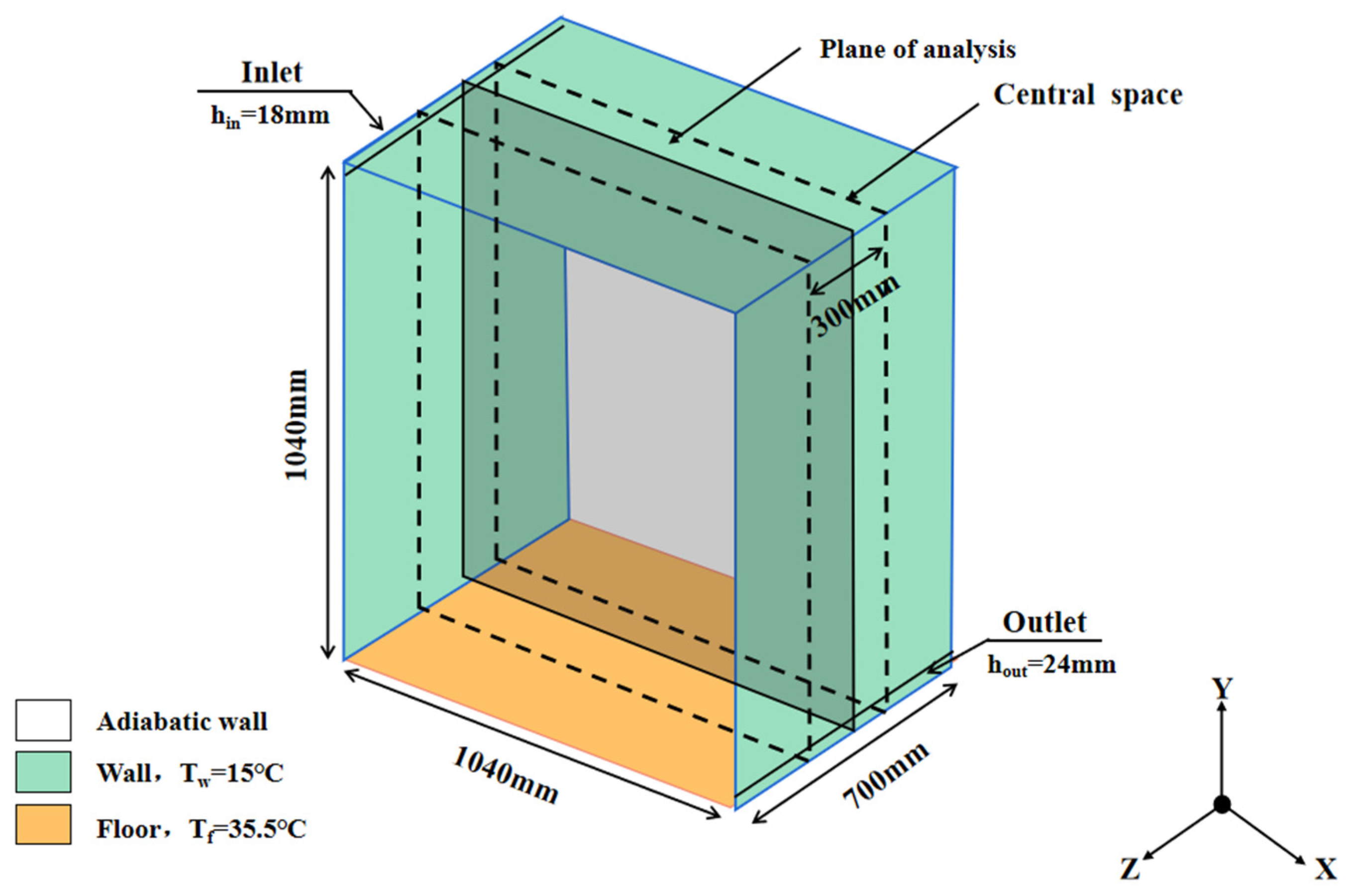
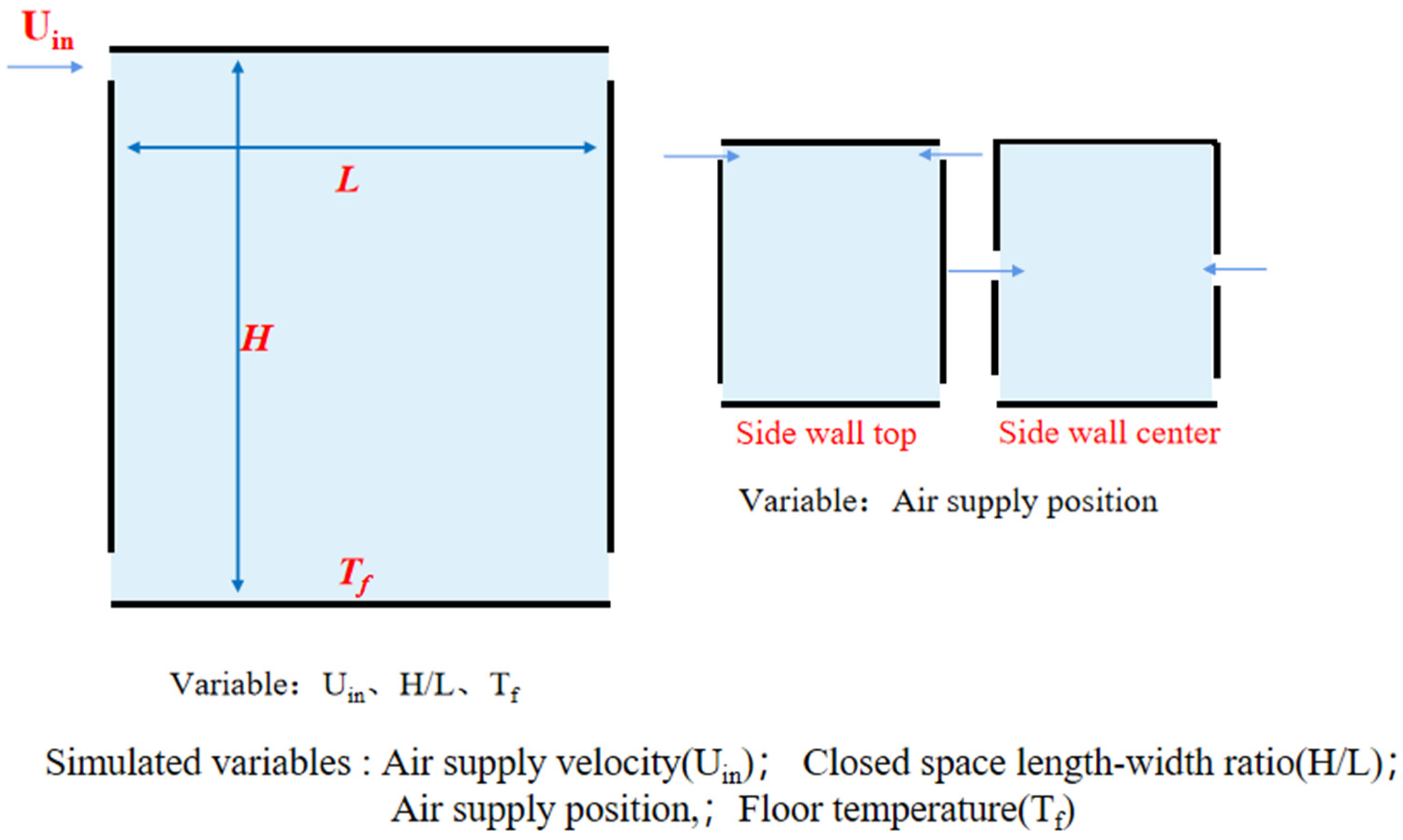
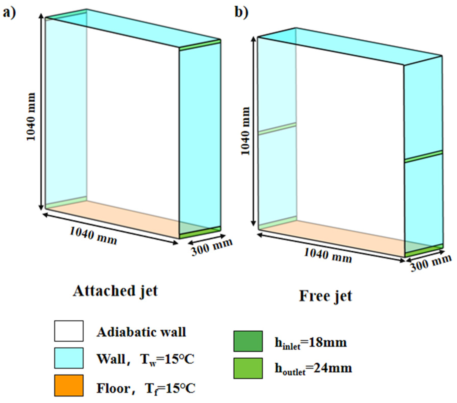
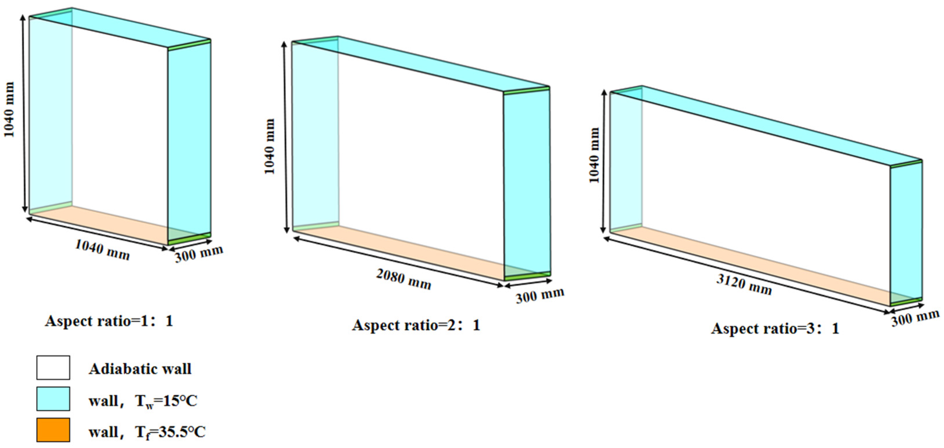
3.1. Geometric Model

The closed space was divided into three smaller spaces: one central working space where the measurements were performed and two guard spaces where the same flow as in the working cavity was simulated. The computational domain was created only for the central working space because it not only eliminates the thermal effect but also ensures good flow in the central working space. The air inlet in the closed central space was 300 mm long and 18 mm wide, and the air outlet was 300 mm long and 24 mm wide. The air supply vents, return air vents, and wall surface temperatures were configured to precisely match the experimental setup parameters. The model is shown in Figure 2.

3.2. Boundary Conditions

The boundary conditions in the CFD simulation were set to be consistent with the boundary conditions used in the experiments. The inlet air temperature was T_in is 15 °C, and the outlet air was set to zero static pressure. The air supply vents, return air vents, and wall surface temperatures were configured to precisely match the experimental setup parameters. The two sidewalls were set as adiabatic walls, i.e., the heat flux was zero (zero heat flux condition). All the walls were set as nonslip smooth walls. An experiment was conducted to eliminate the radiation effects between walls, so the radiative heat transfer and conductive heat transfer between surfaces were not considered. The inlet velocity and turbulence intensity remained consistent with the experimental configuration. The corresponding hydraulic diameter (D_h) was specified as 0.0035 m. The specific parameter settings are shown in

Table 1. All the change in parameters.

Case	Supply Air		Air Velocity (m/s)				Aspect Ratio of the Enclosed Space			Ground Temperature (°C)
	Attached jet	Free jet	0.57	0.85	1.28	1.92	1:1	1:2	1:3	15	25	35
Case 1	√		√	√	√	√	√			√
Case 2	√	√			√		√			√
Case 3	√		√				√	√	√	√
Case 4	√		√				√			√	√	√

.

3.3. Solver Settings

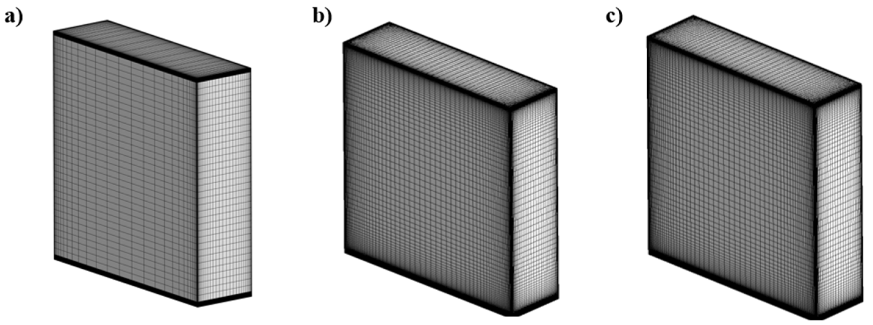
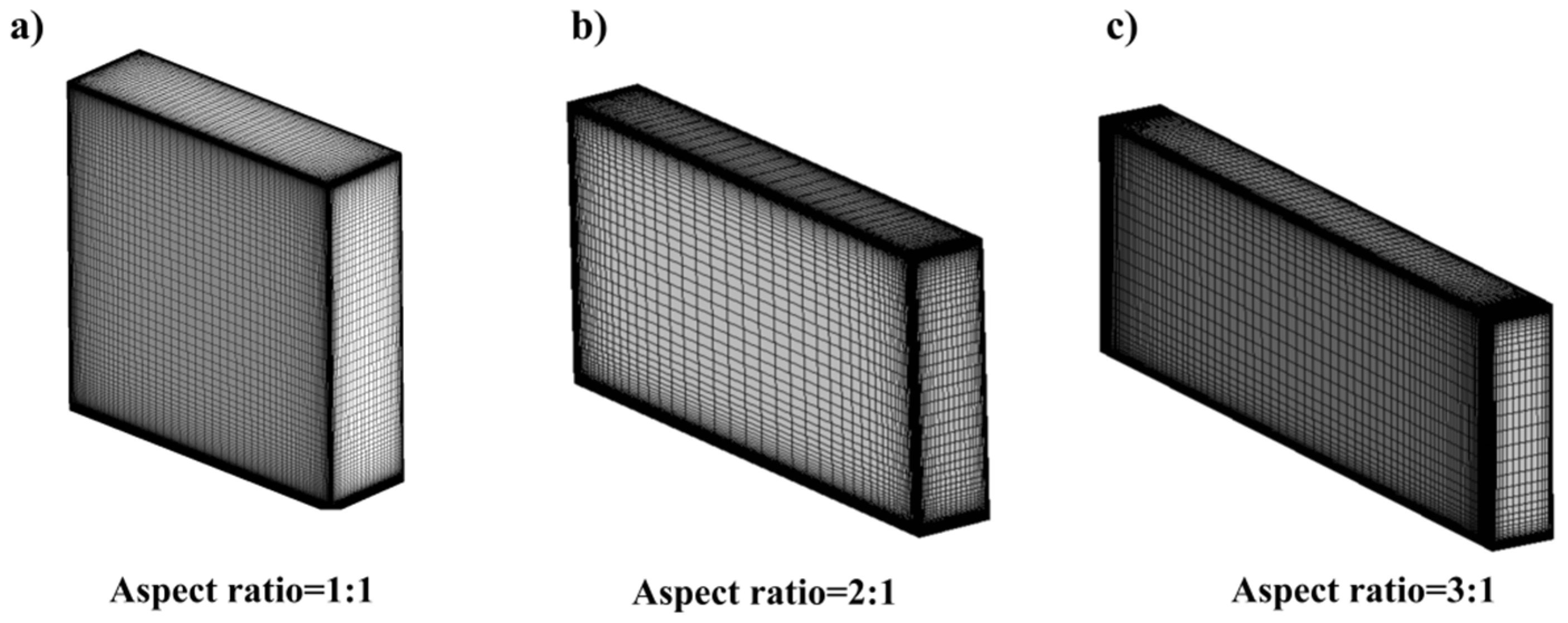
The fluid medium is air, and the turbulence model adopted is a large eddy simulation (LES). Due to the unknown sub grid-scale stresses generated by the filtering operation in LES models, the sub grid-scale model is set to the wall-adapting local eddy viscosity model. Due to the small diffusivity of the second-order discrete scheme, it was necessary to select a discretization scheme with at least second-order accuracy to overcome diffusion. This paper employs a second-order upwind scheme for the convection term, viscous term, and pressure interpolation term within the governing equations. The energy equation and momentum equation were both discretized using the bounded central differencing scheme. For the control equations governing fluid flow inside the cavity, the Boussinesq assumption was employed to handle the buoyancy force caused by temperature differences. When the residual values reached a steady state, the computations were considered to have converged. The residual convergence value for continuity, turbulent dissipation rate, turbulent kinetic energy, and velocity components were set at 10⁻⁵, while that of the energy was set at 10⁻⁶. In the case of reasonable grid accuracy, the PISO algorithm was found to have higher precision than the SIMPLE algorithm, because article chooses the PISO algorithm. The time step was set at 0.05 s. Numerical simulations were conducted by Ansys Fluent 19.0.

3.4. Grid

To reduce the number of grids and computational cost, the computational domain is set to the central working cavity. Because finer grids need to be used for large eddy simulations, this paper uses structured grids. To determine the independent solution of the grid, three grids were generated as shown in Figure 3, including 93,012, 122,771 and 330,423 elements, respectively. By adding the boundary layer grid and encrypting it, an accurate capture of the flow field is realized. Control y⁺ within 5.

Table 2. The maximum grid size and Y+ corresponding to different grid types.

Grid
Y+	Coarse	Basic	Fine
Maximum	5.1	3.4	2.8
Average	1.6	1.0	0.6

describes the maximum mesh size and Y+ corresponding to different mesh types.

The statistical average values of the unsteady calculation results after reaching stability were calculated and were compared with the experimental values. The numerical temperature and velocity on the horizontal centerline (Y is 0.52 m) and the vertical centerline (X is 0.52 m) were compared with experimental values. Figure 4a shows the dimensionless horizontal centerline velocities of the simulated and experimental values under grid elements 93,012, 122,771, and 330,423. The calculated mean deviations are 0.019, 0.005, and 0.009, respectively. Figure 4b shows the dimensionless vertical centerline velocity profile of three grid cells, and the average calculation deviations are 0.021, 0.007, and 0.035, respectively. Figure 4c shows the dimensionless vertical centerline temperature of the three grid units, and the average calculation deviations are 0.555, 0.003, and 0.807, respectively. Figure 4d shows the dimensionless vertical centerline temperature of the simulated and experimental values for grid numbers 93,012, 122,771, and 330,423, and the calculated mean deviations are 0.53, 0.05, and 1.34, respectively. When the grid number is 122,771, the simulation results are in good agreement with the experimental results. Through the above verification, the model is found to be suitable for large eddy simulation of 122,771 grid units. Therefore, in the following example, 122,771 is used for mesh CFD simulation analysis.

3.5. Numerical Case Setup

Based on the study of Blay et al. the air supply configuration was modified from a single inlet and single outlet to dual inlet and dual outlet as shown in Figure 5, while keeping the other boundary conditions constant. The LES method was used to simulate the opposed jets in the enclosed space. The instability of the airflow structure was analyzed by varying different parameters. The airflow influencing parameters included the air supply velocity, position of the air inlets, aspect ratio of the enclosed space, and thermal plume. The specific simulation variables are shown in Figure 5. The first case was the influence of different air supply velocities on the airflow structure under isothermal conditions, where the ground temperature is equal to the wall temperature, with a supply angle of φ is 0° and a constant air supply rate. Four velocities, 0.57 m/s, 0.85 m/s, 1.28 m/s, and 1.92 m/s, were selected for the simulation analysis. To maintain a constant airflow rate, the corresponding inlet heights for the four air supply velocities were set at 18 mm, 12 mm, 8 mm, and 5.3 mm, respectively. The second case simulates the airflow field at different locations of the air inlet under isothermal conditions and with a constant air supply velocity of U_in is 1.28 m/s and a supply angle of φ is 0°. Specifically, two air supply configurations were adopted: upwards supply and downwards return and central supply and downwards return (free jet). The third algorithm investigates the effect of different spatial aspect ratios on the flow field under isothermal conditions, with a fixed air supply velocity and supply angle. Three enclosed space aspect ratios, namely, 1:1, 1:2, and 1:3, were selected for instantaneous airflow field measurements. The fourth case investigates the effect of different ground temperatures on the flow field with an air supply velocity of 0.57 m/s and a supply angle of 0°. Ground temperatures of 15 °C, 25 °C, and 35 °C were selected as the respective boundary conditions for the simulation.

Due to the temporal variation in the unsteady airflow structure within an enclosed cavity, this study investigates the velocity time series results of the unsteady airflow structure. A qualitative analysis of the velocity contour was conducted at the central section (Z is 0.15 m) of the enclosed cavity. Additionally, the velocity time series at the coordinates (0.52, 0.52, 0.15) in the center of the cavity were monitored.

To facilitate analysis, normalize the airflow velocity in the flow field:

$$u={\displaystyle \frac{U}{U_{in}}}.$$

(1)

In the formula, U is the normalized velocity, u is the airflow speed in the flow field, m/s, and U_in is the air supply speed, m/s.

4. Result Analysis

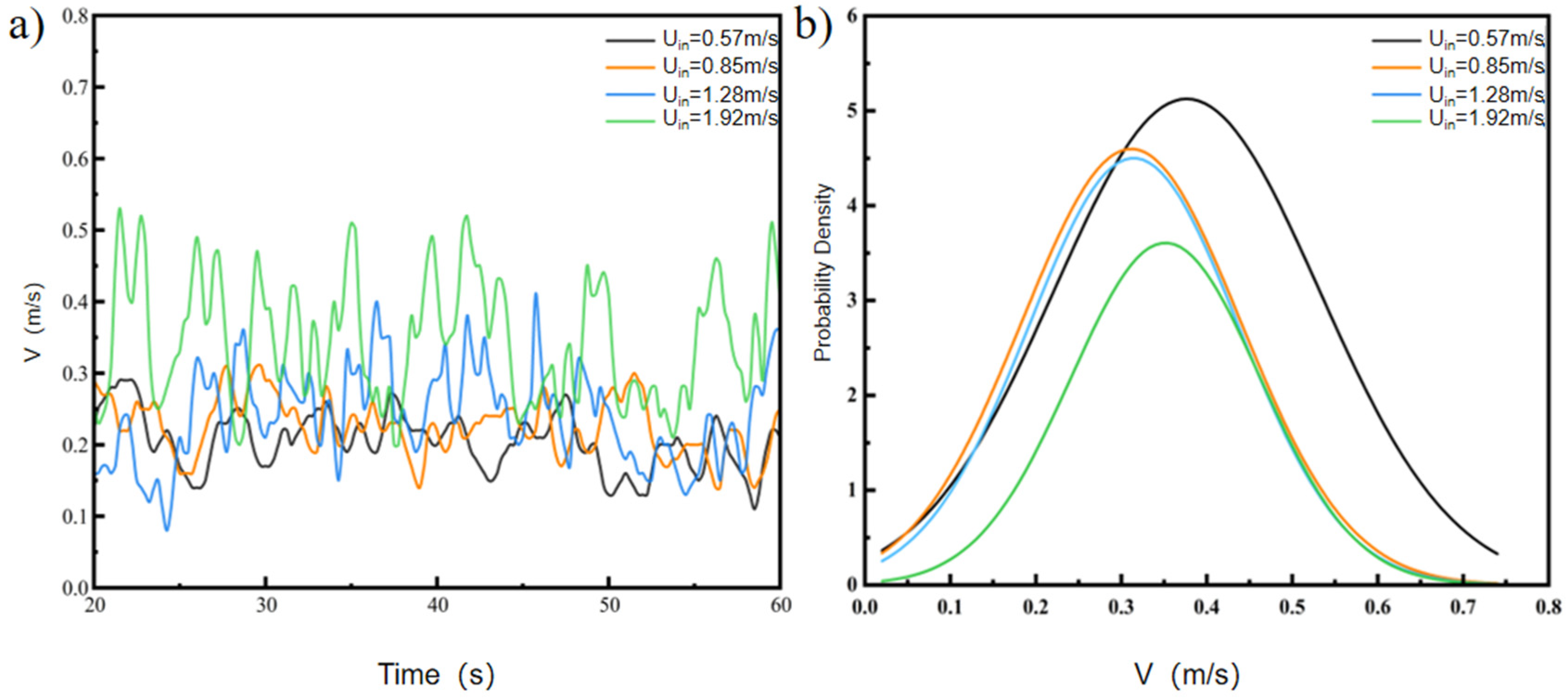
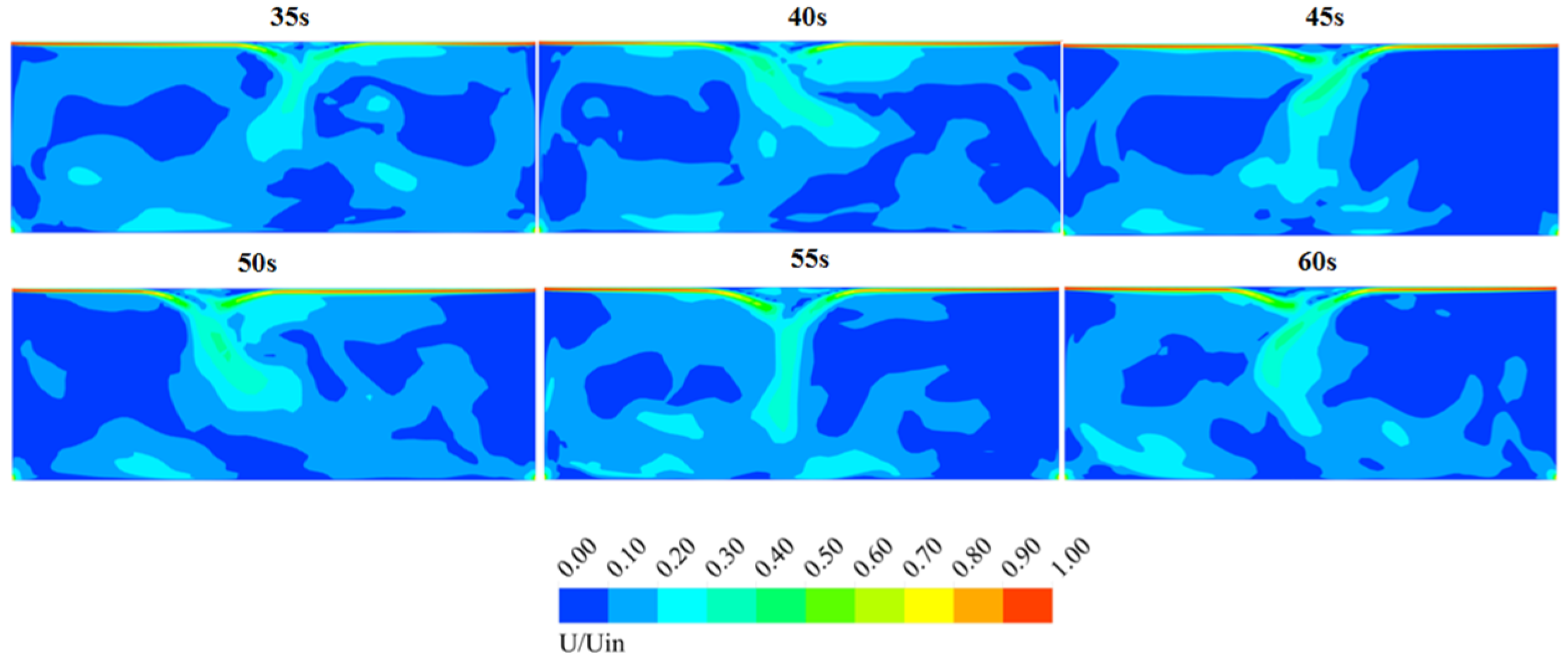
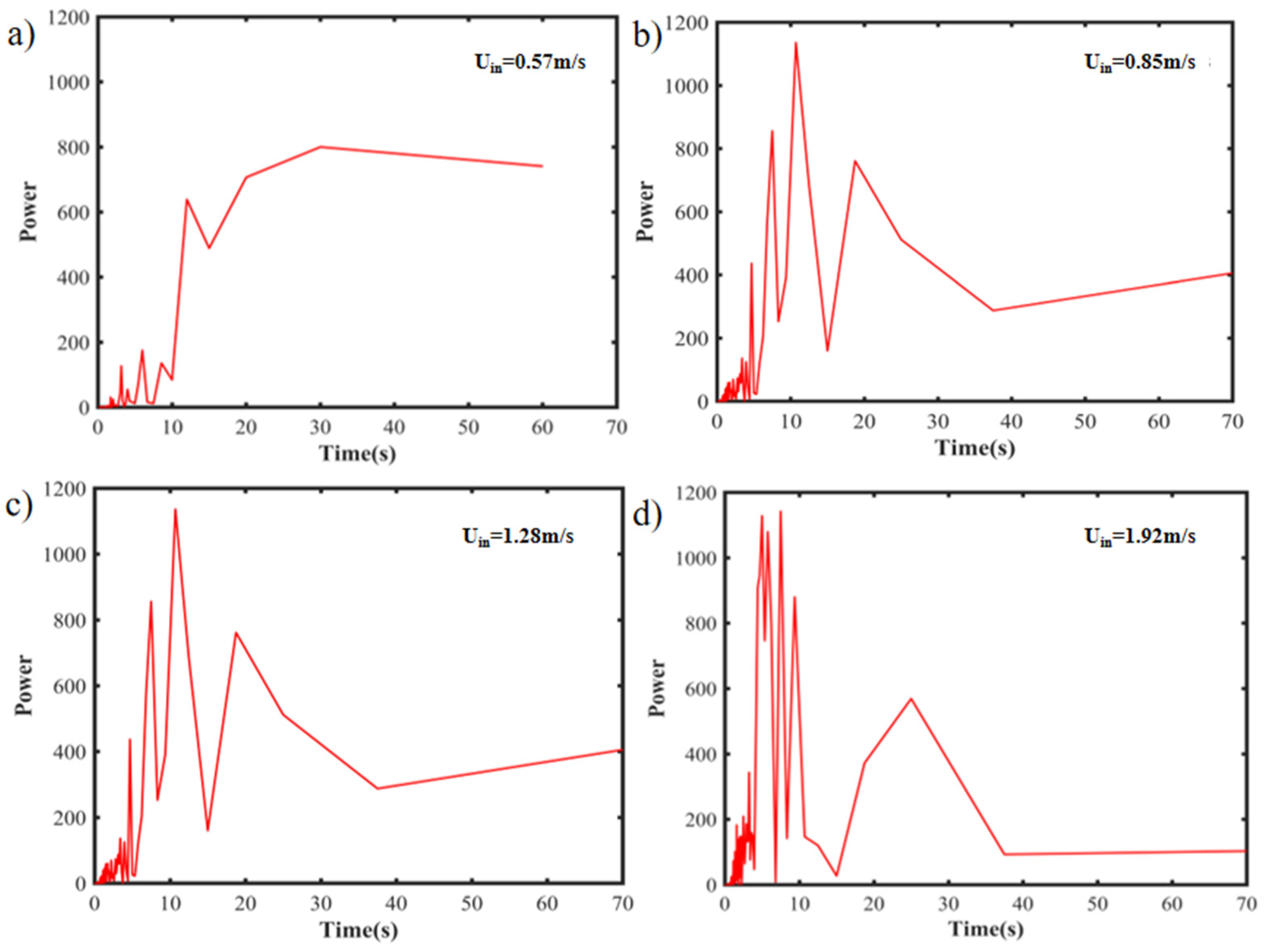
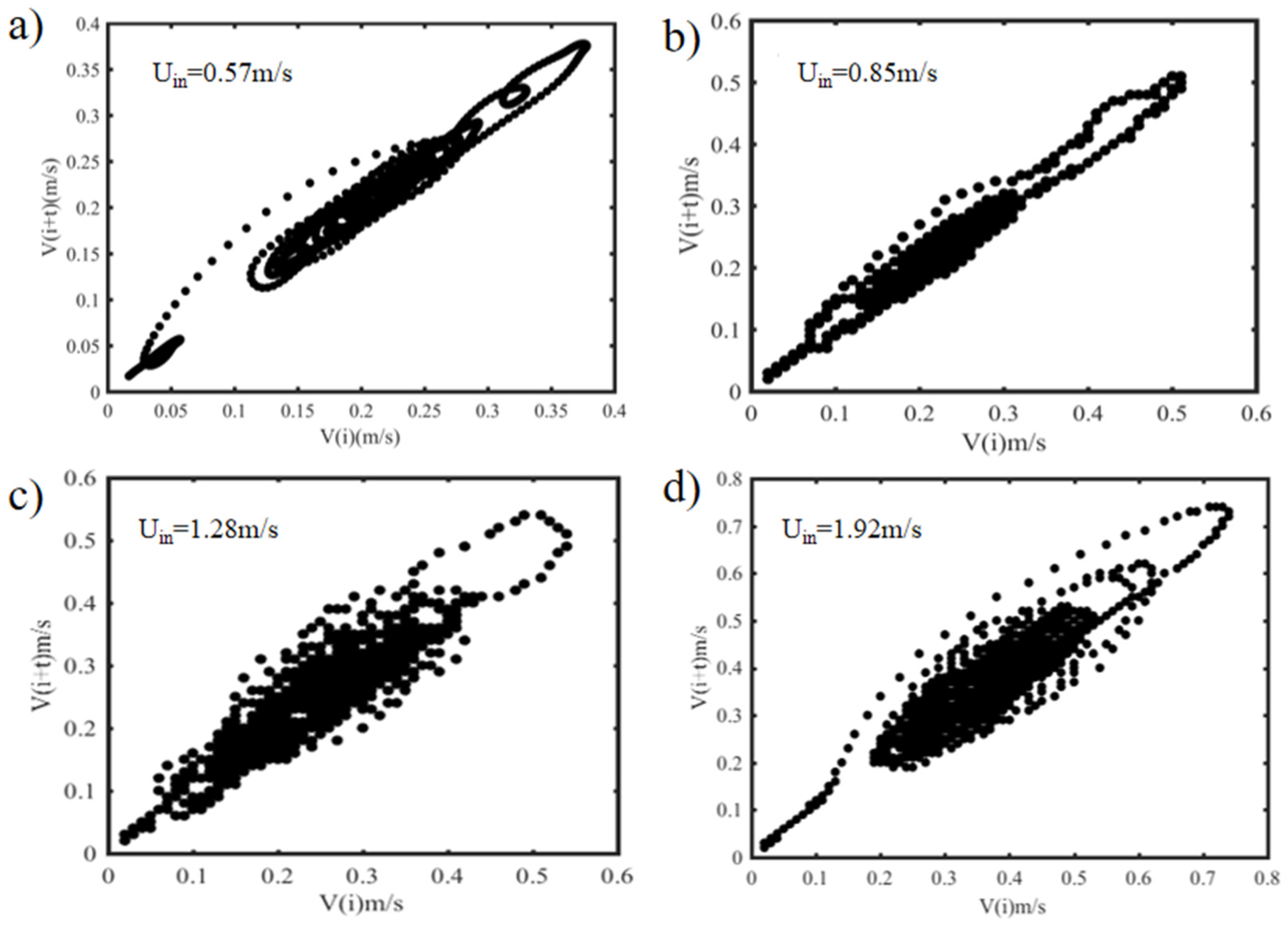
4.1. Different Air Supply Velocities

The influence of the air supply velocity on the instantaneous airflow structure was studied under isothermal conditions with air supply angle was 0°. Figure 6 shows the transient flow field contour plot at the cross-section z is 0.15 m under different air supply velocities. A constant air supply rate was ensured by changing the height of the air inlet during this process. The two jets facing the opposite inlet collide in the cavity, and the air flow swings, showing an asymmetrical phenomenon. Figure 7 shows the monitoring curve of the 20 s~60 s velocity time series at the cavity center point (0.52, 0.52, 0.15) and the velocity probability density distribution at the center point. As the air supply velocity increases, the swing amplitude of the airflow structure decreases, and the small-scale airflow around the airflow decreases. It can be seen from Figure 7a that when the air supply velocity is 0.57 m/s, the speed range is distributed between 0.15 m/s–0.29 m/s.

When the air supply velocity is 1.28 m/s, the velocity range is distributed between 0.10 m/s–0.35 m/s. When the velocity increases to 1.92 m/s, the velocity range is distributed between 0.15 m/s–0.51 m/s. The time interval between the maximum speed and the minimum velocity of air flow at the monitoring point is reduced from 8 s to 3 s. The data indicate that as the air supply velocity increases, the airflow swing frequency increases. It can be seen from Figure 7b that as the air supply velocity increases, the probability of the concentrated distribution range of air flow velocity at the monitoring point decreases, the amplitude of air flow swing decreases, and the air flow oscillation gradually stabilizes.

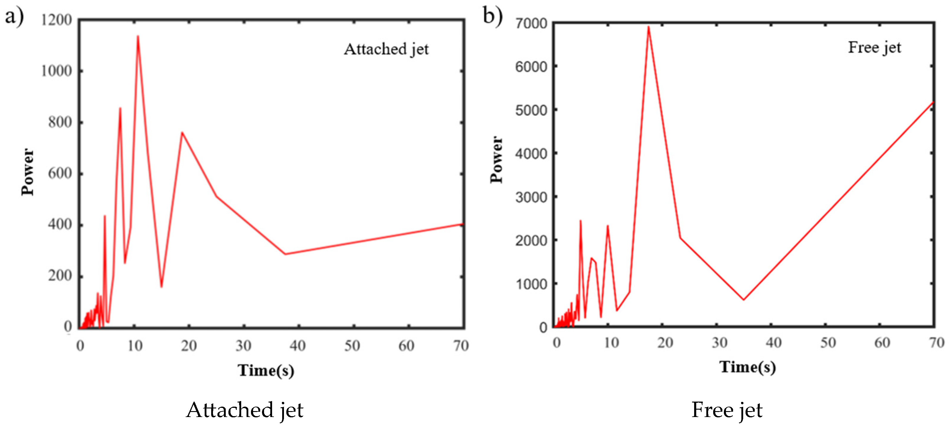
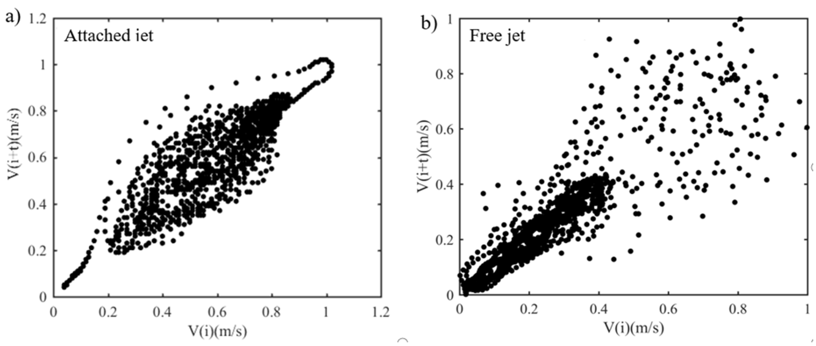
4.2. Impact of Air Supply Positions

The effect of different air supply positions on the transient airflow structure was studied when the isothermal air supply angle was 0° and the air supply velocity was 1.28 m/s. This paper studies the influence of the air supply position on the airflow structure of the enclosed space at the top of the cavity side wall and the middle of the side wall. The three-dimensional diagrams of the two air supply locations are shown in Figure 8. The model is meshed, and the number of mesh divisions is shown in Figure 9.

Figure 10 shows the transient flow field at different air supply positions with an air supply velocity of 1.28 m/s. When the air supply positions are located at the top of the side wall, the two jets collide in the cavity and the airflow swings, showing an asymmetrical phenomenon. When the air supply position is located at the center of the side wall, after the two jets collide, at different times, a jet deflects toward the ground, the deflection of another jet towards the top of the cavity. Moreover, during the jet deflection process, the surrounding small-scale airflow structure increases.

Figure 11 shows the monitoring curve of the 20 s~60 s velocity time series at the cavity center point (0.52, 0.52, 0.15) and the velocity probability density distribution at the center point. The air supply position is located at the top of the side wall, the velocity fluctuation at the monitoring point is small, and the velocity range is 0.15 m/s~0.37 m/s. The time interval between the maximum speed and the minimum speed of the airflow at the center point is 3 s. When the air supply position is located at the center of the side wall, the velocity at the center point fluctuates greatly, with the velocity concentrated at 0.05 m/s~0.7 m/s. The amplitude of the airflow swing is large, and the time interval between the maximum and minimum airflow speed at the center point is 7 s. It can be seen that when the air supply position is located at the center of the side wall, the airflow oscillation amplitude at the center point increases and the airflow swing frequency decreases. When the air supply position is at the center of the side wall, it can be clearly seen that there is a large peak value in the instantaneous velocity of the center point at 65 s, with a velocity of 0.67 m/s. Combined with the velocity cloud chart at 65 s, the data indicate that when the center point velocity peaks, the airflow on both sides will re-enter a transition state. The airflow on the right side suppresses the airflow on the left side, gradually causing the airflow on the left side to deflect toward the top. When the left airflow is completely deflected, the center point velocity decreases again.

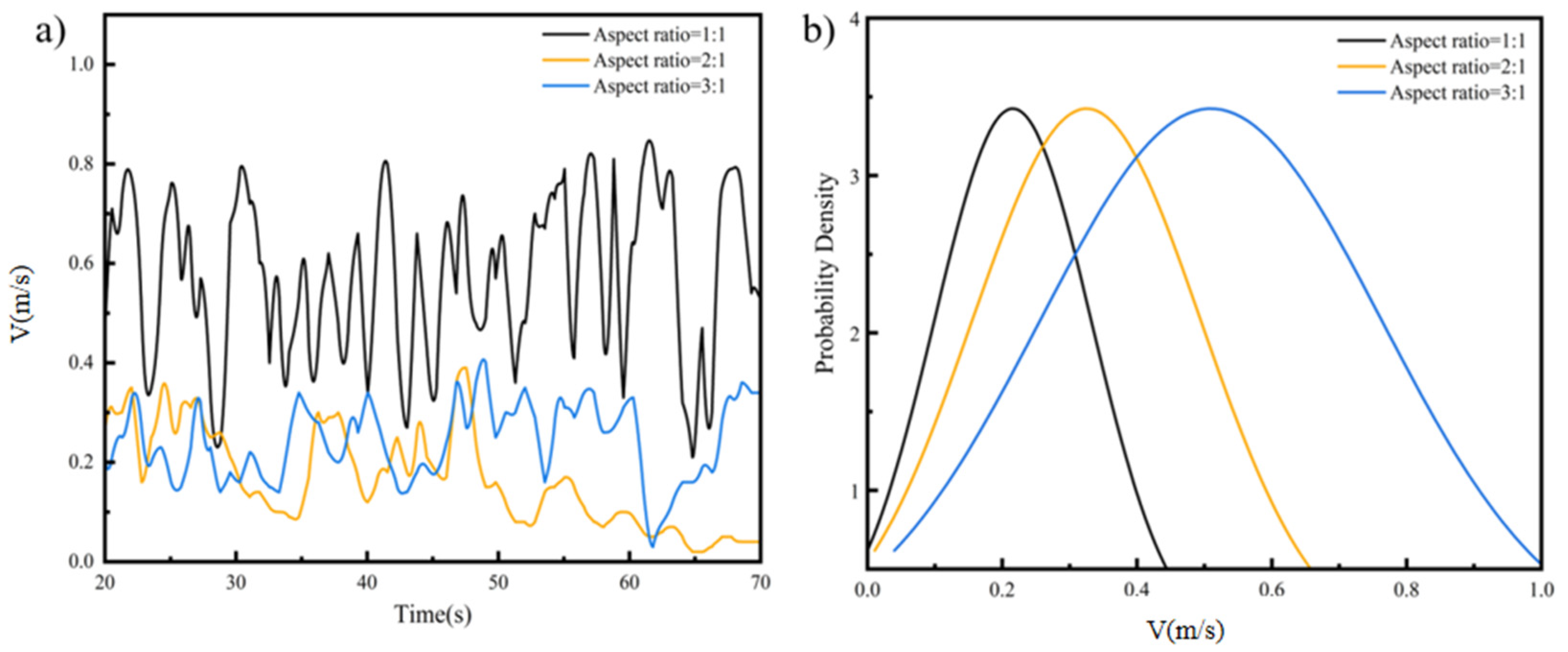
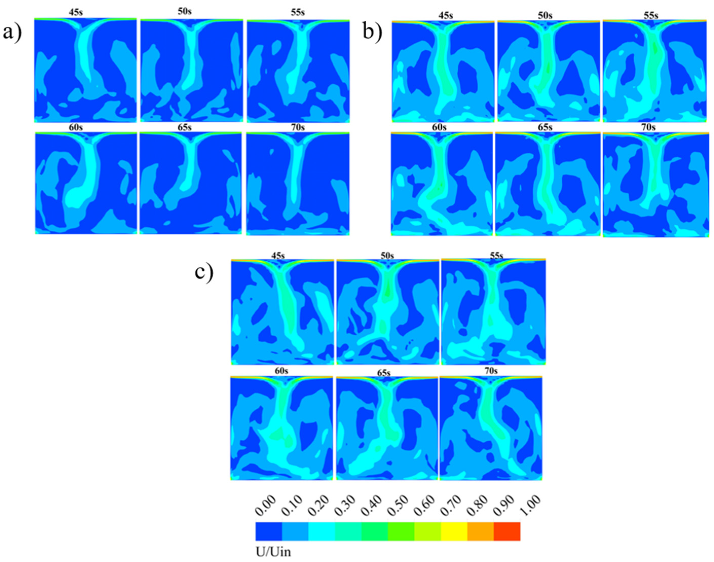
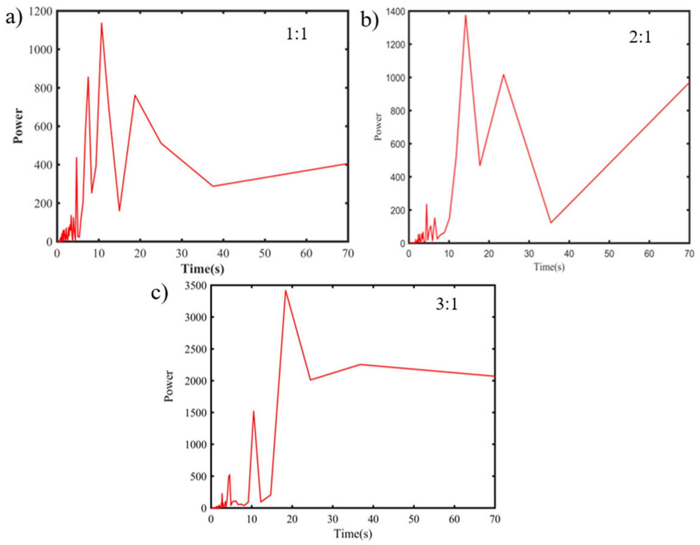
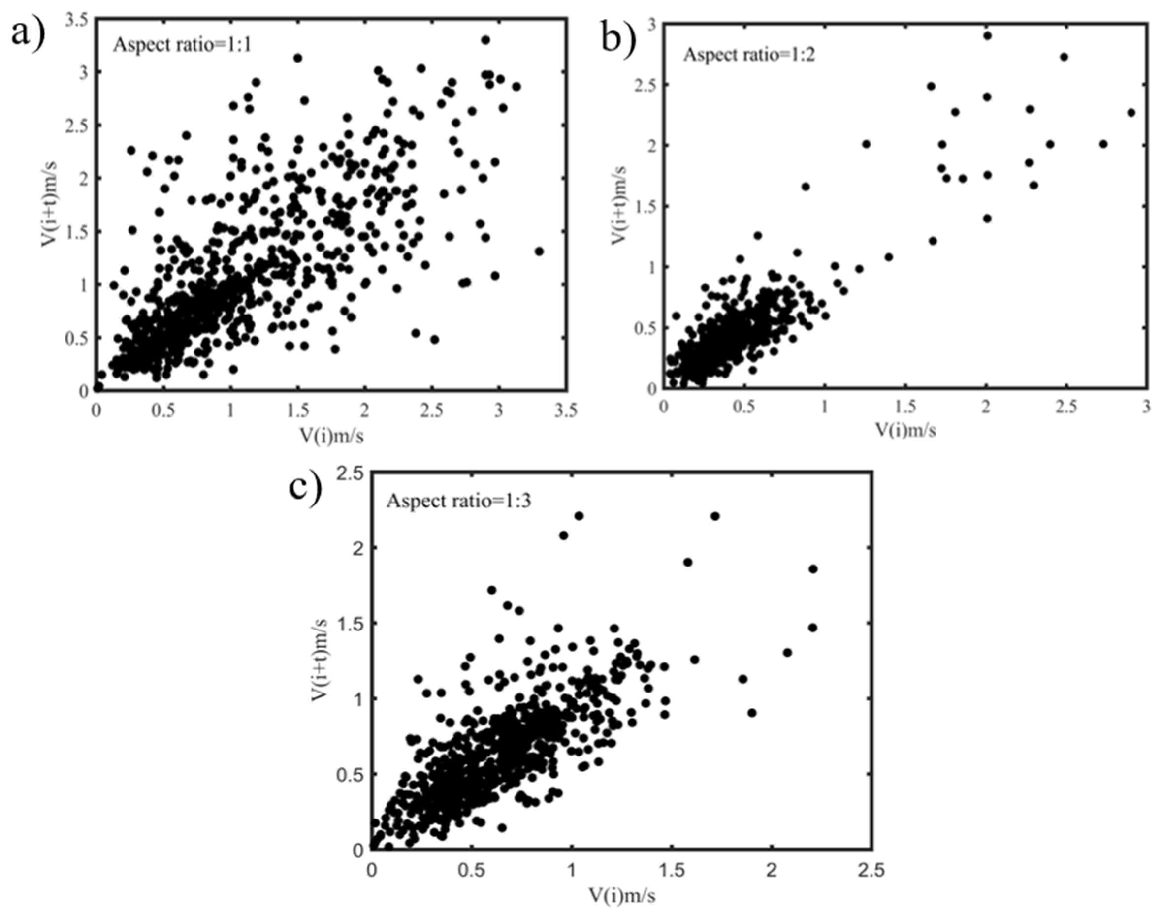
4.3. Impact of the Aspect Ratio

The effect of different closed space aspect ratios on the transient airflow structure was studied when the isothermal air supply angle was 0° and the air supply speed was 1.28 m/s. Enclosed spaces with different aspect ratios are shown in Figure 12. The closed spaces with three aspect ratios are meshed, and the number of grid divisions is shown in Figure 13.

Figure 14, Figure 15 and Figure 16 is a transient flow field diagram with different aspect ratios of 1:1, 1:2, and 1:3 at section z is 0.15. It can be seen from the figure that as the aspect ratio increases, the distance of the airflow jets on both sides increases. After the jets on both sides collide, one side of the airflow sweeps the surrounding small airflow structure and suppresses the other side of the airflow from flowing to the sidewall. For example, when the aspect ratio is 2:1 and when the airflow collides, the right airflow suppresses the left airflow, causing the airflow to move to the left and deflect. In the transition state, the airflow moves to the center of the closed cavity, and then the left airflow suppresses the right airflow from moving to the opposite sidewall. Moreover, an increase in the aspect ratio affects the distance of the air flow to the bottom of the closed cavity. This may be due to the increase in the small-scale air flow with the increase in the jet distance from the initial to the collision process of the air flow on both sides, which affects the deflection of the air flow, resulting in a shorter distance of the air flow to the bottom.

Figure 17 shows the monitoring curve of the 20 s~60 s velocity time series at the cavity center point and the velocity probability density distribution at the center point. When the aspect ratio is 1:1, the speed is concentrated in the range of 0.28 m/s~0.8 m/s. When the aspect ratio is 3:1, the speed range is concentrated in the range of 0.1~0.4 m/s. With increasing length-to-width ratio, the velocity fluctuation amplitude decreases, which indicates that an increase in the length-to-width ratio leads to an increase in the airflow swing period. Combined with the above cloud images, when one side of the airflow suppresses the other side of the airflow to move to the sidewall, the fluctuation amplitude of the velocity at the collision point gradually decreases. Additionally, there is periodicity and instability in the airflow oscillation under different aspect ratios.

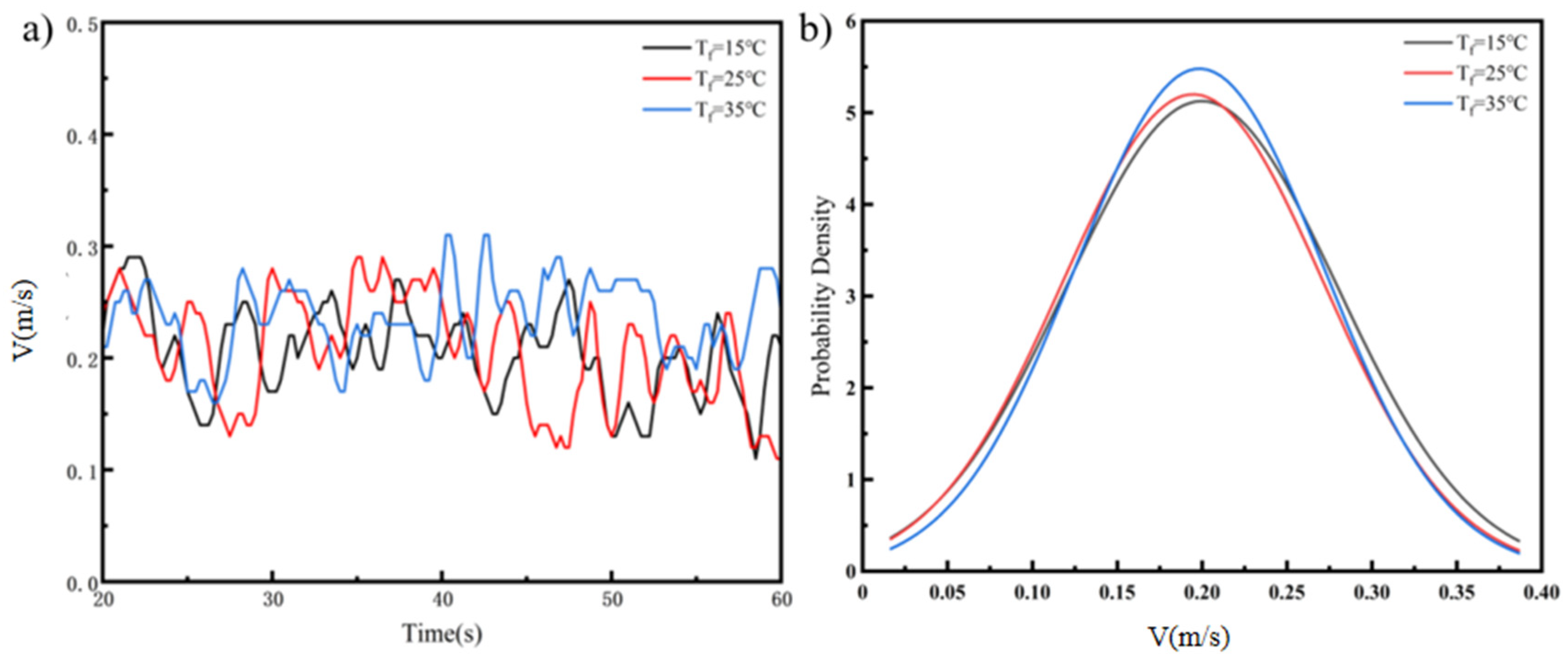
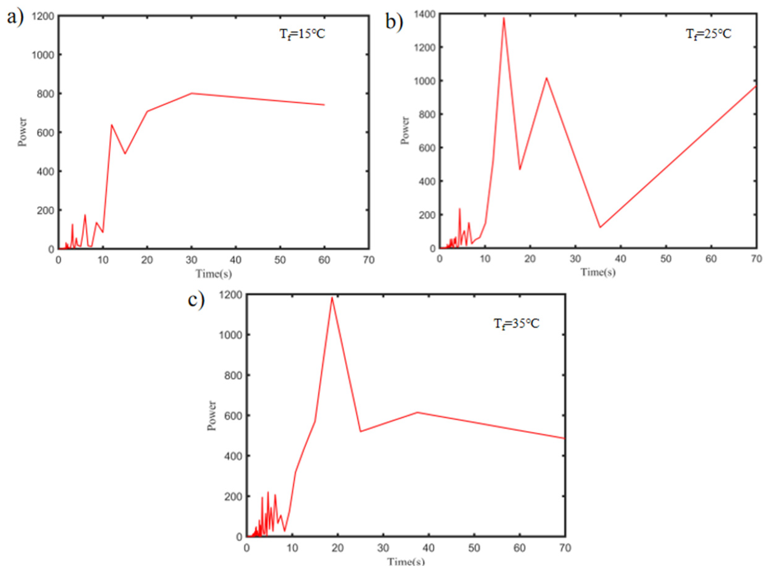
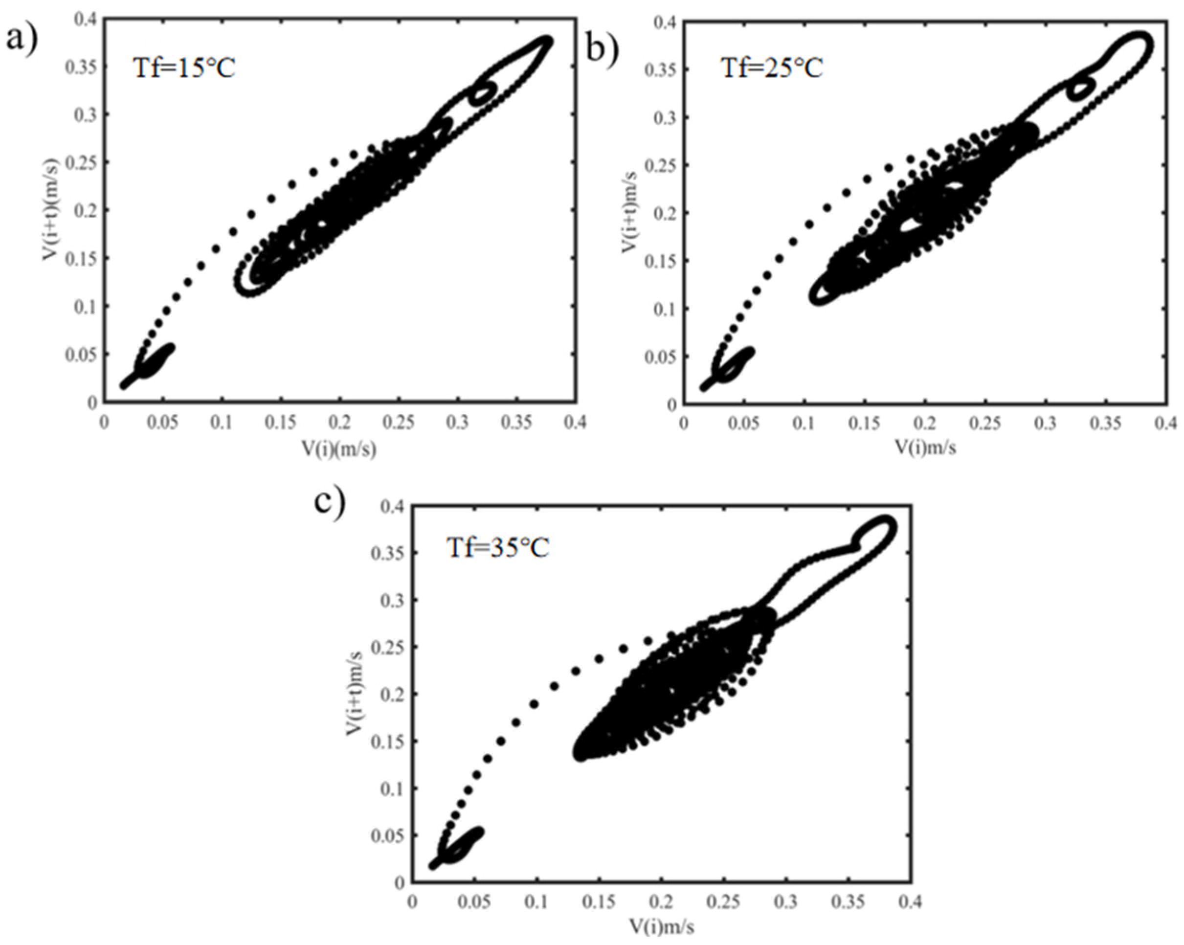
4.4. Impact of Floor Temperature

The above studies were carried out under isothermal conditions. Previous research has shown that the heat source temperature also affects the deflection of airflow structures. Therefore, to ensure the same air supply speed and air supply angle, this paper studies the transient airflow structure when the floor temperature is heated to 15 °C, 25 °C and 35 °C. The airflow distribution is different from that under isothermal conditions. Under non-isothermal conditions, the airflow structure diffuses upwards due to the influence of the floor heat source temperature. As shown in Figure 18, the velocity cloud diagram at cross-section Z is 0.15 is analyzed. The diagram shows that the jet deflects after the collision. Under the action of the heat source temperature, the up- and down-oscillation of the airflow is suppressed. When the floor temperature increases from 15 °C to 35 °C, the dynamic airflow structure gradually becomes confused. The diffusion of the airflow to the surrounding area obviously drives the deflection of the jet after the collision to be more obvious, and the airflow bifurcation is more refined. The dynamic airflow structure at different heat source temperatures shows periodic changes.

It can be seen from Figure 19 that when the heat source temperature is the highest, the speed fluctuation range of the monitoring point is 0.14 m/s~0.28 m/s. Under isothermal conditions, the velocity fluctuation range of the monitoring points is 0.1 m/s~0.32 m/s. The larger the heat source temperature is, the smaller the velocity fluctuation at the monitoring point is. This is because when the heat source temperature exists, the airflow diffuses everywhere, forming a vortex airflow distribution, resulting in the airflow at the center point becoming a small airflow organization, and the velocity fluctuation changes more gradually. Figure 19 also shows that the airflow structure experiences a certain period. When the local plate temperature is heated to 35 °C, the period of the central monitoring point is clearly longer than that for a floor temperature of 15 °C.

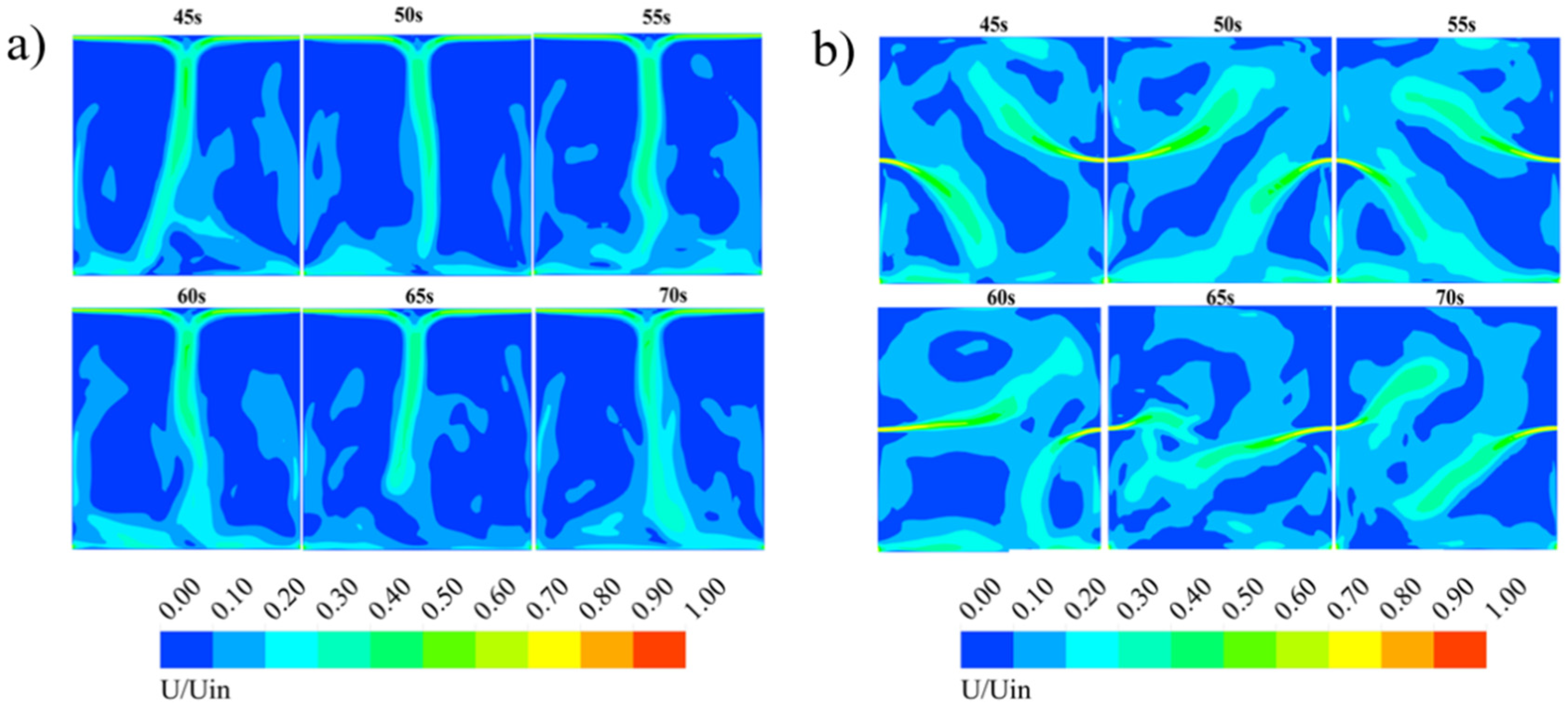
4.5. Periodicity Analysis

From the above analysis, it is obvious that the airflow oscillation in the central cavity is periodic under different parameter settings. However, the specific period cannot be obtained from the velocity cloud diagram or velocity monitoring sequence. Therefore, to analyze the periodic characteristics of the velocity time series under an unsteady flow field, the energy spectrum is used for analysis. This paper uses the power spectrum method for analysis and calculation and deduces the calculation. Airflows oscillate during specific periods. The specific derivation calculation process is as follows:

Let u(i) be a part of time series u(i), i is 1, 2, …, I. For the fast Fourier transform of the velocity time series, the calculation formula can be based on (2):

$$F\left(k\right)={\displaystyle {\sum }_{i=1}^I}u(i)e^{-\int 2\pi (k-1){\displaystyle \frac{i-1}{i}}}.$$

(2)

After the velocity time series is transformed, the frequency is $f_i=2\mathsf{\pi }{\displaystyle \frac{i-1}{I}}$, where i = 1, 2, …, is the maximum amplitude of the fast Fourier transform of the average period and the reciprocal of the corresponding frequency is the power. It is calculated using Formula (3):

$$P={\displaystyle \frac{1}{max[F\left(1\right),F\left(2\right),\dots ,F(I\left)\right]}}.$$

(3)

The air supply velocities considered in the study are 0.57 m/s, 0.85 m/s, 1.28 m/s, and 1.92 m/s. The power spectrum distribution is depicted in Figure 20, where the horizontal axis represents time and the vertical axis represents power. Due to the periodicity of the small-scale airflow structure, multiple small peak powers can be observed in the graph. This suggests the presence of multiple periodicities in the small-scale airflow. Using the power spectrum method, the period of air flow oscillation in the cavity was calculated for a wind speed of 0.57 m/s. With an increase in the wind speed to 0.85 m/s, the period of air flow oscillation in the cavity was determined to be 11.3 s. Based on the power spectrum analysis, the air flow oscillation period was calculated to be 10.6 s for an inlet velocity of 1.28 m/s. Furthermore, as the air supply velocity increases to 1.92 m/s, the airflow oscillation period is shortened to 7.7 s. Figure 12 shows that with increasing inlet velocity, the period of air flow oscillation in the cavity becomes increasingly obvious, and the disturbance of small-scale air flow becomes increasingly less obvious. This is because when the air inlet velocity increases, the impact of the jet after the collision increases, and the airflow distribution is concentrated, so the small-scale airflow structure is less distributed.

Figure 21 shows the power spectrum distributions under the different air supply modes. When the air supply is the upper supply and lower return, the airflow oscillation period in the closed cavity is 10.6 s. When the air supply is the middle supply and lower return, the airflow oscillation period is 15.6 s. The airflow oscillation period of the free jet formed by the middle feed and lower return is longer than that of the attached jet formed by the upper feed and lower return. This is because in the free jet, the collision and deflection of the two airflows lead to an increase in the surrounding small-scale airflow structure, and the small-scale airflow period is increased by 0~10 s, thus affecting the overall airflow oscillation period.

The power spectrum is used to analyze the airflow oscillation under different aspect ratios. The airflow oscillation with different aspect ratios in the closed space is periodic. When the aspect ratio is 1:1, the airflow oscillation period is 10.6 s. When the aspect ratio is 2:1, the oscillation period is 14.5 s. When the aspect ratio is 3:1, the period is 18.1 s. Periodic distribution of different aspect ratios as shown in Figure 22. As the aspect ratio increases, the airflow oscillation period increases. This is because in the process of jet collision, an increase in the length-to-width ratio leads to an increase in the jet distance, an increase in the surrounding small-scale airflow, and the continuous entrainment of the surrounding airflow to the collision center. The longer the jet distance is, the longer the movement time of the surrounding small airflow to the collision center, thus affecting the oscillation period of the airflow.

Figure 23 shows the power spectrum distributions at different heat source temperatures. The horizontal and vertical coordinates represent time and power, respectively, and the airflow oscillation period changes with the change in heat source temperature. When the heat source temperature is 15 °C (isothermal condition), the period of airflow oscillation is 11 s. When the temperature of the heat source increases to 25 °C, the period of airflow oscillation in the cavity becomes 13 s. When the heat source temperature is heated to 35 °C, the oscillation period of airflow in the cavity becomes 17 s. Figure 24 shows that when the heat source temperature increases from 15 °C to 35 °C, the period of airflow oscillation in the cavity becomes longer. This is due to the influence of the ground source temperature. After the two airflows collide with the jet, a small airflow structure is formed on both sides. These small airflow structures are continuously entrained on both sides, lengthening the airflow swing period and indicating that the heat source temperature has a significant effect on the airflow distribution.

4.6. Phase Space Reconstruction Analysis

To investigate the instabilities of flow field structures, this study employs a phase space reconstruction method to analyze the non-stationarity of time scales in flow field structures. By reconstructing the unsteady time series into low-order nonlinear sequences in phase space, the sequence is transformed into describable states, facilitating the discovery of its variation patterns.

According to the Takens F [41] mathematical theory, it is assumed that the one-dimensional univariate time series is shown as follows:

$$x_i=(x_1,x_2,\dots ,x_N).$$

The m-dimensional vector is formed by the time delay $X_i=[x_1,x_2,\dots ,x_{i+(m-1)\tau }]$, where X_i is the reconstructed vector, m is the embedding dimension, and τ is the delay time. If N is one-dimensional univariate data, then i = 1, 2, …, M; m = N − (M − 1) τ, the number of phase points of the phase space vector after M reconstruction. In phase space reconstruction, Takens’ theorem states that for an ideal one-dimensional time series without noise, with arbitrary values for the embedding dimension m and delay time interval τ, there is a certain amount of noise in the actual measured time series. Therefore, the delay time interval and embedding dimension of the phase space reconstruction are taken into account.

In this study, two-dimensional phase space reconstruction is analyzed. According to the theory of phase space reconstruction, when the sampled signal is completely random white noise, its phase space reconstruction diagram fills the whole phase space. When the sampled signal is a chaotic signal, its phase space shows a certain shape, and different laws have different shapes [42], Research in the literature shows that two-dimensional phase space reconstruction diagrams of natural wind and mechanical wind are spindle-shaped and elliptical, respectively, which shows that natural wind has stronger autocorrelation than mechanical wind [43]. In this paper, two-dimensional phase space reconstructions at the collision points of air flow with different air supply forms and different aspect ratios of closed space are analyzed.

The figure shows the reconstruction of the two-dimensional phase space reconstruction of the velocity time series of the collision point. The abscissa and ordinate represent the original time series and the reconstructed time series, respectively. When the air supply speed is 0.57 m/s, the phase space reconstruction diagram of the collision point reveals that the aggregated spatial points exhibit a spindle shape, indicating that there is a strong correlation. Most of the velocity distributions are between 0.1 m/s and 0.25 m/s. With increasing air supply velocity, the velocity range at the collision point increases, and the correlation decreases. The shape of the phase space diagram increases with increasing air supply speed, the width of the spindle gradually increases, and the spindle-shaped tail speed gradually disperses. This phenomenon indicates that with the change in the air supply speed, the airflow fluctuation increases after the collision, and the surrounding small-scale airflow structure increases, revealing the phenomenon of unstable oscillation of the airflow after the collision.

Figure 25 shows a two-dimensional phase space reconstruction diagram of the velocity time series of the collision points selected for the different air supply forms. The phase space reconstruction diagram of the collision point reveals that the aggregation space points are spindle-shaped, indicating that there is a strong correlation between the velocity sequences of the two air supply forms. When the air supply is an attached jet, the velocity range is concentrated from 0.1 m/s to 0.4 m/s. When the air supply is a free jet, the velocity is concentrated in the range of 0.1 m/s to 0.45 m/s. Compared with that of the attached jet, the speed of the spindle tail formed by the collision point of the free jet is more divergent after reconstruction, and these speed ranges are concentrated in the range of 0.6 m/s to 1 m/s. This phenomenon confirms that in the free jet, when the two airflows are deflected up and down, the velocity range of the collision point is small; however, when the two airflows are in the process of transition from collision to deflection, the velocity range of the collision point is large, reflecting the periodic deflection of the free jet airflow collision.

Figure 26 shows the reconstructed image obtained by two-dimensional phase space reconstruction of the velocity time series of collision points at different aspect ratios. As the aspect ratio increases from 1:1 to 3:1, the velocity range of the collision point is maintained at 0.1 m/s to 1 m/s. The aggregated spatial points exhibit a spindle shape, indicating that there is a correlation between the velocity time series at the collision point.

Figure 27 shows the two-dimensional phase space reconstruction of the velocity time series at different temperatures The reconstructed image is obtained by reconstructing the two-dimensional phase space of the collision point velocity time series at different ground source temperatures. The aggregated spatial points are spindle-shaped and exhibit obvious autocorrelation. With the increasing ground source temperature, the velocity increases from 0.1 m/s to 0.3 m/s. As the ground source temperature increases, the width of the spindle gradually becomes wider. This shows that an increase in temperature leads to an increase in small-scale airflow around the cavity, and the instability oscillation of airflow gradually becomes obvious. The effect of temperature on airflow instability in a closed cavity is revealed.

5. Discussion

Regarding the potential numerical errors and limitations of the adopted turbulence model, we have conducted the following discussion. Using the LES turbulence model, there are numerical errors in the prediction of anisotropic flows by the sub grid-scale (SGS) model. The model may fail to accurately capture the energy backscatter phenomenon from small to large scales. The LES turbulence model is limited by wall regions and high Reynolds numbers, and resolving the wall requires a significant increase in grid size, which in turn increases computational costs and loses the computational efficiency advantage.

Regarding the comparison between grid resolution and the established standard (e.g., Kolmogorov scale resolution), we have made the following specific discussion: In terms of grid resolution, the study ensured that y < 5 (average y ≈ 1) of the near-wall grid, thereby fully resolving the viscous sublayer and meeting the best practice standards for LES in wall flows. Although it is challenging to fully resolve the Kolmogorov scale in high Reynolds number flows, the grid resolution (Δx ≈ 5 mm) successfully captured more than 80% of the turbulent kinetic energy (TKE) spectrum, meeting the Pope criterion (Δ ≤ πη, where η is the Kolmogorov scale). This result was further verified by analyzing the energy spectrum attenuation in the inertial subregion. In addition, the power spectrum of the velocity fluctuations at the collision point exhibited the expected −5/3 slope in the inertial subregion, confirming the full resolution of the energy-containing vortices [44,45,46]. The study also acknowledged the limitations of the current method. For example, the WALE model assumes that the sub-grid turbulence is isotropic and may not fully capture the anisotropic characteristics of the jet collision zone. In the future, it is planned to introduce a dynamic Smagorinsky model or compare it with DNS results to improve this. At the same time, although the current grid is able to resolve large-scale instabilities, local refinement of the collision zone may further improve the simulation accuracy of small-scale dynamics, which will be given priority in subsequent research.

Regarding the quantitative analysis of the transition from momentum-dominated to buoyancy-driven instabilities controlled by the dimensionless parameter Gr/Re², we have made the following specific discussion: at cross-section Z is 0.15 m, the Gr/Re² values corresponding to floor temperatures of 15 °C, 25 °C, and 35 °C are 0, 0.68, and 1.37, respectively. When the floor temperature is 15 °C, the flow exhibits pure forced convection without buoyancy effects, being entirely driven by external momentum with absolute dominance of inertial forces. At 25 °C, mixed convection occurs where buoyancy competes with inertia, resulting in flow direction co-influenced by both mechanisms and potential emergence of vortices or unstable stratification. The 35 °C condition represents buoyancy-dominated mixed convection, where buoyancy significantly outweighs inertial forces, establishing natural convection as the primary flow driver while forced convection plays a secondary role. These results demonstrate progressively enhanced buoyancy effects on flow patterns with increasing temperature.

Regarding humidity-driven stratification or pollutant transport (e.g., CO₂) and their interaction with flow field instability mechanisms, the following specific discussion is made: The humidity-driven stratification and flow field instabilities are dynamically coupled through density variations: increased humidity reduces air density, inducing buoyancy differentials that can either form stable stratification suppressing mixing (e.g., overlying humid air) or trigger convective instabilities due to density inversion (e.g., upward motion of low-density humid air near the surface). This mechanism governs pollutant (e.g., CO₂) diffusion modes (laminar diffusion vs. turbulent transport) by modulating turbulence intensity and vertical mixing efficiency. Simultaneously, latent heat release from phase transitions during humid air ascent further modifies the density field and amplifies flow instabilities, creating a positive feedback loop.

6. Conclusions

The study investigates the instability of airflow structures in enclosed spaces ventilated by opposed jets, focusing on factors such as air supply velocity, airflow configuration, spatial aspect ratio, and thermal gradients. Using large eddy simulations (LES), it was found that increasing air supply velocity enhances airflow stability by reducing oscillation amplitude and small-scale disturbances, while shortening the oscillation period. For instance, the period decreased from 11.3 s at 0.57 m/s to 7.7 s at 1.92 m/s. These findings highlight the role of supply velocity in stabilizing airflow structures and mitigating chaotic behavior.

Air supply configuration significantly influences airflow dynamics. Free jet configurations, where air is centrally supplied, generate more chaotic and less stable structures compared to attached jets with upper supply. This results in larger oscillation periods and amplitudes for free jets, demonstrating their less uniform airflow distribution. The positioning of air supply also affects oscillatory behavior, as centrally positioned supply streams create pronounced deflection patterns and increased turbulence compared to upper-positioned streams.

The aspect ratio of the enclosed space has a profound impact on airflow stability. Larger aspect ratios extend oscillation periods—from 10.6 s for a 1:1 ratio to 18.1 s for a 3:1 ratio—while reducing swing amplitudes. The increased distance between jets and surrounding airflow entrainment at higher aspect ratios contributes to these effects, emphasizing the importance of spatial design in ventilation systems.

Thermal gradients further destabilize airflow structures. Higher floor temperatures increase oscillation periods and drive more dispersed and refined airflow patterns, highlighting the role of heat sources in enhancing instability. For instance, oscillation periods increased from 11 s at 15 °C to 17 s at 35 °C. These findings underscore the need to account for thermal effects in optimizing ventilation performance.

By employing power spectrum and phase space reconstruction analyses, the study demonstrates the periodic and unstable nature of airflow oscillations under different parameters. The results provide valuable insights for designing ventilation systems that ensure effective airflow distribution, improved air quality, and enhanced comfort in enclosed spaces. Future experimental validation using Particle Image Velocimetry (PIV) will strengthen the applicability of these findings.

References

1. World Health Organization. Modes of Transmission of Virus Causing COVID-19: Implications for IPC Precaution Recommendations: Scientific Brief 29 March 2020; World Health Organization: Geneva, Switzerland, 2020.
2. Allan, M.; Lièvre, M.; Laurenson-Schafer, H.; De Barros, S.; Jinnai, Y.; Andrews, S.; Stricker, T.; Formigo, J.P.; Schultz, C.; Perrocheau, A.; et al. The world health organization COVID-19 surveillance database. Int. J. Equity Health 2022, 21 (Suppl. S3), 167. [Google Scholar] [CrossRef] [PubMed]
3. National Health Commission. Novel Coronavirus Pneumonia Diagnosis and Treatment Plan (Trial Version 9). Available online: http://www.gov.cn/zhengce/zhengceku/2022-03/15/content_5679257 (accessed on 15 March 2022).
4. Tang, J.W.; Marr, L.C.; Li, Y.; Dancer, S.J. COVID-19 has redefined airborne transmission. BMJ 2021, 373, n913. [Google Scholar] [CrossRef] [PubMed]
5. Dai, H.; Zhao, B. Movement and transmission of human exhaled droplets/droplet nuclei. Kexue Tongbao/Chin. Sci. Bull. 2021, 66, 493–500. [Google Scholar] [CrossRef]
6. Cao, G.; Awbi, H.; Yao, R.; Fan, Y.; Sirén, K.; Kosonen, R.; Zhang, J.J. A review of the performance of different ventilation and airflow distribution systems in buildings. Build. Environ. 2014, 73, 171–186. [Google Scholar] [CrossRef]
7. Xu, C.; Yu, C.W.F. Prevention and control of COVID-19 transmission in the indoor environment. Indoor Built Environ. 2022, 31, 1159–1160. [Google Scholar] [CrossRef]
8. Nielsen, P.V.; Restivo, A.; Whitelaw, J.H. The velocity characteristics of ventilated rooms. J. Fluids Eng. 1978, 100, 291–298. [Google Scholar] [CrossRef]
9. Moureh, J.; Flick, D. Wall air–jet characteristics and airflow patterns within a slot ventilated enclosure. Int. J. Therm. Sci. 2003, 42, 703–711. [Google Scholar] [CrossRef]
10. Moureh, J.; Flick, D. Airflow characteristics within a slot-ventilated enclosure. Int. J. Heat Fluid Flow 2005, 26, 12–24. [Google Scholar] [CrossRef]
11. Li, W.F.; Huang, G.F.; Tu, G.Y.; Liu, H.F.; Wang, F.C. Experimental study of planar opposed jets with acoustic excitation. Phys. Fluids 2013, 25, 014108. [Google Scholar] [CrossRef]
12. Wang, C.; Zhang, J.; Chao, J.; Yang, C.; Chen, H. Evaluation of dynamic airflow structures in a single-aisle aircraft cabin mockup based on numerical simulation. Indoor Built Environ. 2022, 31, 398–413. [Google Scholar] [CrossRef]
13. Denshchikov, V.A.; Kondrat’Ev, V.N.; Romashov, A.N.; Chubarov, V.M. Auto-oscillations of planar colliding jets. Fluid Dyn. 1983, 18, 460–462. [Google Scholar] [CrossRef]
14. Rolon, J.C.; Veynante, D.; Martin, J.P.; Durst, F. Counter jet stagnation flows. Exp. Fluids 1991, 11, 313–324. [Google Scholar] [CrossRef]
15. Champion, M.; Libby, P.A. Reynolds stress description of opposed and impinging turbulent jets. Part I: Closely spaced opposed jets. Phys. Fluids A Fluid Dyn. 1993, 5, 203–216. [Google Scholar] [CrossRef]
16. Weersink, R. Experimental Study of the Oscillatory Interaction Between Two Free Opposed Turbulent Round Jets. Master’s Thesis, University of Twente, Enschede, The Netherlands, 2010. [Google Scholar]
17. Li, W.F.; Yao, T.L.; Liu, H.F.; Wang, F.C. Experimental investigation of flow regimes of axisymmetric and planar opposed jets. AIChE J. 2011, 57, 1434–1445. [Google Scholar] [CrossRef]
18. Hassaballa, M.; Ziada, S. Self-excited oscillations of two opposing planar air jets. Phys. Fluids 2015, 27, 014109. [Google Scholar] [CrossRef]
19. Ansari, A.; Chen, K.K.; Burrell, R.R.; Egolfopoulos, F.N. Effects of confinement, geometry, inlet velocity profile, and Reynolds number on the asymmetry of opposed-jet flows. Theor. Comput. Fluid Dyn. 2018, 32, 349–369. [Google Scholar] [CrossRef]
20. Zhao, Y.; Brodkey, R.S. Averaged and time-resolved, full-field (three-dimensional), measurements of unsteady opposed jets. Can. J. Chem. Eng. 1998, 76, 536–545. [Google Scholar] [CrossRef]
21. Johnson, D.A. Experimental and numerical examination of confined laminar opposed jets part I. Momentum imbalance. Int. Commun. Heat Mass Transf. 2000, 27, 443–445. [Google Scholar] [CrossRef]
22. Pawlowski, R.P.; Salinger, A.G.; Shadid, J.N.; Mountziaris, T.J. Bifurcation and stability analysis of laminar isothermal counterflowing jets. J. Fluid Mech. 2006, 551, 117–139. [Google Scholar] [CrossRef]
23. Kind, R.J.; Suthanthiran, K. The interaction of two opposing plane turbulent wall jets. J. Fluid Mech. 1973, 58, 389–402. [Google Scholar] [CrossRef]
24. Wood, P.; Hrymak, A.; Yeo, R.; Johnson, D.; Tyagi, A. Experimental and computational studies of the fluid mechanics in an opposed jet mixing head. Phys. Fluids A Fluid Dyn. 1991, 3, 1362–1368. [Google Scholar] [CrossRef]
25. Srisamran, C.; Devahastin, S. Numerical simulation of flow and mixing behavior of impinging streams of shear-thinning fluids. Chem. Eng. Sci. 2006, 61, 4884–4892. [Google Scholar] [CrossRef]
26. Wu, Q.G.; Liang, X.G.; Chen, Z.J.; Ren, J.X. Numerical study on the bifurcation phenomenon of convective heat transfer in square cavity oblique inlet. J. Tsinghua Univ. Nat. Sci. Ed. 2000, 40, 102–105. [Google Scholar]
27. Zou, K.; Yang, M.; Zhang, H.Y. Numerical study of mixed convection heat transfer in square space. J. Eng. Thermophys. 2001, 22, 207–210. [Google Scholar]
28. Zheng, Z.H.; Zhang, J.L. Characteristics and numerical simulation of ventilation and air conditioning in manned spacecraft cabin. Build. Therm. Vent. Air Cond. 2005, 24, 86–90. [Google Scholar]
29. Zhao, F.Y.; Liu, D.; Tang, G.F. Multiple steady fluid flows in a slot-ventilated enclosure. Int. J. Heat Fluid Flow 2008, 29, 1295–1308. [Google Scholar] [CrossRef]
30. Liu, D.; Zhao, F.Y.; Tang, G.F. Nonunique convection in a three-dimensional slot-vented cavity with opposed jets. Int. J. Heat Mass Transf. 2010, 53, 1044–1056. [Google Scholar] [CrossRef]
31. Zhao, M.; Yang, M.; Lu, M.; Zhang, Y. Evolution to chaotic mixed convection in a multiple ventilated cavity. Int. J. Therm. Sci. 2011, 50, 2464–2472. [Google Scholar] [CrossRef]
32. Shishkina, O.; Wagner, C. A numerical study of turbulent mixed convection in an enclosure with heated rectangular elements. J. Turbul. 2012, 13, N22. [Google Scholar] [CrossRef]
33. Körner, M.; Shishkina, O.; Wagner, C.; Thess, A. Properties of large-scale flow structures in an isothermal ventilated room. Build. Environ. 2013, 59, 563–574. [Google Scholar] [CrossRef]
34. Yang, C.; Zhang, X.; Cao, X.; Liu, J.; He, F. Numerical simulations of the instantaneous flow fields in a generic aircraft cabin with various categories turbulence models. Procedia Eng. 2015, 121, 1827–1835. [Google Scholar] [CrossRef]
35. Kandzia, C.; Mueller, D. Flow structures and Reynolds number effects in a simplified ventilated room experiment. Int. J. Vent. 2016, 15, 31–44. [Google Scholar] [CrossRef]
36. Kandzia, C.; Mueller, D. Stability of large room airflow structures in a ventilated room. Int. J. Vent. 2018, 17, 1–16. [Google Scholar] [CrossRef]
37. Thysen, J.H.; van Hooff, T.; Blocken, B.; Van Heijst, G.J.F. CFD simulations of two opposing plane wall jets in a generic empty airplane cabin: Comparison of RANS and LES. Build. Environ. 2021, 205, 108174. [Google Scholar] [CrossRef]
38. Thysen, J.H.; van Hooff, T.; Blocken, B.; van Heijst, G. PIV measurements of opposing-jet ventilation flow in a reduced-scale simplified empty airplane cabin. Eur. J. Mech.-B/Fluids 2022, 94, 212–227. [Google Scholar] [CrossRef]
39. Thysen, J.H.; van Hooff, T.; Blocken, B.; van Heijst, G.J.F. Instantaneous characteristics of interacting opposing plane jets in a generic enclosure measured with PIV. Exp. Fluids 2023, 64, 19. [Google Scholar] [CrossRef]
40. Blay, D. Confined turbulent mixed convection in the presence of horizontal buoyant wall jet. In Fundamentals of Mixed Convection; HTD-Vol. 213; ASME: New York, NY, USA, 1992. [Google Scholar]
41. Takens, F. Detecting strange attractors in turbulence. In Dynamical Systems and Turbulence, Warwick 1980: Proceedings of a Symposium Held at the University of Warwick 1979/80; Springer: Berlin/Heidelberg, Germany, 2006; pp. 366–381. [Google Scholar]
42. Packard, N.H.; Crutchfield, J.P.; Farmer, J.D.; Shaw, R.S. Geometry from a time series. Phys. Rev. Lett. 1980, 45, 712. [Google Scholar] [CrossRef]
43. Hara, T.; Shimizu, M.; Iguchi, K.; Odagiri, G. Chaotic fluctuation in natural wind and its application to thermal amenity. Nonlinear Anal. Theory Methods Appl. 1997, 30, 2803–2813. [Google Scholar] [CrossRef]
44. Davidson, L.; Nielsen, P.V. Large eddy simulations of the flow in a three-dimensional ventilated room. Dep. Build. Technol. Struct. Eng. Indoor Environ. Technol. 1996, R9651, 59. [Google Scholar]
45. Ezzouhri, R.; Joubert, P.; Penot, F.; Mergui, S. Large Eddy simulation of turbulent mixed convection in a 3D ventilated cavity: Comparison with existing data. Int. J. Therm. Sci. 2009, 48, 2017–2024. [Google Scholar] [CrossRef]
46. Zhang, W.; Chen, Q. Large eddy simulation of natural and mixed convection airflow indoors with two simple filtered dynamic subgrid scale models. Numer. Heat Transf. Part A Appl. 2000, 37, 447–463. [Google Scholar]
Figure 1. Experimental model.
Buildings 15 01707 g001
Figure 2. Three-dimensional diagram of the central square cavity for CFD simulation.
Buildings 15 01707 g002
Figure 3. Number of different grid types used for grid-independent solutions: (a) coarse grid (93,012 cells); (b) basic grid (122,771 cells); and (c) fine grid (330,423 cells).
Buildings 15 01707 g003
Figure 4. Comparison of CFD and literature experimental data: (a) V/Uin the horizontal centerline (b) U/Uin the vertical centerline. (c) (T − Tin)/Tin, horizontal centerline; (d) (T − Tin)/Tin, vertical centerline.
Buildings 15 01707 g004
Figure 5. Schematic diagram of numerical simulation variables. Simulation variables: Uin, air supply position, H/L, and floor temperature.
Buildings 15 01707 g005
Figure 6. Velocity of the different airflow field distribution speeds at the analysis plane z = 0.15 are (a) Uin = 0.57 m/s, (b) Uin = 0.85 m/s, (c) Uin = 1.28 m/s, and (d) Uin = 1.92 m/s.
Buildings 15 01707 g006
Figure 7. The four airflow velocities at the collision point (0.52, 0.52, 0.15). (a) Velocity time series monitoring curve and (b) velocity probability density distribution at the central point.
Buildings 15 01707 g007
Figure 8. Different air supply models: (a) Attached jet; (b) Free jet.
Buildings 15 01707 g008
Figure 9. (a) Attached jet (330,423 cells); (b) Free jet (320,423 cells).
Buildings 15 01707 g009
Figure 10. Velocities of the different air supply forms at the analysis plane z = 0.15. (a) Attached jet; (b) Free jet.
Buildings 15 01707 g010
Figure 11. Velocity time series monitoring curves and probability density distributions of the different air supply forms at the collision points (0.52, 0.52, 0.15). (a) Velocity time series monitoring curves. (b) Probability density distributions.
Buildings 15 01707 g011
Figure 12. Different aspect ratio models: 1:1; 2:1; and 3:1.
Buildings 15 01707 g012
Figure 13. Grid generation: (a) 1:1 (31,251 cells); (b) 2:1 (320,851 cells); and (c) 3:1 (334,811 cells).
Buildings 15 01707 g013
Figure 14. Velocity at the analysis plane z = 0.15 when the aspect ratio is 1:1.
Buildings 15 01707 g014
Figure 15. Velocity at the analysis plane z = 0.15 when the aspect ratio is 2:1.
Buildings 15 01707 g015
Figure 16. Velocity at the analysis plane z = 0.15 when the aspect ratio is 3:1.
Buildings 15 01707 g016
Figure 17. Velocity time series monitoring curve and probability density distribution of different aspect ratios at the collision point (0.52, 0.52, 0.15). (a) Velocity time series monitoring curve. (b) Probability density distribution.
Buildings 15 01707 g017
Figure 18. Velocities at different floor temperatures in the analysis plane at z = 0.15. (a) Tf is 15 °C; (b) Tf is 25 °C; (c) Tf is 35 °C.
Buildings 15 01707 g018
Figure 19. Velocity time series monitoring curve and probability density distribution of different floor temperatures at the collision point (0.52, 0.52, 0.15). (a) Velocity time series monitoring curve. (b) probability density distribution.
Buildings 15 01707 g019
Figure 20. Periodic distribution of different supply air velocities: (a) Uin is 0.57 m/s, (b) Uin is 0.85 m/s, (c) Uin is 1.28 m/s, and (d) Uin is 1.92 m/s.
Buildings 15 01707 g020
Figure 21. Periodic distributions of the different air supply forms: (a) Attached jet and (b) Free jet.
Buildings 15 01707 g021
Figure 22. Periodic distribution of different aspect ratios: (a) 1:1, (b) 2:1, and (c) 3:1.
Buildings 15 01707 g022
Figure 23. Periodic distribution of different floor temperatures: (a) Tf is 15 °C, (b) Tf is 25 °C, and (c) Tf is 35 °C.
Buildings 15 01707 g023
Figure 24. Two-dimensional phase space reconstruction diagram of different air supply velocity time series: (a) Uin = 0.57 m/s, (b) Uin = 0.85 m/s, (c) Uin = 1.28 m/s, and (d) Uin = 1.92 m/s.
Buildings 15 01707 g024
Figure 25. Two-dimensional phase space reconstruction diagram of the velocity time series of different air supply forms: (a) Attached jet and (b) Free jet.
Buildings 15 01707 g025
Figure 26. Two-dimensional phase space reconstruction of time series with different aspect ratios: (a) 1:1, (b) 1:2, and (c) 1:3.
Buildings 15 01707 g026
Figure 27. Two-dimensional phase space reconstruction of the velocity time series at different temperatures: (a) Tf is 15, (b) Tf is 25, and (c) Tf is 35 °C.
Buildings 15 01707 g027