Integrating Backscattered Electron Imaging and Multi-Feature-Weighted Clustering for Quantification of Hydrated C₃S Microstructure

Abstract

The microstructure of cement paste is governed by the hydration of its major component, tricalcium silicate (C₃S). Quantitative analysis of C₃S microstructural images is critical for elucidating the microstructure-property correlation in cementitious systems. Existing image segmentation methods rely on image contrast, leading to a struggle with multi-phase segmentation in regions with close grayscale intensities. Therefore, this study proposes a weighted K-means clustering method that integrates intensity gradients, texture variations, and spatial coordinates for the quantitative analysis of hydrated C₃S microstructure. The results indicate the following: (1) The deep convolutional neural network with guided filtering demonstrates superior performance (mean squared error: 53.52; peak signal-to-noise ratio: 26.35 dB; structural similarity index: 0.8187), enabling high-fidelity preservation of cementitious phases. In contrast, wavelet denoising is effective for pore network analysis but results in partial loss of solid phase information. (2) Unhydrated C₃S reflects optimal boundary clarity at intermediate image relative resolutions (0.25–0.56), while calcium hydroxide peaks at 0.19. (3) Silhouette coefficients (0.70–0.84) validate the robustness of weighted K-means clustering, and the Clark–Evans index (0.426) indicates CH aggregation around hydration centers, contrasting with the random CH distribution observed in Portland cement systems.

1. Introduction

Concrete, as the most widely used construction material globally with an annual production exceeding 10 billion m³ [1], derives its mechanical properties and long-term durability primarily from the hydration of cement clinker. Among the key cement minerals, tricalcium silicate (Ca₃SiO₅, C₃S) constitutes 50–70% of ordinary Portland cement (OPC) by mass [2] and predominantly governs early-age strength development through its rapid hydration reaction: C₃S + H₂O → C-S-H + CH [3] (where C-S-H denotes calcium silicate hydrate gel and CH represents portlandite). The durability of concrete structures, such as resistance to chloride ingress, sulfate attack, and freeze–thaw cycles, is largely governed by the microstructural evolution of hydrated C₃S [4]. The hydration of C₃S generates C-S-H gel [5,6,7], the primary binding phase in concrete, which directly determines mechanical strength and pore structure. This hydration product fills capillary pores and microcracks, enhancing density and reducing permeability. Besides amorphous C-S-H gel, the microstructure comprises CH crystals exhibiting a characteristic hexagonal platelet morphology [2,8,9,10], and capillary pores with diameters ranging from 10 nm to several micrometers [11]. Precise characterization and extraction of these phases and corresponding microstructure parameters are therefore pivotal for advancing sustainable concrete design, where performance-based optimization of phase assemblages can significantly reduce carbon footprint while enhancing durability in aggressive environments.

Precise characterization and extraction of microstructure parameters rely on the integration of high-resolution imaging and advanced computational analytics. Conventional techniques, such as optical microscopy (limited resolution), X-ray diffraction (XRD, lacking spatial distribution data) [12], struggle to resolve microscale phase boundaries or statistically robust porosity networks. In contrast, backscattered electron (BSE) imaging exploits atomic number contrast (Z-contrast) to distinguish phases (e.g., high-Z C₃S vs. low-Z C-S-H) and provides spatially resolved micro-nano structural data. Owing to these attributes, BSE imaging has become a widely adopted standard technique for resolving and quantifying the complex microstructures of cementitious systems [13,14,15,16]. Current methodologies for analyzing BSE images primarily fall into three categories: (1) traditional image processing (e.g., manual thresholding and Otsu’s method), (2) machine learning (e.g., K-means clustering), and (3) deep learning (e.g., U-Net). Methods in the first category segment phases based on predefined or automatically calculated intensity thresholds. High-Z phases (e.g., unhydrated clinker) appear brighter in BSE images, while low-Z phases (e.g., pores) are darker. The merits of these methods are their simple calculations and no need for training data. However, they depend heavily on image contrast and struggle with multi-phase segmentation. In particular, manual thresholding suffers from operator-dependent bias and poor reproducibility, as subjective threshold selection by different analysts leads to inconsistent phase segmentation. Methods in the second category (e.g., K-means clustering) typically segment phases by training models on grayscale data. K-means clustering, a representative unsupervised method, requires no labeled data. Chen et al. [17] demonstrated that K-means clustering can be applied to recognize multi-phase BSE images containing aggregates of different sizes. Li et al. [18] investigated the influence of the number of clusters on phase proportion determination via K-means clustering and found that a cluster number of three sufficiently meets the requirements for accurate phase extraction. However, traditional K-means is sensitive to initial centroid selection and ignores spatial contextual information, leading to high result variability [18] and limited capability in distinguishing phases with close gray-level ranges (e.g., C-S-H gel vs. CH) within C₃S paste microstructures. Recent advances in deep learning demonstrated transformative potential in phase segmentation of BSE images for cementitious materials. Yu and Geng [19] achieved pixel-level segmentation of anhydrous cement particles with exceptional accuracy using U-Net architectures with a ResNet backbone. Sheiati et al. [20] developed a VGG-UNet model that quantified phase assemblages in hydrated cement paste with <5% deviation from QXRD/EDS measurements for samples beyond 28 days. Addressing resolution limitations, Ma et al. [21] pioneered a hybrid approach combining Local Implicit Image Function super-resolution networks with SegFormer segmentation, which surpassed conventional U-Net performance (MIoU improvement of >12%, where MIoU denotes Mean Intersection over Union). However, these models demand extensive, high-quality manual annotation, particularly for complex microstructures, which consumes substantial human and material resources.

To address these limitations, recent advances focus on enhancing traditional machine learning algorithms by incorporating domain-specific adaptations. Weighted K-means, which assigns adaptive weights to grayscale intensities and spatial coordinates based on phase-specific characteristics, has shown promise in isolating overlapping phases [22]. By integrating spatial continuity constraints with discriminative features (e.g., texture variations), this approach can effectively reduce sensitivity to initial centroids while capturing the inherent gradients in microstructures. However, existing implementations of weighted K-means in cement microstructural analysis remain underdeveloped, particularly for hydrated C₃S systems where phase boundaries exhibit subtle grayscale transitions and complex topological intergrowths. Therefore, it is necessary to propose a novel weighted K-means framework tailored for C₃S paste segmentation.

This study aims to develop a weighted K-means clustering approach that synergistically combines grayscale intensity and critical features to quantify C₃S hydration microstructures from BSE images. The scope of this work encompasses three aspects: (1) sensitivity analysis of the influences of image denoising methods, cluster number (K), and image resolution on segmentation accuracy; (2) validation of the proposed approach against experimental datasets from C₃S hydration studies; (3) application of the approach to characterize critical microstructural features, including size distribution of unhydrated C₃S particles, spatial distribution of CH phases, and pore parameters. By providing a scalable tool for microstructure quantification, this research thus bridges the gap between empirical trial-and-error practices and informatics-driven concrete optimization.

2. Experiment Program

The C₃S was synthesized via solid-state reaction using high-purity quartz powder and calcium carbonate (CaCO₃) as precursors. The high-purity quartz powder used in the synthesis process exhibited SiO₂ purity ≥ 99.998% (4N8, Lianyungang Rui Innovation Mstar Technology Co., Ltd, Lianyungang, China), with critical impurity limits set as follows: Al < 30 ppm, Ti < 10 ppm, and total alkali metals < 8 ppm. The CaCO₃ precursor had a purity of ≥99.0% (Shanghai Yuanjiang Chemical Co., Ltd., Shanghai, China) and contained controlled levels of metallic impurities (Fe < 0.001%, Mg < 0.05%, Na < 0.1%, K < 0.1%). The reactants were combined in a stoichiometric ratio of 1:3 (SiO₂:CaCO₃) and subsequently subjected to thermal treatment in an electric furnace. The C₃S synthesis employed optimized thermal parameters: precursors pre-calcined at 900 °C (40 min), heated to 1650 °C at 350 °C/h, held for 10 h to maximize C₃S nucleation, then quenched at a rate of 600 °C/h on platinum to stabilize the C₃S phase. This firing cycle is consistent with the procedure detailed in the reference [23]. The X-ray diffraction (XRD) pattern of C₃S exhibits well-defined crystallinity, as evidenced by sharp diffraction peaks against a flat baseline (see Figure 1). Key reflections at 29.32°, 32.1°, 32.46°, 34.3°, 41.22°, 51.5°, and 51.72° 2θ correspond to the characteristic crystal planes of the monoclinic polymorph (typically alite in cement chemistry). The dominant peak at 34.3° (intensity ~8000 A.U.) aligns with the (1 1 1) crystallographic plane, a hallmark of high-purity C₃S. The absence of secondary peaks or baseline fluctuations confirms minimal amorphous content or impurity phases (e.g., free lime or belite).

The procedures for preparing hydrated C₃S samples are as follows: Firstly, the fired C₃S block was crushed into powder using a pulverizer. Then, the crushed C₃S powder was sieved using a 300-mesh sieve, as shown in Figure 2a. The sieved C₃S particles are shown in Figure 2b. Due to the need to obtain microstructures at different hydration ages (e.g., 3, 7, and 28 days), it is necessary to place samples in anhydrous ethanol for termination of hydration. Specifically, the hydrated C₃S samples were submerged in anhydrous ethanol (≥99.9%) under vacuum impregnation (0.1 MPa, 25 °C) for 24 h to ensure complete pore fluid replacement, preventing Ca(OH)₂ carbonation. Then, the ethanol-treated specimens were dried in a vacuum oven (40 °C, 72 h) to eliminate residual solvent while avoiding C-S-H gel collapse, followed by storage in argon-filled containers to inhibit atmospheric CO₂ interference. Finally, the samples were cut into small cubes with a side length of about 5 mm for the SEM microscopic experiment.

3. Methodology

3.1. Correlation Between BSE Grayscale Values and Phase Composition in C₃S Paste

According to the imaging principle, regions of higher atomic number exhibit greater backscattering, resulting in increased image brightness. Initially, a grayscale image representing the mineral phases is obtained from the BSE image of a C₃S paste. This involves transforming the RGB color channels of the original image into grayscale by averaging the R, G, and B values of each pixel. This grayscale transformation preserves the intensity information while suppressing color information, thereby accelerating subsequent image processing.

The phases of a hydrated C₃S paste can be segmented according to the grayscale. Regions with higher brightness indicate relatively higher atomic numbers, while regions with lower brightness indicate relatively lower atomic numbers. The average atomic numbers for C₃S, C-S-H, and CH could be calculated using Equation (1).

$$\overline{Z}={\displaystyle \frac{{\displaystyle \sum _{i=1}^n{m}_i{Z}_i}}{{\displaystyle \sum _{i=1}^n{m}_i}}}$$

(1)

where $\overline{Z}$ is the average atomic number; $m_i$ is the number of atoms of each element (subscript in the chemical formula); $Z_i$ is the atomic number of each element.

The chemical formulas for C₃S and CH are Ca₃SiO₅ and Ca(OH)₂, respectively. The average atomic numbers for C₃S and CH are 12.67 and 7.6, respectively. The situation for C-S-H would be more complicated, as it is an amorphous or poorly crystalline calcium silicate hydrate. Yong and Hansen [24] found that the average composition of C-S-H in hydrated C₃S paste is approximately CaO_1.7SiO₂(H₂O)₄. According to this chemical formula, the average atomic number for C-S-H was estimated as 6.39. Therefore, the phases are sorted by grayscale values from high to low as follows: C₃S > CH > C-S-H > pore. However, the grayscale values of CH are closely overlapping with those of C-S-H (ΔZ ≈ 1.2). Consequently, additional microstructure features (e.g., texture gradients, spatial continuity) must be considered, as will be detailed in Section 3.3

3.2. Image Denoising

(1)

Wavelet denoising

Wavelet denoising (WD) is a signal and image processing technique that leverages the properties of wavelets to remove noise while preserving important features. Unlike traditional methods like Fourier analysis, wavelets can localize information in both space and frequency, making them highly effective for denoising signals with non-stationary characteristics [25].

(2)

Median filtering

Median filtering (MF) is a non-linear digital filtering technique used in image and signal processing to reduce noise, particularly impulse noise (also known as salt-and-pepper noise) [26]. This method works by replacing each pixel or sample with the median value of its neighboring elements within a defined window.

(3)

DCNN with guided filtering

Deep convolutional neural network with guided filtering (DCNN-GF) employs a deep convolutional neural network combined with guided filtering for efficient image denoising [27]. The DCNN utilizes residual learning to predict noise patterns, while guided filtering is applied as a post-processing step to enhance visual quality by smoothing homogeneous regions and preserving edges.

3.3. The Segmentation Method

3.3.1. K-Means Clustering

The K-means clustering algorithm is a classical unsupervised learning method [20,28], which aims to partition data points into K clusters by minimizing the within-cluster sum of squared errors (SSE). Two critical parameters in this algorithm are the predefined number of clusters (K) and the centroid vectors (means) representing each cluster’s geometric center. Through iterative refinement, the algorithm optimizes the objective function (typically SSE) to achieve intra-cluster compactness and inter-cluster separation, thereby generating stable and interpretable clustering results.

3.3.2. Weighted K-Means Clustering for Segmenting BSE Image of Hydrated C₃S

In this study, a weighted K-means clustering algorithm for segmenting hydrated C₃S images was developed. The intensity gradients, texture variations, and spatial coordinates of the microstructure image were considered in the algorithm. Unlike traditional K-means, which treats all features equally, weighted K-means assigns higher weights to discriminative attributes (e.g., pixel intensity for C₃S identification), thereby enhancing segmentation accuracy and reducing noise interference from irrelevant features. The algorithm developed for weighted K-means clustering could be summarized as follows:

(1) Step 1: RGB images are converted to grayscale using the ITU-R BT.601 luminance formula, as expressed in Equation (2) [29], while monochromatic images retain their original intensity matrices. Spatial dimensions (cols × rows) are recorded to reconstruct pixel coordinates during feature mapping. This step reduces computational complexity while preserving structural information critical for texture analysis.

$$I_{\mathrm{gray}}\left(x,y\right)=0.299R\left(x,y\right)+0.587G\left(x,y\right)+0.144B\left(x,y\right)$$

(2)

where $I_{\mathrm{gray}}\left(x,y\right)$ is the gray value of the image; $R\left(x,y\right)$, $G\left(x,y\right)$, and $B\left(x,y\right)$ are the intensity values of the red, green, and blue color components in the RGB color pixel, respectively.

(2) Step 2: Feature extraction involves constructing a multidimensional representation of raw data by combining intensity, texture, and spatial context attributes. Intensity features serve as critical indicators for evaluating phase composition (e.g., C₃S and porosity) by quantifying local grayscale or atomic density variations within the microstructure. To consider intensity features, direct pixel values are normalized to [0, 1], and this process can be performed using Equation (3).

$$I_{norm}\left(x,y\right)={\displaystyle \frac{I_{\mathrm{gray}}\left(x,y\right)-I_{\min }}{I_{\max }-I_{\min }}}$$

(3)

where $I_{norm}\left(x,y\right)$ is the normalized gray value; $I_{\max }$ and $I_{\min }$ are the maximum and minimum gray values in the original image, respectively.

Texture analysis provides a critical foundation for identifying and differentiating microstructural components (e.g., C₃S, pores, and C-S-H) by quantifying spatial heterogeneity and pattern signatures. To consider texture features, a local standard deviation was computed via a 3 × 3 neighborhood around the pixel of interest by Equation (4).

$$\sigma \left(x,y\right)=\sqrt{{\displaystyle \frac{1}{9}}{\displaystyle \sum _{i=-1}^1{\displaystyle \sum _{j=-1}^1{\left(I_{norm}\left(x+i,y+i\right)-{\mu }_{\mathrm{local}}\right)}^2}}}$$

(4)

where $\sigma \left(x,y\right)$ is the local standard deviation; ${\mu }_{\mathrm{local}}$ is the local mean of gray value, which can be calculated using Equation (5).

$${\mu }_{\mathrm{local}}={\displaystyle \frac{1}{9}}{\displaystyle \sum _{i=-1}^1{\displaystyle \sum _{j=-1}^1{I}_{norm}\left(x+i,y+j\right)}}$$

(5)

Spatial features provide essential dimensions for predicting macroscopic material properties by decoding geometric arrangements and topological relationships. To consider spatial features, coordinate pixels were normalized to decouple scale variations, as expressed in Equations (6) and (7).

$$x_{\mathrm{norm}}={\displaystyle \frac{x-1}{cols-1}}$$

(6)

$$y_{\mathrm{norm}}={\displaystyle \frac{y-1}{rows-1}}$$

(7)

where rows and cols denote the image dimensions. The final feature matrix concatenates these attributes column-wise, enabling pixel-level analysis.

Finally, the feature matrix ($F\in {ℝ}^{N\times 4}$) contains four attributes and was constructed as expressed in Equation (8).

$$F=\left[\begin{array}{cccc}{I}_{norm}(x_1,y_1)& \sigma (x_1,y_1)& x_{\mathrm{norm},1}& y_{\mathrm{norm},1}\\ I_{norm}(x_2,y_2)& \sigma (x_2,y_2)& x_{\mathrm{norm},2}& y_{\mathrm{norm},2}\\ ⋮& ⋮& ⋮& ⋮\\ I_{norm}(x_N,y_N)& \sigma (x_N,y_N)& x_{\mathrm{norm},N}& y_{\mathrm{norm},N}\end{array}\right]$$

(8)

where first column ($I_{norm}(x_1,y_1)$~$I_{norm}(x_N,y_N)$) represents the raw grayscale values; the second column ($\sigma (x_1,y_1)$~$\sigma (x_N,y_N)$) represents the local standard deviation; the third column ($x_{\mathrm{norm},1}$~$x_{\mathrm{norm},N}$) and fourth column ($y_{\mathrm{norm},1}$~$y_{\mathrm{norm},N}$) represent normalized x and y positions, respectively.

(3) Step 3: In this step, the weighted K-means clustering was performed by introducing feature-specific weights to prioritize discriminative attributes during cluster assignment. The core objective is to minimize the weighted within-cluster sum of squared errors (WSSE), as expressed in Equation (9).

$$\mathrm{WSSE}={\displaystyle \sum _{k=1}^K{\displaystyle \sum _{x_i\in S_k}{\displaystyle \sum _{d=1}^D{f}_d}}}\cdot {\left(x_{i,d}-c_{k,d}\right)}^2$$

(9)

where $K$ is the number of clusters; $S_k$ is the set of data points in cluster $k$; $x_i=[x_{i,1},x_{i,2},\dots ,x_{i,D}]$ is the feature vector of the i-th pixel; $c_k=[c_{k,1},c_{k,2},\dots ,c_{k,D}]$ is the centroid of cluster $k$; $F=\left[f_1,f_2,\dots ,f_D\right]$ is the feature weight vector, emphasizing intensity ($f_1$), and texture ($f_2$) over spatial coordinates ($f_3$, $f_4$).

Figure 3 shows the original BSE image of the hydrated C₃S microstructure after 3 days of hydration at w/s = 0.3. The segmented images are shown in Figure 4a–d.

4. Results and Discussion

4.1. Sensitivity Analysis

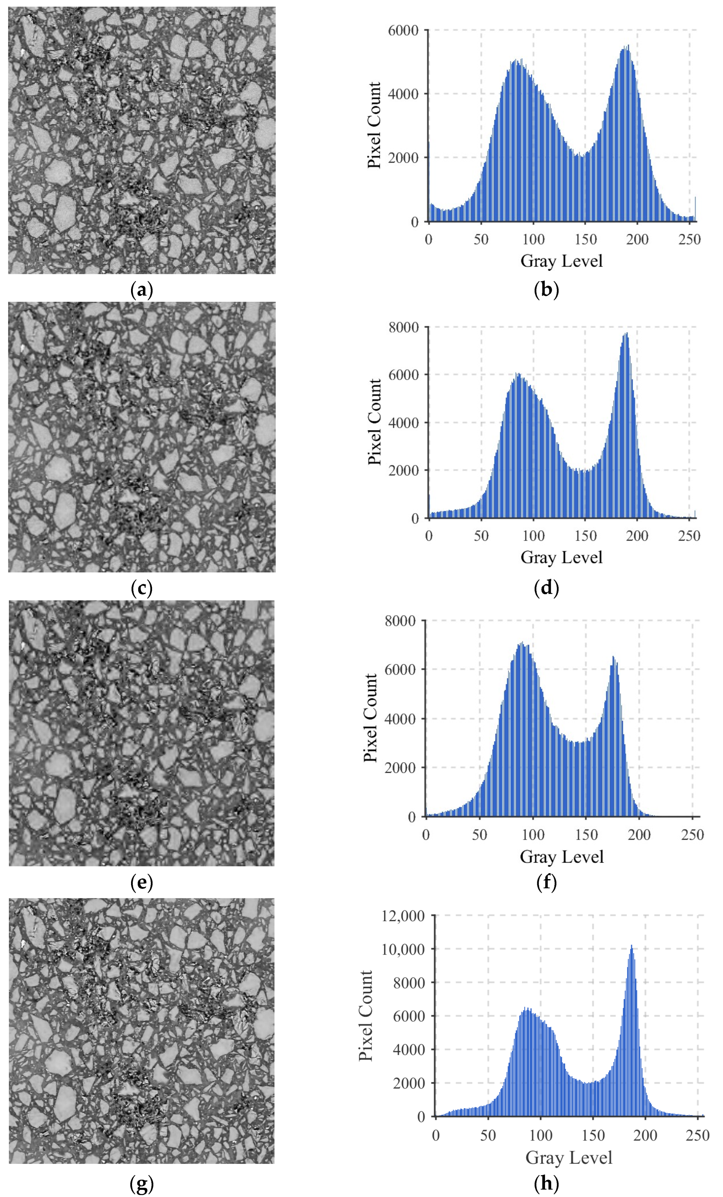
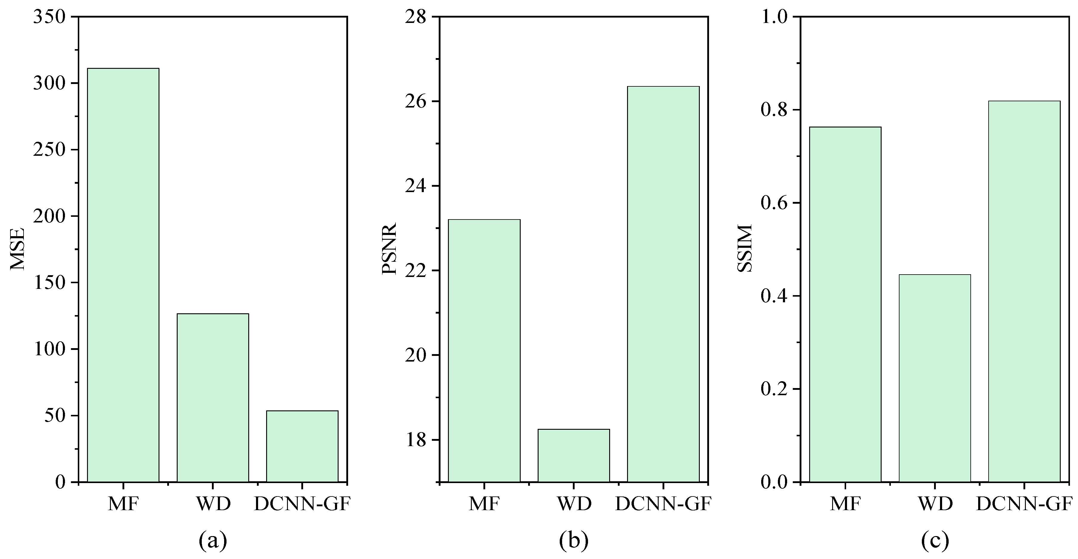
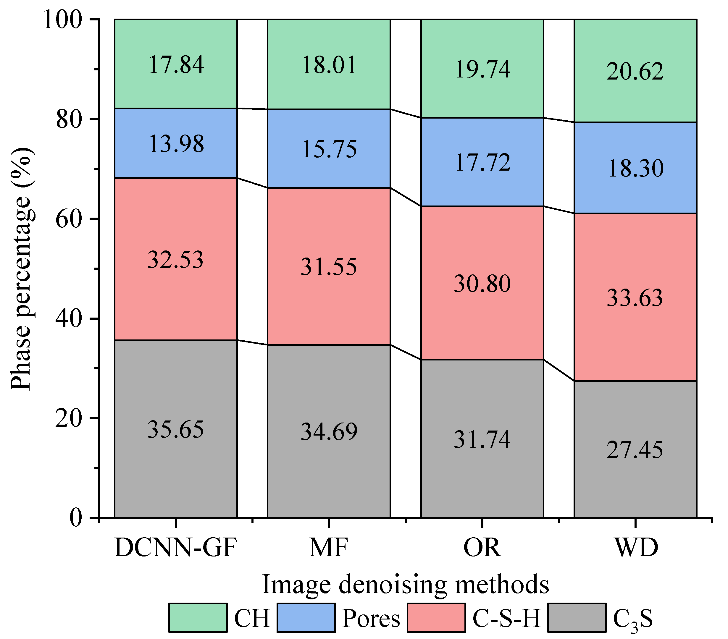
4.1.1. Influence of Image Denoising Method

Denoising prior to image segmentation is critical because noise can negatively impact the segmentation process, leading to erroneous results. This section compares results obtained with MF, WD, and DCNN-GF. Figure 5a,c,e,g display the original hydrated C₃S microstructure image, the median-filtered image, the wavelet-denoised image, and the DCNN-GF-processed image, respectively. Figure 5b,d,f, and h show the corresponding grayscale histograms of Figure 5a,c,e,g.

The quality of image processing was evaluated using mean squared error (MSE), peak signal-to-noise ratio (PSNR), and structural similarity index (SSIM). The average squared difference between pixel values of the original and processed images was evaluated using MSE, which can be calculated using Equation (10) [30].

$$P_{MSE}={\displaystyle \frac{1}{MN}}{\displaystyle \sum _{i=1}^M{\displaystyle \sum _{j=1}^N{\left[I\left(i,j\right)-K\left(i,j\right)\right]}^2}}$$

(10)

where $I$ is the original image with size of $M\times N$; $K$ is the denoised image.

The PSNR quantifies the ratio between the maximum possible signal power and the noise power, which can be mathematically represented using Equation (11) [31].

$$P_{PSNR}=10{\log }_{10}\left({\displaystyle \frac{L^2}{P_{MSE}}}\right)$$

(11)

where $P_{PSNR}$ is the PSNR; $L$ is the maximum possible pixel value.

The SSIM quantifies the similarity between two images based on luminance, contrast, and structural comparisons, which can be expressed using Equation (12) [32].

$$P_{SSIM}={\displaystyle \frac{\left(2{\mu }_x{\mu }_y+C_1\right)\left(2{\sigma }_{xy}+C_2\right)}{\left({\mu }_x^2+{\mu }_y^2+C_1\right)\left({\sigma }_x^2+{\sigma }_y^2+C_2\right)}}$$

(12)

where ${\mu }_x$ and ${\mu }_y$ are average pixel intensity of image patches $x$ and $y$, respectively; ${\sigma }_x$ and ${\sigma }_y$ are the square root of the variance of pixel intensities $x$ and $y$; ${\sigma }_{xy}$ is the covariance between pixel intensities of patches $x$ and $y$; $C_1={\left(k_{1}L\right)}^2$ and $C_2={\left(k_{2}L\right)}^2$ are stabilization constants.

The denoising performance across three methods (namely, DCNN-GF, MF, and WD) was quantitatively evaluated according to MSE, PSNR, and SSIM. The calculated values of MSE, PSNR, and SSIM for the median-filtered image, the wavelet-denoised image, and the DCNN-GF-processed image are shown in Figure 6. The results revealed significant differences in their effectiveness. The DCNN-GF achieved the best results, with an MSE of 53.52, PSNR of 26.35 dB, and SSIM of 0.8187, demonstrating its ability to minimize pixel-level errors while preserving structural fidelity. In contrast, MF yields an MSE of 311.01, PSNR of 23.20 dB, and SSIM of 0.763, indicating moderate noise suppression at the cost of blurred details, as evidenced by its higher MSE and lower SSIM compared to the DCNN-GF. Notably, WD performs the poorest, with an MSE of 126.54, PSNR of 18.25 dB, and critically low SSIM of 0.446, suggesting severe structural distortion attributed to over-aggressive thresholding that disproportionately suppresses high-frequency components essential for texture representation. The stark divergence in SSIM values—where the deep learning-based method exhibits an SSIM 83.6% higher than WD—highlights the limitations of traditional frequency-domain methods in maintaining perceptual quality compared to data-driven approaches. These results align with established findings that deep neural networks excel in predicting noise patterns and preserving edge integrity, as reflected in their balanced optimization of both pixel accuracy (MSE and PSNR) and structural coherence (SSIM) [32,33].

In stereology, the volume fraction of a phase in a three-dimensional (3D) material can be estimated from its area fraction measured in two-dimensional (2D) cross-sections, based on the Delesse principle [34]. This principle states that, for a statistically homogeneous and isotropic material, the area fraction of a phase observed in random 2D sections is equivalent to its volume fraction in 3D. Mathematically, as expressed in Equation (13), the phase percentage in this study was subsequently calculated using the same equation.

$$f_v=f_a={\displaystyle \frac{A_{phase}}{A_{total}}}$$

(13)

where $f_v$ is the volume fraction of a phase in a three-dimensional (3D) material; $f_a$ is the area fraction of a phase in a two-dimensional cross-section; $A_{phase}$ is the area of a phase in a two-dimensional cross-section; $A_{total}$ is the total area of the phase in a two-dimensional cross-section.

Figure 7 shows the quantitative phase distribution results obtained through weighted k-means clustering, which reveal significant variations depending on the pre-processing denoising methodology. DCNN-GF denoising demonstrates superior performance in preserving critical cementitious phases, maintaining the highest C₃S (35.65%) and C-S-H (32.53%) proportions among all methods. This aligns with the capability of deep neural networks to suppress noise while retaining microstructural features through learned hierarchical representations [27]. The MF shows comparable phase preservation for binder phases (C₃S: 34.69%, C-S-H: 31.55%), though with a 12.7% relative increase in pore detection compared to DCNN-GF. The inherent edge-blurring effect of MF likely contributes to this over-segmentation of porous regions. Notably, WD achieves the highest pore phase proportion (18.30%), exceeding the original image baseline by 3.3%. This indicates that pore boundary contrast is effectively enhanced by the multi-resolution characteristics of the wavelet transform. Moreover, the phase percentages of pores obtained with DCNN-GF, MF, and WD were 17.84%, 18.01%, and 20.62%, respectively. These results align closely with those reported in reference [11], where the pore percentage (C₃S paste with w/s = 0.3, hydrated for 3 days) was estimated at 21.5%. The relative deviations between the results from DCNN-GF, MF, and WD and the reference value were 17.2%, 16.23%, and 4.09%, respectively. The relative deviation obtained with WD is the lowest. This suggests that WD may be more suitable for pore network analysis compared to other image denoising methods. However, WD simultaneously yields the lowest C₃S content (27.45%), indicating potential over-smoothing of anhydrous C₃S grain features. The original image results demonstrate inherent noise-induced artifacts: (1) depressed C-S-H detection (30.80% vs. DCNN-GF’s 32.53%), and (2) exaggerated pore phase proportion (17.72% vs. DCNN-GF’s 13.98%). This underscores the necessity of appropriate denoising before microstructural quantification. A critical trade-off emerges between phase conservation and pore detection accuracy. Through the above analysis, it can be concluded that the DCNN-GF method is suitable for tasks requiring both pixel-level accuracy and high structural fidelity, such as high-precision retention of cementitious phases (e.g., C₃S, C-S-H). The WD method should be prioritized when preserving pore-edge sharpness is critical (e.g., pore parameter analysis) and global structural distortions are acceptable. The MF method is suitable for tasks that prioritize fast denoising (fastest processing speed) over detail fidelity and accept moderate blur.

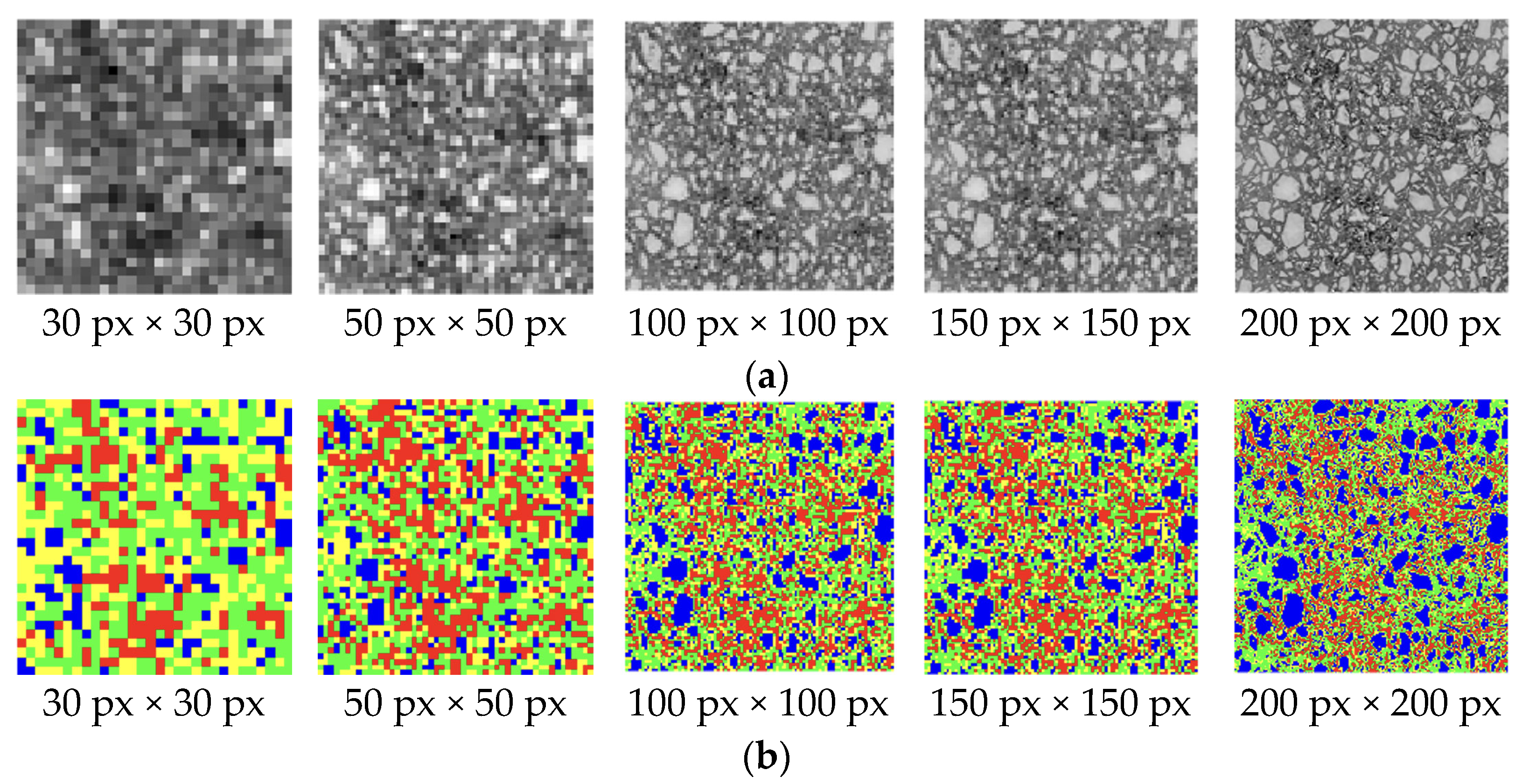
4.1.2. Influence of Image Resolution

Analyzing the impact of image resolution on phase segmentation in microstructure images is crucial for accurately characterizing material composition and properties, as it directly affects the delineation of fine-scale features and thus, the reliability of quantitative analyses. BSE images at sizes of 30 × 30, 50 × 50, 100 × 100, 150 × 150, and 200 × 200 pixels were employed for segmentation. Figure 8a,b show the original image and segmented images at different resolutions, respectively. The relative resolution was defined to characterize the influence of image resolution on segmentation, as expressed in Equation (14).

$$R_{relative}={\displaystyle \frac{{S_{image}}^2}{{S_{\max }}^2}}$$

(14)

where $R_{relative}$ is the relative resolution; $S_{image}$ is the image size, in pixels; $S_{\max }$ is the size of the largest image in the database, in pixels.

Intra-region variance (IRV) is a metric utilized in image segmentation to evaluate intra-region homogeneity, as expressed in Equation (15) [30]. It calculates the variance of gray value within a region. A lower IRV indicates higher consistency within a region, implying better segmentation or clustering performance.

$$p_m={\displaystyle \frac{1}{n_{\mathrm{intra}}}}{\displaystyle \sum _{j=1}^{n_{\mathrm{intra}}}{\left(x_j-{\mu }_{\mathrm{intra}}\right)}^2}$$

(15)

where $p_m$ is the mean intra-region variance; $n_{\mathrm{intra}}$ is the total number of pixels within the region; $x_j$ is the gray value of the $j$-th pixel in the region; and ${\mu }_{\mathrm{intra}}$ is the mean gray value of all pixels in the region.

Boundary strength (BS) measures the average intensity difference between neighboring pixels across the boundary of a region, as expressed in Equation (16). Higher values indicate stronger edges or clearer boundaries.

$${\displaystyle \frac{1}{N_b}}{\displaystyle \sum _{i=1}^{N_b}\left|I_i^{in}-I_i^{out}\right|}$$

(16)

where $N_b$ is the number of boundary pixels; $I_i^{in}$ is the intensity of the $i$-th boundary pixel inside the region; $I_i^{out}$ is the intensity of the $i$-th boundary pixel outside the region.

Figure 9a shows the relationship between IRV and relative resolution for different phases. During the low-resolution phase (0.0014–0.035), blurred C₃S particle boundaries lead algorithms to misinterpret single angular particles (5–50 μm) as multiple regions, artificially inflating variance (134.6 → 75.96). During mid-resolution phase (0.035–0.39), enhanced boundary clarity at moderate resolutions reduces segmentation errors, minimizing variance (trough at 75.96). During high-resolution phase (0.39–1.0), larger images expose microstructural noise (e.g., pore-C₃S coupling), causing inconsistent edge detection and variance resurgence (75.96 → 129.4). The pore phase has the highest IRV. This phenomenon could be ascribed to a multi-scale network. As image resolution increases (relative resolution: 0.0014 → 1.0), additional pore sub-structures are progressively identified, leading to continuous variance accumulation. Whereas the microstructures of C-S-H stabilized beyond a specific resolution (i.e., 0.25) due to self-similar aggregation of fractal gels. The stabilization of the IRV of CH can be explained by crystal size saturation. CH crystals are hexagonal platelets with typical dimensions of 1–10 μm in diameter and 0.1–1 μm in thickness. At resolutions >0.25, CH crystals are fully resolved, and further magnification only repeats observations of the same structural hierarchy.

Figure 9b shows the relationship between the BS and relative resolution with respect to different phases. The BS of four phases (unhydrated C₃S, C-S-H, CH, and pores) exhibits distinct trends with increasing relative resolution (0.0014 to 1.0). Unhydrated C₃S reflects optimal boundary clarity at intermediate resolutions (0.25–0.56), likely due to balanced detection of angular particle edges (5–50 μm) and suppressed noise. For C-S-H, the BS gradually increases to 223.6 (resolution 0.32), followed by fluctuations (±5%), which indicates that moderate resolutions best resolve gel-pore interfaces. For CH, the BS reaches a maximum of 228.3 (resolution 0.19), then oscillates downward (±8%). The value of BS for CH indicates orientation-dependent edge detection limits for hexagonal platelets (1–10 μm), with stacking complexity reducing boundary consistency at high resolutions. The values of BS for pores peak at 258.2 (resolution 0.14), then decline linearly (R² = 0.94) to 213.4. The results indicate challenges in maintaining boundary accuracy for multiscale fractal networks.

4.1.3. Influence of Cluster Number

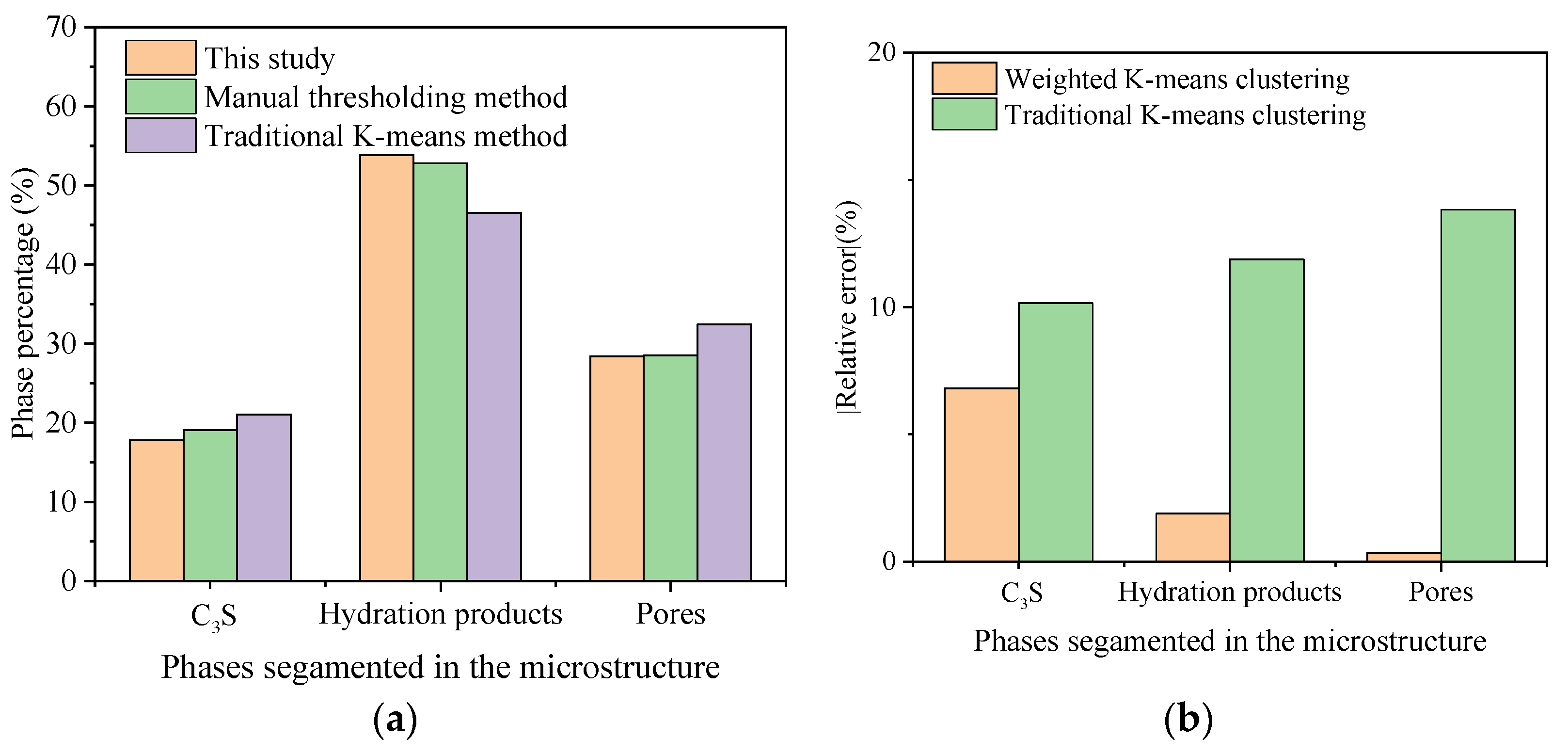
Figure 10 shows the segmented images obtained with different cluster numbers ($K$ = 2, 3, 4). The coefficient of variation ($C_v$), defined as the ratio of the standard deviation to the mean [Equation (17)], was used to quantify segmentation consistency. $C_v$ values for C₃S percentage obtained with $K=2$, $K=3$ and $K=4$ were calculated as 0.66%, 2.08%, and 4.9%, respectively. These results demonstrate a clear trend: higher cluster numbers lead to greater segmentation instability ($r$ increased by 6.4× from $K=2$ to $K=4$), likely due to over-segmentation in low-contrast regions.

$$C_v={\displaystyle \frac{s}{\overline{x}}}\times 100\%$$

(17)

where $r$ represents the coefficient of variation; $s$ represents the standard deviation of the dataset; and $\overline{x}$ represents the mean of the dataset.

Figure 11 shows the microstructure of unhydrated C₃S obtained with varying cluster numbers. The edges of C₃S particles were clearly defined, indicating that weighted K-means clustering could effectively distinguish unhydrated C₃S particles from other phases. The percentage of unhydrated C₃S slightly decreased as the K-value increased. The Silhouette coefficient was utilized to evaluate clustering quality. This metric combines cohesion and separation measures in clustering, quantifying both: (1) the similarity between an object and others within its cluster, (2) the dissimilarity between that object and objects in neighboring clusters. The calculation formula for the silhouette coefficient is given in Equation (18), and the average silhouette coefficient is calculated using Equation (19).

$$s\left(i\right)={\displaystyle \frac{b\left(i\right)-a\left(i\right)}{\max \left\{a\left(i\right)-b\left(i\right)\right\}}}$$

(18)

$$S={\displaystyle \frac{1}{N}}\cdot {\displaystyle \sum s\left(i\right)}$$

(19)

where $s\left(i\right)$ represents the silhouette coefficient for sample $i$; $b\left(i\right)$ is the average nearest-cluster distance for sample $i$; $a\left(i\right)$ is the average intra-cluster distance for sample $i$; $S$ is the average silhouette coefficient, representing the average of $s\left(i\right)$ for all samples; $N$ is the total number of samples in the dataset.

Figure 12a–c show the silhouette coefficients for each data point in microstructure images with cluster numbers of 2, 3, and 4, respectively. The average silhouette values for cluster numbers 2, 3, and 4 were 0.8427, 0.7440, and 0.7018, respectively. These values fall within the range of 0.7–1, indicating relatively good overall clustering quality across all three cases. In Figure 12a, a clear separation between the two main clusters is observed. However, the presence of a few data points in Cluster 1 (other phases) with silhouette scores below 0 suggests potential microstructural impurities. Similar patterns were observed in Figure 12b,c. Furthermore, the progressive decrease in average silhouette values from 0.8427 ($K=2$) to 0.7018 ($K=4$) demonstrates diminished clustering quality with increasing cluster numbers.

4.2. Validation

The approach proposed in this study was compared with that reported in Reference [35]. In the reference work, hydrated C₃S images were segmented using a grayscale-thresholding method dependent on manually selected threshold values. The BSE image of a 7-day hydrated C₃S specimen was obtained from a public database [36], with a w/s ratio of 0.5. Specimen preparation procedures are detailed in Reference [35]. The thresholding algorithm was implemented using Python 3.11 (publicly available code [37]). As shown in Figure 13a, the area of the original image and pixel size are 2.41 mm² and 42.16 nm per px, respectively. The original microstructure underwent denoising using the Non-Local Means algorithm [38] for threshold-based segmentation [35]. In contrast, our method employed DCNN-GF for denoising, resulting in distinct phase segmentation (Figure 13b). The phase percentages obtained in this study were compared with those from the grayscale-thresholding method, as shown in Figure 14a.

As shown in Figure 14a, the phase percentages for C₃S, hydration products, and pores calculated by the weighted K-means clustering method are 17.8%, 53.8%, and 28.4%, respectively. The corresponding values obtained in Kleiner et al. [35] are 19.1%, 52.8%, and 28.5%. The relative errors of results obtained with the weighted K-means clustering method are −6.81%, 1.89%, and −0.35%, respectively. These errors indicate close agreement between the proposed method and the reference. Despite fundamentally different technical approaches—DCNN-GF combined with K-means clustering in this study versus non-local means (NLM) denoising with grayscale thresholding in Kleiner et al. [35]—the phase quantification results on identical samples exhibit remarkable consistency (hydrates: relative error < 2%, porosity: relative error < 0.4%). This agreement validates the efficacy of the proposed method, demonstrating that: (1) DCNN-GF achieves noise suppression and edge preservation comparable to NLM; (2) Weighted K-means clustering, through integration of textural-spatial features, effectively replaces manual thresholding for precise phase segmentation while mitigating operator-dependent bias. In Figure 14a, the phase percentages for C₃S, hydration products, and pores calculated by the traditional K-means clustering method are 21.04%, 46.53%, and 32.44%, respectively. The relative errors of results obtained with the traditional K-means clustering method are 10.16%, −11.87%, and 13.83%, respectively. The absolute relative errors of C₃S, hydration products, and pores obtained by traditional K-means clustering are 1.5 times, 6.3 times, and 39.5 times those of the weighted K-means clustering method, respectively (see Figure 14b). These results demonstrate that incorporating weighted features into traditional K-Means clustering significantly improves the accuracy of phase segmentation.

4.3. Applications

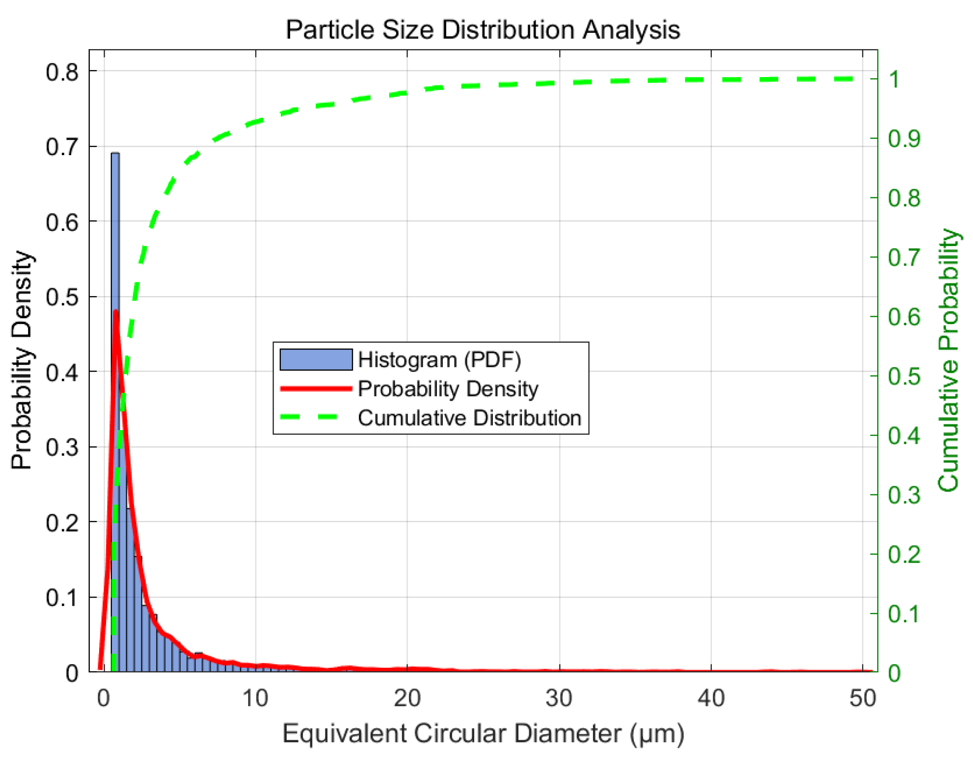
4.3.1. Estimating Particle Size Distribution During the Hydration

The particle size distribution of 28-day hydrated C₃S (w/s ratio = 0.4) was determined through analysis of BSE images. Figure 15a displays the original BSE micrograph of the C₃S microstructure, which underwent segmentation via the weighted K-means clustering algorithm. The resultant binary image identifying C₃S particles is presented in Figure 15b, with the original image resolution being 0.5802 μm/px. Equivalent circular diameter (ECD), mathematically defined in Equation (20), was employed to characterize irregular C₃S particles by representing them as geometrically idealized circles. The values for mean diameter, median diameter, D₁₀, and D₉₀ obtained from analysis were 3.28, 1.46, 0.65, and 7.55 μm, respectively. The curves of probability density, histogram, and cumulative distribution obtained from the analysis are shown in Figure 16.

$$D_{\mathrm{eq}}=2\sqrt{{\displaystyle \frac{A}{\pi }}}$$

(20)

where $D_{\mathrm{eq}}$ is the equivalent circular diameter, in μm; $A$ is the actual area of a C₃S particle, in μm.

In Figure 16, the particle size distribution of C₃S after 28 days of hydration exhibits a polydisperse and right-skewed profile. Quantitative analysis reveals a median diameter (D₅₀) of 1.46 μm, with 10% of particles below 0.65 μm (D₁₀) and 90% below 7.55 μm (D₉₀). The significant disparity between the arithmetic mean diameter (3.28 μm) and D₅₀ highlights the asymmetric distribution, where a population of larger particles (>7 μm) coexists with a dominant fraction of submicron to low-micron scale C₃S grains.

4.3.2. Distribution of CH

Figure 17a shows the BSE image of C₃S paste with a w/s ratio of 0.3, hydrated for 28 days. The original BSE image has a pixel resolution of 1.56 μm/pixel and dimensions of 800 × 800 pixels. Figure 17b shows the segmented image, which clearly represents CH (green-colored), C-S-H (red-colored), C₃S (blue-colored), and pores (black-colored). In the figure, CH grew around several centers and precipitated as large deposits rather than being randomly distributed in the pore space. A similar phenomenon has also been reported by Kjellsen and Justnes [39].

To determine the centers where CH grew around in the image, a Monte Carlo approach was developed. Specifically, for each simulation iteration, a circle center was randomly sampled within the image boundaries, ensuring that the entire circle (with a predefined radius) remained within the image domain. A binary mask was then created to identify pixels within the circle, and the sum of pixel values within this mask was computed. This process was repeated for a large number of iterations (e.g., 10,000), and the circles with the highest pixel value sums were selected as the optimal candidates. This method ensures unbiased sampling of circle positions while maximizing the relevance of the selected circles to the underlying image features. The full code repository is available at https://zenodo.org/record/15310678 (DOI: 10.5281/zenodo.15310678) (accessed on 30 April 2025). The simulations were performed using MATLAB R2024b (64-bit; Windows x64, released in 2024; MathWorks, Inc., Natick, MA, USA) under an academic license provided by Hohai University. The results obtained are shown in Figure 18.

The Clark–Evans index (R) is a spatial statistic used to quantify whether a set of points in a two-dimensional space exhibits clustering, randomness, or uniformity. It compares the observed mean nearest-neighbor distance to the expected distance under complete spatial randomness (CSR), as expressed in Equation (21) [40].

$$R={\displaystyle \frac{{\overline{r}}_{\mathrm{obs}}}{{\overline{r}}_{\exp }}}$$

(21)

where ${\overline{r}}_{\mathrm{obs}}$ is the observed mean nearest-neighbor distance across all points; ${\overline{r}}_{\exp }$ is the expected mean nearest-neighbor distance under CSR. Points follow a random distribution if R = 1, exhibit clustering if R < 1, and show uniformity if R > 1.

The Clark–Evans index for red cycles in C₃S paste (see Figure 18) was calculated as 0.426, which is significantly less than 1, indicating a strongly aggregated distribution pattern at the studied scale. This result suggests that CH clusters are non-randomly distributed with a high probability of neighboring points. The obtained Clark–Evans index value also implies that the observed aggregation cannot be explained by a Poisson random process. In C₃S hydration, the rapid dissolution of C₃S releases Ca²⁺ and OH⁻ ions at a high rate, creating localized regions of extreme supersaturation. This promotes non-classical nucleation pathways, such as particle aggregation or multi-step nucleation via metastable precursor phases (e.g., amorphous calcium silicate hydrates or ion clusters). These precursors act as templates for CH nucleation, leading to clustered growth rather than random precipitation. In contrast, Portland cement systems contain pozzolanic phases (e.g., fly ash, slag) or slower-reacting phases that buffer ion concentrations, reducing localized supersaturation and favoring classical nucleation with spatially random CH precipitation.

Existing studies in concrete systems have identified CH accumulation within the interfacial transition zone, where the porosity near aggregate surfaces reaches 1.2–2.5 times that of the bulk paste [41]. By analogy, the CH-rich regions formed around growth centers probably exhibit higher porosity compared to adjacent phases, potentially creating percolation pathways for sulfate ingress. Furthermore, the calcium carbonate formed through carbonation induces expansion stress within CH-rich regions, which cannot be uniformly released due to localized pore structure heterogeneity. This stress concentration probably initiates microcracks, compromising material density and establishing interconnected carbonation pathways.

The influence of the Monte Carlo simulation counts on the Clark–Evans index was analyzed. The calculated results are shown in Figure 19a. In the figure, the Clark–Evans index exhibits an exponential decay pattern (R² ≈ 0.95), decreasing from 0.98 at 1000 iterations to 0.15 at 100,000 iterations. When the iteration count exceeds 30,000, the index stabilizes at 0.15. Furthermore, the influence of the predefined radius of the circle center was also analyzed. The calculated results are shown in Figure 19b. In the figure, all Clark–Evans indices remain significantly below the random distribution threshold (R = 1), confirming strong clustering tendencies across all tested radii. The Clark–Evans index values decrease with an increasing predefined radius, stabilizing around 0.14 when the radius ≥ 25 px.

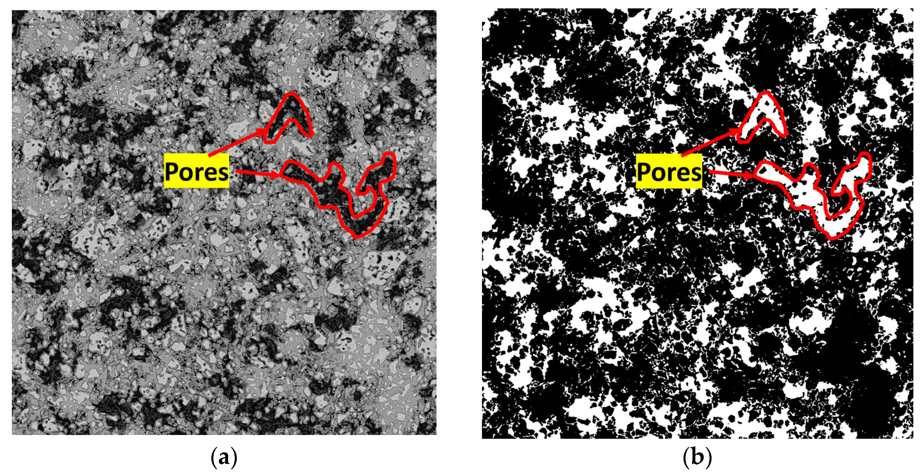
4.3.3. Pore Parameters

Figure 20a shows the original BSE image of C₃S paste with a w/s ratio of 0.5 at 14 days, adapted from a dataset [36]. The image dimensions are 5931 × 5931 pixels (width × height), with a pixel resolution of 42.16 nm/pixel. The original image was first denoised using the WD method and subsequently segmented using the weighted K-means clustering. The segmentation results of the pores (white color) are shown in Figure 20b. The porosity and pore connectivity of the hydrated C₃S paste were quantitatively evaluated through digital image analysis. Porosity ($\varphi$) was determined as the volumetric fraction of pore space using the binary image analysis, as expressed in Equation (22).

$$\varphi ={\displaystyle \frac{{\displaystyle {\sum }_{i,j}{I}_{\mathrm{pore}}\left(i,j\right)}}{N_{\mathrm{total}}}}$$

(22)

where $I_{\mathrm{pore}}\left(i,j\right)$ is the binary matrix; $N_{\mathrm{total}}$ is the total pixel count. $I_{\mathrm{pore}}\left(i,j\right)$ is 0 for solid phases, and 1 is for pores.

Pore connectivity quantifies the extent to which void spaces within a porous medium form continuous pathways for fluid flow, directly influencing permeability and mass transport efficiency. This property can be mathematically expressed by Equation (23).

$$p={\displaystyle \frac{S_{\mathrm{P}\text{-}\mathrm{connected}}}{S_{\mathrm{P}\text{-}\mathrm{total}}}}\times 100\%$$

(23)

where $p$ is the pore connectivity; $S_{\mathrm{P}\text{-}\mathrm{connected}}$ is the area of connected pores, in m³; $S_{\mathrm{P}\text{-}\mathrm{total}}$ is the total area of pores, in m³. $S_{\mathrm{P}\text{-}\mathrm{connected}}$ is determined using a binary image processing method [42].

The value for porosity is estimated as 0.2596 lies within the typical range ($\varphi$ = 20–30%) for w/s = 0.5 systems at 14 days [43], reflecting continuous hydration product formation while retaining interconnected capillary pores. For the studied material, the pore connectivity was determined as 0.6648—a magnitude comparable to cement systems at an equivalent water-to-cement ratio (w/c = 0.45) [44], suggesting analogous pore-structure evolution pathways.

5. Extensions of Proposed Method

The extension of the weighted K-means framework to multi-phase cement systems necessitates addressing phase complexity and feature overlap. In Portland cement systems, ettringite formed by tricalcium aluminate (C₃A)-sulfate reactions shares grayscale similarities with C-S-H in BSE images. To resolve this challenge, the EDS-derived Ca/Al/Si contents will be integrated as additional clustering weights in the proposed method, achieving improvement in phase differentiation accuracy compared to the original weighted K-means clustering method. By segmenting BSE images into distinct phases (e.g., unhydrated clinker, C-S-H, and pores), critical microstructure features can be identified. These features, such as pore size distribution, pore connectivity, and hydration product distribution, can be correlated with durability mechanisms (e.g., chloride ingress and carbonation). Thus, the proposed method will provide a foundational basis for durability modeling.

6. Limitations of This Study

The images used in Section 4.1.2 were generated through digital resampling with bicubic interpolation (implemented using the imresize function in MATLAB R2024b) to emulate scale-dependent microstructural evolution. Although this approach enables controlled parametric studies of resolution effects, it inherently incorporates algorithmic compensation for feature boundaries rather than capturing true physical resolution variations. This is the first limitation of this study. In future work, the influence of the actual physical resolution of images on segmentation will be investigated.

The proposed model was not benchmarked against state-of-the-art deep learning models (e.g., U-Net variants) due to the scarcity of labeled microstructure data, which is the second limitation of this study. Future work will address this gap through semi-automated annotation frameworks and hybrid architectures that integrate deep learning to enhance generalizability across heterogeneous cement systems.

7. Conclusions

A weighted K-means clustering approach considering intensity gradients, texture variations, and spatial coordinates features was developed to quantitatively analyze the microstructure of hydrated C₃S. The conclusions can be summarized as follows:

(1)

The superior performance of DCNN-GF (MSE: 53.52, PSNR: 26.35 dB, SSIM: 0.8187) stems from its hybrid architecture. DCNN’s multi-scale feature extraction preserves phase boundaries, while GF adaptively smooths high-frequency noise without blurring textural details. This dual mechanism makes DCNN-GF uniquely suited for hydration kinetics studies requiring precise phase quantification (e.g., residual C₃S evolution and C-S-H gel). In contrast, WD prioritizes pore network analysis but results in partial loss of solid phase information. These results establish a selection criterion: DCNN-GF for reaction front analysis, as well as WD for durability-related pore network modeling;

(2)

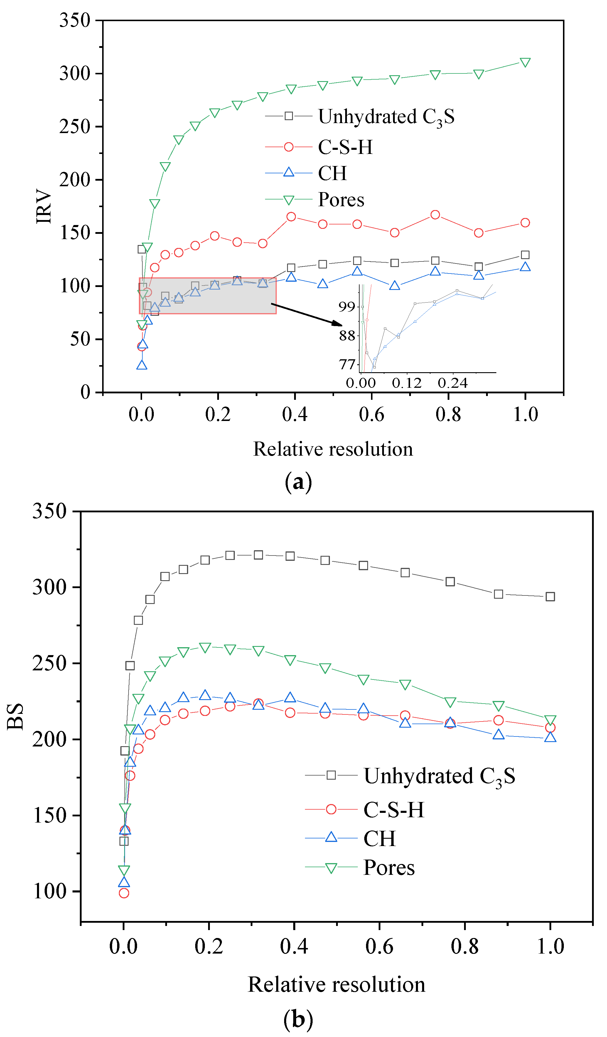
For IRV, low resolutions cause particle misidentification, mid resolutions optimize boundary clarity, while high resolutions introduce microstructural noise. Pores exhibit the highest IRV due to multi-scale networks. C-S-H stabilizes above 0.25 resolution through fractal aggregation, while CH stabilizes via crystal saturation. For BS, optimal boundary detection occurs at medium image relative resolutions (0.14–0.56), with C₃S peaking at 0.25–0.56, C-S-H at 0.32, and CH at 0.19. Pores show a linear BS decline due to fractal complexity;

(3)

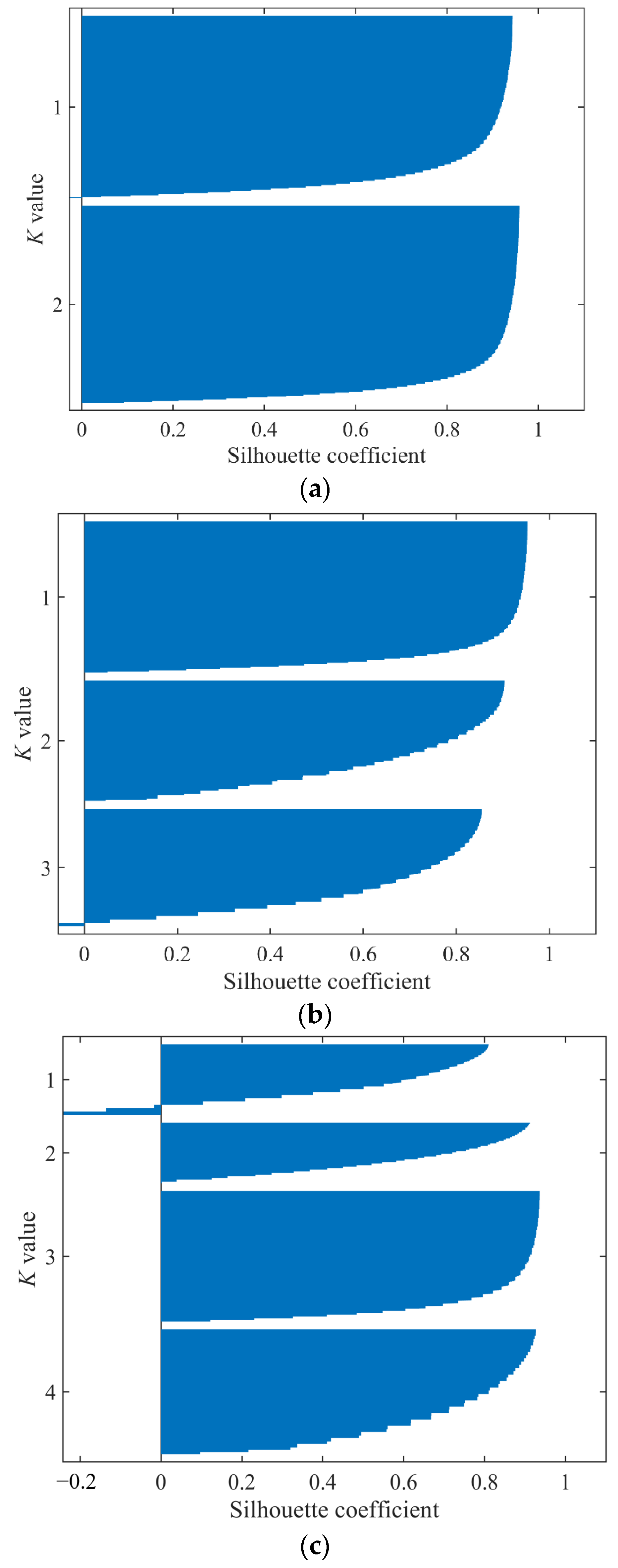
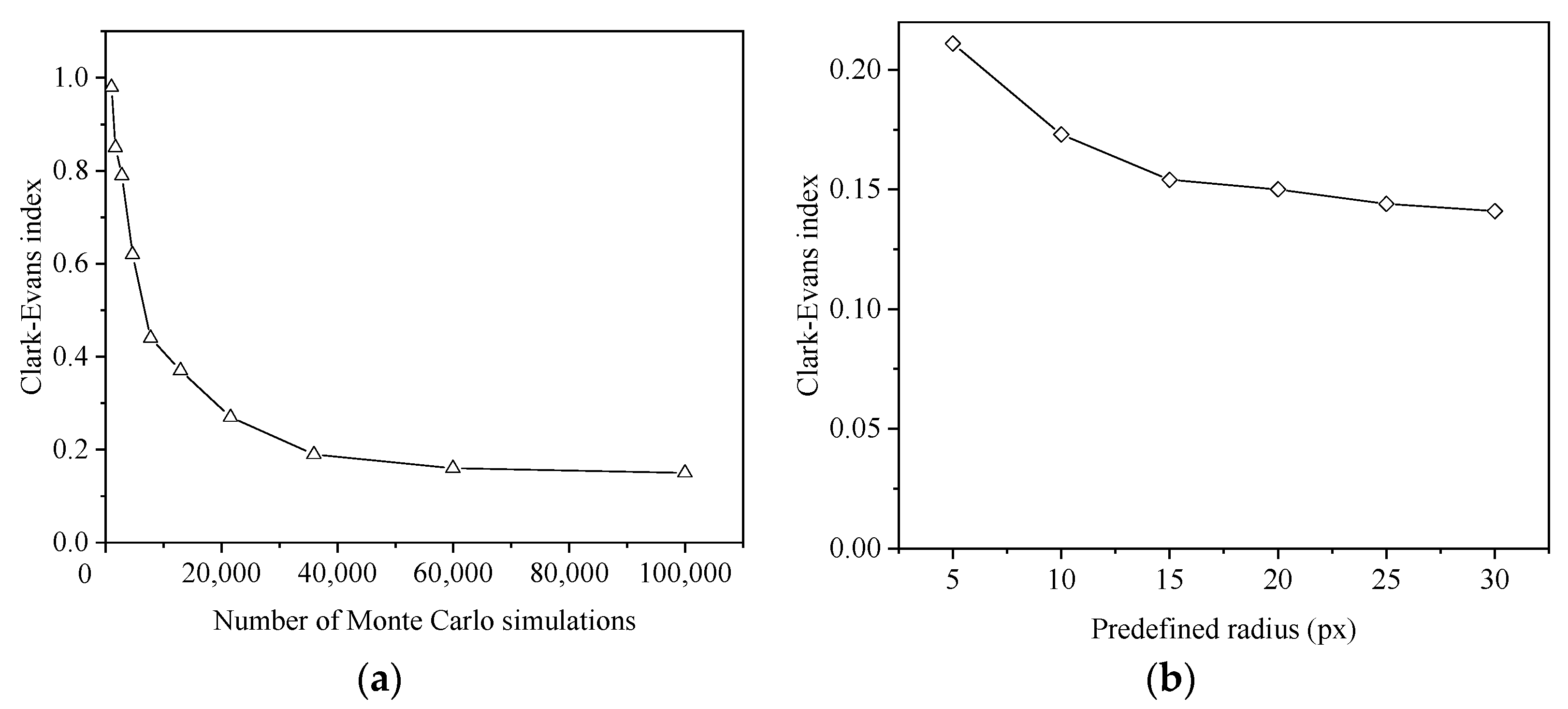
Silhouette analysis (average: 0.70–0.84) validates robust clustering when the number of clusters is 2–4. The Clark–Evans index of CH (0.426) reveals non-classical nucleation mechanisms in C₃S hydration. Unlike Portland cement systems, where CH randomly precipitates within pore spaces, C₃S-derived CH forms distinct nucleation centers within the microstructure.

References

1. Hache, E.; Simoën, M.; Seck, G.S.; Bonnet, C.; Jabberi, A.; Carcanague, S. The impact of future power generation on cement demand: An international and regional assessment based on climate scenarios. Int. Econ. 2020, 163, 114–133. [Google Scholar] [CrossRef]
2. Taylor, H.F.W. Cement Chemistry, 2nd ed.; Thomas Telford: London, UK, 1997. [Google Scholar]
3. Wu, S.; Wang, X.; Shen, D.; Sun, K.; Zhu, J. Simulation analysis on hydration kinetics and microstructure development of tricalcium silicate considering dissolution mechanisms. Constr. Build. Mater. 2020, 249, 118535. [Google Scholar] [CrossRef]
4. Wang, X.; Shen, D.; Tao, S.; Liu, R.; Wu, S. Estimation of chloride diffusivity in hydrated tricalcium silicate using a hydration-diffusion integrated method. J. Wuhan Univ. Technol.-Mater. Sci. Ed. 2025, 40, 49–64. [Google Scholar] [CrossRef]
5. Camerini, R.; Poggi, G.; Ridi, F.; Baglioni, P. The kinetic of calcium silicate hydrate formation from silica and calcium hydroxide nanoparticles. J. Colloid Interface Sci. 2022, 605, 33–43. [Google Scholar] [CrossRef]
6. Liu, X.; Feng, P.; Cai, Y.; Yu, X.; Liu, Q. Carbonation behaviors of calcium silicate hydrate (C-S-H): Effects of aluminum. Constr. Build. Mater. 2022, 325, 126825. [Google Scholar] [CrossRef]
7. Prabhu, A.; Dolado, J.S.; Koenders, E.A.B.; Zarzuela, R.; Mosquera, M.J.; Garcia-Lodeiro, I.; Blanco-Varela, M.T. A patchy particle model for C-S-H formation. Cem. Concr. Res. 2022, 152, 106658. [Google Scholar] [CrossRef]
8. Kurdowski, W. Cement and Concrete Chemistry, 1st ed.; Springer: Dordrecht, The Netherlands, 2014. [Google Scholar]
9. Salah Uddin, K.M.; Izadifar, M.; Ukrainczyk, N.; Koenders, E.; Middendorf, B. Dissolution of portlandite in pure water: Part 1 molecular dynamics (MD) approach. Materials 2022, 15, 1404. [Google Scholar] [CrossRef]
10. Izadifar, M.; Ukrainczyk, N.; Salah Uddin, K.M.; Middendorf, B.; Koenders, E. Dissolution of portlandite in pure water: Part 2 atomistic kinetic Monte Carlo (KMC) approach. Materials 2022, 15, 1442. [Google Scholar] [CrossRef]
11. Shen, D.; Wang, X. Simulation on Hydration of Tricalcium Silicate in Cement Clinker, 1st ed.; Springer: Singapore, 2023. [Google Scholar]
12. Taylor, H.F.W.; Mohan, K.; Moir, G.K. Analytical study of pure and extended portland cement pastes: I, pure Portland cement pastes. J. Am. Ceram. Soc. 1985, 68, 680–685. [Google Scholar] [CrossRef]
13. Bentz, D.P.; Stutzman, P.E.; Haecker, C.; Remond, S. SEM/X-ray imaging of cement-based materials. In Proceedings of the 7th Euroseminar on Microscopy Applied to building Materials, Delft, Holland, 29 June–2 July 1999; pp. 457–466. [Google Scholar]
14. Wong, H.S.; Head, M.K.; Buenfeld, N.R. Pore segmentation of cement-based materials from backscattered electron images. Cem. Concr. Res. 2006, 36, 1083–1090. [Google Scholar] [CrossRef]
15. Gao, Y.; De Schutter, G.; Ye, G.; Huang, H.; Tan, Z.; Wu, K. Characterization of ITZ in ternary blended cementitious composites: Experiment and simulation. Constr. Build. Mater. 2013, 41, 742–750. [Google Scholar] [CrossRef]
16. Scrivener, K.L. Backscattered electron imaging of cementitious microstructures: Understanding and quantification. Cem. Concr. Compos. 2004, 26, 935–945. [Google Scholar] [CrossRef]
17. Chen, L.; Shan, W.; Liu, P. Identification of concrete aggregates using K-means clustering and level set method. Structures 2021, 34, 2069–2076. [Google Scholar] [CrossRef]
18. Li, L.; Yang, J.; Shen, X. Measuring the hydration product proportion in composite cement paste by using quantitative BSE-EDS image analysis: A comparative study. Measurement 2022, 199, 111290. [Google Scholar] [CrossRef]
19. Yu, Y.; Geng, G. Deep learning methods for phase segmentation in backscattered electron images of cement paste and SCM-blended systems. Cem. Concr. Compos. 2025, 155, 105810. [Google Scholar] [CrossRef]
20. Sheiati, S.; Nguyen, H.; Kinnunen, P.; Ranjbar, N. Cementitious phase quantification using deep learning. Cem. Concr. Res. 2023, 172, 107231. [Google Scholar] [CrossRef]
21. Ma, Y.; Qian, H.; Zou, D.; Zhou, A.; Liu, T.; Li, Y. Resolution enhancement of cementitious microstructure images and phases quantification using deep learning. Constr. Build. Mater. 2025, 461, 139909. [Google Scholar] [CrossRef]
22. Abras, G.N.; Ballarin, V.L. A weighted K-means algorithm applied to brain tissue classification. J. Comput. Sci. Technol. 2005, 5, 121–126. [Google Scholar]
23. Costoya Fernández, M.M. Effect of Particle Size on the Hydration Kinetics and Microstructural Development of Tricalcium Silicate. Ph.D. Thesis, EPFL, Lausanne, Switzerland, 2008. [Google Scholar]
24. Young, J.F.; Hansen, W. Volume relationships for C-S-H formation based on hydration stoichiometries. MRS Online Proc. Libr. 1986, 85, 313. [Google Scholar] [CrossRef]
25. Wei, D.; Rajashekar, U.; Bovik, A.C. 3.4-Wavelet denoising for image enhancement. In Handbook of Image and Video Processing, 2nd ed.; Bovik, A.L., Ed.; Academic Press: Burlington, VT, USA, 2005; pp. 157–165. [Google Scholar]
26. Dinç, İ.; Dinç, S.; Sigdel, M.; Sigdel, M.S.; Aygün, R.S.; Pusey, M.L. Chapter 12-DT-Binarize: A decision tree based binarization for protein crystal images. In Emerging Trends in Image Processing, Computer Vision and Pattern Recognition; Deligiannidis, L., Arabnia, H.R., Eds.; Morgan Kaufmann: Boston, MA, USA, 2015; pp. 183–199. [Google Scholar]
27. He, K.; Sun, J.; Tang, X. Guided image filtering. IEEE Trans. Pattern Anal. Mach. Intell. 2013, 35, 1397–1409. [Google Scholar] [CrossRef]
28. MacQueen, J.B.; Le Cam, L.M.; Neyman, J. Some methods for classification and analysis of multivariate observations. In Proceedings of the Fifth Berkeley Symposium on Mathematical Statistics and Probability, Berkeley, CA, USA, 21 June–18 July 1965 and 27 December 1965–7 January 1966; University of California Press: Berkeley, CA, USA, 1967; pp. 281–297. [Google Scholar]
29. Poynton, C. Digital Video and HDTV: Algorithms and Interfaces, 1st ed.; Morgan Kaufmann: San Francisco, CA, USA, 2012. [Google Scholar]
30. Gonzalez, R.C.; Woods, R.E. Digital Image Processing, 1st ed.; Pearson: Essex, UK, 2018. [Google Scholar]
31. Horé, A.; Ziou, D. Image quality metrics: PSNR vs. SSIM. In Proceedings of the 2010 20th International Conference on Pattern Recognition, Istanbul, Turkey, 23–26 August 2010; pp. 2366–2369. [Google Scholar]
32. Zhou, W.; Bovik, A.C.; Sheikh, H.R.; Simoncelli, E.P. Image quality assessment: From error visibility to structural similarity. IEEE Trans. Image Process. 2004, 13, 600–612. [Google Scholar] [CrossRef] [PubMed]
33. Zhang, K.; Zuo, W.; Chen, Y.; Meng, D.; Zhang, L. Beyond a Gaussian denoiser: Residual learning of deep CNN for image denoising. IEEE Trans. Image Process. 2017, 26, 3142–3155. [Google Scholar] [CrossRef]
34. Oleschko, K. Delesse principle and statistical fractal sets: 1. Dimensional equivalents. Soil Tillage Res. 1998, 49, 255–266. [Google Scholar] [CrossRef]
35. Kleiner, F.; Becker, F.; Rößler, C.; Ludwig, H.-M. A Python tool to determine the thickness of the hydrate layer around clinker grains using SEM-BSE images. J. Microsc. 2024, 294, 146–154. [Google Scholar] [CrossRef] [PubMed]
36. Kleiner, F. Large SEM-BSE Images of Hydrated Alite of Ages from 1 Day up to 1 Year. Zenodo. Available online: https://zenodo.org/records/8210797 (accessed on 6 July 2023).
37. Kleiner, F. ELM/Measure_Hydrate_Layer: Release for Revision 1. Zenodo. Available online: https://zenodo.org/records/10659663 (accessed on 14 February 2024).
38. Buades, A.; Coll, B.; Morel, J.M. Non-local means denoising. Image Process. Line 2011, 1, 208–212. [Google Scholar] [CrossRef]
39. Kjellsen, K.O.; Justnes, H. Revisiting the microstructure of hydrated tricalcium silicate––A comparison to Portland cement. Cem. Concr. Compos. 2004, 26, 947–956. [Google Scholar] [CrossRef]
40. Petrere, M. The variance of the index (R) of aggregation of Clark and Evans. Oecologia 1985, 68, 158–159. [Google Scholar] [CrossRef]
41. Gao, X.; Liu, Q.-F.; Cai, Y.; Tong, L.-Y.; Peng, Z.; Xiong, Q.X.; De Schutter, G. A new model for investigating the formation of interfacial transition zone in cement-based materials. Cem. Concr. Res. 2025, 187, 107675. [Google Scholar] [CrossRef]
42. Jain, R.; Kasturi, R.; Schunck, B.G. Machine Vision, 1st ed.; McGraw-Hill: London, UK, 1995. [Google Scholar]
43. Termkhajornkit, P.; Vu, Q.H.; Barbarulo, R.; Daronnat, S.; Chanvillard, G. Dependence of compressive strength on phase assemblage in cement pastes: Beyond gel–space ratio—Experimental evidence and micromechanical modeling. Cem. Concr. Res. 2014, 56, 1–11. [Google Scholar] [CrossRef]
44. Liu, C.; Zhang, M.; Fang, G.; Bai, Y.; Zhang, Y. Modelling of capillary pore structure evolution in Portland cement pastes based on irregular-shaped cement particles. In Proceedings of the 6th International Conference on Durability of Concrete Structures, Leeds, UK, 18–20 July 2018; pp. 771–780. [Google Scholar]
Figure 1. XRD pattern of synthesized C3S. The red markers indicate the positions of numerical values.
Buildings 15 01699 g001
Figure 2. Preparing C3S particles: (a) C3S particles sieved using a 300-mesh sieve; (b) C3S particles used for the hydration experiment.
Buildings 15 01699 g002
Figure 3. Original BSE image of hydrated C3S microstructure.
Buildings 15 01699 g003
Figure 4. Phases identified using weighted K-means clustering: (a) C3S; (b) C-S-H; (c) Pores; and (d) CH.
Buildings 15 01699 g004
Figure 5. Image of hydrated C3S microstructure: (a) original image; (b) grayscale histogram of (a); (c) median-filtered image; (d) grayscale histogram of (c); (e) wavelet-denoised image; (f) grayscale histogram of (e); (g) DCNN-GF-processed image; (h) grayscale histogram of (g).
Buildings 15 01699 g005
Figure 6. Values of MSE, PSNR, and SSIM for different denoising methods: (a) values of P M S E ; (b) values of P P S N R ; (c) values of P S S I M .
Buildings 15 01699 g006
Figure 7. Phase percentages obtained using different image denoising methods.
Buildings 15 01699 g007
Figure 8. Images with different relative resolutions: (a) original image; (b) segmented images. Red, blue, yellow, and green represent pore, C3S, CH, and C-S-H phases, respectively.
Buildings 15 01699 g008
Figure 9. Assessment of image segmentation results: (a) intra-region variance; (b) boundary strength.
Buildings 15 01699 g009
Figure 10. Segmented images obtained with various numbers of clusters: (a) original image; (b) K = 2 ; (c) K = 3 ; (d) K = 4 .
Buildings 15 01699 g010
Figure 11. C3S microstructure obtained at various cluster numbers.
Buildings 15 01699 g011
Figure 12. Silhouette coefficients for clustering with different clustering numbers: (a) K = 2 ; (b) K = 3 ; (c) K = 4 .
Buildings 15 01699 g012
Figure 13. Segmentation of C3S paste at 7 days with a water-to-solids ratio of 0.5: (a) original BSE image of hydrated C3S; (b) segmented image generated by the method proposed in this study. The original BSE image is adapted from Kleiner [36] and is available under a Creative Commons Attribution 4.0 International License (http://creativecommons.org/licenses/by/4.0/ (accessed on 6 July 2023)). In the figure, blue indicates unhydrated C3S, green represents hydrates (i.e., CH and C-S-H), and black corresponds to pores.
Buildings 15 01699 g013
Figure 14. Validation of the proposed method: (a) phase percentages obtained with different methods; the results from the manual thresholding method are derived from Kleiner et al. [35]; (b) absolute value of relative errors for weighted K-means clustering and traditional K-means clustering.
Buildings 15 01699 g014
Figure 15. The original BSE image of hydrated C3S paste and binary image of C3S particles: (a) original BSE image of C3S specimen; (b) binary image of C3S particles.
Buildings 15 01699 g015
Figure 16. Calculated particle size distribution.
Buildings 15 01699 g016
Figure 17. Microstructure images of C3S paste (w/s = 0.3, 28 days): (a) original BSE image; (b) segmented image with color-coded phases—green: CH, blue: C3S, red: (C-S-H), black: pores.
Buildings 15 01699 g017
Figure 18. Binary image of CH with detected centers identified using the Monte Carlo approach. The red circles represent the best-detected circular regions, which have the highest pixel value sums.
Buildings 15 01699 g018
Figure 19. Relationship between the number of Monte Carlo simulations and Clark–Evans index: (a) relationship between Clark–Evans index and number of Monte Carlo simulations; (b) relationship between Clark–Evans index and circle center.
Buildings 15 01699 g019
Figure 20. Microstructure image of C3S paste (w/s = 0.5, 14 days): (a) original BSE image of C3S paste is adapted from Kleiner [36] and is available under a Creative Commons Attribution 4.0 International License (http://creativecommons.org/licenses/by/4.0/ (accessed on 6 July 2023)); (b) the segmented image of pores (white).
Buildings 15 01699 g020
Disclaimer/Publisher’s Note: The statements, opinions and data contained in all publications are solely those of the individual author(s) and contributor(s) and not of MDPI and/or the editor(s). MDPI and/or the editor(s) disclaim responsibility for any injury to people or property resulting from any ideas, methods, instructions or products referred to in the content.