DyEHS: An Integrated Dynamo–EPANET–Harmony Search Framework for the Optimal Design of Water Distribution Networks

Abstract

The integration of Building Information Modeling (BIM) with intelligent optimization techniques can significantly enhance the design efficiency of water distribution networks (WDNs). Despite this, the dynamic interoperability between BIM platforms and hydraulic simulation tools remains limited. This study introduces DyEHS (Dynamo–EPANET–Harmony Search), a novel workflow integrating Autodesk Civil 3D, EPANET, and Harmony Search via Dynamo, to address this gap. DyEHS enables the automated optimization of pipe diameters and network layouts, aiming to minimize capital costs while satisfying hydraulic constraints. In a real-world case study, DyEHS achieved a 15% reduction in the total pipe network costs compared to traditional uniform-diameter designs, while ensuring that all nodes maintained a minimum pressure of 25 m. This quantifiable improvement highlights the tool’s potential for practical engineering applications, offering a robust, adaptable, and fully integrated BIM-based solution for WDN design.

1. Introduction

The efficient design of water distribution networks (WDNs) remains a crucial challenge for urban infrastructure, particularly in achieving cost-effective solutions that maintain hydraulic performance under varying demand conditions. In recent years, advances in computational tools and Building Information Modeling (BIM) have opened up new possibilities for integrating spatial design with hydraulic optimization (Zhao et al., 2019 [1]; Ramani et al., 2023 [2]). However, most of the current approaches still lack seamless interoperability between BIM platforms and hydraulic simulation tools, leading to inefficiencies in design workflows and potential data inconsistencies (Wu et al., 2019 [3]; Morley and Tricarico, 2015 [4]).

Recent research has emphasized the need for integrated environments where design, simulation, and optimization can occur concurrently, enabling real-time feedback and more robust decision-making (Vertommen et al., 2021 [5]). Despite the development of various metaheuristic algorithms for WDN optimization—such as Genetic Algorithms (GAs), Particle Swarm Optimization (PSO), and Ant Colony Optimization (ACO)—their adoption in practical, BIM-based workflows remains limited.

This study addresses the gap in dynamic BIM–hydraulic tool integration by introducing DyEHS, an integrated Dynamo–EPANET–Harmony Search framework for optimal WDN design. The tool aims to provide a unified environment where engineers can directly optimize and visualize network designs within a BIM context, thereby reducing design time and improving cost-efficiency.

The specific objectives of this study are as follows:

• To develop a BIM-integrated workflow for WDN optimization using Harmony Search;
• To validate the framework through a real-world case study and quantify the cost savings;
• To assess the effectiveness of DyEHS in streamlining the design-to-documentation process.

One early landmark in WDN optimization was the work of Alperovits and Shamir (1977) [6], who formulated the problem with a linear cost objective and introduced the Linear Programming Gradient (LPG) method. This approach split optimization into two levels: first computing a minimum-cost network for a given feasible flow distribution, and then adjusting the flows to further reduce cost. Building on this foundation, researchers in the 1980s and 1990s developed a variety of methods to tackle the WDN design problem. For instance, Quindry et al. (1981) [7] extended the linear programming approach by accounting for path interaction terms. Other exact or exhaustive methods were also explored: Simpson et al. (1994) [8] applied Complete Enumeration to small networks to find true global optima, while Gessler (1985) [9] and Loubser and Gessler (1990) [10] proposed Selective Enumeration strategies to prune the search space and improve computational feasibility. These classical approaches guaranteed optimality in theory but often became impractical for larger networks due to the exponential growth of possible design combinations.

By the 1990s, the focus had shifted toward heuristic and metaheuristic algorithms that traded guaranteed optimality for flexibility and efficiency. Metaheuristics such as Simulated Annealing and Tabu Search were among the first applied to WDN design (e.g., Loganathan et al. 1995 [11]; Cunha and Ribeiro 2004 [12]). Population-based algorithms proved especially popular; Holland’s Genetic Algorithm (GA) framework was adapted to water networks by Murphy and Simpson (1992) [13], and subsequent works by Dandy et al. (1996) [14] and Savic and Walters (1997) [15] refined GA techniques for pipe sizing problems. Other population-based techniques have also been successfully implemented, including Differential Evolution (Storn and Price, 1997) [16] and Ant Colony Optimization (Maier et al., 2003 [17]). These methods can quickly explore large design spaces and typically yield near-optimal solutions for complex, non-linear WDN problems.

In the 2000s and 2010s, researchers expanded the scope of WDN optimization to address multiple objectives and uncertainties. Initially, most studies focused on minimizing construction costs while meeting pressure constraints. Gradually, multi-objective optimization gained traction, incorporating additional goals such as reliability, water quality, or environmental impact. Recent studies have further extended this approach: some incorporate resilience indices and the equity of the water supply as objectives alongside cost. For instance, Ramani et al. (2023) [2] formulated a multi-objective model to simultaneously maximize network resilience (as a reliability surrogate) and water supply equity (uniformity of service) while minimizing cost. Such approaches ensure that the optimized designs are not only cost-effective, but also robust in maintaining service levels under failure conditions and fair in water distribution among users. Similarly, scenario-based robust optimization techniques have been proposed to handle demand uncertainty in WDN design, seeking solutions that perform well across a range of demand scenarios. An extensive review of the recent advances in WDN management highlights the integration of these new methods and tools to improve both the planning and operation of water systems.

Another significant trend in the infrastructure sector is the integration of BIM (Building Information Modeling) and other digital technologies into the design process. Traditionally, hydraulic design and spatial design (CAD/BIM) were separate tasks; engineers would optimize pipe sizes in a hydraulic model and then transfer the design to drafting software. This separation could lead to inefficiencies and data transfer errors. BIM tools like Autodesk’s AutoCAD Civil 3D 2023 (C3D) now enable a more unified environment for infrastructure design. C3D provides a 3D parametric modeling platform widely used in civil engineering projects, and it supports customization through APIs, scripts, and visual programming (e.g., Dynamo). Dynamo is an open-source visual programming tool that works within BIM environments to automate tasks and connect data between different applications. It allows users to create custom logic without traditional coding, which is advantageous for repetitive tasks and complex computations in design. The interoperability afforded by BIM has opened up opportunities to directly integrate hydraulic analysis and optimization within the digital design model. For example, Zhao et al. (2019) [1] demonstrated an integrated BIM–GIS method for water distribution system planning, linking a BIM model of the project with geographic and network analysis to streamline design decisions. This kind of integration ensures that the spatial layout, hydraulic performance, and documentation remain consistent throughout the design process.

In this context, we present DyEHS (Dynamo–EPANET–Harmony Search), a new digital tool that brings together BIM and metaheuristic optimization for WDN design. DyEHS is developed as a plug-in workflow within AutoCAD Civil 3D, using Dynamo scripts to interface with the hydraulic simulator EPANET 2.2 and the Harmony Search (HS) optimization algorithm. The Harmony Search algorithm, originally developed by Geem et al. (2001) [18], is a music-inspired metaheuristic algorithm that has shown success in various water infrastructure optimization problems (including prior applications to pipe network design). HS works by improvising new solutions (designs) based on a Harmony Memory (a collection of existing good solutions), and it benefits from parameters that balance the exploration and exploitation of the search space. We selected HS for this study due to its robustness and relative simplicity in handling the discrete decision space of pipe diameters (earlier research by De Paola et al. (2017) [19] found HS effective for valve placement optimization in networks).

The key contribution of this work is the integration of a heuristic optimizer with a BIM-based modeling environment to create an automated WDN design tool. With DyEHS, an engineer can draw a preliminary network layout in Civil 3D, run a one-click optimization that sizes the pipes using Harmony Search (while calling EPANET for hydraulic evaluations), and obtain a fully annotated 3D model of the optimized network within the same environment. This eliminates the manual translation between different software and accelerates the design process.

2. Literature Review

The optimization of water distribution networks has evolved from early linear programming methods to sophisticated multi-objective and integrated digital approaches. Early optimization techniques for WDN design date back to the 1960s and 1970s. Alperovits and Shamir’s pioneering 1977 [6] study formulated the WDN design problem with continuous pipe diameters using a two-level approach: first optimizing costs for a fixed flow solution, then adjusting the flows to refine the cost. This work illustrated the benefit of mathematical programming in WDN design, but the resulting methods were limited by linear assumptions. Subsequent enhancements in the 1980s addressed non-linearity and complexity: Quindry et al. (1981) [7] introduced additional terms to the linear model to better capture network interactions, and Fujiwara and Khang (1990) [20] developed a two-phase decomposition to handle the non-linear nature of headloss equations. Complete Enumeration (evaluating all possible combinations of pipe diameters) was demonstrated on small networks to guarantee global optima (Simpson et al., 1994) [8], but its combinatorial explosion made it unfeasible for real systems. Selective Enumeration methods were an attempt to prune the search by intelligently eliminating unfeasible or non-promising solutions, as shown by Loubser and Gessler (1990) [10].

With increasing computational power, the 1990s saw a surge in metaheuristic algorithms applied to WDN design. These algorithms include Simulated Annealing, Tabu Search, Genetic Algorithms, Ant Colony Optimization, Particle Swarm Optimization, and others. While they do not guarantee a globally optimal solution, they can efficiently explore large solution spaces and typically find near-optimal designs for practical purposes. Genetic Algorithms (GAs) in particular gained popularity after they were first introduced to the WDN problem by Simpson et al. (1994) [8] and Murphy et al. (1992) [13]. Refinements such as the Gray encoding of decision variables (to improve convergence) were explored by Savic and Walters (1997) [15], and real-code GAs by Gupta et al. (1999) [21] improved precision. Other evolutionary algorithms, like Differential Evolution and Memetic Algorithms, were also successfully demonstrated on WDN problems (e.g., Eusuff and Lansey’s Shuffled Frog Leaping [22]). Harmony Search (HS) emerged in the 2000s as another alternative metaheuristic algorithm. Geem (2006) [23] applied HS to the optimal design of WDNs, showing that it could find competitive solutions with fewer function evaluations. HS has since been used in various water network studies, sometimes in hybrid forms—for example, combining HS with Particle Swarm Optimization to leverage the strengths of both. Recent algorithmic improvements include hybrid metaheuristics and adaptive strategies. Sirsant and Reddy (2022) [24] introduced an improved self-adaptive differential evolution algorithm (MOSADE) that incorporates low-discrepancy Sobol sequences for multi-objective WDN design, reflecting the trend toward more robust and efficient search techniques in this domain.

Modern WDN optimization often involves multiple objectives beyond just installation cost. The reliability or resilience of supply is a major concern—a network should maintain service under component failures or demand fluctuations. Todini’s resilience index (2000) [25] became a popular objective/constraint to ensure that networks had surplus energy to handle disruptions. Various studies have optimized designs for least cost while keeping a minimum resilience index, finding that including resilience yields networks better able to withstand. Another objective gaining attention is water supply equity and pressure management. Especially in regions with an intermittent supply, ensuring fair distribution (equity) is important. Recent work (e.g., Vertommen et al., 2021 [5]; Ramani et al., 2023 [2]) has used metrics like a uniformity coefficient to quantify equity in service, and combines it with cost and resilience in multi-objective genetic algorithms. These multi-objective formulations require decision-makers to trade off competing goals; techniques like NSGA-II (Non-dominated Sorting GA II) are commonly used to produce Pareto-optimal sets of solutions. For instance, a 2023 study by Ramani et al. [2] employed NSGA-II to optimize an intermittent water network with the objectives of minimizing cost, maximizing resilience, and maximizing equity, demonstrating how solutions can be chosen to balance cost savings against improved performance metrics.

Handling uncertainty in demands and other parameters has led to robust and stochastic optimization approaches. Rather than designing for a single deterministic scenario, robust design considers multiple demand scenarios or probabilistic demand patterns. Vertommen et al. (2021) [5] proposed a scenario-based robust optimization that yields a design performing well under different demand realizations, thus safeguarding against demand uncertainty. Reliability-based designs and chance-constrained optimization have similarly been explored to account for uncertain pipe failures or growth projections.

Parallel to optimization advancements, there has been a push for the better integration of modeling tools. The rise of BIM, GIS, and computing power has enabled integrated platforms for WDN analysis. Researchers have recognized that integration between hydraulic modeling software (like EPANET 2.2) and spatial design platforms (like GIS or BIM) can greatly enhance the workflow. Zhao et al. (2019) [1] integrated BIM and GIS to plan WDNs in a geographic context, allowing project information from a BIM model to feed directly into network analysis. Similarly, efforts have been made to connect EPANET with programming tools (e.g., EPANET 2.2 toolkits for Python 3.13.3 and MATLAB R2023b) so that optimization algorithms can call hydraulic simulations on the fly. The development of digital twins for water networks—dynamic, data-connected models—is an emerging trend, though mostly applied to operational management rather than design optimization.

In summary, the literature indicates a clear move toward holistic and intelligent design systems for water distribution networks. The incorporation of advanced optimization algorithms (GA, HS, and DE, etc.) has improved our ability to find low-cost, high-performance designs for complex networks. At the same time, the integration of these algorithms in BIM/GIS environments is beginning to streamline the practical workflow for engineers. By bringing optimization into the BIM domain, as we do with DyEHS, the gap between computational design theory and real-world engineering practice can be narrowed, enabling engineers to produce optimal designs with full 3D models and documentation in a single unified process.

Digital models of water distribution networks play a crucial role in both the optimal design and management of infrastructure systems. By leveraging Building Information Modeling (BIM) technology, it becomes possible to develop new flow charts that enhance the design of hydraulic infrastructures. BIM’s ability to facilitate interoperability between various tools and workflows is leading to more effective solutions tailored to specific case studies. Among the available tools, AutoCAD Civil 3D (C3D) stands out as a powerful BIM integration platform. It offers highly flexible solutions that allow for better integration and management of the infrastructure being designed or analyzed.

Historically, repeating operations in AutoCAD using scripts or macros has been straightforward, and new functions can be created with Lisp language. However, both methods have limitations, primarily due to their static nature. AutoCAD scripts often struggle with Civil 3D data, and Lisp requires users to learn a programming language to develop new functionalities. Dynamo effectively addresses these challenges by enabling dynamic, repeatable operations between AutoCAD and Civil 3D. Dynamo offers a user-friendly visual programming environment, allowing Civil 3D users to create and manage workflows without needing to write code. While users must think like programmers in terms of logic, the actual coding aspect is not necessary. As an open-source graphical programming interface, Dynamo facilitates Building Information Modeling (BIM) by providing a data and logic framework through a graphical algorithm editor. With Dynamo, users can construct custom workflows for data creation, positioning, and visualization, enhancing their ability to iterate quickly and produce superior designs in less time.

This tool not only allows for design optimization, but also provides the ability to return the results in a fully integrated 3D BIM model within C3D. A key feature of this model is the automatic recognition of fittings and appurtenances, significantly simplifying the design process.

A summary table should be included at the end of this section to synthesize the reviewed works (

Table 1. Synthesis of the reviewed works.

Author(s)	Year	Method Used	Key Findings	Identified Gaps
Alvisi and Franchini [26]	2013	GA, PSO	Improved WDN design accuracy	No integration with BIM tools
Wu et al. [3]	2019	ACO	Effective cost optimization	Static data exchange with models
Morley and Tricarico [4]	2015	BIM workflows	Enhanced data visualization	Lack of hydraulic feedback
Geem [23]	2006	Harmony Search	Effective for WDN cost optimization	Not embedded in BIM environments
Zhao et al. [1]	2019	BIM–Hydraulic coupling	Streamlined spatial and hydraulic planning	Limited to planning phase

). The table must include the following: Authors, Year, Method Used, Key Findings, and Identified Gaps. These gaps will directly support the rationale for DyEHS.

3. Research Methodology

The proposed DyEHS framework integrates Civil 3D, EPANET, Dynamo, and Harmony Search into a unified optimization environment. Harmony Search was selected due to its robustness in handling discrete decision variables and its low computational complexity (Geem, 2006) [23]. Previous studies, such as that of Ayala-Cabrera et al. (2018) [27], have demonstrated its effectiveness in WDN layout design.

The methodology involves three main steps: (1) the extraction of pipe network geometry from Civil 3D via Dynamo, (2) iterative hydraulic simulation and performance evaluation in EPANET, and (3) optimization using Harmony Search based on a cost function constrained by pressure and velocity limits. The parameters, control logic, and objective function formulations are provided, along with pseudocode.

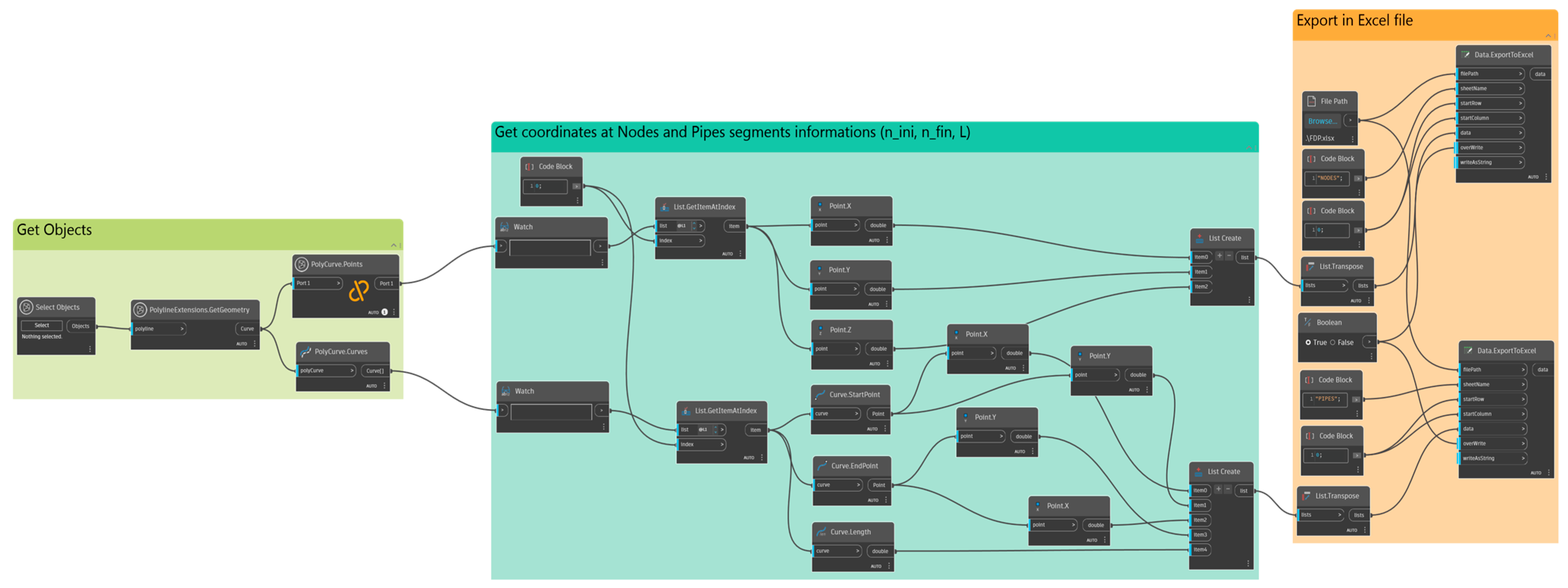
3.1. DyEHS Framework and Software Integration

The DyEHS toolchain is implemented within the environment of Autodesk AutoCAD Civil 3D (C3D) using Dynamo for visual programming and EPANET 2.2 for hydraulic analysis. Figure 1 illustrates the procedural flowchart of DyEHS (from data input to optimized design). The process begins with the user creating a preliminary layout of the water network in the C3D model. In our case study, this involves drawing 3D polylines or alignments representing the pipe paths on the site topography. Each node (junction or reservoir) and pipe in the network is thereby defined in a spatially accurate manner in the CAD/BIM model.

Using Dynamo, we developed custom scripts to extract the necessary data from the drawn network. In particular, a Dynamo script (referenced as polyinfo.dyn, shown in Figure 2) reads the geometric model and generates two text files: nodes.txt and pipes.txt. The nodes file contains information such as the node ID, coordinates, and elevation, while the pipes file contains the pipe ID, start node, end node, length, and any initial diameter assignment. These text files essentially translate the C3D drawing into a format suitable for hydraulic analysis. Once these files are created, a custom LISP (AutoLISP) routine called WRITE_INP (developed within the Visual Basic environment) is executed to convert the node and pipe data into an EPANET input file (*.inp). The resulting EPANET input file describes the network topology and demands. Using a built-in integration, this .inp file is then automatically opened in EPANET 2.2 from within the Civil 3D interface (Figure 3 depicts the EPANET model of the network loaded inside C3D). At this stage, the user has a baseline hydraulic model of the network within the BIM environment.

To show the capability of the tool in water distribution network design optimization, a real case study is shown. This case study is based on an Italian municipality called Bagnoli Irpino, situated in the south of Italy, and is based on the design of a new two-loops network that must provide a flow rate of approximately 10 L/s.

Figure 4 depicts an aerial image of the WDN under consideration with the position of a reservoir (yellow polygon) with a head equal to 735 masl. Once the 3D polyline has been drawn, by means of a Dynamo script, it is possible to retrieve two files: nodes.txt and pipes.txt.

The next step is to run the Harmony Search optimization for pipe sizing. DyEHS streamlines this by launching the HS optimizer directly from Civil 3D (Figure 5 shows the interface where the optimization is initiated inside C3D). Before running the optimizer, the user must prepare three input files for the optimization routine:

• *.inp file: the EPANET network input file (generated as described above), containing all nodes, pipes, demands, and initial pipe diameters (which can be nominal or all set to a maximum available size to start);
• *.dat file: a pipe cost data file that lists the available pipe diameters and their unit costs. This file begins with the number of available diameter options and the unit (e.g., millimeter), followed by each diameter and its cost per unit length;
• *.para file: a parameter file for the Harmony Search algorithm, specifying the values of the HS parameters and certain problem-specific settings.

For the Harmony Search to perform effectively, appropriate algorithm parameter values need to be provided. In this study, we set the HS parameters based on common recommendations from the literature:

• HMS (Harmony Memory Size): We used a memory size of 30 solution vectors (this is a typical value; smaller networks <10 nodes could use HMS = 20, and very large networks >100 nodes might use HMS = 50);
• HMCR (Harmony Memory Considering Rate): This is set to 0.95, meaning that there is a 95% chance that each decision variable in a new harmony is chosen from historically good values in the Harmony Memory rather than at random. A slightly lower HMCR like 0.90 is sometimes used for very small problems, and slightly higher one, up to 0.99, for very large problems;
• PAR (Pitch Adjustment Rate): This is set to 0.05, indicating a 5% chance of fine-tuning a chosen value (this is a standard default for HS);
• Flag_Skip and ECR: These are two parameters related to ensemble consideration in some HS variants; we set Flag_Skip to 1.0 and ECR to 0.0 as commonly recommended (effectively not using ensemble consideration);
• App_Cost: An approximate cost of an initial or typical design. In our case, this was estimated from a “normal” design (e.g., using a uniform pipe diameter that meets the minimum pressure) to scale the optimization (though this value is not critical for the HS algorithm, it can be used as a reference);
• MaxIter: The maximum number of iterations (HS improvisations) to perform. We chose a value (for example, 5000 hydraulic evaluations) that was high enough to allow for the convergence of the solution for the case study;
• MinHead: The minimum allowable head (pressure) at each node, which is a constraint in the design. For the case study, this was 25 m (meaning that each node must have at least 25 m of head, equivalent to roughly 2.5 bar pressure in the system).

Once these files are ready, the optimization can be executed. DyEHS passes the .inp, .dat, and .para files to the optimization engine (which runs an HS algorithm coded in a compatible language, e.g., Python or C#, accessible via Dynamo or a command line call). The EPANET toolkit is utilized by the optimizer to compute the network hydraulic state (node pressures and pipe flows) for each trial design. During the HS run, EPANET ensures that any proposed solution’s hydraulic constraints (continuity at nodes, energy equations in pipes, or pump curves, etc.) are satisfied, or that violations are detected (e.g., insufficient pressure).

Throughout the optimization process, the algorithm evaluates many candidate designs, but this is entirely automated and occurs in the background. The user simply waits for the algorithm to finish. Upon completion, DyEHS takes the best solution found (i.e., the set of pipe diameters that yields the minimum cost while meeting the pressure constraint of 25 m) and updates the Civil 3D model with these diameters. The result is an optimized BIM model of the WDN, where each pipe object in C3D now has the chosen diameter and all associated attributes. Additional Dynamo scripts and C3D routines then generate the detailed documentation and visualization of the design (plan views, profile drawings with hydraulic grade lines, and bill of materials, etc.). Figure 6 shows a portion of the final BIM model for the case study, including the pipe trenches, fittings, and appurtenances placed automatically by the software.

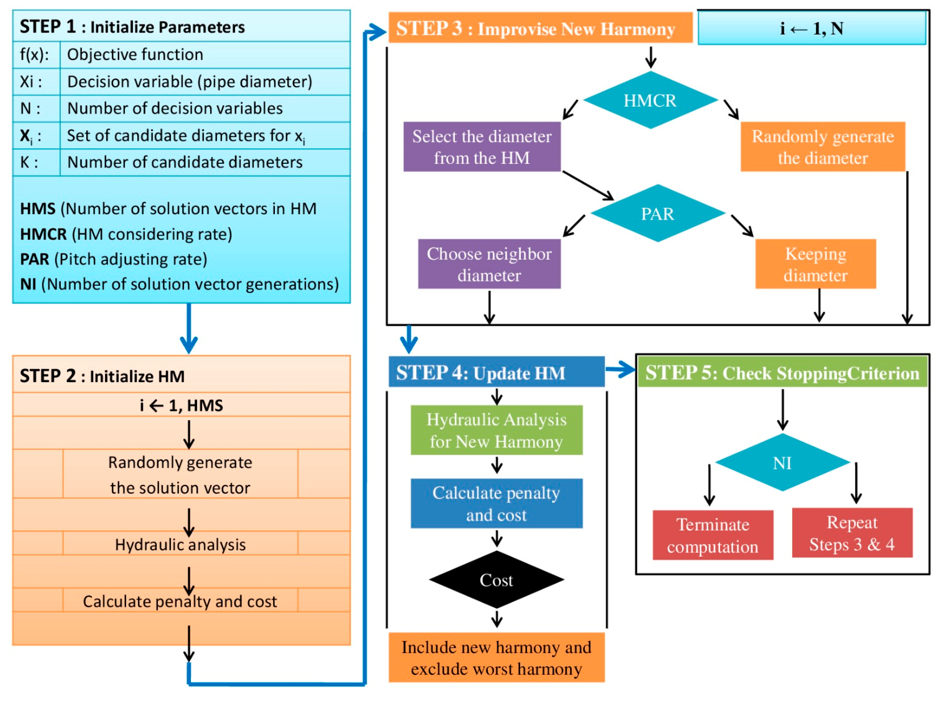
3.2. Harmony Search Optimization Procedure for WDN Design

The Harmony Search (HS) algorithm is central to the optimization step of DyEHS. In HS, each potential solution to the design problem is analogous to a musical harmony, and the process of finding a better design is akin to musicians improvising to find a pleasing harmony. We tailored the HS algorithm to the WDN pipe sizing problem as follows (Figure 7 presents a flow chart of the HS procedure as applied):

• Define Decision Variables: In WDN design, the decision variables are the diameters of the pipes. We considered a discrete set of commercially available pipe diameters (e.g., 50 mm, 75 mm, 100 mm, … up to 300 mm, etc.). Each pipe in the network can take one of these standard diameters. If there are N pipes, then a candidate design can be represented by an N-dimensional vector, where each element is an index corresponding to one of the available diameters. In our case study, for example, we had a set of diameter options for all pipes (ranging from 90 mm to 200 mm in ductile iron, as per the local standards) and the network comprised a certain number of pipes (decision variables equal to that number);
• Formulate the Objective Function: The objective is to minimize the total cost of the network. The cost has two main components: the capital cost of pipes and the operational cost (primarily pumping energy, if pumps are present). In our formulation for a gravity-fed network, the operational costs are minimal or zero, so the objective function simplifies to the sum of the pipe costs. Each pipe’s cost is the unit cost (from the .dat file) times its length. If pumps or energy were involved, we would include the annualized energy costs as well. Mathematically, we define the following:

  $$Minimize C={\sum }_{i=1}^N\left(c_{i}x{L}_i\right)+{\sum }_{j=1}^M{Energy}_j$$

  (1)

  where C is the total cost, ci is the unit cost of the i-th pipe based on its diameter, L_i is the length of the i-th pipe, and Energy_j is the pumping cost at the j-th pump (N total number of pipes and M total number of pumps);
• Impose Hydraulic Constraints: Any candidate design must meet the hydraulic feasibility. The primary constraint is that the pressure at all demand nodes must be ≥25 m (as specified by the design requirements). Other constraints include continuity of flow at nodes (the flow into each junction equals the flow out plus demand) and the headloss relationships (Hazen–Williams or Darcy–Weisbach equations) along pipes. When evaluating a design, EPANET is used to compute the node pressures and verify these constraints. Designs that violate the minimum pressure (25 m) at any node are considered unfeasible. In the HS algorithm, we handle this by penalizing such solutions heavily in the objective function (or by discarding them outright). In practice, during optimization, most randomly generated initial solutions will use large diameters to satisfy pressures, and then the algorithm tries to reduce the diameters to cut cost. The continuity and headloss constraints are inherently handled by EPANET’s hydraulic solver for each simulation;
• Initialize Harmony Memory: We randomly generate a set of HMS solutions (harmonies) that satisfy the constraints. To ensure feasibility, we may initially generate solutions biased towards larger diameters (so the pressures are likely met) and then use EPANET to check. Any unfeasible solution (with pressure < 25 m) is discarded and regenerated. The Harmony Memory is a matrix containing, say, 30 solution vectors, each with an associated cost. We then identify the best (lowest cost) and worst solutions in this memory;
• Improvise a New Harmony: This is the core of HS iteration. To create a new solution, for each pipe i (each decision variable), we decide whether to take a value from the Harmony Memory or to choose a new random value. This decision is governed by the Harmony Memory Considering Rate (HMCR). With probability (HMCR 0.95 in our case), we pick the pipe diameter from one of the existing solutions in the memory (i.e., we exploit known good designs). With probability (1–HMCR = 0.05), we choose a random diameter from the allowed set (exploration). If we chose from memory, we may then adjust it (with probability PAR = 0.05) to a neighboring diameter size (this mimics musical pitch adjustment, adding slight variation). For example, if the chosen memory value for a pipe is diameter 150 mm, a pitch adjustment might try 125 mm or 175 mm (the next lower or higher size in the list) with some small probability. This process is repeated for all pipes, resulting in a completely new design vector. We then run EPANET to evaluate the new design’s pressures and compute its cost;
• Update Harmony Memory: If the new harmony (design) is feasible and has a lower total cost than the worst solution in the current memory, it replaces the worst solution in the Harmony Memory. This ensures that the population of remembered solutions continuously improves or at least does not degrade. If the new solution is worse than the worst in memory, we may discard it (or in some implementations, there is a small chance to accept worse solutions to maintain diversity);
• Check for Convergence: Steps 5–6 are repeated iteratively. The process can terminate when a preset number of iterations (improvisations) is reached, or when the improvement in cost becomes negligible over several iterations (i.e., the algorithm has converged to a stable solution). In our implementation, we used a fixed number of iterations (MaxIter in the parameter file) as the stopping criterion. By that point, typically the improvements had leveled off.

Because EPANET is invoked at each solution evaluation, it automatically enforces the network flow continuity and computes pressures. Any candidate that does not meet the 25 m minimum pressure constraint is either penalized or filtered out. The HS algorithm thereby searches only within (or towards) the feasible region defined by EPANET’s hydraulic calculations. This coupling of HS with EPANET ensures that every design in the Harmony Memory is a hydraulically balanced network. The final outcome of HS optimization is the best harmony in memory, which corresponds to the lowest-cost design meeting all constraints.

For the case study network, Harmony Search proved effective in finding a cost-optimal combination of pipe diameters. Notably, because HS is a stochastic algorithm, multiple runs can yield slightly different solutions if there are near-equivalent designs. We ran the optimization several times to ensure the consistency of the results. In all runs, HS found the same minimum-cost layout (within a very small tolerance), giving confidence that the solution is at or very near the true global optimum for this network.

4. Results and Discussion

To demonstrate the capabilities of DyEHS, we applied it to a real-world case study of a municipal water distribution system. The case study is a proposed network in Bagnoli Irpino, a municipality in southern Italy, where a new distribution loop is being designed to improve the local water supply. The target network is a two-loop system that must deliver a peak flow rate of approximately 10 L/s to the service area. The water source is a reservoir located at an elevation (head) of 735 m above sea level, which provides gravity flow to the network.

Figure 4 shows an aerial view of the area, with the preliminary layout of the WDN superimposed. The network consists of one reservoir (water source), around 15 junction nodes (demand points at various elevations), and roughly 20 pipe segments forming two interlinked loops. The topography of the service area is moderately hilly, resulting in elevation differences that impact the pressure distribution. The design criterion is that even the highest node (in terms of elevation) should maintain at least 25 m of pressure head under the peak flow conditions. This requirement (MinHead = 25 m) was built into the optimization as discussed.

We chose a set of commercially available ductile iron pipes with diameters from 90 mm up to 200 mm for the design (with associated costs obtained from local supplier data, included in the .dat file). The cost per meter rises significantly with the diameter, motivating the optimizer to use smaller diameters wherever possible; however, using too small a diameter on a given link will increase the head loss and might violate the pressure constraint. Thus, the optimizer must find the right balance of pipe size to ensure that all nodes have ≥25 m head and the total cost is minimized.

Using DyEHS, the design process was as follows: We drew the network alignment in Civil 3D on the georeferenced map of Bagnoli Irpino (as shown in Figure 4). Each pipe segment’s length and each node’s elevation were thus accurately captured. Next, we ran the Dynamo scripts to export the network data and create the EPANET input file. We specified the demands at each node (based on the projected water use in that zone of the town) in the EPANET model. The initial diameters for all pipes were set to a relatively large size (200 mm) in the EPANET file to ensure that the initial hydraulic simulation had no pressure shortfalls. At this point, an initial hydraulic analysis showed that with all 200 mm pipes, the minimum pressures were well above 25 m—meaning that the system could likely use smaller pipes and still meet the requirements.

We then prepared the HS parameter file. The approximate cost of a “normal” design (App_Cost) was estimated by sizing pipes using a traditional method (gradually reducing the diameters from the source outward until pressures hit ~25 m). This gave a ballpark figure to guide the optimization, though the algorithm does not strictly require it. The HS parameters were set as described earlier (HMS = 30, HMCR = 0.95, etc.). The optimizer was launched from within Civil 3D (Figure 2). Over about 3000 iterations, the HS algorithm iteratively improved the network design. The convergence was observed in terms of cost: it started with a very high cost (all pipes 200 mm) and quickly dropped as the algorithm tried smaller sizes. By iteration ~500, a near-optimal solution was found, and minor adjustments continued to iteration 3000 with negligible further improvement.

The optimized design selected by DyEHS had a mix of pipe diameters: the pipes nearest the reservoir and on the primary loop were relatively larger (150–175 mm) to carry the higher flows with minimal head loss, whereas the pipes on the downstream loops and branches were smaller (90–125 mm), since the flows there were lower and the pressure could be maintained with smaller sizes. All junction pressures in the EPANET analysis of the final design were at or above 25 m, satisfying the constraint. The total cost of the optimized network was substantially lower than an initial uniform diameter design—DyEHS achieved about a 15% cost reduction compared to a design where all the pipes were, say, 150 mm (a common heuristic design choice). This cost saving is significant for infrastructure projects, illustrating the benefit of optimization.

Crucially, DyEHS not only provided the numbers (diameters), but also automatically updated the BIM model in Civil 3D. Figure 6 depicts a segment of the network in the finalized C3D model. In the figure, one can see the trenches for pipeline installation and placed appurtenances (e.g., valves at certain junctions). The model is fully annotated with pipe diameters and can be used to extract profiles (long sections) of each pipe run. These profiles show the ground elevation, the pipe invert elevation, and the hydraulic grade line (HGL) along the pipe—confirming that the HGL stays above the minimum required (which corresponds to the 25 m head at the critical node). The BIM model also serves for generating plan drawings and computing material quantities (total length of each diameter of pipe, number of bends, and valves, etc., which were identified through Dynamo scripts). All of this information is available immediately after optimization, which demonstrates a significant improvement in the workflow efficiency.

By integrating the optimization into the BIM environment, any changes to the layout (for instance, if the alignment of a pipe had to be adjusted due to a site constraint) can be accommodated and the optimization re-run quickly to update the design. This tight coupling of design and analysis ensures that the final plans are consistent with the optimized solution, reducing the chances of error that might occur if the data were transferred manually between separate software.

In summary, the case study application showed that DyEHS could successfully produce an optimal design for a real WDN with minimal user effort beyond providing the initial layout and parameters. The next section presents the results in more detail and discusses the performance and implications of using DyEHS for WDN design.

Therefore, from txt files with the aim of a LISP tool, implemented in the Visual Basic environment, it is possible to obtain an .inp file (WRITE_INP) and open the file pipe.inp directly from the C3D environment in EPANET 2.2 (Figure 3).

The application of the DyEHS tool to the Bagnoli Irpino network yielded an optimized design that meets the system’s requirements at a minimized cost. In this section, we discuss the results of the optimization and the broader implications, including the computational performance, comparison to traditional design, and the benefits of BIM integration.

The Harmony Search algorithm converged on a solution where the pipe diameters varied strategically throughout the network. The highest pressure headloss occurred in pipes carrying the largest flow (near the reservoir), so those pipes were assigned larger diameters to keep the headloss low. Further from the source, smaller diameters sufficed. The final design had no node, with the pressure below 25 m under peak demand. EPANET’s hydraulic output for the optimized design showed that the minimum pressure was about 26.8 m at the critical node (the node at the highest elevation and farthest hydraulic distance), indicating that the constraint was active but satisfied. Most other nodes had a higher pressure (30–50 m), which is acceptable within the design range. The total cost of the pipes in this solution was approximately 85% of the cost of a uniform-diameter design meeting the same pressure criteria, reflecting a considerable saving in materials. This aligns with typical outcomes in the WDN optimization literature, where savings of 10–20% are often reported when using algorithms versus manual or uniform sizing.

It is worth noting that the optimization process inherently found a balance between capital cost and hydraulic performance. If we forced even smaller diameters, some node pressures would drop below 25 m, incurring a penalty and thus a higher effective cost in the optimization’s objective function. The HS algorithm, by exploring various combinations, effectively located the point where any further cost reduction (using smaller pipes) would violate the constraints and thus not truly be feasible. In the absence of pumps, all operational cost considerations boiled down to maintaining adequate gravity pressure, which the algorithm handled via the pressure constraint.

The runtime for the HS optimization in this network was on the order of a few minutes on a standard engineering workstation. Each EPANET hydraulic simulation is very fast (fractions of a second for a network of this size), so the majority of time was spent in the iterative loop of the metaheuristic algorithm. Using HMS = 30 and MaxIter = 3000, a total of 90,000 network evaluations were performed. This may sound high, but because EPANET solves the network hydraulics efficiently, the overall time remained reasonable. We observed that the solution quality plateaued well before the maximum iterations—by around 2000 iterations the algorithm was essentially oscillating around the optimum. This suggests that we could potentially use a convergence-based stopping criterion to reduce the runtime. If needed, parallel computing could also be employed (since many hydraulics evaluations are independent) or a smaller Harmony Memory could be tested. However, given the few minutes runtime, the current setup is acceptable for practical use in networks of similar scale. For much larger networks (hundreds of pipes), computational efficiency would be a concern, and one might consider more advanced techniques like parallel HS or hybrid methods. Recent studies have employed parallelization (e.g., GPU-based hydraulic calculations or improved heuristics) to handle large-scale WDN optimizations, which could be integrated into future versions of DyEHS.

Traditionally, an engineer might design this network by selecting the pipe diameters based on experience or simplified calculations (e.g., using the Hazen–Williams equation and trial adjustments). Such a manual approach might ensure that the minimum pressure is met, but it often results in over-designed (oversized) pipes to provide a safety margin. DyEHS, on the other hand, finds the minimum sufficient sizes for each pipe, effectively removing excess conservatism while still respecting the constraints exactly. This leads to lower costs. In our case, a manual design might have used, for example, mostly 150 mm pipes throughout to be safe, whereas DyEHS pinpointed that some segments could be 125 mm or 100 mm without issue. Furthermore, the automated approach eliminates human error in calculating head losses and frees up the engineer’s time. It is important, however, for the engineer to review the optimized solution—occasionally, algorithms might exploit a constraint in a way that is technically acceptable but operationally undesirable (for instance, using very small pipes that meet the minimum pressure but result in high velocity, which could be a concern for transients or water quality). In this study’s results, all velocities were within the typical design limits (generally below 2 m/s in peak flow), and the solution appeared to be well balanced and practical.

One of the most significant advantages observed was the seamless creation of a detailed BIM model of the optimized network. In conventional workflows, once optimization has been carried out (perhaps in a separate tool or script), one has to manually implement those results into a CAD drawing—a process prone to errors and omissions. Here, because the optimization was embedded in Civil 3D, the final diameters were automatically applied to the drawing elements. As shown in Figure 3, the 3D model of the network includes every pipe with its specific diameter, as well as the automatically placed standard fittings (bends, tees, and junctions), because the software can detect network connectivity and insert appropriate components from its parts library. This level of detail is extremely useful for downstream activities: generating excavation profiles, estimating excavation volumes, and even visualizing the network in relation to other underground utilities. The model also facilitated creating plan and profile drawings that are often required for construction documentation. These drawings were generated by Civil 3D with minimal additional drafting, since the pipe alignments and profiles were already defined—an example profile sheet was produced showing the ground level, pipe invert, and hydraulic grade, which helped in verifying that the pressure constraint was satisfied along the pipeline’s extent.

The integrated approach also supports iterative design refinement. For example, if a certain pipe was found to be too shallow or too deep when checking clash detection with other utilities, the alignment could be adjusted in Civil 3D and the optimization re-run to adapt the diameters to the new scenario. This tight feedback loop can greatly reduce the time between conceptual design and the final construction drawings. It exemplifies the concept of a “digital twin” for design—the digital model is not just a static representation, but also an active participant in the optimization and decision-making process.

Harmony Search proved to be a suitable algorithm for this problem, yielding good results without excessive tuning. The choice of the HS parameters was based on guidelines and did not require a calibration run in this case; however, the performance of any metaheuristic algorithm can depend on the parameter settings. Reviewer feedback pointed out the importance of parameter optimization. In response, we note that our HS parameters (HMS, HMCR, and PAR, etc.) were set to standard values that generally work well. We did experiment with a slightly smaller Harmony Memory and higher HMCR; the differences in results were minor, indicating that HS is fairly robust for this application. In future work, one could implement an adaptive HS where parameters like PAR or HMCR evolve during the run, potentially speeding up the convergence. Additionally, combining HS with another method (for example, using a GA to seed the initial Harmony Memory) could be explored for even better performance. Nonetheless, given the network size and complexity, HS alone performed adequately, finding the optimum design reliably across multiple runs.

Although our optimization focused on a single demand scenario (peak demand) and a single objective (cost), the results have implications for system resilience and long-term operation. By minimizing the cost while satisfying the minimum pressure, the design inherently does not have a lot of excess capacity. This is economical, but it also means that there is limited buffer for unexpected demand increases or pipe outages. In practice, engineers might prefer a design with some extra safety margin. This could be incorporated by slightly tightening the pressure constraint (e.g., require 30 m minimum instead of 25 m in the optimization), or by explicitly adding a resilience objective as discussed earlier. Our study demonstrates the baseline optimal solution; decision-makers can then decide if they want to invest more for additional resilience. It is encouraging to see that modern optimization studies address reliability by including metrics like the resilience index. For this case, the network is small and fed from one source, so reliability improvements might require redundancy (like a second feed or a loop closure), which was outside the scope of our design.

Another point of discussion is the environmental impact and long-term maintenance costs of the network, which were not explicitly included in our optimization model. While we minimized the initial construction cost, a truly sustainable design might consider the life-cycle cost—including energy consumption (if pumps are used), pipe breakage rates, and replacement costs over the system’s life. In our gravity system case study, energy is not a factor, but if this were an urban system with pumping, one could incorporate the pumping energy (with associated carbon emissions) into the objective. Recent research advocates for life-cycle cost analysis and optimization for WDNs, which includes the carbon footprint of materials and energy. Additionally, pipe diameter choices have maintenance implications: larger diameters might last longer before needing replacement and can handle future demand growth, whereas smaller diameters are cheaper now but could incur earlier upgrades if demand grows. Some studies have formulated multi-objective models to minimize cost, maximize the remaining service life, or minimize the break risk, etc. For simplicity, our current study did not model these factors, but in the discussion, we acknowledged that environmental and maintenance costs should be considered in a comprehensive design. For example, using slightly larger pipes might reduce water velocities, potentially lowering pipe friction deterioration and leak probabilities over time—an indirect maintenance benefit. A life-cycle optimization approach could assign a cost to future pipe rehabilitation, so that the algorithm might choose a design that is not the absolute cheapest upfront, but has a lower total cost over (say) 30 years. In future applications of DyEHS, especially to larger networks, we plan to extend the objective function to incorporate such long-term factors, possibly using a multi-objective HS or a weighted sum approach to trade off initial cost vs. future costs.

In summary, the results demonstrate the effectiveness of DyEHS for optimal WDN design and highlight several discussion points: the efficiency of metaheuristic optimization (like HS) in finding cost-effective designs, the integration of BIM, which greatly aids in moving from computation to implementation, and the need to consider broader factors such as reliability, environmental impact, and maintenance in design optimization. The case study shows a tangible benefit (cost saving and automated model generation), which would likely be even more pronounced in larger or more complex projects.

5. Limitations of the Study

While this research introduces a powerful integrated tool and demonstrates its benefits, there are certain limitations to acknowledge:

• The current implementation of DyEHS optimizes only the initial construction cost (with a pressure constraint). It does not explicitly account for other objectives such as system resilience, water quality, or life-cycle cost. As a result, the optimized design is cost-effective, but may have limited redundancy or adaptability. In practice, engineers might prefer a slightly more robust design than the absolute minimum-cost solution. Future extensions could incorporate multi-objective optimization to address these aspects;
• Related to the above, environmental and long-term maintenance costs were not included in the optimization model. Factors like energy consumption (for pumped systems), pipe corrosion rates, leakage, and eventual replacement costs are important for sustainability. Our study optimized for present cost only, which could lead to higher expenses over the network’s lifespan. Integrating a life-cycle cost assessment (LCC) would allow DyEHS to suggest designs that are optimal in the long run, not just at installation;
• The DyEHS framework is built around Autodesk Civil 3D, Dynamo, and EPANET. This means the toolchain currently works only for users who have access to these software. This could limit accessibility for some practitioners. Additionally, there may be a learning curve associated with using Dynamo and custom scripts. While BIM integration is advantageous, it ties the solution to a particular platform. In the future, developing a more platform-agnostic or open-source version (e.g., using FreeCAD/Revit with open EPANET libraries) would broaden usability;
• Although we used standard HS parameters and the algorithm performed well, metaheuristic algorithms do carry some sensitivity to parameter choices and random seed. There is no guarantee that the chosen HS parameters are optimal for every network. If applied to a very different case (e.g., a much larger network or one with pumps and tanks), HS might require retuning, or even a different algorithm. Moreover, as with any heuristic algorithm, there is a small chance that it could converge to a local minimum, especially if the search space is extremely complex. We mitigated this via multiple runs and found consistent results, but this might not hold universally;
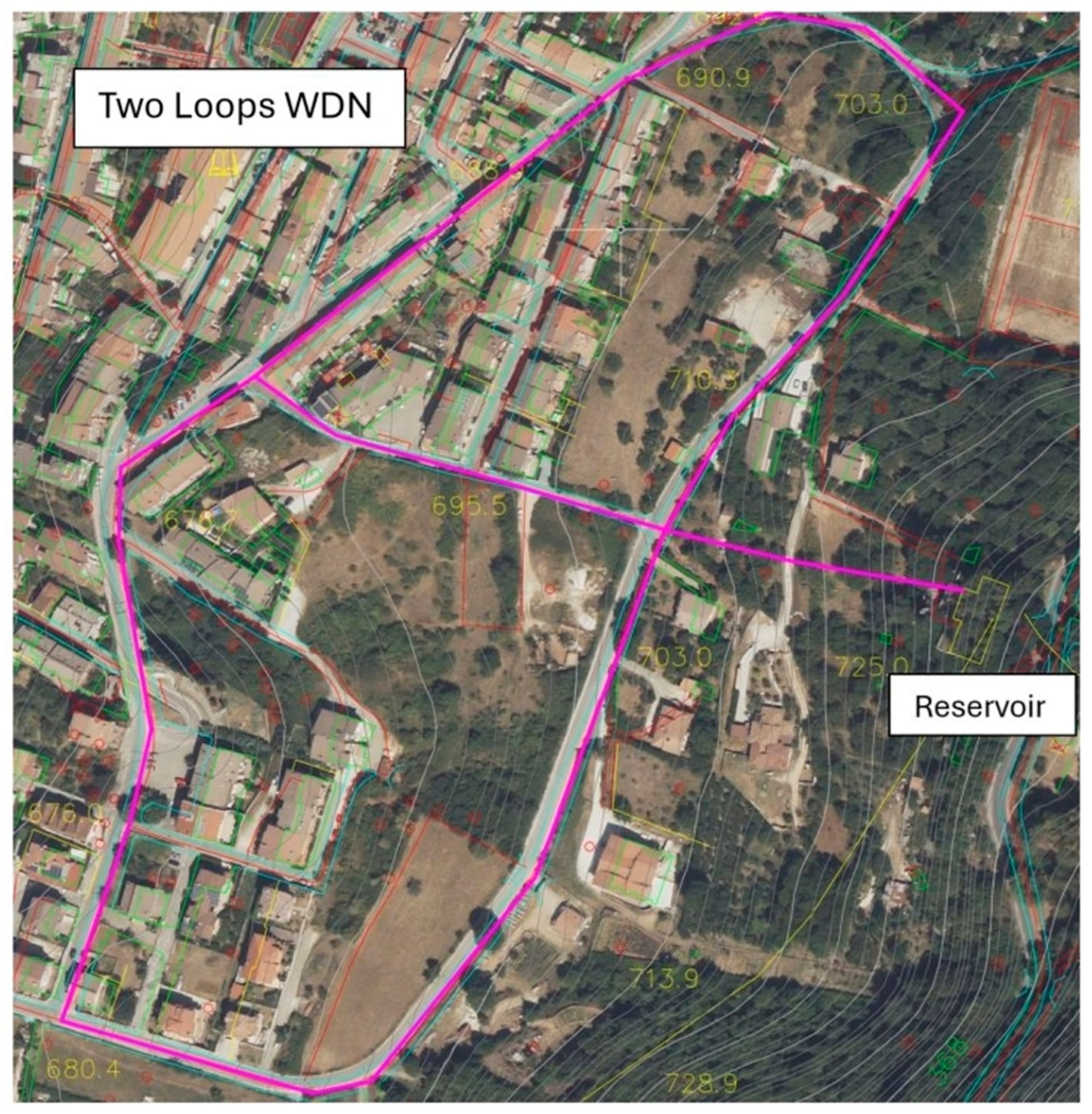
• The demonstration was on a medium-sized network (two-loop system). The performance of DyEHS on very large networks (hundreds of pipes or multiple sources) remains to be tested. Computational time could become a limiting factor in larger problems, and integration within a BIM environment might face challenges with very large datasets (e.g., Civil 3D handling hundreds of pipe objects dynamically). The methodology is sound for larger cases, but practical runtime and software memory limits could pose challenges;
• DyEHS automates much of the design, but the quality of the outcome still depends on the user providing reasonable inputs—such as accurate demand estimates, appropriate constraints, and realistic cost data. Garbage-in, garbage-out applies; if any input is off (say, costs are not accurate or a demand is grossly underestimated), the optimized design could be misleading. Thus, a knowledgeable engineer must supervise the process, interpret the results, and possibly override the pure optimization outcome if it conflicts with practical considerations (e.g., standard practice or safety factors);
• The workflow was tailored to gravity-fed distribution networks. If one introduces pumps, valves, or complex controls, the optimization problem becomes more complicated (optimizing pump operations or control settings in tandem with pipe sizing). DyEHS in its current form handles pipe sizing. Additional decision variables like pump scheduling or valve placement would require expanding the optimization algorithm and integration (the references show initial work by the authors on using HS for valve placement, which could be integrated in the future). So, the present study is limited to the pipe sizing aspect of WDN design.

Despite these limitations, the study provides a foundation for a more comprehensive tool. Acknowledging these constraints allows us to improve DyEHS further. For instance, adding a module for life-cycle analysis would address the long-term cost issue; testing on larger networks would help to gauge scalability; and possibly incorporating other algorithms or parallel computing could ensure performance across diverse scenarios.

6. Conclusions

This study presented DyEHS, an integrated BIM-based tool that combines Civil 3D, Dynamo, EPANET, and the Harmony Search algorithm for the optimal design of water distribution networks. DyEHS allows engineers to automate the pipe sizing process within a familiar design environment, significantly improving the workflow efficiency.

In a real-world application to the Bagnoli Irpino WDN, DyEHS reduced the total pipe costs by approximately 15% compared to a uniform diameter design, while ensuring hydraulic feasibility (minimum node pressure ≥ 25 m). The optimized design was automatically reflected in a detailed 3D BIM model, ready for documentation and construction planning.

The integration of optimization into the BIM workflow proved particularly valuable, enabling rapid iterations, automatic updates, and consistent hydraulic validation. By eliminating the need for manual data transfer between design and analysis tools, DyEHS offers a practical and efficient solution for modern infrastructure projects.

While the tool focuses on minimizing capital costs, it does not yet account for multi-objective considerations such as system resilience, energy consumption, or life-cycle costs. Expanding DyEHS to incorporate these dimensions will enhance its applicability to more complex and sustainability-driven projects. Future developments will focus on the following:

• Integrating multi-objective optimization (cost, resilience, and environmental impact);
• Enhancing algorithmic performance via parallel processing or hybrid metaheuristics;
• Developing a platform-agnostic version to increase accessibility beyond Autodesk users;
• Extending DyEHS to handle pumped systems, storage tanks, and dynamic demand scenarios for broader application.

References

1. Zhao, L.; Liu, Z.; Mbachu, J. An Integrated BIM–GIS Method for Planning of Water Distribution System. ISPRS Int. J. Geo-Inf. 2019, 8, 331. [Google Scholar] [CrossRef]
2. Ramani, K.; Rudraswamy, G.K.; Umamahesh, N.V. Optimal Design of Intermittent Water Distribution Network Considering Network Resilience and Equity in Water Supply. Water 2023, 15, 3265. [Google Scholar] [CrossRef]
3. Wu, Y.; Ma, W.; Miao, Q.; Wang, S. Multimodal continuous ant colony optimization for multisensor remote sensing image registration with local search. Swarm Evol. Comput. 2019, 47, 89–95. [Google Scholar] [CrossRef]
4. Morley, M.; Tricarico, C. Hybrid Evolutionary Optimization/Heuristic Technique for Water System Expansion and Operation. J. Water Resour. Plan. Manag. 2015, 142, C4015006. [Google Scholar] [CrossRef]
5. Vertommen, I.; van Laarhoven, K.; Cunha, M.D.C. Robust Design of a Real-Life Water Distribution Network under Different Demand Scenarios. Water 2021, 13, 753. [Google Scholar] [CrossRef]
6. Alperovits, E.; Shamir, U. Design of optimal water distribution systems. Water Resour. Res. 1977, 13, 885–900. [Google Scholar] [CrossRef]
7. Quindry, G.E.; Brill, E.D.; Liebman, J.C. Optimization of Looped Water Distribution Systems. J. Environ. Eng. Div. 1981, 107, 665–679. [Google Scholar] [CrossRef]
8. Simpson, A.R.; Dandy, G.C.; Murphy, L.J. Genetic Algorithms Compared to Other Techniques for Pipe Optimization. J. Water Resour. Plan. Manage. 1994, 120, 423–443. [Google Scholar] [CrossRef]
9. Gessler, J. Pipe network optimization by enumeration. In Computer Applications in Water Resources; ASCE: Fort Collins, CO, USA, 1985; pp. 572–581. [Google Scholar]
10. Loubser, B.F.; Gessler, J. Computer-aided optimization of water distribution networks. Civ. Engr. S. Afr. 1990, 32, 413–422. [Google Scholar]
11. Loganathan, G.V.; Greene, J.J.; Ahn, T.J. Design Heuristic for Globally Minimum Cost Water-Distribution Systems. J. Water Resour. Plan. Manage. 1995, 121, 182–192. [Google Scholar] [CrossRef]
12. da Conceicao Cunha, M.; Ribeiro, L. Tabu search algorithms for water network optimization. Eur. J. Oper. Res. 2004, 157, 746–758. [Google Scholar] [CrossRef]
13. Murphy, L.J.; Simpson, A.R. Genetic algorithms In Pipe Network Optimization; Research Report R93; University of Adelaide: Adelaide, Australia, 1993. [Google Scholar]
14. Dandy, G.C.; Simpson, A.R.; Murphy, L.J. An Improved Genetic Algorithm for Pipe Network Optimization. Water Resour. Res. 1996, 32, 449–458. [Google Scholar] [CrossRef]
15. Savic, D.A.; Walters, G.A. Genetic Algorithms for Least-Cost Design of Water Distribution Networks. J. Water Resour. Plan. Manage. 1997, 123, 67–77. [Google Scholar] [CrossRef]
16. Storn, R.; Price, K. Differential evolution—A simple and efficient heuristic for global optimization over continuous spaces. J. Glob. Optim. 1997, 11, 341–359. [Google Scholar] [CrossRef]
17. Maier, H.R.; Simpson, A.R.; Zecchin, A.C.; Foong, W.K.; Phang, K.Y.; Seah, H.Y.; Tan, C.L. Ant Colony Optimization for Design of Water Distribution Systems. J. Water Resour. Plan. Manage. 2003, 129, 200–209. [Google Scholar] [CrossRef]
18. Geem, Z.W.; Kim, J.H.; Loganathan, G.V. A new heuristic optimization algorithm: Harmony Search. Simulation 2001, 76, 60–68. [Google Scholar] [CrossRef]
19. De Paola, F.; Galdiero, E.; Giugni, M. Location and Setting of Valves in Water Distribution Networks Using a Harmony Search Approach. J. Water Resour. Plan. Manage. 2017, 143, 04017015. [Google Scholar] [CrossRef]
20. Fujiwara, O.; Khang, D.B. A two-phase decomposition method for optimal design of looped water distribution networks. Water Resour. Res. 1990, 26, 539–549. [Google Scholar] [CrossRef]
21. Gupta, I.; Gupta, A.; Khanna, P. Genetic algorithm for optimization of water distribution systems. Environ. Model. Softw. 1999, 14, 437–446. [Google Scholar] [CrossRef]
22. Eusuff, M.M.; Lansey, K.E. Optimization of Water Distribution Network Design Using the Shuffled Frog Leaping Algorithm. J. Water Resour. Plan. Manage. 2003, 129, 210–225. [Google Scholar] [CrossRef]
23. Geem, Z.W. Optimal cost design of water distribution networks using harmony search. Eng. Optim. 2006, 38, 259–277. [Google Scholar] [CrossRef]
24. Sirsant, S.; Reddy, M.J. Improved MOSADE algorithm incorporating Sobol sequences for multi-objective design of Water Distribution Networks. Appl. Soft Comput. 2022, 120, 108682. [Google Scholar] [CrossRef]
25. Todini, E. Looped water distribution networks design using a resilience index based heuristic approach. Urban Water 2000, 2, 115–122. [Google Scholar] [CrossRef]
26. Alvisi, S.; Franchini, M. A heuristic procedure for the automatic creation of district metered areas in water distribution systems. Urban Water J. 2014, 11, 137–159. [Google Scholar] [CrossRef]
27. Ayala-Cabrera, D.; Piller, O.; Deurlein, J.; Herrera, P. Key performance indicators to enhance water distribution network resilience in three-stages. Water Util. J. 2018, 19, 79–90. [Google Scholar]
Figure 1. DyEHS flow chart procedure proposed.
Buildings 15 01694 g001
Figure 2. polyinfo.dyn script implemented in Dynamo environment.
Buildings 15 01694 g002
Figure 3. Digital model of water distribution network in EPANET 2.2 environment inside C3D.
Buildings 15 01694 g003
Figure 4. Two-loops WDN of Bagnoli Irpino, Campania Region (south of Italy).
Buildings 15 01694 g004
Figure 5. HS network optimizer launched from C3D environment.
Buildings 15 01694 g005
Figure 6. BIM model of a portion of networks implemented (with excavation trench, fittings, and appurtenances).
Buildings 15 01694 g006
Figure 7. HS optimizer flow chart (adapted from Geem, 2006 [17]).
Buildings 15 01694 g007