Abstract
In this study, experiments were conducted on the freeze–thaw performance of manufactured sand cement concrete with different sand ratios and fly ash contents. The research found that during 200 freeze–thaw cycles, as the fly ash content increased, the concrete exhibited a higher mass loss rate and a decline in the relative dynamic modulus of elasticity. This was due to the lower activity of SiO2 and Al2O3 in the fly ash, which reduced the hydration products. Incorporating an optimal amount of manufactured sand can increase the density of concrete, thereby improving its resistance to freeze–thaw cycles. However, when the content of manufactured sand was high, its large surface area could interfere with the hydration process and reduce strength, thereby diminishing the freeze–thaw resistance of the concrete. Given that studying the freeze–thaw resistance of manufactured sand concrete is time-consuming and influenced by many factors, a prediction model based on a BP (back propagation) neural network was developed to estimate the mass loss rate and the relative dynamic modulus of elasticity following freeze–thaw cycles. After validation, the model was found to be highly reliable and could serve as a foundation for mix design decisions and freeze–thaw performance prediction of manufactured sand cement concrete.
1. Introduction
In recent years, low-carbon sustainability has been a key focus of research in the construction industry [1]. Many scholars have explored this direction, such as using recycled aggregates to replace natural aggregates in the production of recycled concrete [2], using fly ash to partially replace cement as a binder in concrete [3], incorporating straw fibers into concrete for modification [4], and substituting natural river sand as fine aggregate in concrete with manufactured sand [5]. The focus of this study is on the preparation of concrete using manufactured sand to investigate its impact on frost resistance. Natural river sand is an irreplaceable resource [6]. However, the accelerated global urbanization process has led to the over-extraction of natural sand, causing significant environmental damage [7]. From an economic perspective, the production cost of manufactured sand is typically lower than that of natural river sand. This is because the raw materials for manufactured sand primarily come from construction waste, which ensures a more stable supply and relatively lower prices. In contrast, the price of river sand continues to rise due to its gradual depletion, making the use of manufactured sand an effective way to reduce material costs in construction [8]. Jadhav et al. found that replacing 60% of natural sand with manufactured sand not only achieved good strength but also reduced costs by approximately 10–15% in their study on the feasibility of using manufactured sand to replace natural river sand in concrete production [9]. From an environmental protection perspective, the excessive extraction of natural river sand often leads to riverbed subsidence, resulting in a series of ecological issues [10]. According to Gupta et al., using manufactured sand as a substitute for river sand in construction not only reduces pollution from waste accumulation but also decreases river sand extraction by approximately 30% to 50%, which is significant for protecting rivers and surrounding ecosystems [11]. More importantly, the localized production of manufactured sand can reduce carbon emissions by 20% to 30% compared to the long-distance transportation of river sand [12]. As a result, substituting natural sand with manufactured sand as fine aggregate in concrete has become a research focus [13].
Manufactured sand particles are angular and rough, with a coarse and porous texture [14]. Therefore, the angular shape and contour of manufactured sand can affect the compressive strength, flexural strength, and dynamic modulus of manufactured sand concrete [15]. Many scholars have already conducted various studies on manufactured sand concrete. Jin et al. [16] researched the fatigue life of manufactured sand concrete beams and found that their fatigue life is associated with the range of applied load or stress. Li et al. [17] studied the abrasion resistance of manufactured sand cement concrete and found that the roughness and angularity of manufactured sand significantly enhance its abrasion resistance compared to conventional concrete. The optimal performance was achieved upon reaching 10% stone powder content in the manufactured sand. Shen et al. [18] used sandstone-derived manufactured sand to prepare ultra-high-strength concrete. Their research found that the hydration products of manufactured sand were much finer than those in conventional concrete, resulting in higher strength compared to concrete made with river sand. Li et al. [19] studied the effects of manufactured sand on the properties of both low-strength and high-strength concrete. The results indicated that when the stone powder content in the manufactured sand ranged from 0% to 20%, the chloride ion permeability and frost resistance of low-strength concrete decreased to varying extents, whereas high-strength concrete was almost unaffected. Riyadh et al. [20] quantified the shape characteristics of manufactured sand, providing better control methods for the workability of manufactured sand cement concrete. Prakash et al. [21] used manufactured sand to prepare self-compacting concrete. Due to the larger surface area of the manufactured sand particles, a higher volume of paste is required during preparation. Experimental verification showed that, although theoretically more paste is needed, the substantial amount of fines in the manufactured sand effectively fills the required paste volume. Therefore, using manufactured sand to produce self-compacting concrete is feasible. Cai et al. [22] studied the fracture mechanics of manufactured sand cement concrete with the addition of steel fibers. The research found that adding steel fibers significantly improved its load-bearing capacity and post-peak behavior. As the volume fraction of steel fibers increased, the concrete’s post-peak behavior changed from quasi-brittle to ductile, and its residual strength also increased accordingly. Wang et al. [23] prepared high-strength concrete (HMC) with manufactured sand from different sources and studied its bonding performance with steel reinforcement. The tests revealed that as the content of stone powder in the manufactured sand increased, the bond strength between the HMC and the steel reinforcement initially increased and then decreased. Finally, by fitting the experimental data, they obtained a bond-slip constitutive model for HMC and steel reinforcement. Zhu et al. [24] determined the carbon emission factors for manufactured sand and manufactured sand gravel in their study and calculated the carbon emissions of manufactured sand concrete (MSC). They used the Gaussian distribution function to fit the variations in compressive strength and carbon reduction rate of MSC under different stone powder replacement rates and fly ash replacement rates. Wang et al. [25] tested the performance of manufactured sand cement concrete at high temperatures and analyzed the factors affecting its performance under such conditions. They used measured stress–strain curves and existing high-temperature behavior constitutive models to conduct their analysis. Yang et al. [26] tested the carbonation depth of reinforcement in MSC with different amounts of stone powder and used scanning electron microscopy (SEM) to analyze the carbonation mechanism of MSC. The test results showed that with the increase in stone powder content, the carbonation depth and corrosion probability of the reinforcement initially decreased and then increased. Zhao et al. [27] prepared concrete of different strength grades using both basic and optimized dosages of water-reducing agents. The test results indicated that the optimized dosage of water-reducing agents significantly improved the flowability, peak stress, and elastic modulus of artificial sand concrete at the same strength grade, while reducing slump loss, peak strain, and porosity.
Although there has been extensive research on the strength of manufactured sand cement concrete, studies on its freeze–thaw resistance are still relatively scarce. Piotr et al. [28] studied the freeze–thaw resistance of concrete prepared with waste foundry sand as a replacement for natural sand. Their experiments revealed that adding 5% waste foundry sand resulted in a mass loss of 6.31% after 180 freeze–thaw cycles, which is more than double that of ordinary concrete. However, when the waste foundry sand content was increased to 15%, the mass loss slightly decreased to 5.1%. Processing iron tailings into fine sand as a substitute for natural river sand holds considerable potential. Shi et al. [29] employed the entropy weight method to develop a Weibull damage model to assess the freeze–thaw cycle performance of concrete made with iron tailings sand. The findings revealed that damage in the concrete progresses from the edges of the specimen toward the center, with damage levels ranging between 28% and 44%.
With the advancement of modern computing technology, artificial neural networks (ANNs) have found widespread application in traditional engineering fields, offering reliable connections between inputs and outputs [30]. ANNs are a nonlinear data modeling approach inspired by the functioning of biological neural networks for processing information [31]. These networks generally consist of three types of layers: an input layer, an output layer, and one or more hidden layers. Information is transmitted and processed through neurons, which, after weighted modifications, generate a nonlinear output [32]. To date, neural network prediction models have seen extensive application in research on manufactured sand concrete [33,34,35,36,37]. Himank et al. [35] utilized artificial neural network technology to predict the mechanical properties of waste foundry sand concrete. Upon comparing the predicted results with experimental outcomes, they found that the reliability coefficients for compressive strength and tensile strength reached 0.9007 and 0.9022, respectively. This demonstrates the model’s high accuracy and practical value. Gottapu et al. [38] developed a neural network prediction model based on the Levenberg–Marquardt (LM) algorithm and the Steepest Descent (SD) algorithm to assess the mechanical properties of fiber-reinforced concrete made with various fiber percentages and manufactured sand as a replacement for natural sand. The results indicated that the LM algorithm required fewer iterations and produced more accurate predictions than the SD algorithm, with an accuracy of up to 95%.
Since manufactured sand replaces natural river sand in manufactured sand cement concrete, various properties will change significantly. However, current research on the frost resistance of manufactured sand concrete is limited, and using neural networks to predict its frost resistance indicators is even rarer. This paper investigates the mass loss rate and relative dynamic modulus of elasticity of manufactured sand cement concrete following freeze–thaw cycles. We also developed a BP neural network prediction model to assess its effectiveness in forecasting the frost resistance of manufactured sand concrete.
2. Materials and Methods
2.1. Raw Materials
2.1.1. Binder
The cement used in this experiment is Conch brand P·O 42.5 ordinary Portland cement (OPC), produced by Anhui Conch Cement Company, China (Wuhu, China). Refer to Table 1 for the performance test results. All the indicators in the table meet Chinese standard GB175-2023 [39].

Table 1.
Various indicators of cement.
2.1.2. Aggregates
The strength of cement concrete pavement comes from the cementing strength of the concrete mixture. Three different sizes of limestone aggregates used in the experiment were from Suzhou Sanchuang Pavement Engineering Co., Ltd., Changshu, China, as shown in Figure 1. The performance test results of the aggregates are shown in Table 2. The aggregates used in the experiment meet the relevant requirements of Chinese standard JTG 3432-2024 [40].
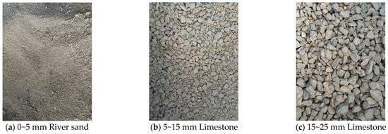
Figure 1.
Aggregates of different particle sizes.
Table 2.
Aggregate performance.
2.1.3. Fly Ash
The fly ash utilized in this research is Grade II fly ash produced by Henan Jiewei Environmental Materials Company, Zhengzhou, China. Its physical properties and chemical composition are shown in Table 3 and Table 4, respectively. The fly ash used in the experiment meets the relevant requirements of Chinese standard GB/T1596-2017 [41].
Table 3.
Main physical and technical specifications of fly ash.
Table 4.
Main chemical components of fly ash.
2.1.4. Manufactured Sand
Manufactured sand, made by grinding, compared to the smooth surface of river sand, better fulfills the role of fine aggregate. Manufactured sand is rich in stone powder, which is a main characteristic distinguishing it from river sand. The manufactured sand used in the experiment was from Suzhou Sanchuang Pavement Engineering Co., Ltd., Suzhou, China. The chemical composition of manufactured sand consists of 75% calcite, 16% dolomite minerals, and 9% stone powder, while natural river sand is composed of 33% quartz, 45% siliceous rock, 12% ferruginous rock, 6% quartzite, and 5% other rock fragments. Table 5 shows the main technical specifications of river sand and manufactured sand. The manufactured sand used in the experiment meets the relevant requirements of Chinese standard GB/T 14684-2022 [42].
Table 5.
Main technical specifications of river sand and manufactured sand.
2.2. Experimental Programs
2.2.1. Aggregate Gradation
After referencing Chinese standard JTG/T F30-2014 [43], it was decided to blend the 15–26.5 mm and 5–15 mm aggregates in a ratio of 6:4. The combined grading data are presented in Table 6; the gradation curve is illustrated in Figure 2. The combined curve falls between the upper and lower limits of the standards and aligns closely with the median values of the standards, indicating that the grading used in the experiment is appropriate.
Table 6.
Grading combined data.
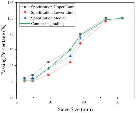
Figure 2.
Combined gradation curve.
2.2.2. Sample Preparation
In this experiment, according to Chinese standard JTG/T F30-2014 [43], the concrete strength grade is designed as C30; the water–cement ratio is 0.46. Three different fly ash contents (5%, 10%, and 15%) and three different sand ratios (32%, 35%, and 38%) were determined. The mix proportions and numbering of the specimens are shown in Table 7.
Table 7.
Concrete mix proportion.
The machine used for concrete mixing was a single-shaft concrete mixer, model HJW-60. The mixing process involved first adding the coarse aggregate along with half of the cement and half of the water, and mixing for 1 min. Then, the remaining fine aggregate, fly ash, cement, and water were added and mixed for an additional 1.5 min. Finally, the mixture was placed into molds. The concrete samples measured 100 mm × 100 mm × 400 mm, as shown in Figure 3. The concrete specimens were cured in a standard curing chamber, model SHBY-60B, at a temperature of 20 °C and a humidity of 95% for 28 days before undergoing the freeze–thaw cycle test.
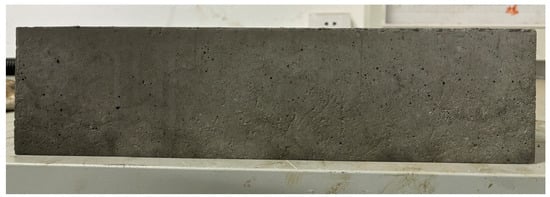
Figure 3.
The concrete specimen.
2.3. Experimental Methods
2.3.1. Freeze–Thaw Cycle Experiment
The freeze–thaw cycle test for the concrete was conducted in accordance with Chinese standard JTG 3420-2020 [44]. After 24 days of curing, the specimens were soaked in water at 20 °C ± 2 °C for 4 days before starting the freeze–thaw cycle test. The rapid freeze–thaw test chamber used in the experiment was the TDR-II model. During the test, the freezing and thawing temperatures were set to −18 °C ± 2 °C and 5 °C ± 2 °C, respectively. Each freeze–thaw cycle took 2 to 5 h to complete, with the thawing time being at least one-quarter of the total freeze–thaw cycle time. The evaluation of frost resistance was based on two indicators: the relative dynamic modulus of elasticity and the mass loss rate. The final result for each test group was determined by averaging the values from three specimens, following the formulas specified in Equations (1) and (2).
where p represents the relative dynamic modulus of elasticity (%) of the specimen after n freeze–thaw cycles, and fn and f0 are the frequency of the horizontal basic frequency (Hz) and the frequency of the frozen–melting resistance test after n times of the frozen–melting cycle.
where W0 is the mass loss rate (%) of the specimen after n freeze–thaw cycles; m0 is the initial mass of the specimen (kg); and m is the mass of the specimen (kg) after n freeze–thaw cycles.
2.3.2. XRD and SEM Testing
A small amount of the concrete specimens was ground into powder, sieved using a 0.075 mm diameter sieve, and then subjected to XRD and SEM testing. The prepared powder samples are shown in Figure 4.

Figure 4.
Samples for XRD and SEM testing.
The XRD testing was conducted using a Bruker D8 X-ray diffractometer, with a scanning range of 5°–90° and a rate of 5°/min.
The SEM testing was performed using an Apreo 2C scanning electron microscope. Due to the poor conductivity of the concrete powder, a gold coating was applied to the surface to prevent image distortion caused by charge accumulation.
3. BP Neural Network-Based Prediction of Mass Loss and Dynamic Elastic Modulus during the Freeze–Thaw Cycle of Manufactured Sand-Cement Concrete
3.1. Test Results and Analysis
The mass loss rate and relative dynamic modulus of elasticity of manufactured sand concrete under various mix proportions are shown in Table 8.
Table 8.
The mass loss rate and relative dynamic modulus of elasticity of manufactured sand concrete under different mix proportions.
3.1.1. Analysis of Mass Loss Rate
Figure 5 and Figure 6 show the mass loss rate curves of manufactured sand concrete. During the first 50 freeze–thaw cycles, the mass loss rate curves of the specimens with various mix proportions changed slightly, and the mass loss rate values were negative. This is partly due to the hydration reaction of the concrete being promoted by water immersion, and partly due to the mass increase caused by water in the internal pores of the concrete freezing in the early stages. However, after 50 freeze–thaw cycles, the freeze–thaw erosion of the specimens intensifies, leading to a rapid increase in the mass loss rate.
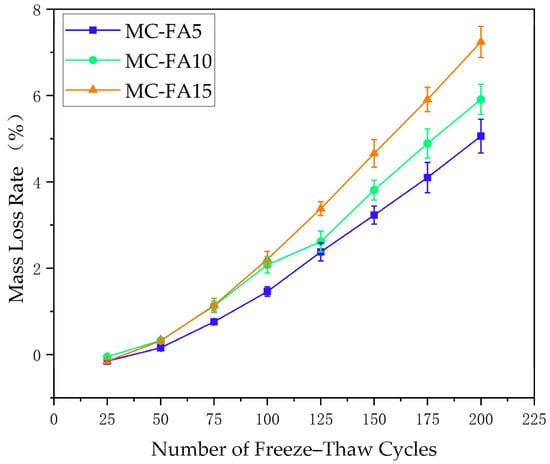
Figure 5.
Relationship between freeze–thaw cycles and mass loss rate under different fly ash contents.
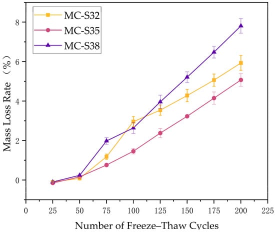
Figure 6.
Relationship between freeze–thaw cycles and mass loss rate under different sand ratios.
From the mass loss rate curves for 200 freeze–thaw cycles with different fly ash contents shown in Figure 5, it is evident that the higher the fly ash content, the faster the increase in the mass loss rate of manufactured sand concrete. After 200 freeze–thaw cycles, the mass loss rates for manufactured sand concrete with 5%, 10%, and 15% fly ash content were 5.06%, 5.91%, and 7.24%, respectively. After 150 freeze–thaw cycles, the mass loss rates for manufactured sand concrete with 5%, 10%, and 15% fly ash content increased by 323%, 237%, and 308%, respectively, compared to the rates after 75 cycles. This indicates that the more freeze–thaw cycles the concrete undergoes, the more severe the freeze–thaw erosion. During the first 50 freeze–thaw cycles, the mass loss of manufactured sand concrete showed almost no difference, indicating that fly ash has little effect on early freeze–thaw resistance. However, after 200 freeze–thaw cycles, there is a significant difference in the mass loss rate, suggesting that fly ash has a substantial impact on the later freeze–thaw erosion of manufactured sand concrete. Yuan et al. [39] set the fly ash content between 0% and 10% and found that the frost resistance of concrete was optimal when the content of fly ash was 6%. However, when the content exceeded 6%, the frost resistance continuously decreased, which is consistent with the results of the aforementioned experiment.
Figure 6 shows the relationship between freeze–thaw cycles and mass loss rate under different sand ratios. As the sand ratio increases, the mass loss rate of manufactured sand concrete decreases initially and then increases. During the first 50 cycles, the influence of the sand ratio on the mass loss rate is similar to the influence of fly ash content. At 75 freeze–thaw cycles, the mass loss rates for manufactured sand concrete with sand ratios of 32%, 35%, and 38% were 1.18%, 0.76%, and 1.98%, respectively. At 150 freeze–thaw cycles, the mass loss rates were 4.28%, 3.23%, and 5.21%, which are 3.62 times, 4.25 times, and 2.63 times the rates at 75 cycles. When the sand ratio is 35%, the concrete has the lowest mass loss rate, with a relatively stable mass loss rate curve and the least degree of freeze–thaw erosion.
3.1.2. Analysis of Relative Dynamic Modulus of Elasticity
From Figure 7, it is quite evident that there is a negative correlation between fly ash content and the relative dynamic modulus of elasticity. The relative dynamic modulus of elasticity curves for manufactured sand concrete with 10% fly ash content were similar to those with 5% fly ash content and higher than those of other comparison groups. The relative dynamic modulus of elasticity for manufactured sand concrete with 5% fly ash content decreases more gradually during the first 75 freeze–thaw cycles, while those with 10%, especially 15% fly ash content, exhibited an almost linear decrease. At 75 freeze–thaw cycles, the relative dynamic modulus of elasticity for manufactured sand concrete with 5%, 10%, and 15% fly ash content was 92.4%, 90.6%, and 83.9%, respectively. By the time 150 freeze–thaw cycles were reached, these values had decreased to 75.1%, 68.3%, and 55.4%, representing decreases of 18.7%, 24.2%, and 33.9%, respectively. This indicated that as the fly ash content increased, the rate of decrease in the relative dynamic modulus of elasticity of manufactured sand concrete accelerated. The conclusions of studies by Yuan [45] and Wang et al. [46] are also similar to the findings mentioned above.

Figure 7.
Relationship between freeze–thaw cycles and relative dynamic modulus of elasticity under different fly ash contents.
From Figure 8, it can be seen that the changes in the relative dynamic modulus of elasticity for manufactured sand concrete, according to the sand ratios from largest to smallest, are 35%, 32%, and 38%. This pattern was consistent with the trend of the mass loss rate. This indicates that in this study, a sand ratio of 35% was the optimal ratio, providing the best dynamic performance for manufactured sand concrete.
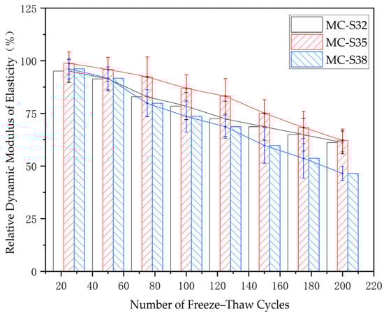
Figure 8.
Relationship between freeze–thaw cycles and relative dynamic modulus of elasticity under different sand ratios.
3.2. Microscopic Analysis of the Freeze–Thaw Resistance of Manufactured Sand Cement Concrete
In Figure 9a, the upper right corner shows fly ash particles, and the microstructure in the image effectively demonstrates the filling effect of fly ash particles. These particles not only fill the voids, improving the density of the concrete, but also react with calcium hydroxide to form C-S-H gel, as shown in Figure 9b. However, previous experiments indicated that as the fly ash content increases, the frost resistance of the concrete decreases. This is because fly ash was added by replacing a portion of the cement, and excessive fly ash can reduce the extent of the cement’s hydration reaction, leading to insufficient C-S-H gel formation, which fails to adequately improve the concrete’s strength and porosity.
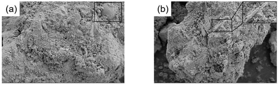
Figure 9.
The microscopic morphology of fly ash concrete at 8000× magnification. (a) fly ash; (b) C-S-H gel.
In Figure 10, it can be observed, via the XRD spectra of concrete with different sand ratios, that the C-S-H gel content at a 38% sand ratio significantly decreased compared to that at a 32% sand ratio. This trend is consistent with the experimental findings discussed in the previous section. C-S-H gel in concrete is crucial for ensuring strength and density. The porosity of the concrete will increase when the content of C-S-H gel is low, leading to moisture retention in the pores, which exacerbates damage caused by freeze–thaw cycles. Moreover, the increase in the peak height representing Ca(OH)2 at a 38% sand ratio can also be observed in the figure. Ca(OH)2 tends to form ice crystals at low temperatures, which increased the internal expansion stress of the concrete, contributing to the decline in its frost resistance.
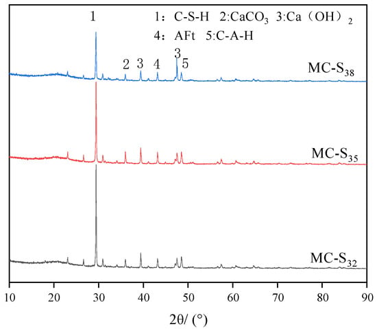
Figure 10.
XRD patterns of manufactured sand cement concrete at different sand ratios.
3.3. Development and Evaluation of a BP Neural Network Prediction Model for Mass Loss and Relative Dynamic Modulus of Elasticity
The data processing steps for the model encompassed defining training and prediction datasets, normalizing the training data, configuring training parameters, and building the BP neural network. This procedure involved training the network, generating predictions, back-normalizing the results, and calculating errors [47].
3.3.1. Select Sample Data
From the 56 sets of mass loss rates obtained after the freeze–thaw cycles, one dataset from each mix proportion was randomly selected as a validation sample, while the remaining 49 sets were used as training samples. The training and validation samples are shown in Table 9 and Table 10.
Table 9.
Selection of training samples.
Table 10.
Selection of validation samples.
3.3.2. Neural Network Training Parameters
Fifteen hidden layers were set during training and the neural network structure is shown in Figure 11. The training results were based on the Levenberg–Marquardt algorithm. A prediction model was obtained after 11 epochs. In the MATLAB (2023 b)command window, the predicted data were obtained by inputting the validation samples selected from Table 10 using the sim function. Finally, function fitting and evaluation metrics such as MSE, RMSE, MAE, and MAPE were used to assess the reliability of the prediction model.
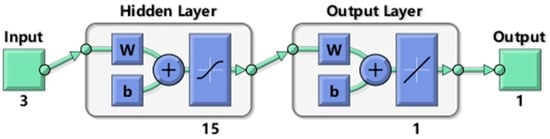
Figure 11.
Neural network structure.
3.3.3. Prediction Results Output
Table 11 shows that the discrepancies between the predicted values from the neural network model and the actual measured values were all below 0.1%, showing minimal error. Thus, this model is reliable for predicting related performance.
Table 11.
Prediction results output.
Similarly, by using the BP neural network to predict the dynamic modulus of elasticity after freeze–thaw cycles, Figure 12 displays the fitting results comparing the actual and predicted values for mass loss rate and dynamic modulus of elasticity.
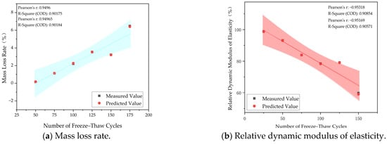
Figure 12.
Fitting results for mass loss rate and relative dynamic modulus of elasticity.
The correlation coefficient of the samples was a crucial metric for assessing the prediction accuracy of the BP neural network. Figure 13 and Figure 14 present the correlation coefficients obtained after model training.
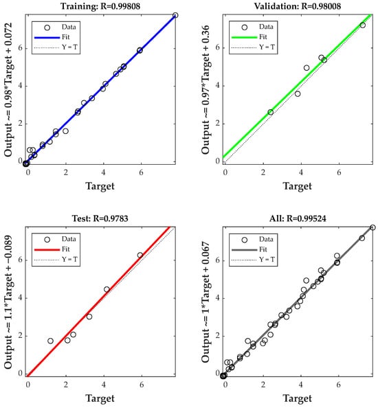
Figure 13.
Correlation coefficient of the BP model for mass loss rate.
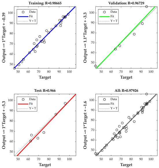
Figure 14.
Correlation coefficient of the BP model for relative dynamic modulus of elasticity.
In Figure 13 and Figure 14, the blue, green, and red lines represent the training set, validation set, and test set of the neural network prediction model, respectively. The R value indicates the prediction performance of each set, with an R value exceeding 0.9 generally signifying a high level of model reliability. From Figure 13 and Figure 14, it can be seen that the correlation coefficients (R) for the mass loss rate and relative dynamic modulus of elasticity prediction models both exceed 0.95. The correlation coefficients for their training samples reached 0.99808 and 0.98665, respectively. Together with the evaluation metrics shown in Table 12, this indicated that the BP neural network prediction models trained in this study have a very high level of reliability.
Table 12.
Evaluation metrics.
4. Conclusions
The study investigated the frost resistance of concrete with varying amounts of manufactured sand and fly ash. The experimental results showed that higher fly ash content led to poorer frost resistance, while the best frost resistance was observed at 35% manufactured sand content. A neural network prediction model was then developed and validated, demonstrating high accuracy and applicability for practical engineering. The specific conclusions are as follows:
- It was found that the incorporation of fly ash into manufactured sand concrete increases the mass loss rate and reduces the relative dynamic modulus of elasticity. At the beginning of the freeze–thaw cycle tests, the manufactured sand concrete begins to experience some freeze–thaw damage. This is because the SiO2 and Al2O3 in fly ash, which can react with the cement hydration products, have relatively low activity. When fly ash replaces part of the cement in the concrete, it cannot generate sufficient hydrated calcium silicate and other hydrated cementitious materials in the early stages of concrete formation. Consequently, the bonding strength between the concrete aggregates decreases. As the number of freeze–thaw cycles increases, under the pressure and infiltration of water, when the external pressure becomes stronger than the internal bonding force, cracks begin to form in the concrete, exacerbating the erosion of the concrete.
- As the sand ratio increases, the freeze–thaw resistance of manufactured sand concrete initially increases and then decreases. This is because an appropriate amount of manufactured sand can effectively fill the voids between the concrete aggregates, thereby improving the freeze–thaw resistance of the concrete. However, an excessive sand ratio will result in too large a surface area of the sand, which hinders the hydration process of the mortar. This reduces the amount of C-S-H gel, a hydration product, thereby decreasing the strength of the concrete mixture and its freeze–thaw resistance. In practical engineering applications, selecting a sand ratio of 35% as a parameter for concrete mix proportioning is a viable option for reference.
- In this study, polynomial fitting was conducted on the mass loss rate and relative dynamic modulus of elasticity of manufactured sand cement concrete after freeze–thaw cycles, and BP neural network prediction models for these two indicators were established. This approach significantly reduces testing costs and time, enhances the accuracy of mix design, and provides a new perspective for exploring the freeze–thaw resistance of manufactured sand cement concrete in the future.
- The various changes in manufactured sand cement concrete during freeze–thaw cycles are a complex process. In this study, the factors influencing the training of the neural network were set as the mix proportion and the number of freeze–thaw cycles. With these limited parameters, good training results have been achieved. Unfortunately, in this study, temperature, humidity, and other factors were not included as variables in the training of the neural network prediction model. Therefore, it is recommended that future research focuses on studying the mechanisms of freeze–thaw damage and increasing the number of influencing factors. This will further improve the model’s accuracy and yield better economic benefits in both experimental and practical engineering applications.
Author Contributions
Conceptualization, Q.G.; methodology, H.W.; software, H.W.; validation, Q.G.; formal analysis, H.W.; investigation, H.W. and Q.G; resources, Q.G.; data curation, H.W.; writing—original draft preparation, H.W.; writing—review and editing, H.W.; visualization, H.W.; supervision, Q.G.; project administration, Q.G.; funding acquisition, H.W. and Q.G. All authors have read and agreed to the published version of the manuscript.
Funding
This study was supported by the National Natural Science Foundation of China (51478288).
Data Availability Statement
All the data are available within the manuscript.
Acknowledgments
We appreciate the Road Engineering Research Center of Suzhou University of Science and Technology for its support.
Conflicts of Interest
The authors declare no conflicts of interest.
References
- Akhtar, M.N.; Bani-Hani, K.A.; Malkawi, D.A.H.; Albatayneh, O. Suitability of sustainable sand for concrete manufacturing—A complete review of recycled and desert sand substitution. Results Eng. 2024, 23, 102478. [Google Scholar] [CrossRef]
- Guo, S.; Ding, Y.; Zhang, X.; Xu, P.; Bao, J.; Zou, C. Tensile properties of steel fiber reinforced recycled concrete under bending and uniaxial tensile tests. J. Build. Eng. 2024, 96, 110467. [Google Scholar] [CrossRef]
- Cao, J.; Tu, N.; Liu, T.; Han, Z.; Tu, B.; Zhou, Y. Prediction models for creep and creep recovery of fly ash concrete. Constr. Build. Mater. 2024, 428, 136398. [Google Scholar] [CrossRef]
- Wu, B.; Yang, L.; Mei, Y.; Sun, Y.; Shen, J. Dynamic Tensile Properties of Straw fiber Reinforced Rubber Concrete. J. Build. Eng. 2024, 96, 110455. [Google Scholar] [CrossRef]
- Yang, H.; Jiao, Y.; Xing, J.; Liu, Z. Statistical model and fracture behavior of manufactured sand concrete with varying replacement rates and stone powder contents. J. Build. Eng. 2024, 95, 110102. [Google Scholar] [CrossRef]
- Raman, S.N.; Ngo, T.; Mendis, P.; Mahmud, H.B. High-strength rice husk ash concrete incorporating quarry dust as a partial substitute for sand. Constr. Build. Mater. 2011, 25, 3123–3130. [Google Scholar] [CrossRef]
- Miao, G.; Zhou, A.; Xue, C.; Yang, Y.; Qiao, H.; Su, L. Study on gas transport characteristics of manufactured sand concrete and modeling of random hierarchical bundle based on pore structure. J. Build. Eng. 2024, 96, 110388. [Google Scholar] [CrossRef]
- Ma, R.; Zhang, L.; Song, Y.; Lin, G.; Qian, X.; Qian, K. Recycling stone powder as a partial substitute for cementitious materials into eco-friendly manufactured sand ultra-high performance concretes: Towards cleaner and more cost-effective construction production. J. Build. Eng. 2024, 92, 109772. [Google Scholar] [CrossRef]
- Jadhav, P. An Experimental Investigation on the Properties of Concrete Containing Manufactured Sand. Int. J. Adv. Eng. Technol. 2012, 3, 101–104. [Google Scholar]
- Meng, Q.; Jing, X.; Wang, H.; Guo, X.; Song, J.; Du, J. Flexural fatigue properties of concrete based on different replacement percentage of natural sand with manufactured sand. J. Build. Eng. 2024, 87, 108987. [Google Scholar] [CrossRef]
- Soleimani, T.; Hayek, M.; Junqua, G.; Salgues, M.; Souche, J.-C. Environmental, economic and experimental assessment of the valorization of dredged sediment through sand substitution in concrete. Sci. Total Environ. 2023, 858, 159980. [Google Scholar] [CrossRef] [PubMed]
- Attri, G.K.; Gupta, R.C.; Shrivastava, S. Comparative Environmental Impacts of Recycled Concrete Aggregate and Manufactured Sand Production. Process Integr. Optim. Sustain. 2022, 6, 737–749. [Google Scholar] [CrossRef]
- Bahraq, A.A.; Jose, J.; Shameem, M.; Maslehuddin, M. A review on treatment techniques to improve the durability of recycled aggregate concrete: Enhancement mechanisms, performance and cost analysis. J. Build. Eng. 2022, 55, 104713. [Google Scholar] [CrossRef]
- Singh, S.; Nagar, R.; Agrawal, V. A review on Properties of Sustainable Concrete using granite dust as replacement for river sand. J. Clean. Prod. 2016, 126, 74–87. [Google Scholar] [CrossRef]
- Shen, W.; Wu, J.; Du, X.; Li, Z.; Wu, D.; Sun, J.; Wang, Z.; Huo, X.; Zhao, D. Cleaner production of high-quality manufactured sand and ecological utilization of recycled stone powder in concrete. J. Clean. Prod. 2022, 375, 134146. [Google Scholar] [CrossRef]
- Xia, J.; Chen, K.; Wu, Y.; Xiao, W.; Jin, W.; Zhang, J. Shear fatigue behavior of reinforced concrete beams produced with manufactured sand as alternatives for natural sand. J. Build. Eng. 2022, 62, 105412. [Google Scholar] [CrossRef]
- Li, B.; Ke, G.; Zhou, M. Influence of manufactured sand characteristics on strength and abrasion resistance of pavement cement concrete. Constr. Build. Mater. 2011, 25, 3849–3853. [Google Scholar] [CrossRef]
- Shen, W.; Liu, Y.; Cao, L.; Huo, X.; Yang, Z.; Zhou, C.; He, P.; Lu, Z. Mixing design and microstructure of ultra high strength concrete with manufactured sand. Constr. Build. Mater. 2017, 143, 312–321. [Google Scholar] [CrossRef]
- Li, B.; Wang, J.; Zhou, M. Effect of limestone fines content in manufactured sand on durability of low- and high-strength concretes. Constr. Build. Mater. 2009, 23, 2846–2850. [Google Scholar] [CrossRef]
- Altuki, R.; Tyler Ley, M.; Cook, D.; Jagan Gudimettla, M.; Praul, M. Increasing sustainable aggregate usage in concrete by quantifying the shape and gradation of manufactured sand. Constr. Build. Mater. 2022, 321, 125593. [Google Scholar] [CrossRef]
- Nanthagopalan, P.; Santhanam, M. Fresh and hardened properties of self-compacting concrete produced with manufactured sand. Cem. Concr. Compos. 2011, 33, 353–358. [Google Scholar] [CrossRef]
- Cai, B.; Chen, H.; Xu, Y.; Fan, C.; Li, H.; Liu, D. Study on fracture characteristics of steel fiber reinforced manufactured sand concrete using DIC technique. Case Stud. Constr. Mater. 2024, 20, e03200. [Google Scholar] [CrossRef]
- Wang, Z.; Li, H.; Huang, F.; Yang, Z.; Wen, J.; Yi, Z. Bond properties between railway high-strength manufactured sand concrete and steel bars. Constr. Build. Mater. 2024, 416, 135179. [Google Scholar] [CrossRef]
- Zhu, X.; Zhang, Y.; Liu, Z.; Qiao, H.; Ye, F.; Lei, Z. Research on carbon emission reduction of manufactured sand concrete based on compressive strength. Constr. Build. Mater. 2023, 403, 133101. [Google Scholar] [CrossRef]
- Wang, X.; Wang, F.; Liu, X.; Zhu, P.; Liu, H.; Chen, C. Study on the high temperature performance of recycled concrete with manufactured sand. J. Build. Eng. 2024, 91, 109479. [Google Scholar] [CrossRef]
- Yang, X.; Pan, M.; Zheng, S.; Liang, J.; Tan, M.; Rong, H. Influence of stone dust content on carbonation performance of manufactured sand concrete (MSC). J. Build. Eng. 2023, 76, 107341. [Google Scholar] [CrossRef]
- Han, Z.; Zhang, Y.; Qiao, H.; Feng, Q.; Xue, C.; Shang, M. Study on axial compressive behavior and damage constitutive model of manufactured sand concrete based on fluidity optimization. Constr. Build. Mater. 2022, 345, 128176. [Google Scholar] [CrossRef]
- Smarzewski, P.; Barnat-Hunek, D. Mechanical and durability related properties of high performance concrete made with coal cinder and waste foundry sand. Constr. Build. Mater. 2016, 121, 9–17. [Google Scholar] [CrossRef]
- Shi, H.; Wang, H.; Xue, S.; Feng, S.; Li, Y. Durability evaluation of iron tailings concrete under freeze-thaw cycles and sulfate erosion based on entropy weighting method. Constr. Build. Mater. 2024, 443, 137747. [Google Scholar] [CrossRef]
- Jafari, A.; Ma, L.; Shahmansouri, A.A.; Dugnani, R. Quantitative fractography for brittle fracture via multilayer perceptron neural network. Eng. Fract. Mech. 2023, 291, 109545. [Google Scholar] [CrossRef]
- Wu, Y.C.; Feng, J.W. Development and Application of Artificial Neural Network. Wirel. Pers. Commun. 2018, 102, 1645–1656. [Google Scholar] [CrossRef]
- Bahrami, S.; Alamdari, S.; Farajmashaei, M.; Behbahani, M.; Jamshidi, S.; Bahrami, B. Application of artificial neural network to multiphase flow metering: A review. Flow Meas. Instrum. 2024, 97, 102601. [Google Scholar] [CrossRef]
- Zhao, Y.; Hu, H.; Song, C.; Wang, Z. Predicting compressive strength of manufactured-sand concrete using conventional and metaheuristic-tuned artificial neural network. Measurement 2022, 194, 110993. [Google Scholar] [CrossRef]
- Tian, H.; Qiao, H.; Zhang, Y.; Feng, Q.; Wang, P.; Xie, X. Predicting the impermeability and mechanical properties of manufactured sand polymer waterproof mortar using an optimised back-propagation neural network. Constr. Build. Mater. 2024, 441, 137475. [Google Scholar] [CrossRef]
- Sharma, H.; Ahmad Khan, R. Predicting the mechanical properties of spent foundry sand concrete (SFSC) using artificial neural network (ANN). Mater. Today Proc. 2023, 93, 287–295. [Google Scholar] [CrossRef]
- Skare, E.L.; Sheiati, S.; Cepuritis, R.; Mørtsell, E.; Smeplass, S.; Spangenberg, J.; Jacobsen, S. Rheology modelling of cement paste with manufactured sand and silica fume: Comparing suspension models with artificial neural network predictions. Constr. Build. Mater. 2022, 317, 126114. [Google Scholar] [CrossRef]
- Mehta, V. Machine learning approach for predicting concrete compressive, splitting tensile, and flexural strength with waste foundry sand. J. Build. Eng. 2023, 70, 106363. [Google Scholar] [CrossRef]
- Santosh Kumar, G.; Rajasekhar, K. Performance analysis of Levenberg-Marquardt and Steepest Descent algorithms based ANN to predict compressive strength of SIFCON using manufactured sand. Eng. Sci. Technol. Int. J. 2017, 20, 1396–1405. [Google Scholar] [CrossRef]
- GB175-2023; General Portland Cement. Ministry of Industry and Information Technology of China: Beijing, China, 2023. (In Chinese)
- JTG 3432-2024; Test Procedures for Highway Engineering Aggregates. Ministry of Transport of the People’s Republic of China: Beijing, China, 2024. (In Chinese)
- GB/T1596-2017; F1y Ash Used for Cememt and Concrete. General Administration of Quality Supervision, Inspection and Quarantine of the People’s Republic of China: Beijing, China, 2017. (In Chinese)
- GB/T 14684-2022; Construction Sand. State Administration for Market Regulation of China: Beijing, China, 2022. (In Chinese)
- JTG/T F30-2014; Technical Specifications for Highway Cement Concrete Pavement Construction. Ministry of Transport of the People’s Republic of China: Beijing, China, 2014. (In Chinese)
- JTG 3420-2020; Test Procedures for Highway Engineering Cement and Cement Concrete. Ministry of Transport of the People’s Republic of China: Beijing, China, 2020. (In Chinese)
- Yuan, S.; Li, K.; Luo, J.; Yin, W.; Chen, P.; Dong, J.; Liang, W.; Zhu, Z.; Tang, Z. Research on the frost resistance performance of fully recycled pervious concrete reinforced with fly ash and basalt fiber. J. Build. Eng. 2024, 86, 108792. [Google Scholar] [CrossRef]
- Wang, D.; Zhou, X.; Meng, Y.; Chen, Z. Durability of concrete containing fly ash and silica fume against combined freezing-thawing and sulfate attack. Constr. Build. Mater. 2017, 147, 398–406. [Google Scholar] [CrossRef]
- Wu, H.; Xu, F.; Li, B.; Gao, Q. Study on Expansion Rate of Steel Slag Cement-Stabilized Macadam Based on BP Neural Network. Materials 2024, 17, 3558. [Google Scholar] [CrossRef] [PubMed]
Disclaimer/Publisher’s Note: The statements, opinions and data contained in all publications are solely those of the individual author(s) and contributor(s) and not of MDPI and/or the editor(s). MDPI and/or the editor(s) disclaim responsibility for any injury to people or property resulting from any ideas, methods, instructions or products referred to in the content. |
© 2024 by the authors. Licensee MDPI, Basel, Switzerland. This article is an open access article distributed under the terms and conditions of the Creative Commons Attribution (CC BY) license (https://creativecommons.org/licenses/by/4.0/).