Article

Optimising Plate Thickness in Interlocking Inter-Module Connections for Modular Steel Buildings: A Finite Element and Random Forest Approach

Department of Civil Engineering, Faculty of Engineering and Built Environment, Universiti Kebangsaan Malaysia (UKM), Bangi 43600, Malaysia
*
Authors to whom correspondence should be addressed.
Buildings 2024, 14(5), 1254; https://doi.org/10.3390/buildings14051254
Submission received: 26 March 2024 / Revised: 23 April 2024 / Accepted: 24 April 2024 / Published: 29 April 2024
(This article belongs to the Section Building Structures)

Abstract

:
Interlocking Inter-Module Connections (IMCs) in Modular Steel Buildings (MSBs) have garnered significant interest from researchers. Despite this, the optimisation of plate thicknesses in such structures has yet to be extensively explored in the existing literature. Therefore, this paper focuses on optimising the thickness of interlocking IMCs in MSBs by leveraging established experimental and numerical simulation methodologies. The study developed various numerical models for IMCs with plate thicknesses of 4 mm, 6 mm, 10 mm, and 12 mm, all subjected to compression loading conditions. The novelty of this study lies in its comprehensive parametric analysis, which evaluates the slip prediction model. A random forest regression model, trained using the ‘TreeBagger’ function, was also implemented to predict slip values based on applied force. Sensitivity analysis and comparisons with alternative methods underscored the reliability and applicability of the findings. The results indicate that a plate thickness of 11.03 mm is optimal for interlocking IMCs in MSBs, achieving up to 8.08% in material cost reductions while increasing deformation resistance by up to 50.75%. The ‘TreeBagger’ random forest regression significantly enhanced slip prediction accuracy by up to 7% at higher force levels.

1. Introduction

Modular Steel Buildings (MSBs) have become increasingly popular in the construction industry due to their numerous advantages, including cost-effectiveness, speed of construction period, and flexibility. Modular buildings are built upon the Lego matter construction approach, in which their components (modules) are fabricated in industrial units (off-site) in a factory-controlled environment system based on the customer’s request and then transferred and assembled at the construction site (on-site) in a desired configuration to form an entire building [1,2,3,4,5,6,7]. Compared to the traditional on-site technique, the entire modular building’s on-site construction time is limited to assembly modules with suitable Inter-Module Connections (IMCs). The suitable IMCs must ensure the overall stability and strength of the building, capable of withstanding loads and stresses from various sources (wind, seismic activity, and weight of the building itself); the connections should accommodate the modular nature of the building, allowing easy assembly and disassembly [8,9,10]. Given the prefabricated nature of modules, connections should be designed with tolerances that account for light variations in fabrication. Ideal connections should also allow for reuse or recycling.
Modular steel buildings are severely impacted by choosing suitable IMCs, especially in multi-storey MSBs, when the primary load path for transferring forces between modules comprises IMCs [11]. From a structural viewpoint, IMCs are crucial since they affect the overall stability of modular steel buildings [12,13,14]. As the on-site construction process is limited to connecting the modules, IMCs are highly susceptible to variables such as skilled labour, environmental conditions, availability of suitable equipment, etc. [15]. Since modular building is a new kind of construction in terms of research and industrial practices, the main practical challenge is ensuring the safety and longevity of these structures by ensuring a complete connection between their modules.
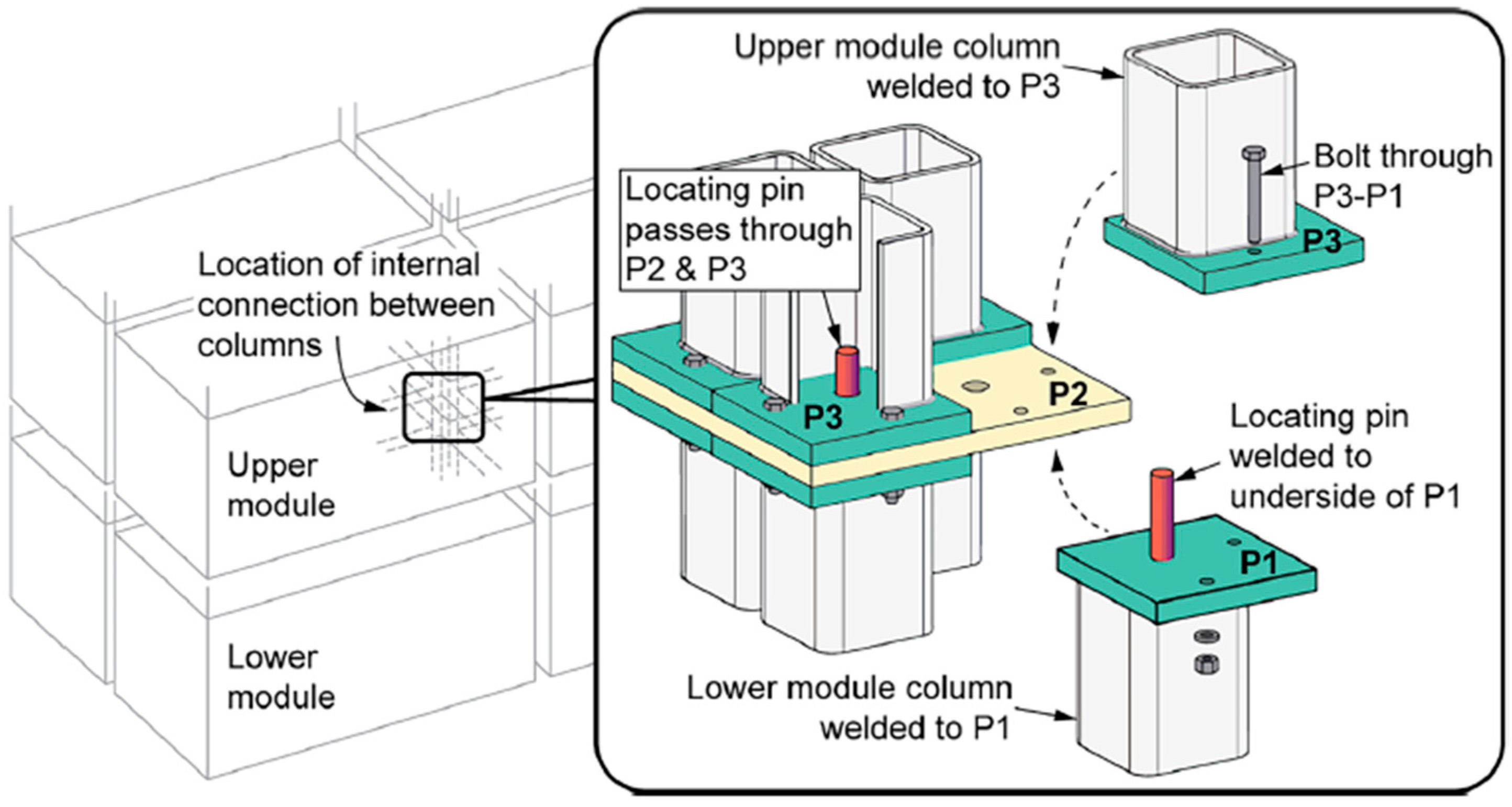
Researchers and engineers have recently paid more attention to modular buildings’ IMCs. Extensive state-of-the-art literature studies on the structural performance of IMCs were conducted in [8,11,14,16,17,18,19,20,21,22,23,24,25,26,27,28,29,30,31,32,33,34,35]. While the internal area between the adjacent modules is still the most prone, various (internal) inter-module connection techniques have been proposed in the available literature that aim for easy and fast installations using bolted shear keys, plates, grouts, etc. [10,28,36,37,38,39,40,41,42,43,44,45]. Generally, the two forms of IMCs are horizontal and vertical connections, where the floor beams of the upper modules and the ceiling beams of the lower modules are connected horizontally; the vertical connection for corner support modules involves joining the upper module to the lower module at the corner columns. Corfar et al. [46] classified the IMCs into three main groups, as shown in Figure 1. The most common method for connecting the top and lower modules involves shear keys with gusset plates or fastened gusset plates [47,48]. Lacey et al. [20] introduced an adapted connection that combined bolt-and-plate connections with the interlocking action of pins, as shown in Figure 2. In contrast, the pre-welded locating pins improved the site installation of units; significant slippage was inflicted upon the connection due to the manufacturing tolerances in the bolt and pin holes.
The interlocking mechanism allows for quicker assembly and disassembly of modules, which is crucial for modular buildings. Also, those connections can provide significant strength and stability, disturbing loads effectively across the structures as they are fabricated with high precision. Interlocking (IMCs) can accommodate manufacturing tolerances, ensuring a tight and secure fit between the modules. Interlocking designs may reduce the need for welding on-site, thereby reducing construction time, labour costs, and potential points of weakness, as a tight fit is ensured between the modules, they can be designed to be visually appealing or completely hidden, maintaining the architectural integrity of the modular building [19,20,49]. The ease of disassembly and reassembly support the rescue of modules in different configurations or locations, aligning with sustainable construction practices by reducing waste and demand for new materials. Yet they raise questions regarding the accommodation of installation tolerances without compressing the slip (deformation) precautions [20,44]. This ambiguity underscores the importance of further research in this area; in this context, the choice of plate thickness for interlocking (IMCs) is pivotal as it directly influences the connection’s ability to distribute stresses and resistance deformation under load.
Typically, IMCs are investigated using experimental programmes, and their outcomes verified using analytical and numerical research data [7,20,34,50,51,52,53,54,55,56,57,58]. The only approaches that can be used to investigate the impact of the interlocking (IMCs) plate thickness are experimental programmers and numerical simulation using the Finite Element (FE) methods [59,60,61,62,63,64]. Those approaches have not addressed the optimum plate thickness for interlocking (IMCs) well. With a reasonable material model and effective modelling techniques, the FE method has emerged as the primary analysis tool for predicting the behaviour of IMCs under various loading conditions.
To overcome the drawbacks of investigating the optimum interlocking (IMCs) plate thickness, comprehensive research on the analysis of plate thickness and structural integrity of interlocking (IMCs) was conducted in this work and since the FE model is more cost-effective than experimental programmes, an FE model was built upon to extend the foundational work of Lacey et al. [20]. While the Lacey et al. [20] work focused on a three-plate (SP14, SP15, and SP16) connection model with a uniform thickness of 8 mm, this study introduces novel contributions by investigating the variations in plate thickness (4, 6, 10, and 12 mm) and conducting non-linear analysis under same compression loading AGS-300kNX Universal Test Machine (UTM) conditions used by Lacey et al. [20], using ANSYS 2023R2 [65] software. Further, the study expands the scope of the analysis by incorporating connection stiffness behaviour into the study evaluation. The FE models then served as a basis for the groundbreaking parametric analysis conducted with MATLAB R2022b [66], aimed to examine the slip phenomenal occurrence in the connection through various study approaches, including polynomial formulas. This introduces a novel slip (deformation) prediction model and validates it against empirical data from previous studies. Moreover, this research pioneers innovative static and random forest regression techniques, specifically employing the ‘TreeBagger’ function to train a random forest regression model for predicting slip value based on applied force. This represents a significant expansion of the methodological toolkit for analysing IMCs.
The study also introduces a comprehensive sensitivity analysis, a step forward in identifying errors and anomalies and comparing the results with alternative methods (linear regression analysis and anomaly detection) and introduces a single-objective optimisation model where its goal is to maximise a composite measure of interlocking (IMCs) plate material properties against economic cost. This paper is organised as follows: Section 2 describes the methodology, focusing on modelling methods and plate thickness optimisation. Section 3 presents the results from the FE analysis and discusses the findings. Section 4 advances predictive modelling studies, employing polynomial regression and random forest regression techniques. Section 5 delves into advanced predictive modelling, exploring the impact of plate thickness variations on stiffness characteristics through sensitivity analysis and anomaly detection, concluding with a comprehensive optimisation of IMC plate thickness that integrates material property analysis with cost-efficiency evaluation. Finally, Section 6 wraps up with the conclusion, highlighting the implications of the findings.

2. Modelling Methods and Optimising (IMCs) Plate Thickness

2.1. Connection Configuration and Properties

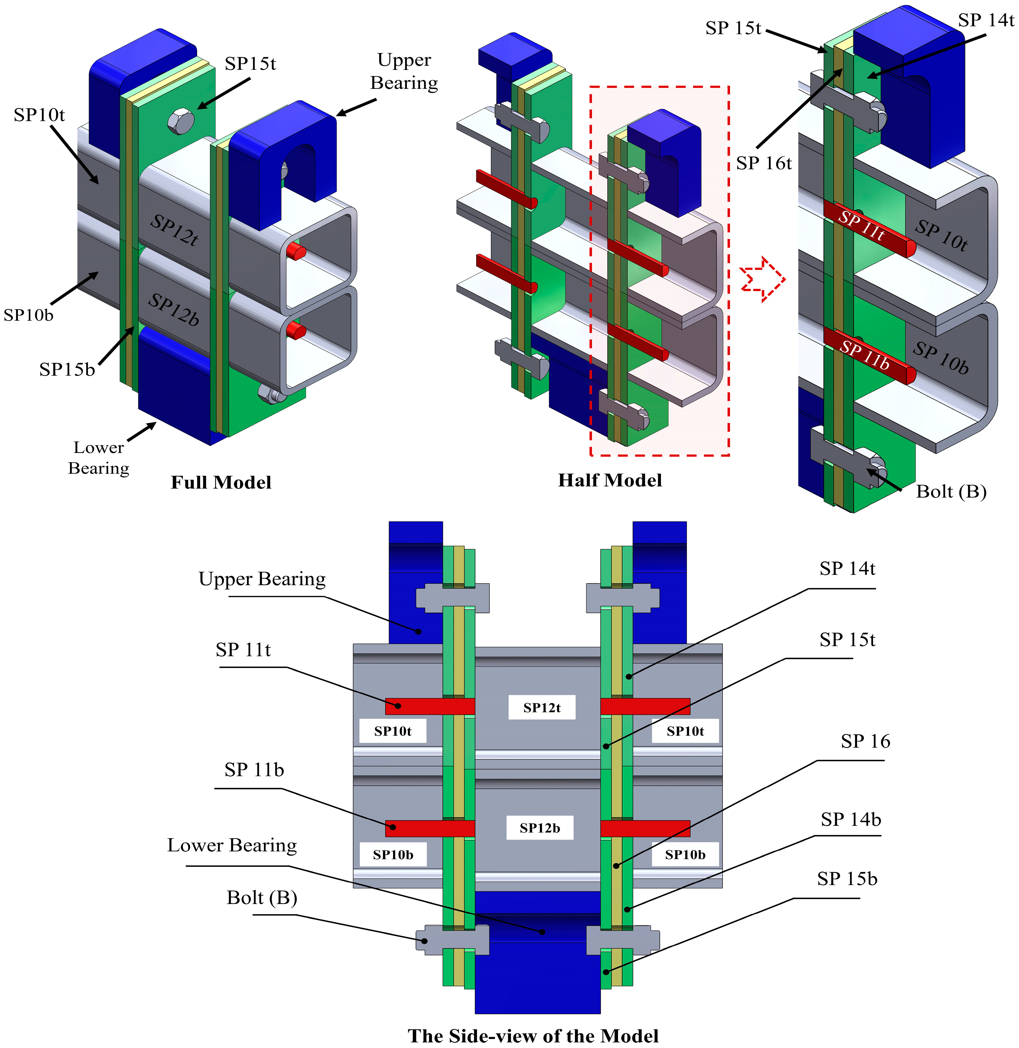
Inter-module connections (IMCs) are critical because they maintain the modular building’s structural robustness and general stability [10,67]. Similarly to the Lacey et al. [20] work, the plates are labelled (SP14, SP15, and SP16) for convenience in the following discussion where (SP) refers to Single Plate, (t) and (b) refer to the top and bottom of the assembled specimen. Their study selected sample (A) as the control model for this study and labelled it as (A0). The connection design focused on the interplay between (SP14, SP15, and SP16); the connection geometry shown in Figure 3 captures the full and cut-way view to present the hidden connection components and the connection dimensions specified in Table 1.
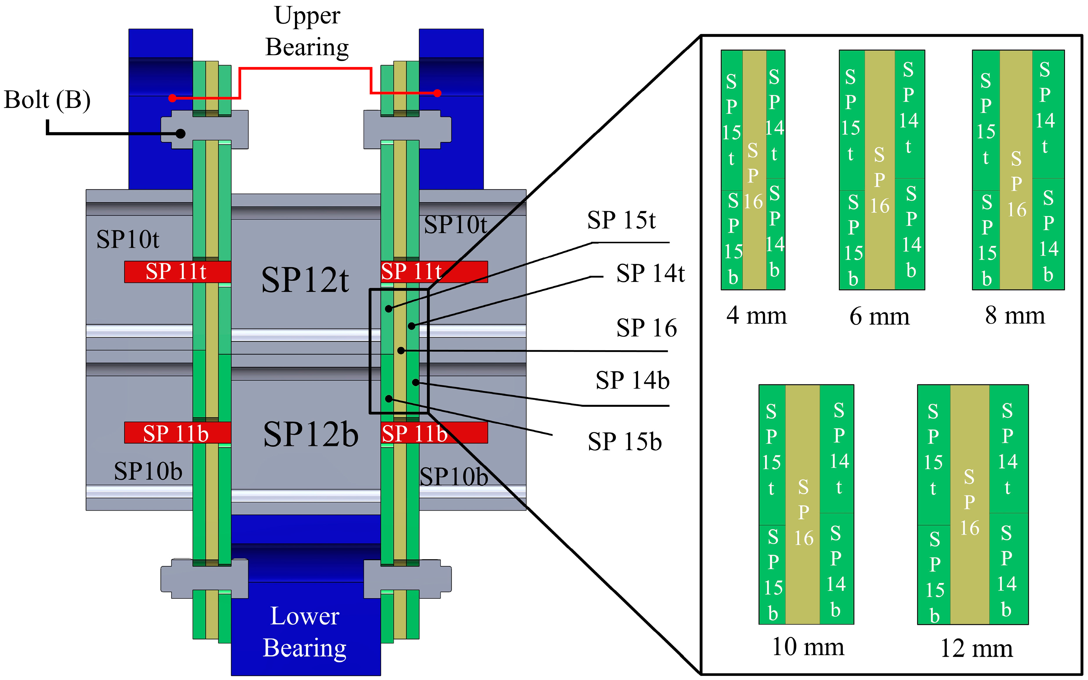
The material properties of the connection are selected to meet stringent industry standards, emphasising specific criteria for strength and durability, as shown in Table 2. The variations in the connection plate thickness are shown in Table 3. Each plate type was evaluated through a series of cases starting with (A0) representing the controller model, (A1) to (A4) presenting the proposed cases, with interlocking (IMCs) plate thickness ranging from 4.0 mm to 12.0 mm, as shown in Figure 4.

2.2. Compression Loading (UTM) Test Conditions Modelling

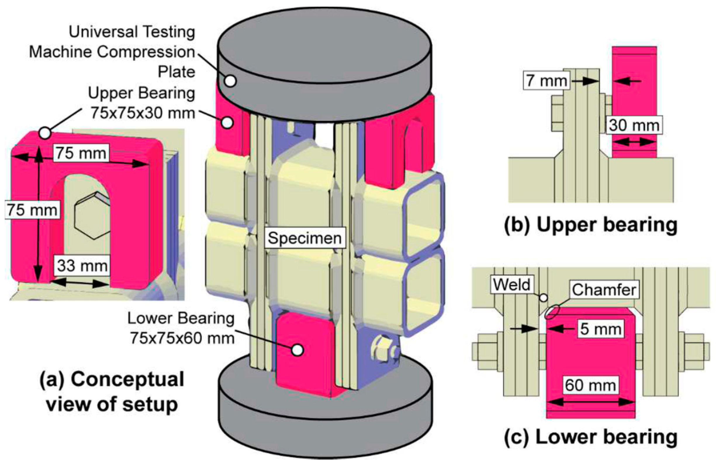
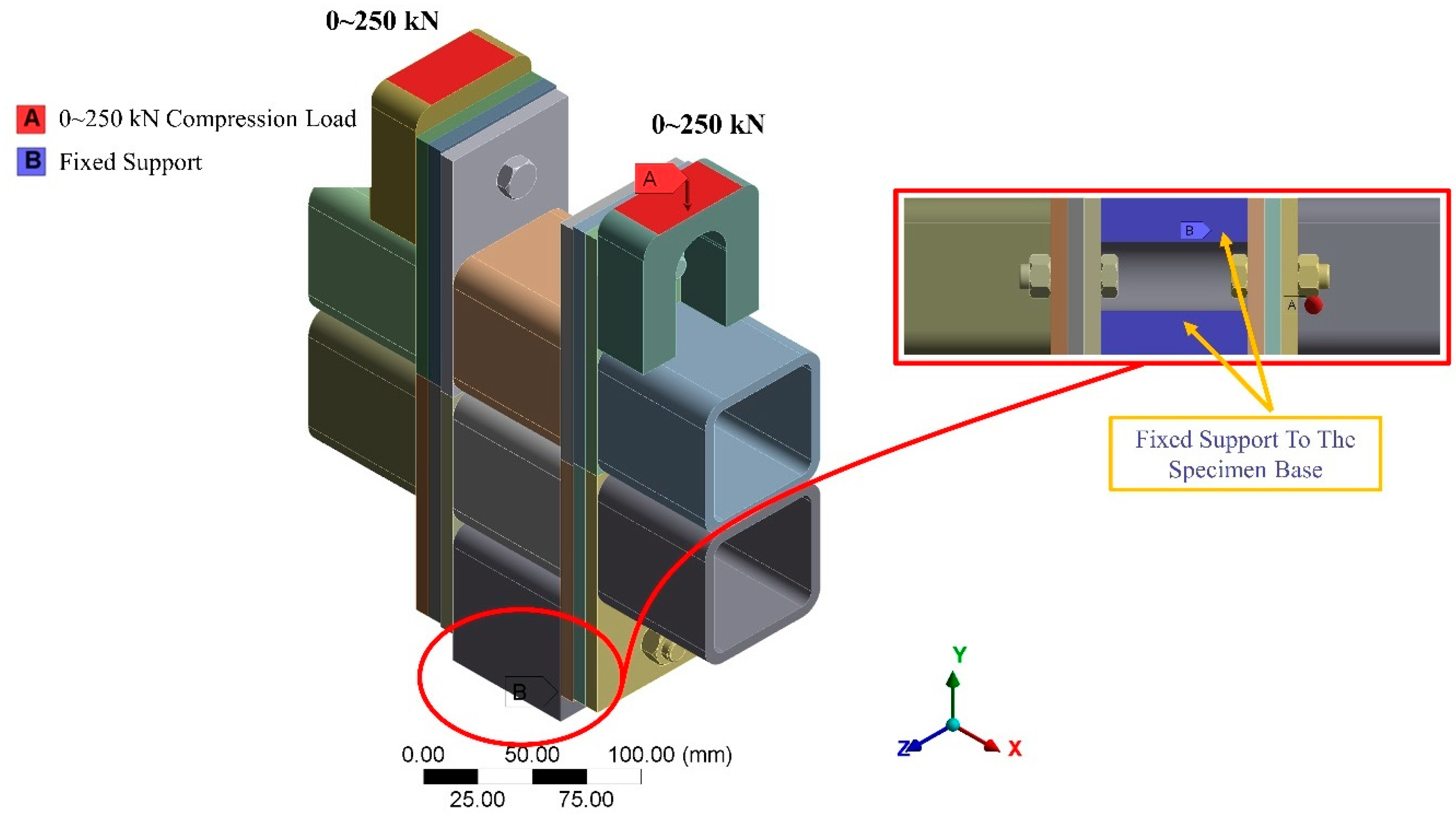
To re-apply the same compression loading AGS-300kNX Universal Test Machine (UTM) conditions of the practical experience in ANSYS 2023R2 software, an FE method was adopted. In the previous study, Lacey et al. [20] sample (A) was modelled using ABAQUS version 6.14 software by applying (UTM) test loading conditions with loads ranging from 0 to 250 kN at a rate of 0.1 kN/s (refer to Figure 5); the previous FE model was employed with 8-node linear brick elements with reduced integration (CSD8R). This choice was informed by the need to address the significant validation error of over 95.62% observed between numerical and experimental results in the previous study, as illustrated in Figure 6. The selection of (CSD8R) elements over other types was crucial due to their superior performance in handling the complex interactions typical in modular connection simulations, such as avoiding shear locking and better-managing pressure conditions. Subsequently, this study re-applied the exact compression loading conditions in ANSYS 2023R2 software, mirroring the original test setup by applying a compression load within the range of 0 to 250 kN in the negative Y-axis direction and ensuring fixed support to the specimen base, as depicted in Figure 7.

2.3. Interlocking Connection Modelling

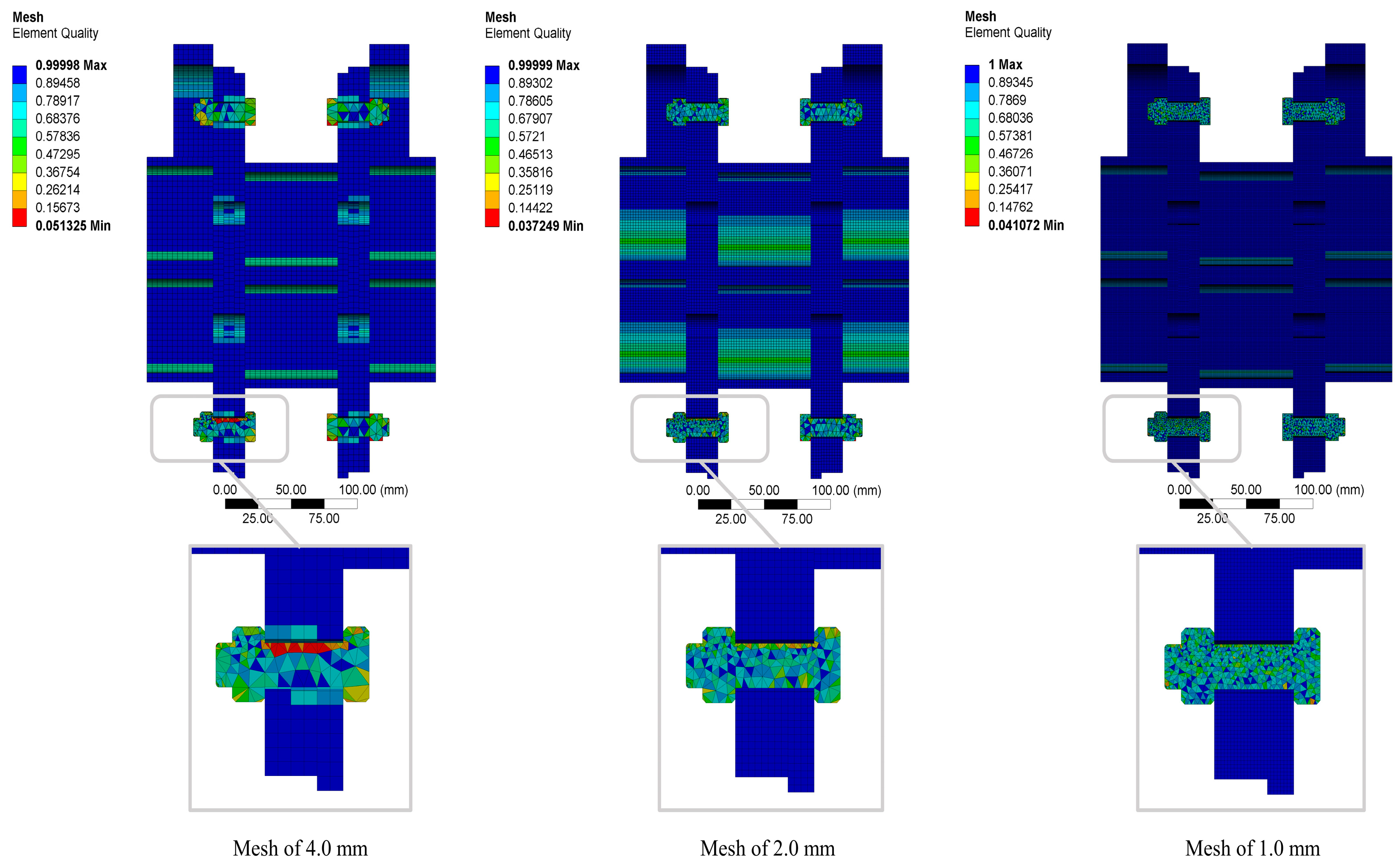
To investigate the accuracy of the optimum interlocking (IMCs) plate thickness numerically, FE models with various plate thicknesses of 4, 6, 10, and 12 mm (refer to Table 3) were developed in ANSYS 2023R2, as shown in Figure 4, based on the experimental approach presented by Lacey et al. [20]. The geometric properties of the connection cases were defined in the FE model following Table 1 and their material specifications were defined following Table 2. The models were subjected to a selected mesh element size of 1.0 mm, 2.0 mm, and 4.0 mm with a growth rate set at 1.2. To balance an accurate and efficient FE model, a middle range of detail (coarse) at the centre of the span angle, added initial size seeds to the assembly, with the error limits being more aggressive, allowing for a maximum of five mesh layers as shown in Figure 8. The choice of constant mesh sizes over adaptive meshes was critical in ensuring direct comparability across simulations and maintaining computational efficiency to ensure any observed differences were attributable solely to plate thickness variations. A mesh size of 1.0 mm reaches the maximum mesh quality of 25.31% compared to 2.0 mm and 4.0 mm. To validate the accuracy of the FE model, Figure 6 shows the comparative analysis between the force-slip Lacey et al. [20] experimental approach results and the FE model mesh size results; validation results reveal that the validation error between the FE model results and the experimental results was 2.13%, which was more accurate, 95.63%, than the previous study FE results. This study therefore adopted 1.0 m elements mesh size though all the FE modelling.

2.4. Optimising Interlocking (IMCs) Plate Thickness

The study utilised a single objective optimisation model to optimise the plate thickness for interlocking (IMCs) in modular steel buildings. The proposed single objective optimisation approach (refer to Appendix A) combines multiple factors (yield and tensile strengths relative to cost) into one creation; the choice of single objective optimisation allows for a clear focus on one main goal, making it easier to measure and compare results. The 1st stage involved defining the minimum yield stress of 360 MPa and tensile strength of 450 Mpa for G350 steel. In the 2nd stage, the span length (L) was specified in meters, which might be relevant for structural application. However, it is not used in the proposed model script and indicates the cost (C) per millimetre of material thickness. The 3rd stage generated a linear space array of 100 values ranging from 4 mm to 12 mm plate thickness. The 4th stage involved the following: using a computational loop for each thickness in the defined range by converting thickness from meters to millimetres, calculating the yield and tensile strengths by normalising the strength of the material based on the ratio of the current thickness to baseline (4 mm plate thickness in this case), computing the cost values as the product of the cost per millimetres and the thickness, and determining efficiency values as the ratio of the sum of yield and tensile strengths to the cost for each thickness.

3. FE Results & Discussion

3.1. Slip (Deformation) Behaviour

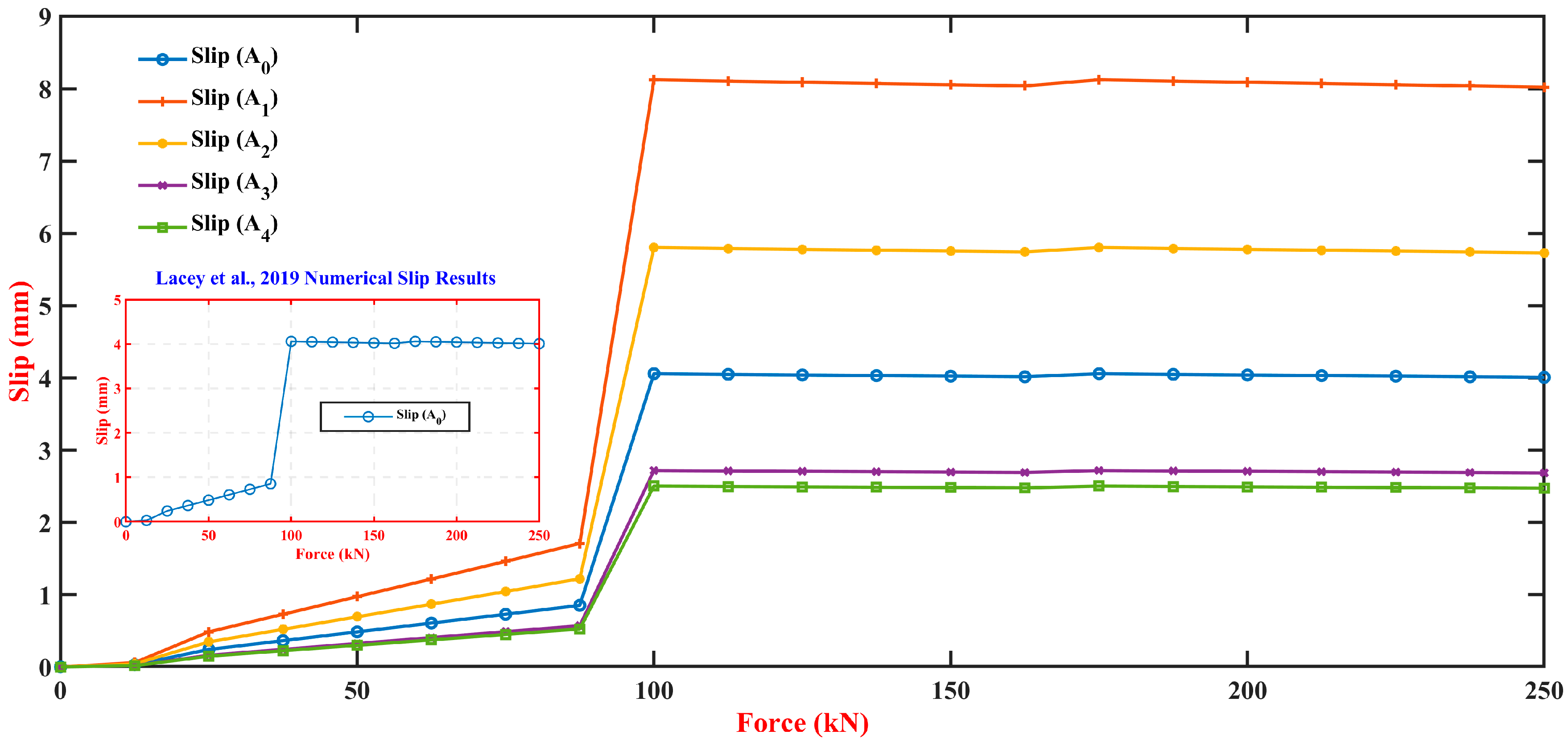
The examined slip (deformation) across the interlocking (IMCs) plate thickness scenarios (A0 through A4) are shown in Figure 9. The analysis reveals that the controller model (A0) exhibits an increased slip with the applied force, reaching a slip of 4.0 mm at 250 kN. Notably, compared to case (A1), which exhibits a slip increase peaking up to 8.02 mm at the same applied force, this emphasises the heightened susceptibility to slip in thinner plates. Case (A2), with an intermediate plate thickness, shows an elevated slip behaviour less than (A1). (A3) and (A4) cases demonstrated a notable reduction in slip, with (A4), the thickest plate, exhibiting a 2.46 mm slip at 250 kN force, which has a reduction of ≈38% from the controlled model (A0).
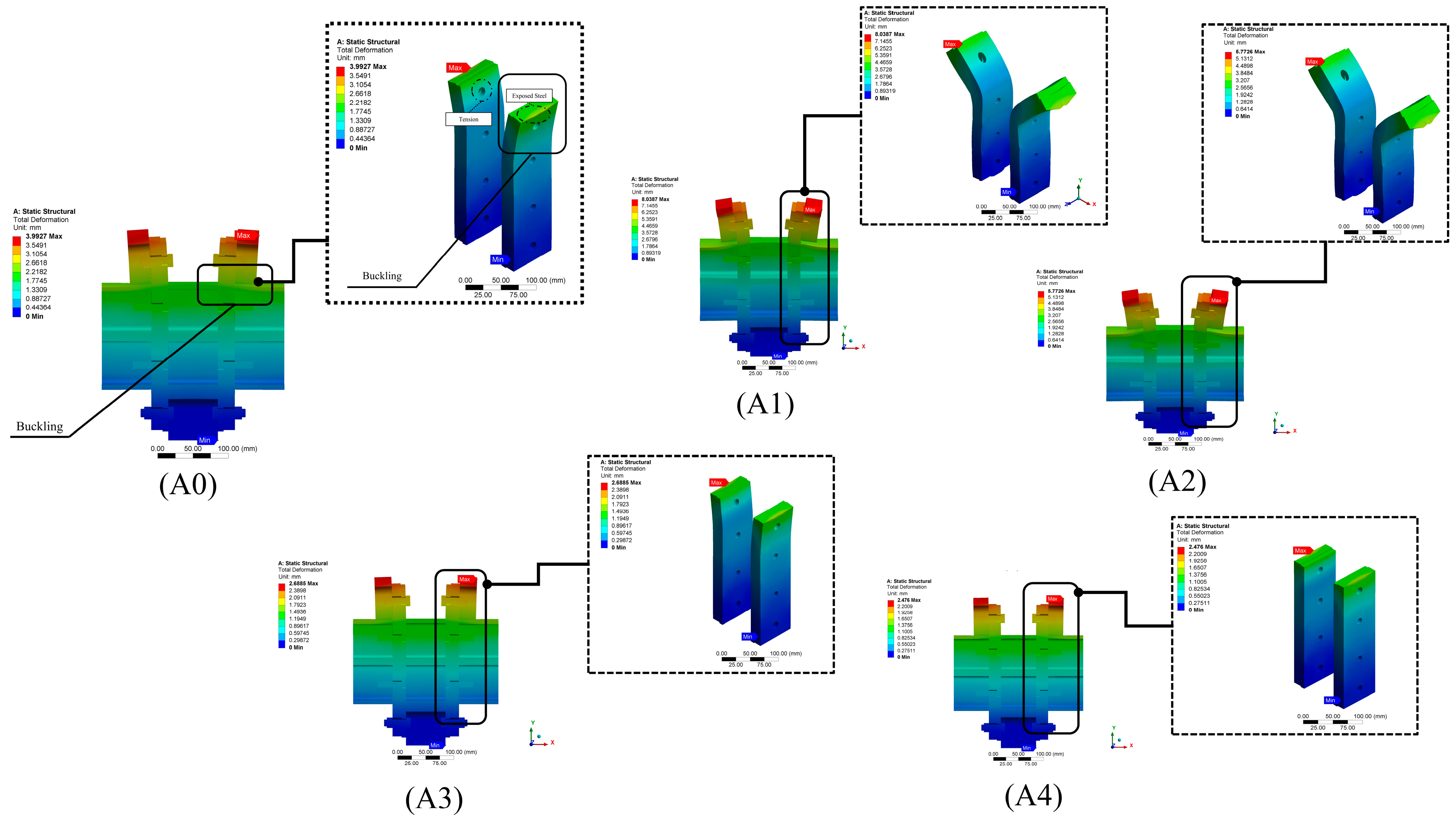
The deformation and buckling in the connection cases of the varying plate thickness and their impact on the connection stability are shown in Figure 10. The controlled model (A0) showed mid-plate buckling, particularly in the 8 mm (SP14) plate, top and bottom regain, tension at the upper bolt holes, and steel exposure near the upper bearing, indicating structural vulnerabilities. Halving the thickness to 4 mm, as in case (A1), exacerbates buckling and tension increase, reflecting the reduced capacity of thinner plates to maintain structural integrity under standard loading conditions. However, it is crucial to acknowledge the uncertainties that might arise when these models are subjected to different loading scenarios, such as seismic or combined axial, lateral, shear, and torsional. A moderate improvement is seen in case (A2), reducing buckling relative to (A1), but it still suffers from notable tension and buckling, indicating improvement requirements. A marked enhancement in the connection resistance is observed in case (A3), where 10 mm plates minimise deformation with a reduction in buckling and tension. The most substantial resistance to buckling is achieved in case (A4), where the thickest plates exhibit the best minor deformation, minimal buckling, tension, and reduced steel exposure.
For closer observation of the plate (SP14) and its bolt deformation across the case studies, Figure 11 shows each case’s failure modes. In the controlled model (A0), buckling presents at the critical stress point (top, bottom, and corner of the plate) alongside tension across the late near to midsection and exposed steel around the bolt holes. Case (A1) presents the severe plate failure scenario with significant steel exposed at both the bottom of the head and the top of the bolt nut. Case (A2) shows a partial recovery from (A1), with plate buckling reduction; however, the plate exhibits considerable tension and exposed steel with tension and rotation alongside the bolt body. The failure modes improved in case (A3); buckling, tension, wear, and exposed steel are significantly diminished in the plate, suggesting a more resilient connection that can better handle the stress applied to the bolts. Case (A4) starts the optimal structural behaviour with minimal buckling, negligible wear, reduced tension, very little exposed steel, and a minor bolt deformation, indicating the most robust connection among all cases. Therefore, it was concluded that the increased plate thickness correlates with enhanced interlocking (IMCs) stability.

3.2. Stability and Stiffness Behaviour

Stiffness measurements investigated the stability and stiffness of the connection configurations across the case studies (A1 to A4) compared to the control model (A0), as illustrated in Figure 12. The investigation reveals that the control model (A0) stiffness consistently maintained zero values, indicating no additional stiffness contribution. Notably, case (A4) stiffness demonstrated the highest stiffness values, reaching a peak of 53.33 kNa/mm at 12.5 kN force, 62.07% higher than the controlled model (A0) stiffness at the same point force and 50.75% lower than case (A3). The lowest stiffness values were recorded in case (A1) with a significant decrease to 2.05 kN/mm at 25 kN point force. This highlights the substantial impact of interlocking (IMCs) plate thickness on the structural integrity of MSBs, with thicker plates markedly enhancing stability and stiffness, potentially offering improved deformation resistance and overall structural robustness.

4. Advanced Predictive Modelling Study

4.1. Polynomial Regression Formula and R-Values

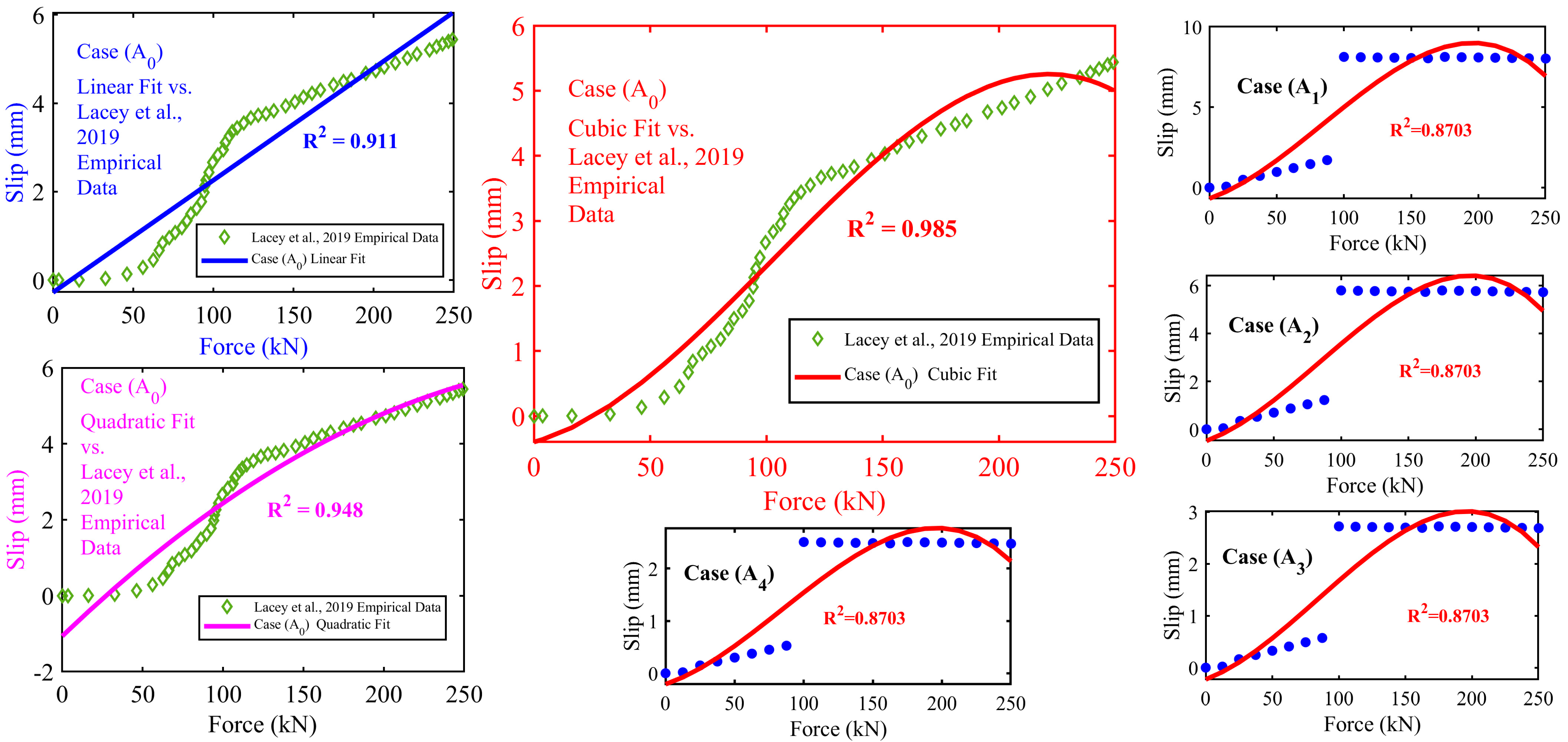
The study developed polynomial regression formulas to predict slip (deformation) across various interlocking (IMCs) plate thickness scenarios. The study utilised empirical data from Lacey et al. [20] to develop a reliable model that predicts slip based on applied force by conducting the following steps using MATLAB R2022b. Multiple polynomial models ranging from 1st degree (linear) to 3rd degree (cubic) were fitted to the data using the ‘Polyfit’ function in MATLAB R2022b. This function calculates the coefficients of polynomials that fit the data in the sense of least squares. Each model’s fit was evaluated using the coefficient of determination (R2), the key indicator of model fit, with a higher value indicating a model that more accurately represents the data. The fits of different polynomial degrees were visually and quantitatively compared, as shown in Figure 13, to create a model that captures the data non-linearities without overfitting. Based on this analysis, a cubic polynomial model was selected. The formula for the controlled model (A0) from the MATLAB R2022b is as follows:
A 0 = 3.46 × F   3 23.25 × F   2 + 67.91 × F + 23.25
where in Equation (1), F is the applied force, and the R2 value is 0.9854, as shown in Figure 13. The coefficients of the additional study models (A1 through A4) were determined, likely through the previous statistic fitting process of the model (A0). The formulas for the polynomial regression from MATLAB R2022b for models (A1 through A4) are the following:
A 1 = - 1.81 × 10 - 6 × F   3 + 4.60 × 10 - 4 × F   2 + 2.90 × 10 - 2 × F - 0.68
A 2 = - 1.29 × 10 - 6 × F   3 + 3.28 × 10 - 4 × F   2 + 2.07 × 10 - 2 × F - 0.48
A 3 = - 6.07 × 10 - 7 × F   3 + 1.53 × 10 - 4 × F   2 + 9.47 × 10 - 3 × F - 0.22
A 4 = - 5.59 × 10 - 7 × F 3 + 1.41 × 10 - 4 × F 2 + 8.94 × 10 - 3 × F - 0.20
The consistent use of cubic polynomial equations across these models was chosen for their ability to capture the complex, accurate, non-linear relationship between applied force and the resultant slip deformation in IMCs. For models A1 through A4, the R2 value is consolidated at 0.8703, as shown in Figure 13.

4.2. Polynomial Regression Model for Slip Prediction

The development and application of a polynomial regression model was designed to predict slip phenomena (∆) in response to a range of applied forces (0 to 250 kN). This model (refer to Appendix B) is central to understanding the intricate non-linear relationships between the forces applied to interlocking mechanisms and the observed slip responses. It is represented mathematically as below:
Slip   ( ) = a n · F   n + a n - 1 · F   n - 1 + + a 1 · F + a 0
Equation (6) captures the essence of the slip prediction model, where (∆) denotes the slip, (F) represents the applied force, and (an) through (a0) are the coefficients that define the curve’s shape based on the degree (n) of the polynomial. These coefficients are critical as they embody the model’s sensitivity to changes in force, enabling the prediction slope with varying degrees of applied forces. The development and implementation of this model were carried out in MALATAB R2022b. This included generating a comprehensive set of force values within the specified range and applying the polynomial coefficients to predict slip outcomes. The process began by defining a vector encompassing 1000 evenly spaced force values between 0 and 250 kN to cover a broad spectrum of potential scenarios. Specific polynomial coefficients were established based on predefined equations for each model variant (A0 through A4). These coefficients are instrumental in delineating the model’s predictive accuracy and were selected to mimic closely the empirical data observed in slip phenomena. Using MALATAB R2022b’s ‘polyval’ function, the polynomial equations were evaluated for each force value, facilitating the slip prediction across the range of applied forces. This pivotal step transforms theoretical constructs into practical, predictive insights that accurately reflect the slip behaviour under various force conditions.

4.3. Validation of Polynomial Regression Model

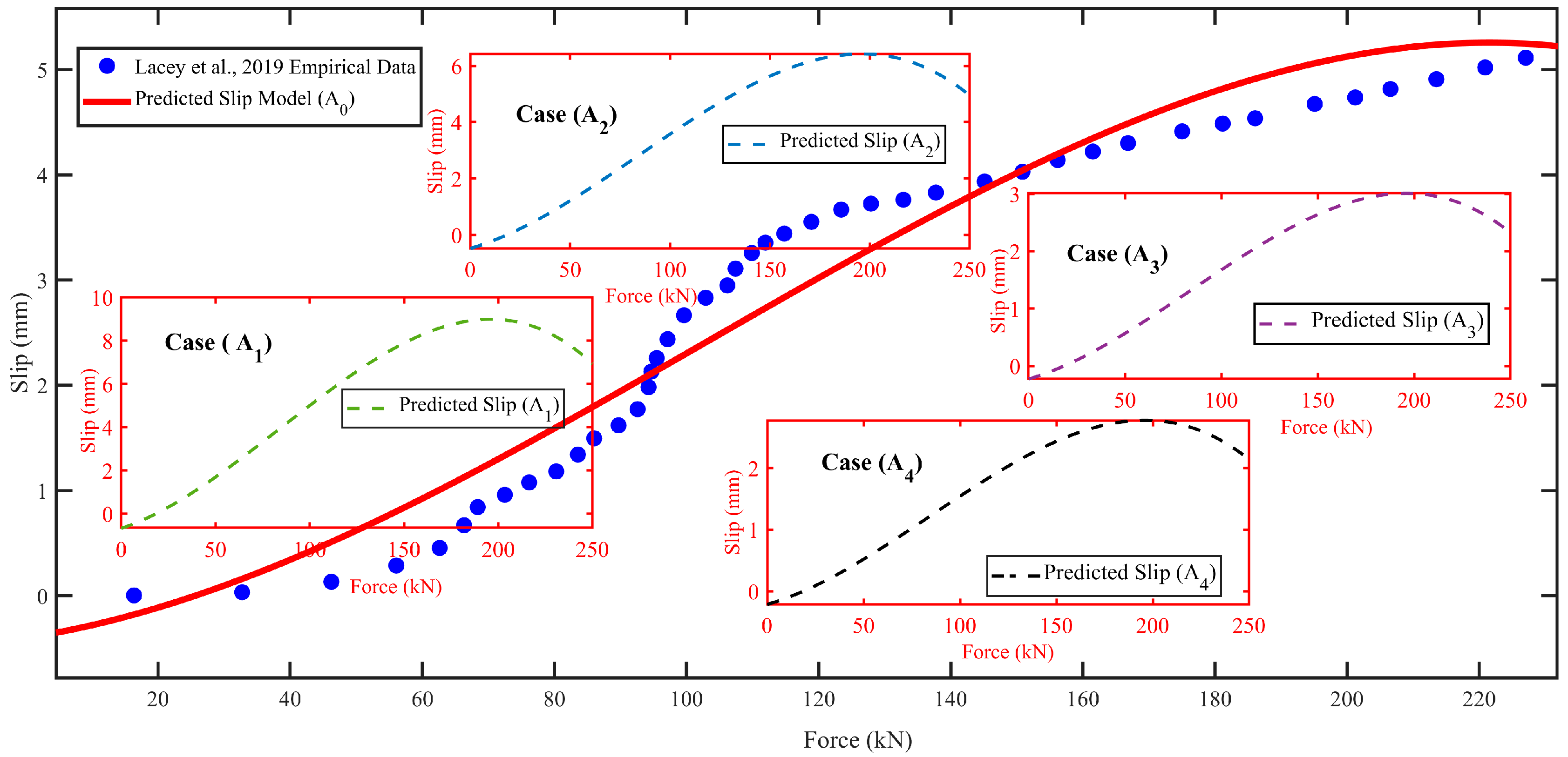
The polynomial regression model, specifically the control model (A0), was validated by comparing its predictions against empirical data from Lacey et al. [20] experiments, as depicted in Figure 14. This comparison evaluated the model’s precision in predicting slip due to varying applied forces, employing MALATAB R2022b for the analytical process. The evaluation revealed a range of accuracy in the model’s predictions. On one end, some predictions showcased exceptional accuracy, with errors as low as 0.11%. Conversely, the model’s predictions diverged significantly from the experimental data at higher slip values, with errors reaching up to 24.16%. This variability highlights the model’s fluctuating accuracy across different force levels.
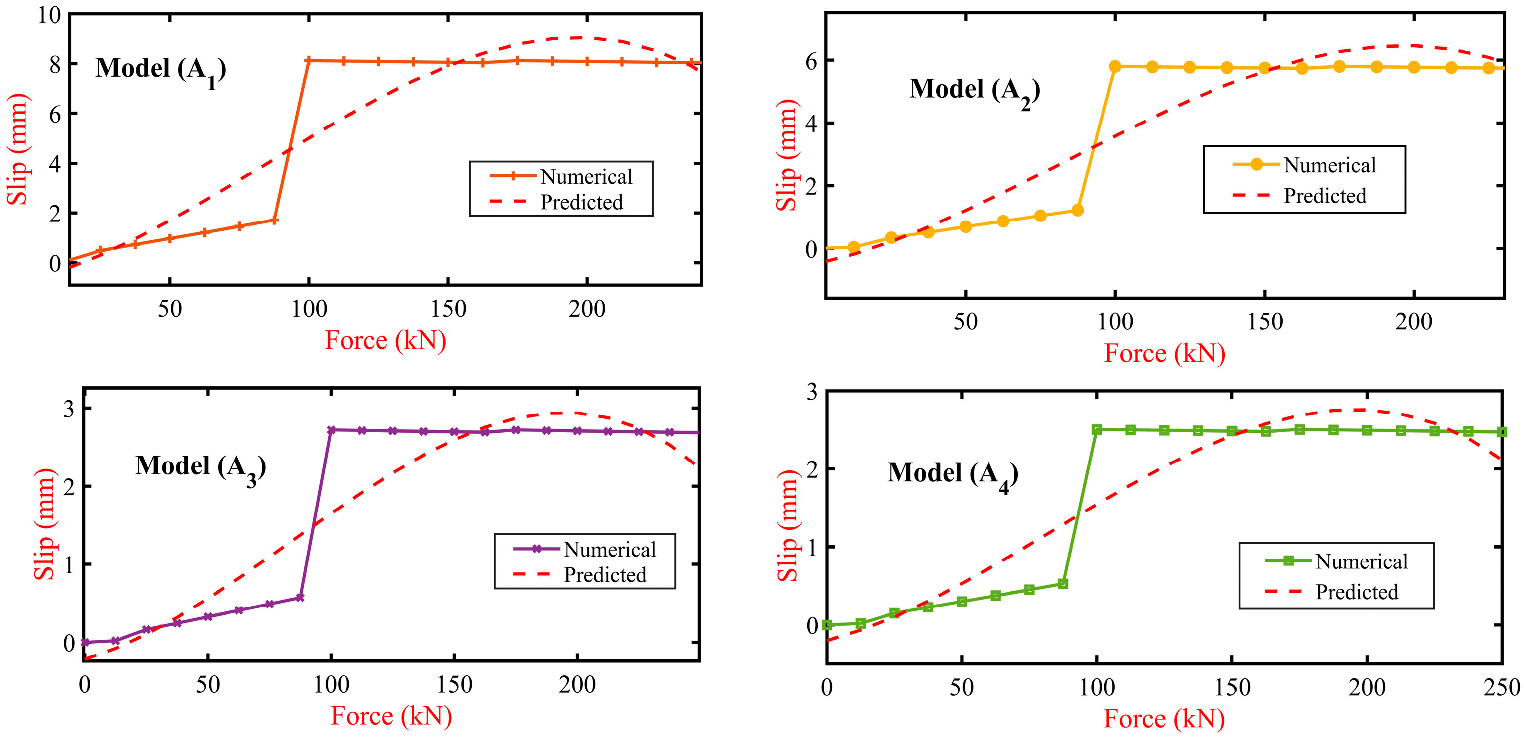
A comprehensive analysis was conducted to quantify the overall performance of the model. The total absolute difference between the model’s predictions and the empirical slip values was approximately 16.30 mm, calculated across all data points, excluding zero slip scenarios, for greater precision. This resulted in an average error rate of approximately 10.80%, indicating a generally commendable level of accuracy in the model’s slip predictions. Further comparisons involved the model’s performance against FE models (A1) through (A4), as detailed in Figure 15. These comparisons revealed varying degrees of accuracy, with the model (A1) exhibiting an average error of about 59.50%, indicating a significant deviation from actual slip values. Models (A2) and (A3) showed slightly better but still considerable error rates of 59.10% and 57.90%, respectively, while model (A4) emerged as the most accurate, with an error rate of approximately 57%. These results underscore the challenges in slip prediction and highlight the potential for refinement in the polynomial regression model’s application.

4.4. Random Forest Regression Model Analysis

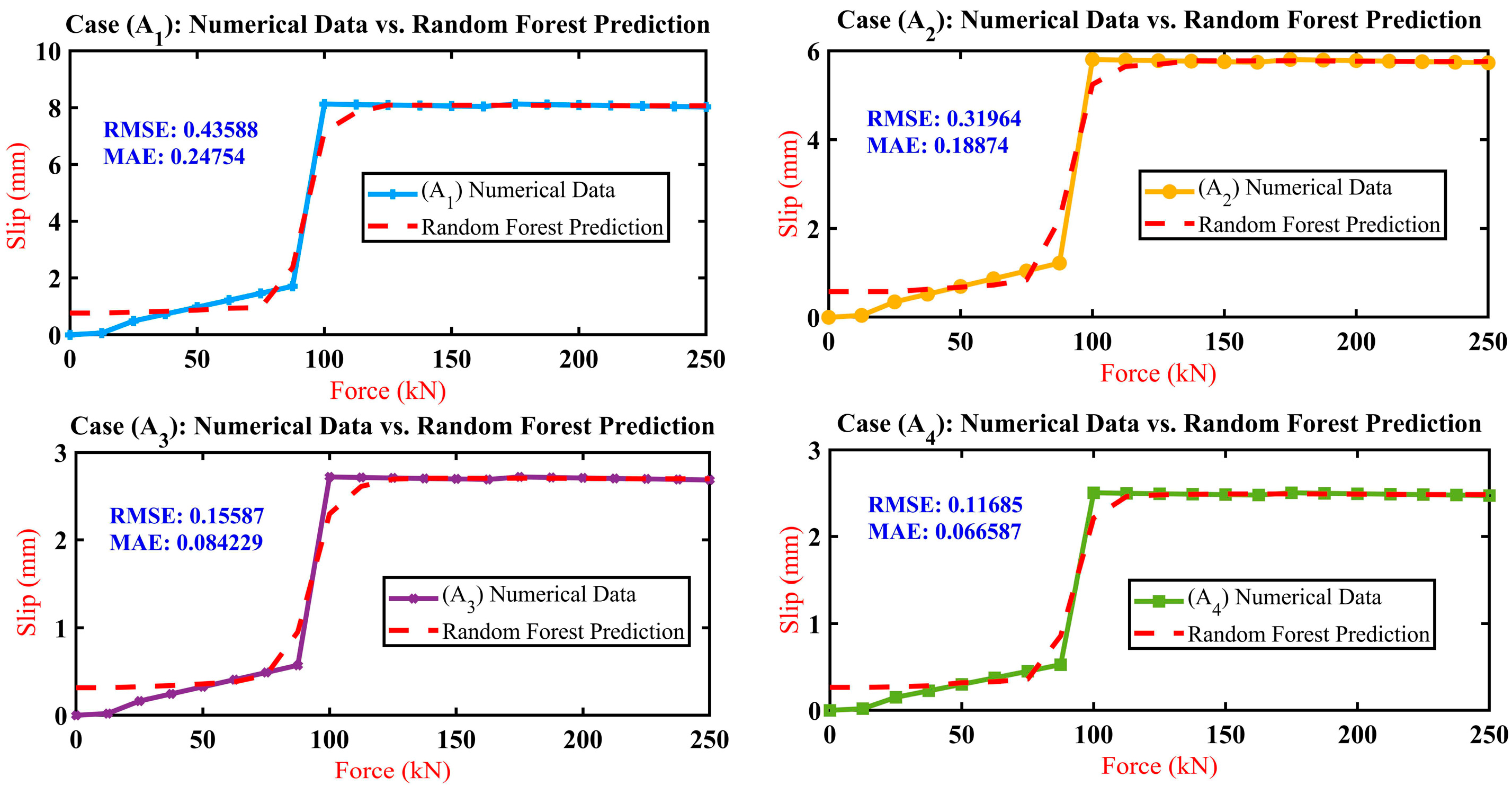
The previous validation approach affirms the model’s efficiency in predicting slip across the range of forces and highlights potential avenues for further refinement. This study delves into deploying a machine-learning model (refer to Appendix C) using the MATLAB R2022b ‘TreeBagger’ function to enhance slip prediction accuracy across various forces. The ‘TreeBagger’ tool employs a random forest regression approach, an ensemble learning method that constructs multiple decision trees during the training phase. This method is renowned for its robustness and flexibility in modelling complex, non-linear relationships without a predefined model structure. Utilising this approach, the study iterated over four sets of slip data (A1 to A4), each employing the applied force as the predictor variable and the corresponding slip values as the response variable. The model was trained for each dataset and subsequently used to predict slip values, plotted against actual data for a visual comparison. Two key metrics were employed to quantify the model’s predictive performance: Mean Absolute Error (MAE) and Root Mean Square Error (RMSE). MAE calculates the average absolute differences between the predicted and actual values, offering a measure resistant to outliers. Conversely, RMSE provides the square root of the average squared differences between predicted and actual values, offering insight into the overall magnitude of the prediction error. A comparative analysis of the model’s performance across the datasets (A1 to A4) revealed that case (A4) exhibited the most favourable outcomes in terms of both RMSE and MAE. This indicates that (A4) had the lowest average error magnitude and demonstrated the highest resilience against outliers. Following (A4), the models’ performance in terms of accuracy improved progressively from (A3) to (A2) and lastly to (A1), as detailed in the results shown in Figure 16. The analysis highlighted a notable overestimation in initial slip predictions for lower forces (0 to 75 kN). However, the model’s predictions for higher forces (above 87.5 kN) closely matched the empirical slip values. For instance, at a force level of 100 kN, the maximum deviation observed was approximately 7%, with the numerical slip at 8.1253 mm and the random forest prediction at 7.193 mm for case (A1). In contrast, for cases (A2) and (A3), the predicted slip values were lower by approximately 11.70% compared to the empirical values at the same force level. In contrast, case (A4) exhibited a slight discrepancy of about 14.80%. In conclusion, the random forest regression analysis, powered by ‘TreeBagger’, underscores the effectiveness of the random forest model in predicting slip across varying forces. This approach highlights the model’s strengths and its potential areas for improvement. The observed trend, starting with an overestimation at lower forces and achieving higher accuracy at greater forces, signals a promising direction towards refining the accuracy of interlocking mechanism models.

5. Advanced Predictive Modelling Study

This study delves into the impact of plate thickness variations on the stiffness characteristics (ranging from stiffness A0 to stiffness A4) of interlocking (IMCs) in MSBs. The core of our analysis involved utilising MATLAB R2022b to conduct a detailed sensitivity analysis, focusing specifically on how changes in applied force influence the stiffness attributes. This involved assessing the rate of stiffness changes to applied force, highlighting the relationship between force fluctuations and stiffness response. The sensitivity analysis using MATLAB R2022b involved (1) checking for errors and anomalies and (2) comparing the sensitivity results with alternative methods (linear regression analysis and anomaly detection).

5.1. Stiffness Sensitivity Analysis

This study delves into the intricacies of how variations in plate thickness influence the stiffness attributes (stiffness A0 to stiffness A4) within interlocking (IMCs) for MSBs. Employing MATLAB R2022b for comprehensive sensitivity analysis, this segment evaluated the derivatives of stiffness in relation to applied force across different attributes, delineating their sensitivity to force alterations through calculated rate changes and visual comparisons with the numerical stiffness metrics. The analytical process unfolds in the following manner: (1) dataset definition, (2) rate of change calculation (derivative), and (3) results visualisation, where the rates of change are plotted alongside the numerical stiffness, as shown in Figure 17.
The insights from this analysis are systematically compiled and presented in Table 4, which encapsulates the average sensitivity across the stiffness attributes. Furthermore, Table 4 expands to mapping the sensitivity variability and underscoring the stiffness attributes’ differential responsiveness to applied forces. The data reveal a gradation in average sensitivity and stiffness across the attributes. Notably, the controlled model (A0) showed an average sensitivity and average stiffness of 2.3441, indicating a moderate responsiveness to force changes. In contrast, case (A1) exhibits the lowest average sensitivity and stiffness (1.1653), suggesting a less pronounced structural response to force variations; case (A2) shows an average sensitivity and stiffness (1.6392) positioned between model (A0) and case (A1), highlighting a balanced approach to stiffness and adaptability. This could imply a strategic design consideration to optimise rigidity and responsiveness to applied forces. The analysis takes a significant turn with the Stiffness case (A3) and case (A4), where a marked increase in average sensitivity and stiffness is observed. (A3), with an average stiffness of 3.4987, alongside case (A4) leading stiffness of 3.7992, underscores a heightened structural response to force applications. This heightened sensitivity and stiffness might reflect a design optimised for environments demanding high durability and adaptability to varying loads, potentially offering enhanced performance in dynamic or unpredictable conditions.

5.2. Errors and Anomalies

How to quantitatively assess the sensitivity of models (A0 through A4) stiffnesses to changes in applied loads and detect and highlight the anomalies that might indicate data inconsistencies, measurements errors or other noteworthy deviations from expected patterns is presented. Anomalies detected at the initial force indices across all attributes highlight the necessity to refine the analysis techniques. Advanced filtering, expressly the Moving Average [68] and SavitzkyGolay filters [69], was incorporated to address these issues. Those methods are proviral in reducing noise and enhancing the signal quality of the stiffness data, which is critical for the accuracy of the predictive models.
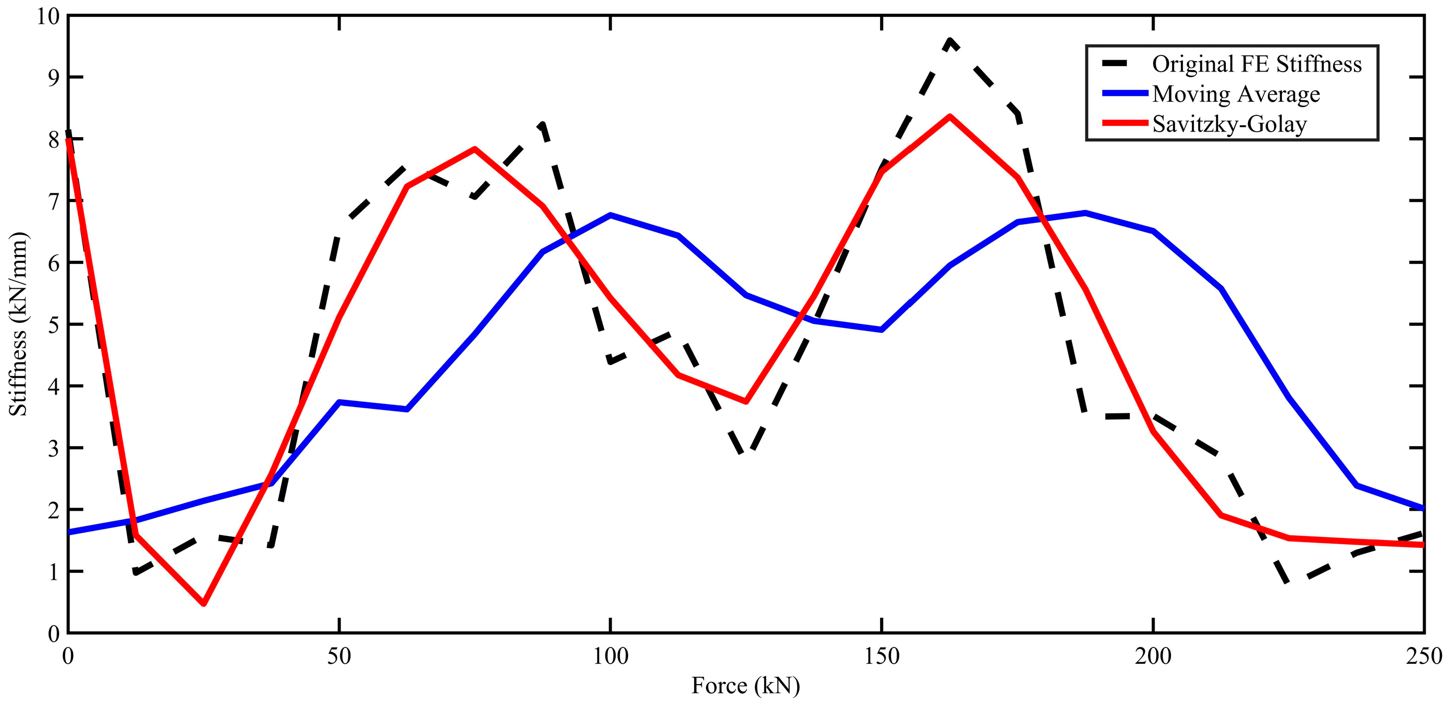
Figure 18 presents the variances between the ‘Original FE stiffness’ measurements and those adjusted by ‘Moving Average’ and ‘SavitzkyGolay’ filtering techniques across the force range. The ‘Original’ data exhibit considerable fluctuation, ranging from lows of 0.75 to highs of 9.39, which obscure actual material behaviour under the force’s applications. While smoothing data, the ‘Moving Average’ approach consistently underestimates stiffness at higher force levels. There were discrepancies as stark as a reduction to 1.204 from an original 6.0198 at 0 kN, suggesting an average dampening effect of 79% compared to ‘Original’. Conversely, the ‘SavitzkyGolay’ filter more closely aligns with the ‘Original’ data, retaining essential features such as peaks and troughs, with deviations being less pronounced, notably preserving higher stiffness values at both lower (6.1128 vs 6.0198 at 0 kN) and higher force applications (9.2539 vs. 9.39 at 250 kN), reflecting an average preservation rate of 98.5% compared to ‘Original’. This comparative analysis underscores the ‘SavitzkyGolay’ method’s superior capability in maintaining data integrity while reducing noise, making it a more reliable approach for interpreting stiffness behaviour under varying forces.

5.3. Stiffness Linear Regression Analysis

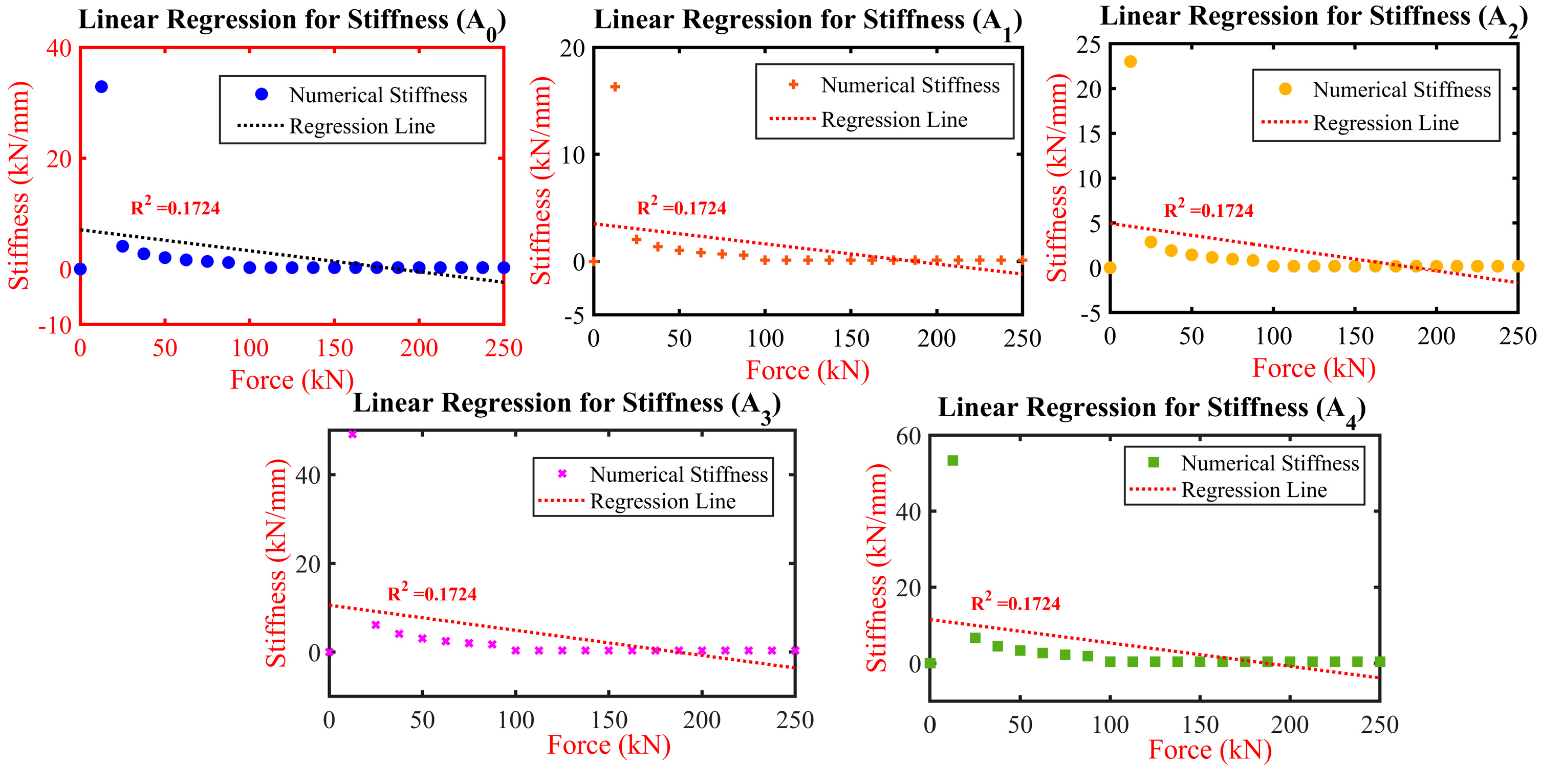
Since the previous study did not investigate the stiffness behaviour of the connection, alternative data analysis and statistics models are utilised to compare the numerical stiffness obtained using ANSYS 2023R2 with the statistical model’s data using the MATLAB R2022b algorithms approach. A linear regression analysis approach was utilised to model the relationship between force and stiffness across various attributes (stiffness A0 to stiffness A4), aimed at understanding how stiffness matrices respond to changes in applied force. The analysis commenced with defining the dataset, consisting of the force value range from 0 to 250 kN at regular intervals and corresponding stiffness measurements for the five attributes (stiffness A0 through stiffness A4); linear regression was then applied to each attribute to model the stiffness as a function of force, and for each stiffness attribute, the analysis process included (1) preparation of data points, associating for each force with its corresponding stiffness measurement, (2) implementation of linear regression, where the force was the independent variable and stiffness measurements acted as the dependent variable, (3) visualisation of the dataset alongside the regression line, highlighting the linear relationship between force and stiffness for each attribute, and (4) calculation of the R-squared value for each regression.
Figure 19 shows the linear regression analysis for stiffness attributes case (A0 through A4) plotted against the applied force. The analysis reveals indication of a negative slope across all the attributes; in case (A0), the intercept is at 7.082 kN/mm, and the stiffness decreases with increasing force, shown by a slope of −0.0379, while in case (A1), started at an intercept of 4.5187 kN/mm, with a gentler decline in stiffness as the force increases, indicated by a slope of −0.0188; in contrast, case (A3) gained at a higher intercept of 10.572 kN/mm, has a more pronounced decrease in stiffness for increased force, as the slope is −0.0565. Finally, case (A4) has a higher intercept at 11.48 kN/mm and the steepest negative slope of −0.0614, indicating the most considerable decrease in stiffness with force among the attributes. The R-squared value for all the attributes is the same (0.1724), indicating that the force explains a small portion of the variability in stiffness and that other factors might also significantly influence stiffness, such as material properties, geometry, load distribution, ageing wear, strain load, defect, etc.

5.4. Anomaly Detection Analysis

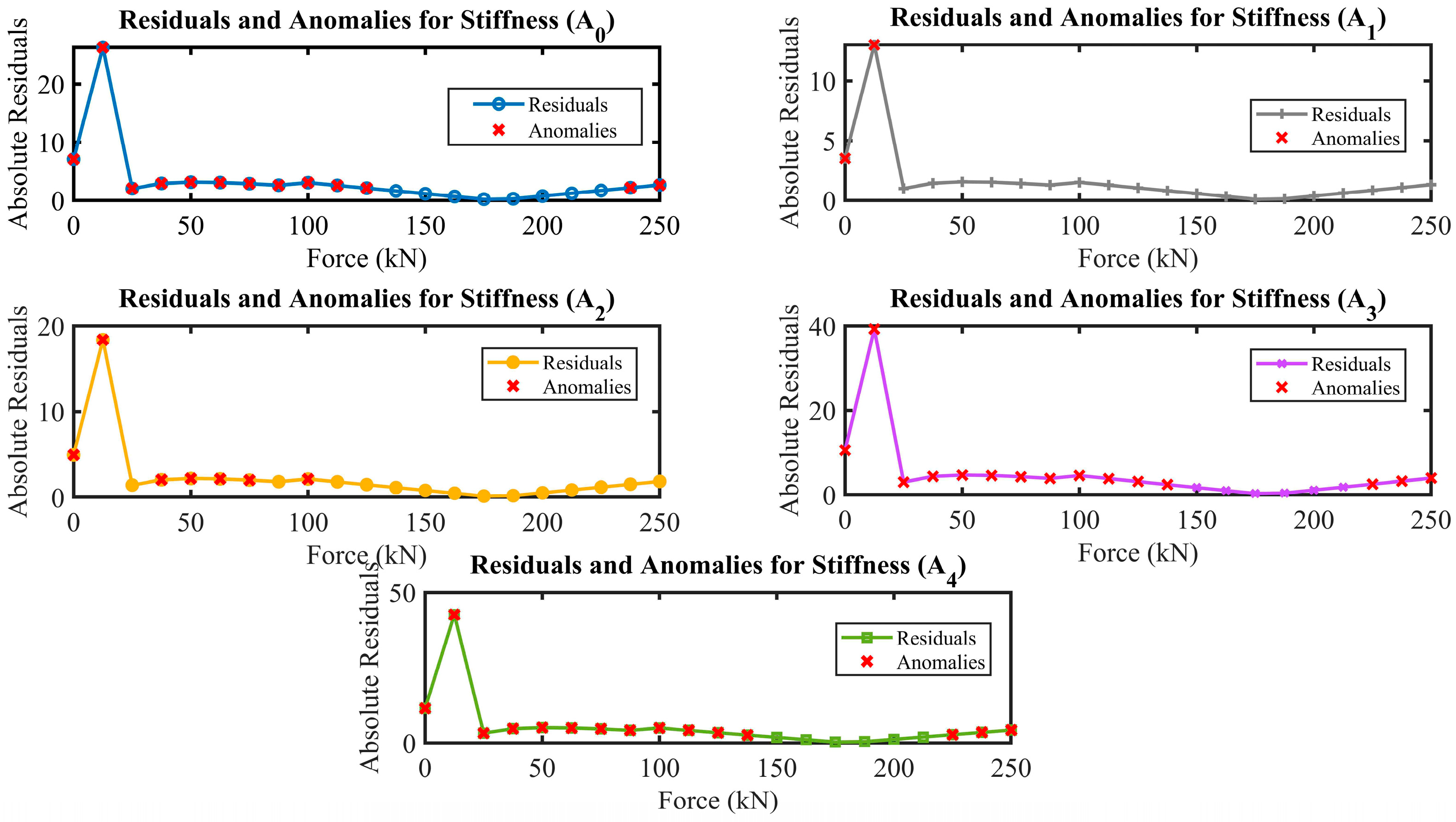
In the context of the study investigation, the anomaly detection approach focused on identifying anomalies through the analysis of residuals derived from linear regression models. This approach is pivotal for elucidating deviations from anticipated linear behaviour across a quintet of stiffness attributes (Stiffness A0 to Stiffness A4) against the applied force range. Employing linear regression, residuals were calculated for each attribute by deducing the difference between the observed values and those predicted by the model. Subsequently, points were identified as anomalies when their absolute residuals surpassed a pre-established threshold. This procedure was instrumental in unveiling a distinct distribution of anomalies across the dataset. As shown in Figure 20, stiffness in the controlled model (A0) presented an extensive array of anomalies, spanning virtually over the entire range of applied forces. This suggests a fundamental non-linearity in the material’s response. In contrast, case (A1) displayed anomalies only at the onset of force application, hinting at potential setup or calibration issues. Case (A2) showed anomalies at scattered force levels, indicating possible specific points of interest in the material’s behaviour under load. Meanwhile, case (A3) and case(A4) exhibited a similar pattern to (A0), with anomalies detected across a broad spectrum of forces, underscoring a need for a deeper investigation into the structural or material properties influencing these observations. In conclusion, analysing residual and anomalies across stiffness attributes provides valuable insights into the expected and potential behaviour of the connection under investigation.

5.5. Interlocking (IMCs) Plate Optimisation

Optimising plate thickness for interlocking IMCs in MSBs is pivotal, necessitating a harmonious blend of material property examination and cost-efficiency evaluation. Leveraging MATLAB R2022b, this study navigated through plate thicknesses ranging from 4 mm to 12 mm to identify the optimal balance between structural integrity and cost-effectiveness, as in Section 2.4. Iteratively, the investigation calculates the yield and tensile strengths against the respective costs for each thickness. The analysis demonstrates a proportional yield increase and tensile strength with plate thickness, affirming a robust correlation with material volume. Conversely, the material cost escalates with increased thickness, which challenges the economic efficiency. The study, therefore, navigates this complexity to ascertain the most efficient plate thickness.
The optimal thickness is 11.03 mm, with a maximum efficiency value of 2.03 × 10⁶ while maintaining structural integrity. This thickness corresponds to a material cost reduction of approximately 8.08% compared to the less efficient thickness option (A4). This decisive finding is graphically depicted in Figure 21.

6. Conclusions

This paper investigated the optimum interlocking (IMCs) plate thickness for MSBs using FE analysis and random forest regression techniques to unveil optimal configurations that balance structural integrity with economic feasibility. The major conclusions and recommendations of the investigations are presented below.
(i)
A plate thickness of 11.03 mm is optimal, yielding significant material cost reductions of approximately 8.08% and enhancing deformation resistance by up to 50.75%, ensuring economic efficiency without comparing structural integrity.
(ii)
Sensitivity analysis underscores that thicker plates (A4) exhibit heightened structural responsiveness and stiffness, significantly improving stability and force distribution by approximately 62.07% more than the controlled model (A0).
(iii)
Implementing advanced anomaly detection techniques markedly improved the predictive accuracy of the predictive models, preserving data integrity at an impressive rate of 98.5%, reducing noise, and improving signal quality compared to original measurements.
(iv)
The ‘TreeBagger’ random forest regression model significantly improved the prediction accuracy of slip values by up to 7% at higher force levels, demonstrating the model’s capability to handle complex relationships effectively.
(v)
Linear regression analysis provided a deep understanding of how stiffness responds to force changes, noting a potential increase in stiffness by up to 50.75% with thicker plates, which fortifies the connection’s stability.
(vi)
Examination of slip phenomena across varying plate thicknesses revealed that the thickest plate (A4) offers superior deformation resistance, reducing slip by approximately 38% compared to the controlled model (A0).
(vii)
The integration of Finite Element analysis with random forest regression has strategically optimised plate thickness, balancing structural robustness with cost efficiency and setting a foundation for future advancements in modular building technologies.
This study was confined to evaluating only four interlocking plate sizes without considering environmental factors such as temperature variations, corrosion, and long-term wear and tear that significantly affect the structural integrity of connections. Furthermore, it does not address the dynamic loading conditions essential for a thorough structural analysis. Future research will focus on assessing the impact of environmental conditions on the durability and resilience of interlocking (IMCs). It will also explore the performance of these connections under dynamic loading, including seismic simulations and variations in live loads, to deepen our understanding of their structural behaviour. More sophisticated predictive models should also be developed that accurately simulate the complex interactions between plate thickness, material properties, and loading conditions. Additionally, exploring alternative materials and innovative connection designs will aim to optimise structural efficiency and sustainability in MSBs, enhancing the design, safety, and versatility of interlocking IMCs and supporting their wider adoption in the construction industry.

Author Contributions

Conceptualization, K.E. and A.A.M.; methodology, K.E. and M.E.; software, K.E., M.E. and M.R.A.; validation, M.E., A.A.M. and M.R.A.; formal analysis, K.E. and A.A.M.; investigation, K.E., M.E. and M.R.A.; resources, K.E. and A.A.M.; data curation, K.E. and M.E.; writing—original draft preparation, K.E. and M.E.; writing—review and editing, A.A.M. and M.R.A.; visualization, K.E. and M.E.; supervision, A.A.M. and M.R.A.; project administration, A.A.M., K.E. and M.E.; funding acquisition, A.A.M. and K.E. All authors have read and agreed to the published version of the manuscript.

Funding

This work was financially supported by the Centre for Research and Instrumentation Management (CRIM), Universiti Kebangsaan Malaysia (UKM) [FRGS/1/2021/TK0/UKM/02/26].

Data Availability Statement

Dataset available on request from the authors.

Conflicts of Interest

The authors declare no conflicts of interest.

Appendix A

>> %% Material Efficiency Optimisation Script
% This script calculates the optimal thickness of a material to maximise
% an efficiency metric defined as the sum of normalised yield and tensile
% strengths divided by the cost. It is designed to be adaptable to different
% materials and scenarios.
%% Step 1: Initialize Parameters
% Define the material properties for the specific material under study.
minYieldStress = 360e6; % Minimum yield stress in Pascals (Pa), for G350 steel
minTensileStrength = 450e6; % Minimum tensile strength in Pascals (Pa), for G350 steel
% Constants and Variables
L = 2; % Span length in meters, adjust as necessary (not used in this script)
c = 100; % Cost per mm thickness of the material
% Define the range of thicknesses to evaluate (in mm)
thicknessRange = linspace(4, 12, 100); % Thickness range from 4mm to 12mm, adjust as necessary
%% Step 2: Pre-allocate Arrays for Storing Computed Values
yieldStrengthValues = zeros(size(thicknessRange));
tensileStrengthValues = zeros(size(thicknessRange));
costValues = zeros(size(thicknessRange));
efficiencyValues = zeros(size(thicknessRange));
%% Step 3: Compute Properties Across Thickness Range
% Loop over each thickness to calculate strength properties and efficiency
for i = 1:length(thicknessRange)
t = thicknessRange(i) / 1000; % Convert thickness from mm to meters
yieldStrengthValues(i) = minYieldStress * (t / 0.004); % Normalize yield strength based on min thickness
tensileStrengthValues(i) = minTensileStrength * (t / 0.004); % Normalize tensile strength similarly
costValues(i) = c * thicknessRange(i); % Calculate cost based on thickness
efficiencyValues(i) = (yieldStrengthValues(i) + tensileStrengthValues(i)) / ...
costValues(i); % Calculate efficiency using ellipsis for line continuation
end
%% Step 4: Identify Optimal Thickness
[optimalValue, optimalIndex] = max(efficiencyValues); % Find maximum efficiency and its index
optimalThickness = thicknessRange(optimalIndex); % Determine optimal thickness
%% Step 5: Output Results
fprintf('Optimal Thickness for Maximum Efficiency: %.2f mm\n', optimalThickness);
fprintf('Maximum Efficiency Value: %.2f\n', optimalValue);
%% Step 6: Visualization of Results
% Plotting yield strength, tensile strength, and efficiency versus thickness
figure;
subplot(3, 1, 1);
plot(thicknessRange, yieldStrengthValues, 'b-', 'LineWidth', 2);
title('Yield Strength vs. Thickness');
xlabel('Thickness (mm)');
ylabel('Yield Strength (Pa)');
subplot(3, 1, 2);
plot(thicknessRange, tensileStrengthValues, 'r-', 'LineWidth', 2);
title('Tensile Strength vs. Thickness');
xlabel('Thickness (mm)');
ylabel('Tensile Strength (Pa)');
subplot(3, 1, 3);
plot(thicknessRange, efficiencyValues, 'g-', 'LineWidth', 2);
title('Efficiency vs. Thickness');
xlabel('Thickness (mm)');
ylabel('Efficiency (Strength/Cost)');
sgtitle('Material Efficiency Optimization Analysis');
%% Step 7: Save Results (Optional)
% Optionally, save results to a .mat file or other formats for further analysis
save('OptimizationResults.mat', 'thicknessRange', 'yieldStrengthValues', 'tensileStrengthValues', 'costValues', 'efficiencyValues', 'optimalThickness', 'optimalValue');

Appendix B

>> % MATLAB Script for Predictive Analysis of Slip Based on Applied Forces
% Utilizes polynomial regression models to predict slip in response to applied forces,
according to specified equations (Eq. 1 to Eq. 5).
% Step 1: Define the force range for prediction
% Generating a vector of 1000 evenly spaced force values between 0 and 250 kN.
force_values = linspace(0, 250, 1000); % linspace(start, end, number of points)
% Step 2: Define polynomial coefficients for each model based on provided equations
% Polynomial Regression Formula for Slip (A0) as per Eq. 1
coeffs_A0 = [3.46, -23.25, 67.91, 23.25]; % Coefficients for Model A0 with R^2 = 0.9854
% Polynomial Regression Formulas for Slips (A1 to A4) as per Eqs. 2 to 5
coeffs_A1 = [−1.81×10⁻⁶, 4.60×10⁻⁴, 2.90×10⁻², −0.68]; % Model A1 with R^2 = 0.8703
coeffs_A2 = [−1.29×10⁻⁶, 3.28×10⁻⁴, 2.07×10⁻², −0.48]; % Model A2 with R^2 = 0.8703
coeffs_A3 = [−6.07×10⁻⁷, 1.53×10⁻⁴, 9.47×10⁻³, −0.22]; % Model A3 with R^2 = 0.8703
coeffs_A4 = [−5.59×10⁻⁷, 1.41×10⁻⁴, 8.94×10⁻³, −0.20]; % Model A4 with R^2 = 0.8703
% Step 3: Calculation of predicted slip using polynomial evaluation
% This step evaluates the polynomials for each force value, using the polyval function.
predicted_slip_A0 = polyval(coeffs_A0, force_values); % Prediction for Model A0 (Eq. 1)
predicted_slip_A1 = polyval(coeffs_A1, force_values); % Prediction for Model A1 (Eq. 2)
predicted_slip_A2 = polyval(coeffs_A2, force_values); % Prediction for Model A2 (Eq. 3)
predicted_slip_A3 = polyval(coeffs_A3, force_values); % Prediction for Model A3 (Eq. 4)
predicted_slip_A4 = polyval(coeffs_A4, force_values); % Prediction for Model A4 (Eq. 5)
% Step 4: Aggregation of predicted slips into a matrix for comparative analysis
predicted_slips = [predicted_slip_A0; predicted_slip_A1; predicted_slip_A2;
predicted_slip_A3; predicted_slip_A4]';
% Step 5: Tabulation of results for analysis and visualization
% Creates a table with force values and predicted slips for each model.
results_table = array2table([force_values', predicted_slips], ...
'VariableNames', {'Force_kN', 'PredictedSlip_A0', 'PredictedSlip_A1',
'PredictedSlip_A2', 'PredictedSlip_A3', 'PredictedSlip_A4'});
% Display the results table to the MATLAB command window for review and analysis.

Appendix C

>> function trainAndPlotRandomForestModels(Force, SlipData)
% Train and plot random forest models for given force and slip data sets.
% Force: A vector of force values.
% SlipData: A cell array where each cell contains a vector of slip values for a
different model (A1 to A4).
nTrees = 100; % Number of trees in the random forest
for i = 1:length(SlipData)
Y = SlipData{i}';
% Train the random forest model
model = TreeBagger(nTrees, Force', Y, 'Method', 'regression');
% Predict slip values using the trained model
Y_pred = predict(model, Force');
% Plot actual vs. predicted slip values
figure;
plot(Force, Y, 'bo', 'MarkerFaceColor', 'b'); hold on;
plot(Force, Y_pred, 'r-', 'LineWidth', 2);
hold off;
xlabel('Force (kN)');
ylabel(sprintf('Slip A%d', i));
title(sprintf('Model A%d: Numerical Data vs. Random Forest Prediction', i));
legend('Numerical Data', 'Random Forest Prediction', 'Location', 'NorthWest');
grid on;
end
end
% Example usage:
Force = [0, 12.5, 25, 37.5, 50, 62.5, 75, 87.5, 100, 112.5, 125, 137.5, 150, 162.5, 175,
187.5, 200, 212.5, 225, 237.5, 250];
Slip_A1 = [0, 0.061275458, 0.486733848, 0.730097368, 0.973440468, 1.216919704,
1.461488028, 1.709255548, 8.12527716, 8.10553744, 8.08920112, 8.07218412, 8.0558478,
8.0388308, 8.12527716, 8.10553744, 8.08920112, 8.07218412, 8.0558478, 8.0388308,
8.0218138];
% Repeat for Slip_A2, Slip_A3, Slip_A4 as needed
SlipData = {Slip_A1}; % Add Slip_A2, Slip_A3, Slip_A4 as available
trainAndPlotRandomForestModels(Force, SlipData);

References

  1. Luo, F.J.; Bai, Y.; Hou, J.; Huang, Y. Progressive Collapse Analysis and Structural Robustness of Steel-Framed Modular Buildings. Eng. Fail. Anal. 2019, 104, 643–656. [Google Scholar] [CrossRef]
  2. Swami, G.; Thai, T.; Thai, H.-T. Modelling Methods for Robustness Analysis of Composite Steel- Concrete Modular Buildings. In Proceedings of the 3rd International Conference on Structural Engineering Research (iCSER2022), Sydney, Australia, 27–30 November 2022. [Google Scholar]
  3. Farajian, M.; Sharafi, P.; Bigdeli, A.; Eslamnia, H.; Rahnamayiezekavat, P. Experimental Study on the Natural Dynamic Characteristics of Steel-Framed Modular Structures. Buildings 2022, 12, 587. [Google Scholar] [CrossRef]
  4. Palmiotta, A.; Garbellini, S.; Audisio, L.; Sulla, R.; D’Amato, M.; Gigliotti, R. Seismic Behaviour of Steel Modular Buildings: Numerical Analysis and Comparisons between Different Design Solutions. Procedia Struct. Integr. 2022, 44, 1156–1163. [Google Scholar] [CrossRef]
  5. Liu, X.; He, X.; Zhang, A.; Tian, C.; Zhang, X.; Tan, Y. Design and Specification Compilation of a Modular-Prefabricated High-Rise Steel Frame Structure with Diagonal Braces Part II: Elastic–Plastic Time-History Analysis and Joint Design. Struct. Des. Tall Spec. Build. 2018, 27, e1414. [Google Scholar] [CrossRef]
  6. Alembagheri, M.; Sharafi, P.; Hajirezaei, R.; Tao, Z. Anti-Collapse Resistance Mechanisms in Corner-Supported Modular Steel Buildings. J. Constr. Steel Res. 2020, 170, 106083. [Google Scholar] [CrossRef]
  7. Chen, Z.; Zhong, X.; Liu, Y.; Liu, J. Analytical and Design Method for the Global Stability of Modular Steel Buildings. Int. J. Steel Struct. 2021, 21, 1741–1758. [Google Scholar] [CrossRef]
  8. Yang, C.; Xu, B.; Xia, J.; Chang, H.; Chen, X.; Ma, R. Mechanical Behaviors of Inter-Module Connections and Assembled Joints in Modular Steel Buildings: A Comprehensive Review. Buildings 2023, 13, 1727. [Google Scholar] [CrossRef]
  9. Poudel, B.; Lee, S.; Choi, J.O. Steel Module-to-Concrete Core Connection Methods in High Rise Buildings: A Critical Review. In Proceedings of the 9th International Conference on Construction Engineering and Project Management, Las Vegas, NV, USA, 20–23 June 2022. [Google Scholar]
  10. Lacey, A.W.; Chen, W.; Hao, H.; Bi, K. Review of Bolted Inter-Module Connections in Modular Steel Buildings. J. Build. Eng. 2019, 23, 207–219. [Google Scholar] [CrossRef]
  11. Swami, G.; Thai, H.T.; Liu, X. Structural Robustness of Composite Modular Buildings: The Roles of CFST Columns and Inter-Module Connections. Structures 2023, 48, 1491–1504. [Google Scholar] [CrossRef]
  12. Chen, Z.; Khan, K.; Khan, A.; Javed, K.; Liu, J. Exploration of the Multidirectional Stability and Response of Prefabricated Volumetric Modular Steel Structures. J. Constr. Steel Res. 2021, 184, 106826. [Google Scholar] [CrossRef]
  13. Chen, Z.; Wang, J.; Liu, J.; Khan, K. Seismic Behavior and Moment Transfer Capacity of an Innovative Self-Locking Inter-Module Connection for Modular Steel Building. Eng. Struct. 2021, 245, 112978. [Google Scholar] [CrossRef]
  14. Srisangeerthanan, S.; Hashemi, M.J.; Rajeev, P.; Gad, E.; Fernando, S. Review of Performance Requirements for Inter-Module Connections in Multi-Story Modular Buildings. J. Build. Eng. 2020, 28, 101087. [Google Scholar] [CrossRef]
  15. Thai, H.T.; Ngo, T.; Uy, B. A Review on Modular Construction for High-Rise Buildings. Structures 2020, 28, 1265–1290. [Google Scholar] [CrossRef]
  16. Lacey, A.; Chen, W.; Hao, H.; Bi, K. Shear Stiffness of Bolted Inter-Module Connections. In Proceedings of the 11th International Conference of the IFHS on Extreme Engineering, Singapore, 28–30 August 2019. [Google Scholar]
  17. He, X.-H.-C.; Chan, T.-M.; Chung, K.-F. Effect of Inter-Module Connections on Progressive Collapse Behaviour of MiC Structures. J. Constr. Steel Res. 2021, 185, 106823. [Google Scholar] [CrossRef]
  18. Shi, F.W.; Ding, Y.; Zong, L.; Meng, X.; Chen, Y. Axial Mechanical Behavior of Innovative Inter-Module Connection for Modular Steel Constructions. J. Build. Eng. 2023, 65, 105765. [Google Scholar] [CrossRef]
  19. Lacey, A.W.; Chen, W.; Hao, H.; Bi, K. New Interlocking Inter-Module Connection for Modular Steel Buildings: Simplified Structural Behaviours. Eng. Struct. 2021, 227, 111409. [Google Scholar] [CrossRef]
  20. Lacey, A.W.; Chen, W.; Hao, H.; Bi, K. New Interlocking Inter-Module Connection for Modular Steel Buildings: Experimental and Numerical Studies. Eng. Struct. 2019, 198, 109465. [Google Scholar] [CrossRef]
  21. Chen, Z.; Wang, J.; Liu, J.; Cong, Z. Tensile and Shear Performance of Rotary Inter-Module Connection for Modular Steel Buildings. J. Constr. Steel Res. 2020, 175, 106367. [Google Scholar] [CrossRef]
  22. Lacey, A.W.; Chen, W.; Hao, H.; Bi, K. Simplified Structural Behaviours of Post-Tensioned Inter-Module Connection for Modular Buildings. J. Constr. Steel Res. 2020, 175, 106347. [Google Scholar] [CrossRef]
  23. Lacey, A.W.; Chen, W.; Hao, H.; Bi, K.; Tallowin, F.J. Shear Behaviour of Post-Tensioned Inter-Module Connection for Modular Steel Buildings. J. Constr. Steel Res. 2019, 162, 105707. [Google Scholar] [CrossRef]
  24. Chen, Z.; Liu, Y.; Zhong, X.; Liu, J. Rotational Stiffness of Inter-Module Connection in Mid-Rise Modular Steel Buildings. Eng. Struct. 2019, 196, 109273. [Google Scholar] [CrossRef]
  25. Chua, Y.S.; Pang, S.D.; Liew, J.Y.R.; Dai, Z. Robustness of Inter-Module Connections and Steel Modular Buildings under Column Loss Scenarios. J. Build. Eng. 2022, 47, 103888. [Google Scholar] [CrossRef]
  26. Peng, J.; Hou, C.; Shen, L. Numerical Simulation of Weld Fracture Using Cohesive Interface for Novel Inter-Module Connections. J. Constr. Steel Res. 2020, 174, 106302. [Google Scholar] [CrossRef]
  27. Lacey, A.W.; Chen, W.; Hao, H.; Bi, K. Lateral Behaviour of Modular Steel Building with Simplified Models of New Inter-Module Connections. Eng. Struct. 2021, 236, 112103. [Google Scholar] [CrossRef]
  28. Shi, F.W.; Ding, Y.; Zong, L.; Chen, Y.; Wu, Y. Shear Behaviour of Vertical Inter-Module Connection with Bolts and Shear Keys for MSCs. Structures 2023, 47, 260–281. [Google Scholar] [CrossRef]
  29. Peng, J.; Hou, C.; Shen, L. Lateral Resistance of Multi-Story Modular Buildings Using Tenon-Connected Inter-Module Connections. J. Constr. Steel Res. 2021, 177, 106453. [Google Scholar] [CrossRef]
  30. Zhao, F.; Yu, Y.; Lin, S.; Ding, F. Evaluation of the Working Mechanisms and Simplified Models of Endplate-Type Inter-Module Connections. Structures 2021, 32, 562–577. [Google Scholar] [CrossRef]
  31. Lim, R.Z.C.; Looi, D.T.W.; Chen, M.T.; Tsang, H.H.; Wilson, J.L. A Component-Based Macro-Mechanical Model for Inter-Module Connections in Steel Volumetric Buildings. J. Constr. Steel Res. 2023, 207, 107954. [Google Scholar] [CrossRef]
  32. Alembagheri, M.; Sharafi, P.; Hajirezaei, R.; Samali, B. Collapse Capacity of Modular Steel Buildings Subject to Module Loss Scenarios: The Role of Inter-Module Connections. Eng. Struct. 2020, 210, 110373. [Google Scholar] [CrossRef]
  33. Corfar, D.A.; Tsavdaridis, K.D. A Hybrid Inter-Module Connection for Steel Modular Building Systems with SMA and High-Damping Rubber Components. Eng. Struct. 2023, 289, 116281. [Google Scholar] [CrossRef]
  34. Lacey, A.W.; Chen, W.; Hao, H. Experimental Methods for Inter-Module Joints in Modular Building Structures—A State-of-the-Art Review. J. Build. Eng. 2022, 46, 103792. [Google Scholar] [CrossRef]
  35. Farajian, M.; Sharafi, P.; Kildashti, K. The Influence of Inter-Module Connections on the Effective Length of Columns in Multi-Story Modular Steel Frames. J. Constr. Steel Res. 2021, 177, 106450. [Google Scholar] [CrossRef]
  36. Dai, Z.; Pang, S.D.; Liew, J.R. Axial Load Resistance of Grouted Sleeve Connection for Modular Construction. Thin-Walled Struct. 2020, 154, 106883. [Google Scholar] [CrossRef]
  37. He, Z.; Zhang, T.; Li, T. Static Bearing Capacity Investigation of Grouted Square Hollow Section Sleeve Connection. Adv. Struct. Eng. 2022, 25, 3–13. [Google Scholar] [CrossRef]
  38. Dai, Z.; Cheong, T.Y.C.; Pang, S.D.; Liew, J.Y.R. Experimental Study of Grouted Sleeve Connections under Bending for Steel Modular Buildings. Eng. Struct. 2021, 243, 112614. [Google Scholar] [CrossRef]
  39. Faculty, E. Review of Interconnection in Modular Structures. In Proceedings of the PACE 2021-Ataturk University, Engineering Faculty, Department of Civil Engineering, Erzurum, Turkey, 20–23 June 2021; pp. 1–8. [Google Scholar]
  40. Lee, Y.H.; Tan, C.S.; Mohammad, S.; Md Tahir, M.; Shek, P.N. Review on Cold-Formed Steel Connections. Sci. World J. 2014, 2014, 951216. [Google Scholar] [CrossRef] [PubMed]
  41. Nadeem, G.; Safiee, N.A.; Bakar, N.A.; Karim, I.A.; Nasir, N.A.M. Connection Design in Modular Steel Construction: A Review. Structures 2021, 33, 3239–3256. [Google Scholar] [CrossRef]
  42. Pang, S.D.; Liew, J.Y.R.L.; Dai, Z.; Wang, Y. Prefabricated Prefinished Volumetric Construction Joining Tech-Niques Review. In Proceedings of the Modular and Offsite Construction (MOC) Summit Proceedings, Edmonton, AB, Canada, 29 September–1 October 2016; pp. 249–256. [Google Scholar] [CrossRef]
  43. Rajanayagam, H.; Poologanathan, K.; Gatheeshgar, P.; Varelis, G.E.; Sherlock, P.; Nagaratnam, B.; Hackney, P. A-State-Of-The-Art Review on Modular Building Connections. Structures 2021, 34, 1903–1922. [Google Scholar] [CrossRef]
  44. Li, Z.; Tsavdaridis, K.D.; Gardner, L. A Review of Optimised Additively Manufactured Steel Connections for Modular Building Systems. In Industrializing Additive Manufacturing; Springer International Publishing: Cham, Switzerland, 2021; pp. 357–373. [Google Scholar]
  45. Srisangeerthanan, S.; Hashemi, M.J.; Rajeev, P.; Gad, E.F.; Fernando, S. A Review of Diaphragm Behaviour and Connections for Multi-Story Modular Buildings. In Proceedings of the Australasian Structural Engineering Conference 2018 (ASEC2018), Adelaide, Australia, 25–28 September 2018. [Google Scholar]
  46. Corfar, D.-A.; Tsavdaridis, K.D. A Comprehensive Review and Classification of Inter-Module Connections for Hot-Rolled Steel Modular Building Systems. J. Build. Eng. 2022, 50, 104006. [Google Scholar] [CrossRef]
  47. Chua, Y.S.; Liew, J.Y.R.; Pang, S.D. Modelling of Connections and Lateral Behavior of High-Rise Modular Steel Buildings. J. Constr. Steel Res. 2020, 166, 105901. [Google Scholar] [CrossRef]
  48. Elsayed, M.A.; Mutalib, A.; Elsayed, K. Numerical Study of Structural Performance and Wind Flow Dynamic Behavior for PPVC Steel Modular Construction (MSC) under Various Extreme Wind Loads. Buildings 2022, 12, 1347. [Google Scholar] [CrossRef]
  49. Sharafi, P.; Mortazavi, M.; Samali, B.; Ronagh, H. Interlocking System for Enhancing the Integrity of Multi-Storey Modular Buildings. Autom. Constr. 2018, 85, 263–272. [Google Scholar] [CrossRef]
  50. Chen, Z.; Liu, J.; Yu, Y. Experimental Study on Interior Connections in Modular Steel Buildings. Eng. Struct. 2017, 147, 625–638. [Google Scholar] [CrossRef]
  51. Chen, Z.; Liu, J.; Yu, Y.; Zhou, C.; Yan, R. Experimental Study of an Innovative Modular Steel Building Connection. J. Constr. Steel Res. 2017, 139, 69–82. [Google Scholar] [CrossRef]
  52. Sanches, R.; Mercan, O.; Roberts, B. Experimental Investigations of Vertical Post-Tensioned Connection for Modular Steel Structures. Eng. Struct. 2018, 175, 776–789. [Google Scholar] [CrossRef]
  53. Chen, X.W.; Yuan, H.X.; Real, E.; Du, X.X.; Schafer, B.W. Experimental Behaviour of Stainless Steel Plate Girders under Combined Bending and Shear. J. Constr. Steel Res. 2020, 166, 105900. [Google Scholar] [CrossRef]
  54. Bazarchi, E.; Davaran, A.; Lamarche, C.P.; Roy, N.; Parent, S. Experimental and Numerical Investigation of a Novel Vertically Unconstrained Steel Inter-Modular Connection. Thin-Walled Struct. 2023, 183, 110364. [Google Scholar] [CrossRef]
  55. Ma, R.; Xia, J.; Chang, H.; Xu, B.; Zhang, L. Experimental and Numerical Investigation of Mechanical Properties on Novel Modular Connections with Superimposed Beams. Eng. Struct. 2021, 232, 111858. [Google Scholar] [CrossRef]
  56. Wu, C.; Zhou, Y.; Liu, J.; Mou, B.; Shi, J. Experimental and Finite Element Analysis of Modular Prefabricated Composite Beam-Column Interior Joints. J. Build. Eng. 2021, 43, 102853. [Google Scholar] [CrossRef]
  57. Nadeem, G.; Safiee, N.A.; Bakar, N.A.; Karim, I.A.; Mohd Nasir, N.A. Experimental and Numerical Study of Self-Locking Adaptable Inter Connection for Modular Steel Structures. J. Build. Eng. 2023, 65, 105723. [Google Scholar] [CrossRef]
  58. Deng, E.F.; Yan, J.B.; Ding, Y.; Zong, L.; Li, Z.X.; Dai, X.M. Analytical and Numerical Studies on Steel Columns with Novel Connections in Modular Construction. Int. J. Steel Struct. 2017, 17, 1613–1626. [Google Scholar] [CrossRef]
  59. Luo, F.J.; Ding, C.; Styles, A.; Bai, Y. End Plate–Stiffener Connection for SHS Column and RHS Beam in Steel-Framed Building Modules. Int. J. Steel Struct. 2019, 19, 1353–1365. [Google Scholar] [CrossRef]
  60. Yu, Y.; Chen, Z. Rigidity of Corrugated Plate Sidewalls and Its Effect on the Modular Structural Design. Eng. Struct. 2018, 175, 191–200. [Google Scholar] [CrossRef]
  61. Deng, E.F.; Zong, L.; Ding, Y.; Dai, X.M.; Lou, N.; Chen, Y. Monotonic and Cyclic Response of Bolted Connections with Welded Cover Plate for Modular Steel Construction. Eng. Struct. 2018, 167, 407–419. [Google Scholar] [CrossRef]
  62. Deng, E.F.; Zong, L.; Ding, Y. Numerical and Analytical Study on Initial Stiffness of Corrugated Steel Plate Shear Walls in Modular Construction. Steel Compos. Struct. 2019, 32, 347–359. [Google Scholar] [CrossRef]
  63. Keipour, N.; Valipour, H.R.; Bradford, M.A. Structural Behaviour of Steel-Timber versus Steel-Concrete Composite Joints with Flush End Plate. Constr. Build. Mater. 2020, 262, 120885. [Google Scholar] [CrossRef]
  64. Elsayed, K.; Mutalib, A.A.; Elsayed, M.; Azmi, M.R. Numerical Study of PPVC Modular Steel Constructions (MSCs) with Selected Connection Strategies under Varied Earthquake Scenarios. Results Eng. 2024, 22, 102076. [Google Scholar] [CrossRef]
  65. Ansys Inc. ANSYS Mechanical 2023; Ansys Inc.: Canonsburg, PA, USA, 2023. [Google Scholar]
  66. The MathWorks Inc. MATLAB, Version: 9.13.0 (R2022b); The MathWorks Inc.: Natick, MA, USA, 2022. Available online: https://www.mathworks.com(accessed on 5 February 2024).
  67. Lacey, A.W.; Chen, W.; Hao, H.; Bi, K. Structural Response of Modular Buildings—An Overview. J. Build. Eng. 2018, 16, 45–56. [Google Scholar] [CrossRef]
  68. Gao, Y.; Mosalam, K.M.; Chen, Y.; Wang, W.; Chen, Y. Auto-Regressive Integrated Moving-Average Machine Learning for Damage Identification of Steel Frames. Appl. Sci. 2021, 11, 6084. [Google Scholar] [CrossRef]
  69. Roy, I.G. An Optimal Savitzky–Golay Derivative Filter with Geophysical Applications: An Example of Self-potential Data. Geophys. Prospect. 2020, 68, 1041–1056. [Google Scholar] [CrossRef]
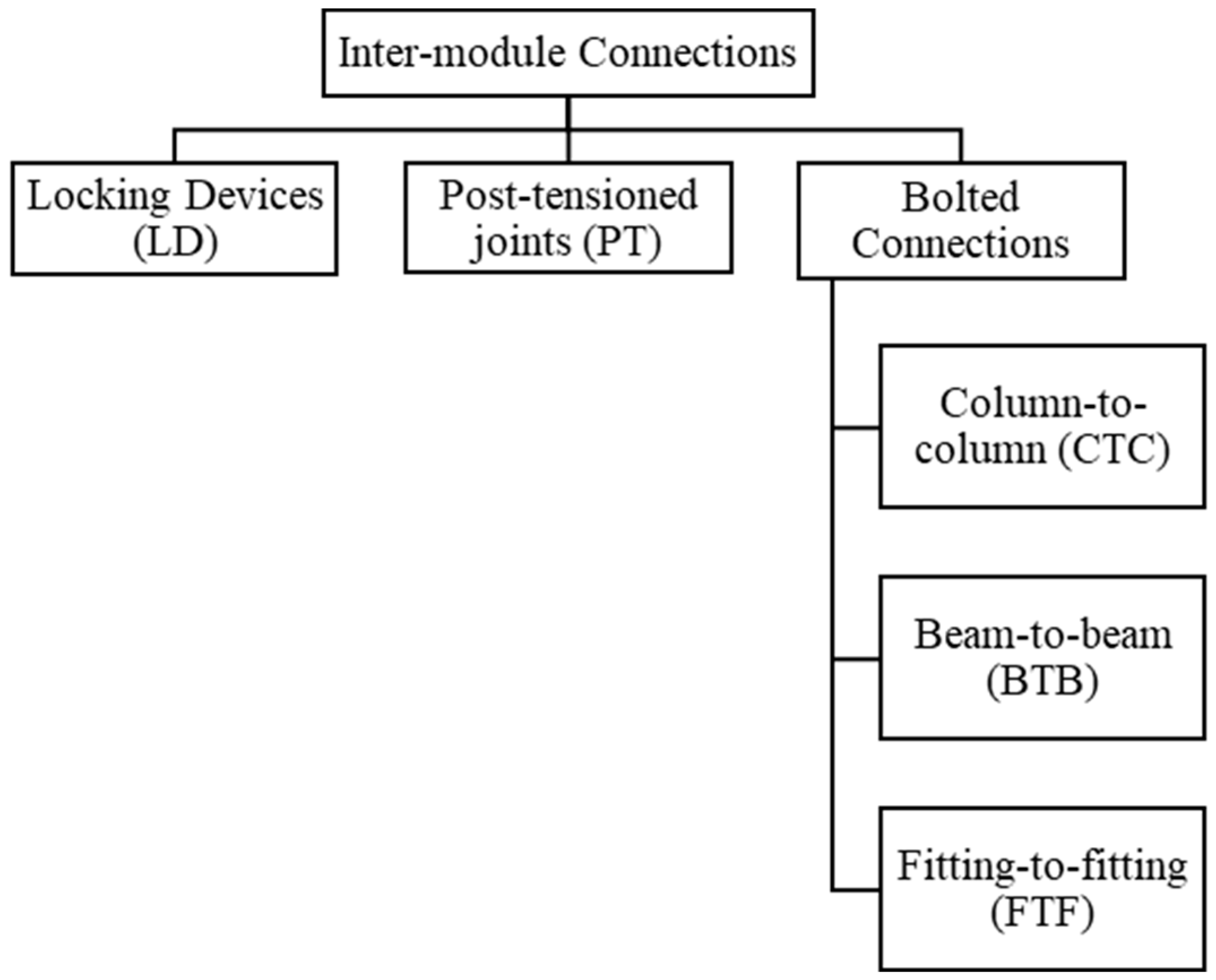
Figure 1. Classification of inter-module connections (IMCs) [46].
Buildings 14 01254 g001
Figure 2. Lacey et al. [20], inter-module connection (CTC).
Buildings 14 01254 g002
Figure 3. Illustration of Lacey et al. [20] specimen (A). Reprinted/adapted with permission from Ref. [20]. Copyright 2019, Elsevier.
Buildings 14 01254 g003
Figure 4. Comparative thickness of plates SP14, SP15, SP16.
Buildings 14 01254 g004
Figure 5. Conceptual view of Lacey et al. [20] experimental setup. Reprinted/adapted with permission from Ref. [20]. Copyright 2019, Elsevier.
Buildings 14 01254 g005
Figure 6. Comparative analysis between force-slip Lacey et al. [20] experimental approach results and FE model mesh size results.
Buildings 14 01254 g006
Figure 7. Loading and boundary conditions in ANSYS 2023 R2.
Buildings 14 01254 g007
Figure 8. FE model (1.0, 2.0, and 4.0 mm) mesh size.
Buildings 14 01254 g008
Figure 9. Comparison of slip behaviour between connection plate thickness cases, including Lacey et al. [20] case (A0).
Buildings 14 01254 g009
Figure 10. Deformation and buckling behaviour for models (A0) to (A4).
Buildings 14 01254 g010
Figure 11. Comparison of (SP14) plate and bolt deformation across models (A0) to (A4).
Buildings 14 01254 g011
Figure 12. Impact of plate thickness Interlocking (IMCs) stiffness behaviour.
Buildings 14 01254 g012
Figure 13. R2 coefficients of polynomial fits for case (A0) against Lacey et al. [20] empirical data and models (A1–A4).
Buildings 14 01254 g013
Figure 14. Comparison of the predicted slip (∆) and Lacey et al. [20] experimental results.
Buildings 14 01254 g014
Figure 15. Comparison between FE models (A1, A2, A3, and A4) slip and the polynomial regression predicted slips.
Buildings 14 01254 g015
Figure 16. Comparison between FE models (A1, A2, A3, and A4) slip and random forest prediction.
Buildings 14 01254 g016
Figure 17. Sensitivity analysis of stiffness attributes in interlocking (IMCs) across applied forces.
Buildings 14 01254 g017
Figure 18. Comparative analysis of ‘Original FE Stiffness’ and filtered data across force range.
Buildings 14 01254 g018
Figure 19. Linear regression analysis of stiffness vs applied force for attributes (A0 to A4).
Buildings 14 01254 g019
Figure 20. Residuals and anomalies in stiffness attributes under varying forces.
Buildings 14 01254 g020
Figure 21. Comparative analysis of Yield Strength, Tensile Strength, and Efficiency across plate thicknesses for IMCs in MSBs.
Buildings 14 01254 g021
Table 1. Cross-section dimensions of Lacey et al. [20] specimen (A) model. Reprinted/adapted with permission from Ref. [20]. Copyright 2019, Elsevier.
DescriptionPartCross-Section Dimensions (mm)Length (mm)Illustration Ref.
Hollow SectionSP1075 × 75 × 650Figure 3
Hollow SectionSP1275 × 75 × 670
Square BarUpper Bearing75 × 75 × 3075
Lower Bearing75 × 75 × 60
Round BarSP11R1250
PlateSP1475 × 875
PlateSP1575 × 875
PlateSP1675 × 8135
Bolt (B)M12,8.8 Grade-24
Table 2. Material properties.
PartGradeMin. Yield Stress (MPa)Min. Tensile Strength (MPa)Min. Elongation (%)
SP10, SP12C350L035043012
Bearings30029044022
SP1130037553034
SP14, SP15, SP16G35036045020
Bolt (B)Class 8.864080012
Table 3. Thickness variation of plates SP14, SP15, SP16.
Plate(A0) Thickness (mm)(A1) Thickness (mm)(A2) Thickness (mm)(A3) Thickness (mm)(A4) Thickness (mm)
SP148461012
SP158461012
SP168461012
Table 4. Range and average rate of change in stiffness.
Stiffness AttributeMin Rate of ChangeMax Rate of ChangeAverage Rate of Change
(A0)−2.30342.63240.00099828
(A1)−1.14121.30560.00049864
(A2)−1.61081.84090.0006981
(A3)−3.43793.9290.00149
(A4)−3.73324.26650.001618
Disclaimer/Publisher’s Note: The statements, opinions and data contained in all publications are solely those of the individual author(s) and contributor(s) and not of MDPI and/or the editor(s). MDPI and/or the editor(s) disclaim responsibility for any injury to people or property resulting from any ideas, methods, instructions or products referred to in the content.