Article

Integrated Interactive Control of Distribution Systems with Multi-Building Microgrids Based on Game Theory

Electric Power Research Institute State Grid Anhui Electric Power Co., Ltd., Hefei 230022, China
*
Author to whom correspondence should be addressed.
Buildings 2024, 14(2), 325; https://doi.org/10.3390/buildings14020325
Submission received: 26 September 2023 / Revised: 14 November 2023 / Accepted: 22 December 2023 / Published: 24 January 2024
(This article belongs to the Special Issue Strategies for Building Energy Efficiency)

Abstract

:
In the transactional processes within a multi-building microgrid system, it is imperative to safeguard stakeholders’ interests and ensure stable, economically efficient operation. Therefore, this paper proposes an integrated interactive control of distribution systems with multi-building microgrids based on game theory. Initially, an interactive framework encompassing superior power grids, distribution network operators, and multi-building microgrids is proposed. This framework establishes a master–slave game model between distribution network operators and multi-building microgrids. Additionally, it introduces the concept of Soft Open Points between building microgrids to enhance system operational safety while also reducing economic costs for distribution network operators. Subsequently, to maintain solution accuracy and optimality, it employs linearization and cone relaxation methods to transform the original model into a mixed-integer second-order cone programming model. Furthermore, it enhances an iterative search method and the price mechanism based on supply and demand ratios. The revised price mechanism serves to boost the participation of building microgrid users in energy regulation, while the iterative search method effectively resolves the equilibrium point of interest among all game participants. Finally, a simulation analysis is conducted on an IEEE-33 test system, and the effectiveness of the proposed strategy is verified by comparing three schemes.

1. Introduction

According to the latest report from the New Strategy Research Institute for Energy Security in 2021, China’s wind power capacity has grown to 330 million kW, while its solar power generation capacity stands at an impressive 310 million kW. Both these figures mark a remarkable increase of over 15% compared to the previous year. This substantial growth can be attributed to the strong guidance provided by national strategies and policies [1]. Looking ahead, it is anticipated that China’s wind energy sector will continue to witness rapid expansion, with an estimated annual growth rate of 80 million kilowatts over the next five years. Consequently, the large-scale integration of renewable energy sources into the power grid has emerged as a dominant trend [2]. Addressing the challenge of promoting local distributed energy (DG) consumption while ensuring the power grid’s reliability, safety, and economic viability is now an urgent imperative.
Building microgrids (BMGs) have emerged as pivotal components within modern power systems owing to their exceptional attributes, including high efficiency, environmental friendliness, adaptability, and self-sufficiency [3]. They not only function as autonomous and self-contained systems but also facilitate information and energy exchange across vast regions through flexible interconnections among multiple building microgrids. This collaborative approach serves to mitigate transmission losses, reduce overall system operating expenses, and elevate system-wide flexibility and reliability.
Research on methods for energy interactions in multi-building microgrid (MBMG) systems can be mainly divided into two categories: those based on direct control and those centered around distributed interactions facilitated by local energy markets. The direct control method [3,4] primarily originates from the perspective of the upper-level power grid or distribution network operator (DNO). In this approach, the upper-level power grid or operator acquires information from building microgrids and exerts centralized control over all manageable components, simplifying system-wide operations. However, this method harbors potential drawbacks, including transaction congestion, elevated maintenance costs, privacy concerns, and limited scalability.
In contrast, the distributed method founded on local energy markets takes into account the interests of all stakeholders. Through decentralized coordination, it harmonizes control decisions within the flexible distribution network, enabling effective management of internally distributed energy resources by building microgrids. This approach facilitates resource sharing and safeguards the interests of autonomous management systems [5]. The existing body of research on distributed methods encompasses various approaches, including those grounded in multi-building microgrid systems [6], game theory [7], auction theory [8], and semi-market regulatory frameworks [9]. However, while the aforementioned research provides valuable insights for the application of distributed methods, certain limitations persist. On the one hand, the literature [6,7] often overlooks the integrated study of both economic aspects related to multi-BMG transactions and the technical intricacies of flexible distribution network operations. This oversight may result in the inability to simultaneously optimize voltage regulation and overall operational economics [10]. On the other hand, the literature [6,11] insufficiently considers load requirement transferability, potentially resulting in discrepancies between theoretical and real-world outcomes, leading to improper regulation of system components. Such oversights not only hinder economic optimization but also pose security risks to the distribution network system.
First, it is crucial to acknowledge that economic and safe operation considerations are often interdependent. The transaction decisions made between the lower-level MBMG and the upper-level DNO can exert a significant influence on the overall performance of the distribution network. Failing to account for the operational state of the power grid may lead to overutilization of power grid assets and result in severe voltage violations. Furthermore, the potential for centralized power consumption can exacerbate the power imbalance among feeders [12], thereby disrupting power flow and substantially increasing system power losses [10]. Hence, this paper introduces an interactive energy regulation optimization model based on the local energy market to simultaneously minimize operational costs and rectify voltage violations.
Simultaneously, it is worth noting that many existing studies [8,13] have employed network reconfiguration to alter the topology of the distribution network (DN) for power flow adjustments. While this approach has achieved the objectives of reducing network losses and mitigating voltage overvoltage fluctuations, its performance can still be enhanced. The limitation lies in the operating frequency constraints of tie switches. Soft Open Points (SOPs) are novel, fully controlled power electronic devices known for their rapid response characteristics [10,14]. SOPs have the capability to precisely and continuously regulate the active and reactive power of connected feeders. In contrast to network reconfiguration, SOPs hold greater significance in power flow regulation [11]. Remarkably, there is an unexplored potential for SOP application in the realm of energy trading. In light of this, this article incorporates SOPs into a multi-building microgrid distribution system grounded in the principles of the local energy market. This integration serves the purpose of actively regulating the voltage within the distribution network, attenuating the impact of energy transactions on the system’s power flow. Consequently, this not only further diminishes network losses but also curtails the operating costs incurred by the DNO.
Furthermore, apart from the challenge of balancing voltage stability and operational economy in MBMG transactions, facilitating residual power trading for building microgrid users engaged in these transactions is of paramount importance. A fundamental driver of electricity trading lies in the establishment of robust electricity pricing structures. Without appropriate pricing mechanisms, it becomes a formidable task to encourage energy sharing coupled with effective demand response (DR) mechanisms. Hence, considering the inherent uncertainty introduced by the integration of electric vehicles, it is notable that the literature [15] has pioneered the development of a multi-building microgrid Bayesian bidding game model to facilitate electricity trading amongst BMGs. In a similar vein, the literature [16] has crafted a model that addresses buyer selection and seller price competition within the context of Peer-to-Peer (P2P) power trading [17,18]. However, this particular model restricts its scope to the operations of a single-building microgrid user. Likewise, the literature [19] delves into electricity trading between multiple building microgrids but confines its focus to real-time electricity prices. Building microgrid users solely devise bidding strategies at the current moment without involvement in the day-ahead market. Correspondingly, the literature [20] primarily concentrates on real-time transaction models between operators and users, employing the Shapley value as the transaction price. Furthermore, the literature [21] formulates a model relying on the Shapley value as the transaction price, which safeguards the internal interests of the system but falls short of ensuring the interests of the entire system. From a different perspective, the literature [22] endeavors to harmonize interests between the distribution network and BMGs but does not account for BMGs as independent entities capable of engaging in electricity trading. To address these gaps, this article takes into consideration the economic interests of various entities within the MBMG system. It enhances the 24 h day-ahead pricing mechanism based on the supply and demand ratio, striking a balance among the interests of diverse entities and fostering the active participation of BMGs in electricity trading.
Given the backdrop described above, this paper undertakes a comprehensive examination of the competition dynamics within the MBMG system transactions. This investigation encompasses a range of influential factors, including photovoltaic output, SOP utilization, On-Load Tap Changer (OLTC) settings, energy storage system (ESS) charging and discharging operations, and internal transactions. To address these complexities, this paper introduces an integrated interactive control method of multi-agent flexible distribution systems (MFDS) based on a master–slave game. The salient features of this paper are reflected in Table 1 by comparing existing studies on energy interaction control. Our main contributions are as follows:
(1)
Building upon P2P transactions, this paper introduces a master–slave game model tailored for 24 h distribution networks and MBMG systems. This innovative model not only prioritizes the maximization of the DNO interests as the leader but also incorporates the price elasticity behaviors of individual BMG users;
(2)
Addressing nonlinear models, this study employs linearization techniques and second-order cone relaxation methods to transform the initial model into a mixed integer second-order cone programming model to ensure both solution accuracy and optimality;
(3)
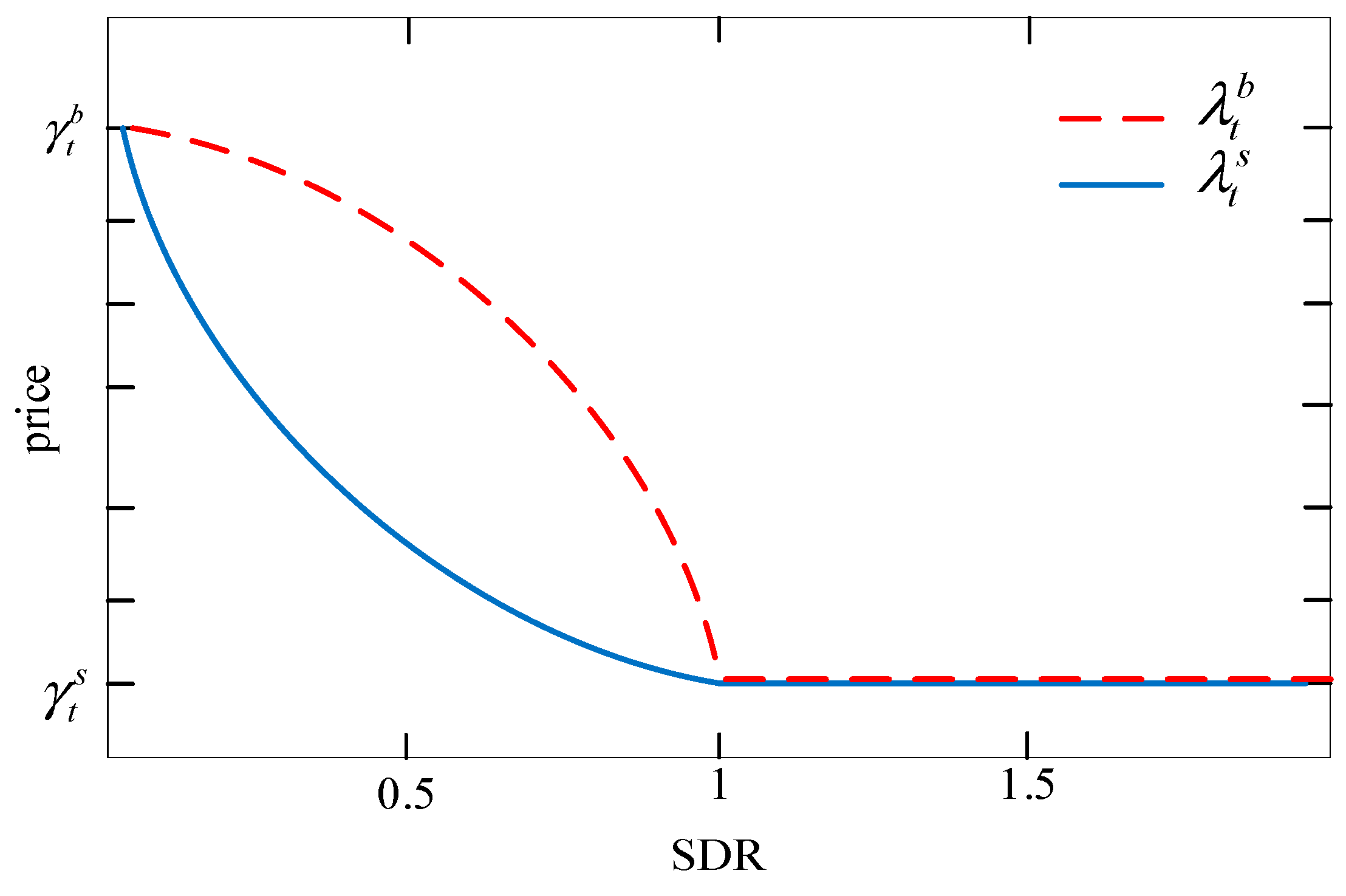
The price mechanism of supply and demand ratio (SDR) has been improved, and the two-way trading between power grids and multi-building microgrid systems has been considered. These enhancements effectively encourage the active engagement of building microgrid users in energy regulation and the localized utilization of distributed energy resources.
Table 1. Comparative features of previous energy interaction control studies.
ReferenceSOP IntegrationVoltage RegulationDemand ResponseBalancing the Interest of MGs and DNO
[3,4]Yes
[5,8,11]YesYes
[10]YesYes
[11,14,15,16,17,18,19]YesYes
Proposed methodYesYesYesYes

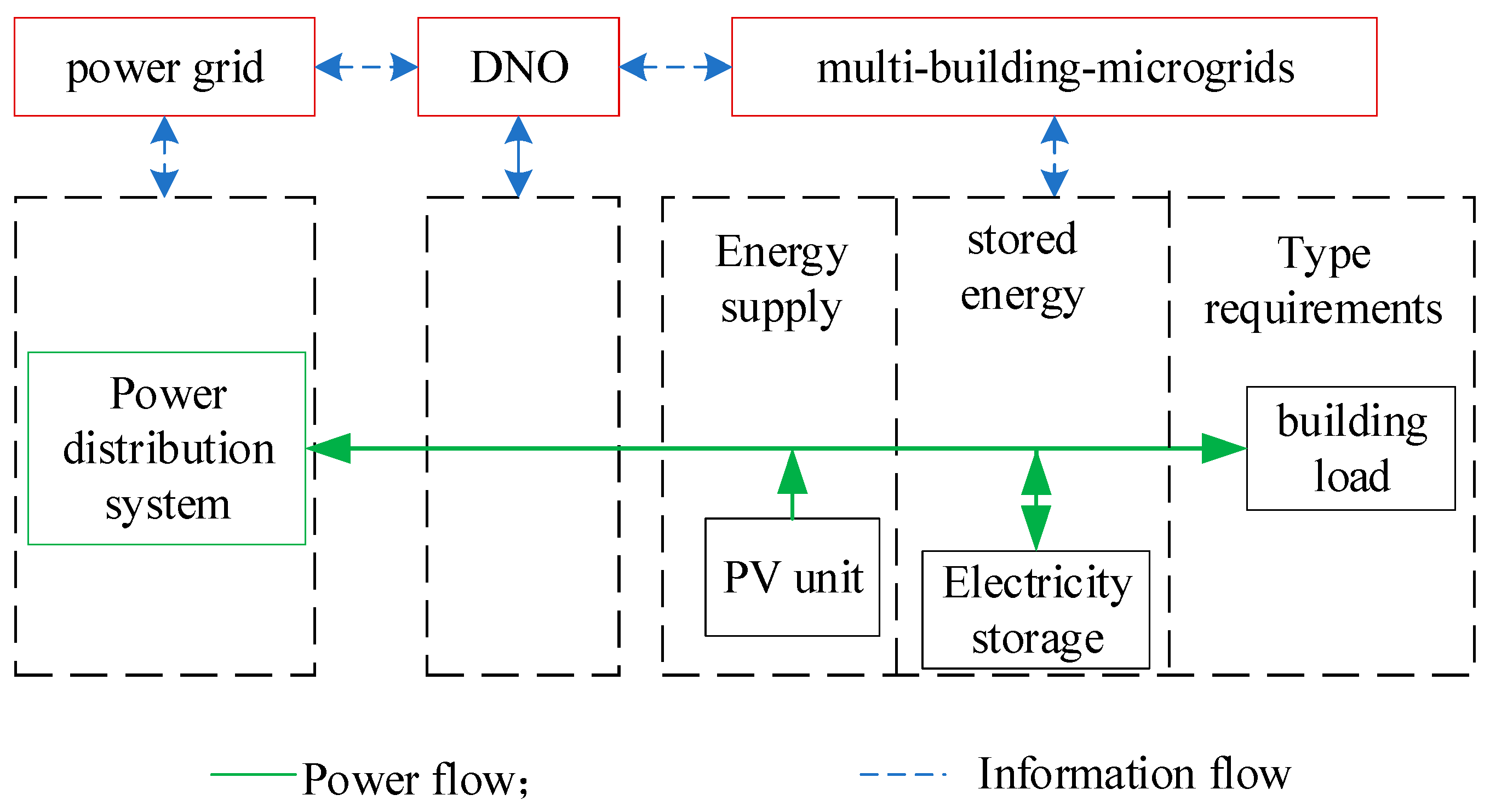
2. MFDS Interactive Framework

2.1. Physical and Market Structure

The MFDS interaction framework constructed in this article is shown in Figure 1. From the physical point of view, it includes three main parts: (1) energy supply, provided by external power distribution systems and BMG photovoltaic units; (2) energy storage, to achieve the storage and release of electric energy; and (3) type requirements (mainly building loads, including general loads and controllable loads). In addition, this article assumes that the electric energy generated in a multi-building microgrid system can not only be consumed but also transmitted to the superior power grid system.
The MFDS interactive energy market consists of three parts: the superior power network, DNO, and MBMG. The high-speed and reliable two-way information interaction among the three parts provides the foundation for timely price and demand information interaction. The superior power grid is the setter of external energy prices.
The DNO is the operator and internal electricity price setter of the DN, controlling SOP and OLTC devices, and is responsible for conducting electricity transactions with the superior power grid and MBMG. The DNO can optimize supply and demand, enhance on-site renewable energy consumption, balance distribution system safety and technical performance with BMG economic performance, and maximize its own benefits through electric energy pricing and management. The MBMG is a follower of internal electricity prices, and each BMG is composed of photovoltaic (PV), energy storage systems (ESSs), general loads, and controllable loads. In addition, SOPs are installed between BMGs for more accurate and fast power regulation. Each BMG possesses controllable loads with demand response capabilities, enabling active participation in energy optimization strategies. PV systems, on the other hand, not only reduce electricity procurement expenses but also minimize their operational costs.

2.2. Market Game Framework

The DNO and each BMG, as independent interest individuals in the system, make their own operational decisions based on their internal controllable resources in order to maximize their own interests. Specifically, the DNO maximizes its own benefits through the optimization of power procurement strategies, the management of equipment OLTC and SOP operational statuses, and the establishment of dynamic internal pricing mechanisms for sales and purchases. According to the electricity price set by the DNO, each BMG participates in energy management through DR and reasonably arranges its internal controllable load consumption plan, ESS charging and discharging power, and interaction power with the DNO so as to minimize its operating cost. Interactive power represents the power that needs to be traded with the upper grid due to the imbalance between internal demand and power generation of the building microgrid. Therefore, although the DNO has internal pricing power, it also needs to take into account the price elasticity behavior of each building microgrid user, which is to say, there is a benefit game between the DNO and each building microgrid user. The DNO and MBMG game can be described as a master–slave game, as shown in Figure 2.
At the upper level, the DNO leads the DN system by setting the dynamic electricity price based on supply and demand. At the lower level, each BMG follows the DNO’s decisions in the DN system. The DNO sets dynamic electricity prices and sends them to all BMG followers in the DN. BMGs then determine their own energy scheduling plan based on the system price and send the final plan to the DNO. In view of the above structure, it can be seen that DNO and each BMG are interrelated, so the efficient operation of the entire system can be achieved by coordinating each other’s operation modes.

3. Comprehensive Decision-Making Model of Multi-Building Microgrid Distribution System Based on Game Theory

3.1. Upper DNO Model for Safe and Economic Decision Making

3.1.1. Objective Function

As a distribution network operator, the goal is to achieve a balance between the safety and technical performance of the flexible distribution system and the economic performance of the active distribution system with multiple building microgrids for energy trading. Among them, the safety technical performance is to reshape the power system trend, reduce power losses and voltage fluctuations, and ensure the safety of the distribution network operation. Economic performance minimizes overall system operating costs. Therefore, the optimization model objective function for the distribution network operator is as follows:
min F D N O ( x ) = α o ( f H V + f l o s s + f s w i t c h f B M G s ) + β v f v o l t a g e
where α o and β v define the weighting coefficients, respectively; f H V , f l o s s , f s w i t c h , and f B M G s denote the transaction cost of the DNO with the higher-level grid, the active power loss cost of the distribution network, the action cost of the OLTC, and the total revenue from the DNO’s transactions with the lower-level building microgrids, separately; and f v o l t a g e indicates system voltage deviation. The specific expressions for the above parameters are as follows:
f H V = t = 1 N T [ g t ] + γ t b [ g t ] + γ t s Δ t
f l o s s = C l o s s t = 1 N T i j Ω b r i j I t , i j 2 + t = 1 N T i = 1 N P t , i S O P , l o s s Δ t
f s w i t c h = i j Ω O t = 1 N T ( C t a p K t , i j K t 1 , i j )
f B M G s = t = 1 N T n = 1 N m g λ t P t , n n e t Δ t
f v o l t a g e = t = 1 N T i = 1 N N | U t , i 2 U ˜ 2 | : ( U t , i U ¯ t h r | | U t , i U _ t h r )
where γ t b and γ t s define the purchase and sale price of electricity traded with the superior power grid at period t ; g t denotes the net load of the DN system at period t ; [ . ] + denotes projection operators on non-negative orthogonality such that [ P ] + = max ( P , 0 ) ; Δ t is the optimized time interval; N T , N N , and N m g are the total time period, the total number of nodes, and the total number of BMGs in the DN system, respectively; C l o s s and C t a p denote the cost coefficients for power loss and OLTC related cost coefficients, respectively; r i j and x i j denote resistance and reactance of branch i j , separately; I t , i j denotes current flow of branch i j at period t ; P t , i S O P , l o s s denotes active power losses of the SOP at node i at period t ; Ω b and Ω O denote set of lines without OLTC and the set of lines with OLTC, separately; K t , i j denotes the OLTC gear of the branch i j at period t ; λ t denotes internal transaction electricity price for energy trading market at period t ; P t , n n e t denotes the net load of the n-th BMG at period t ; U ˜ denotes the limit of desired voltage range; and U ¯ t h r and U _ t h r denote the upper and lower limit of desired voltage range, separately. In addition, when defining decision variables, the square of voltage is usually defined as the decision variable, which can reduce the occurrence of quadratic terms and facilitate solution. Therefore, the definition of voltage square is used in the function f v o l t a g e .

3.1.2. System Operation Constraints

The distribution network is modeled using the distflow branch model in this paper [23], which is described as follows:
j i Ω O P t , j i O L T C + j i Ω b ( P t , j i r j i I t , j i 2 ) + P t , i = i k Ω b P t , i k + i k Ω O P t , i k O L T C
j i Ω O Q t , j i O L T C + j i Ω b ( Q t , j i x j i I t , j i 2 ) + Q t , i = i k Ω b Q t , i k + i k Ω O Q t , i k O L T C
U t , i 2 U t , j 2 2 ( r i j P t , i j + x i j Q t , i j ) + ( r i j 2 + x i j 2 ) I i j 2 = 0
I t , i j 2 U t , i 2 = P t , i j 2 + Q t , i j 2
P t , i = P t , i P V + P t , i S O P P t , i L + ( P t , i e s s , c P t , i e s s , d ) + P t , i L , d o w n P t , i L , u p
Q t , i = Q t , i P V + Q t , i S O P Q t , i L + Q t , i L , u p Q t , i L , d o w n
where P t , i and Q t , i denote total active and reactive power injection into node i at period t , respectively; P t , i j and Q t , i j denote active and reactive power flowing through the branch i j at period t , respectively; U t , i and U t , j denote voltage magnitude at node i and node j at period t , respectively; P t , i P V and Q t , i P V denote active and reactive power injection by PV at node i at period t , respectively; P t , i S O P and Q t , i S O P denote active and reactive power injection by the SOP at node i at period t , respectively; P t , i L and Q t , i L are injected into the load active and reactive power of node i at period t , separately; P t , i e s s , c and P t , i e s s , d denote charging power and discharge power of the ESS at node i at period t , respectively; and P t , i L , u p and P t , i L , d o w n denote the increase and decrease in active power required by the building microgrid load at node i at period t , respectively. Q t , i L , u p and Q t , i L , d o w n denote the increase and decrease in reactive power of the building microgrid load demand at node i at period t , respectively.

3.1.3. The Security Constraints of DN

U ¯ 2 U t , i 2 U ¯ 2
I t , i j 2 I ¯ 2
where U ¯ and U ¯ denote the upper and lower limit of statutory voltage range at node i , respectively, and I ¯ denotes the upper current magnitude limit of branch i j at period t .

3.1.4. The Constraints of SOPs

This paper uses an SOP device based on a back-to-back voltage source type converter [24]. The optimization variables of an SOP include the active and reactive power outputs of its two VSCs, and its operational model and constraints are expressed as follows:
Active/reactive power constraints:
P t , i S O P + P t , j S O P + P t , i S O P , l o s s + P t , j S O P , l o s s = 0
P t , i S O P , l o s s = A i S O P ( P t , i S O P ) 2 + ( Q t , i S O P ) 2
P t , j S O P , l o s s = A j S O P ( P t , j S O P ) 2 + ( Q t , j S O P ) 2
Q ¯ i S O P Q t , i S O P Q ¯ i S O P
Q ¯ j S O P Q t , j S O P Q ¯ j S O P
Capacity constraints:
( P t , i S O P ) 2 + ( Q t , i S O P ) 2 S i S O P
( P t , j S O P ) 2 + ( Q t , j S O P ) 2 S j S O P
where P t , i S O P , Q t , i S O P , P t , j S O P , and Q t , j S O P denote the active and reactive power transferred by the SOP of node i and node j at period t , respectively; P t , i S O P , l o s s and P t , j S O P , l o s s denote active power losses of the SOP at node i at period t , respectively; A i S O P and A j S O P denote loss coefficients of the SOP at node i and j , respectively; Q ¯ i S O P , Q ¯ i S O P , Q ¯ j S O P , and Q ¯ j S O P denote upper and lower limits of reactive power that can be transferred by the converter of the SOP at node i and node j , respectively; and S i S O P and S j S O P denote the capacity limit of the SOP at node i and j , respectively.

3.1.5. OLTC Operation Constraints

The optimization variable of the OLTC is its tap action gear (denoted as K t , i j ). In view of this, the constraint formula of an OLTC is as follows:
U t , i = k t , i j U t , j
k t , i j = k i j , 0 + K t , i j Δ k i j
t = 1 N T | K t , i j K t 1 , i j | Δ ¯ O L T C
K ¯ i j K t , i j K ¯ i j
where k t , i j denotes the voltage regulation rate of the OLTC at period t ; k i j , 0 denotes initial voltage regulation rate of the OLTC; K t , i j denotes the tap position of the OLTC at period t ; Δ k i j denotes the adjustment rate for each gear; Δ ¯ O L T C denotes maximum variation in tap steps of the OLTC in a day; and K ¯ i j denotes the total number of taps.

3.1.6. Energy Transaction Price Constraints

When settling energy transaction prices, they should comply with the following constraints:
λ t min λ t λ t max
1 T t = 1 T λ t 1 T t = 1 T λ t max
where λ t max and λ t min are the upper and lower limits of the internal transaction price at period t , and λ t is the price of internal electric energy at period t .

3.2. Lower Level MBMG Model of Economic Decision Making

3.2.1. Objective Function

The lower-level multi-building microgrid optimization model includes the DN’s consumption plan for load demand in the trading market and ESS charging and discharging regulation quantities; the goal is to minimize the costs of each building microgrid. Under this target setting, the optimization model for a single BMG is as follows:
min F B M G = t = 1 N T λ t P t , n n e t Δ t + t = 1 N T i S n v n D ( P t , i L , d o w n + P t , i L , u p ) Δ t + t e = 1 N e C d e g ( P t , i e s s , c η e s s , c + P t , i e s s , d η e s s , d ) Δ t
where S n denotes the set of nodes contained in the n-th BMG; v n D denotes the sensitivity coefficient of the n-th BMG; P t , i L , u p and P t , i L , d o w n denote the active power increase and decrease in building microgrid load demand at node i at period t , respectively; N e denotes the number of ESSs contained in the building microgrid; C d e g denotes the correlation coefficient of ESS charging and discharging; and η e s s , c and η e s s , d denote the energy exchange efficiency of energy storage charging and discharging, respectively.

3.2.2. PV Operation Constraints

P t , i P V = P t , i P V , r e
Q t , i P V = Q t , i P V , r e tan θ i P V
( P t , i P V ) 2 + ( Q t , i P V ) 2 S i P V
where P t , i P V , r e and Q t , i P V , r e denote the predicted PV active power and reactive power at node i at period t , respectively; P t , i P V and Q t , i P V denote the PV active power and reactive power at node i at period t , respectively; tan θ i P V denotes the power factor of PV at node i ; and S i P V denotes the capacity of PV at node i .

3.2.3. ESS Operation Constraints

To ensure the normal operation of ESSs, the charging and discharging power and charging state of ESSs need to satisfy the following constraints:
0 P t , e e s s , c u t , e e s s P e c , r a t 0 P t , e e s s , d ( 1 u t , e e s s ) P e d , r a t
S t , e = S t 1 , e + P t , e e s s , c η e s s , c P t , e e s s , d / η e s s , d C a p e e s s Δ t
S e m i n S t , e S e m a x
S 1 , e = S N T , e
where P e c , r a t and P e d , r a t denote the rated charging and discharging powers of the e-th ESS, respectively, and u t , e e s s denotes the e-th ESS charging and discharging 0–1 state variable at time t . Taking 1 indicates that the ESS is in the charging state, and taking 0 indicates that the ESS is in the discharging state; S t , e denotes the residual energy of the e-th ESS at period t ; C a p e e s s denotes the capacity of the ESS; S e m a x and S e m i n denote the upper and lower limit of the stored energy of the e-th ESS; and S 1 , e and S N T , e denote the initial and ultimate storage state-of-charge of the e-th ESS.

3.2.4. DR Operation Constraints of Building Microgrids

The management of building load is a very important part of construction engineering, and the power load is the electrical energy that the building needs to consume, including lighting, elevators, air conditioning, and electrical equipment. The reasonable management of power load is crucial for designing electrical systems, selecting power equipment, and energy-saving solutions. For the DR part of building microgrids, the following constraints need to be met [25]:
L t , i m i n P t , i L , u p / d o w n L t , i m a x
t = 1 N T P t , i L , d o w n = t = 1 N T P t , i L , u p
P t , i L , d o w n P t , i L , u p = 0
Q t , i L , u p = P t , i L , u p tan ( cos 1 ( p f 1 ) )
Q t , i L , d o w n = P t , i L , d o w n tan ( cos 1 ( p f 1 ) )
where Q t , i L , u p and Q t , i L , d o w n denote the reactive power increase and decrease in the building microgrid load demand at node i at period t , respectively; L t , i m i n and L t , i m a x denote the upper and lower limit of the transferable load, respectively; P t , i L , f i x denotes the fixed load demand power at node i at period t ; Q t , i L denotes reactive power demanded by the load at node i at period t ; and p f 1 denotes the average power factor of the load demand.

4. Model Linearization and Cone Relaxation Processing

Based on the nonlinearity of the objective function and the constraints, the existing methods cannot perform an effective solution. In this section, the original model is transformed into a mixed-integer second-order cone programming (MISOCP) model, thus achieving efficient and accurate solutions.

4.1. Linearization

Due to the quadratic terms I t , i j 2 and U t , i 2 in constraints (3), (7)–(9), (13) and (14), linearization is achieved with variable substitution l t , i j and v t , i . The linearized equation is as follows:
f l o s s = C l o s s t = 1 N T i j Ω b r i j l t , i j + t = 1 N T i = 1 N P t , i S O P , l o s s Δ t
j i Ω O P t , j i O L T C + j i Ω b ( P t , j i r j i l t , i j ) + P t , i = i k Ω b P t , i k + i k Ω O P t , i k O L T C
j i Ω O Q t , j i O L T C + j i Ω b ( Q t , j i x j i l t , i j ) + Q t , i = i k Ω b Q t , i k + i k Ω O Q t , i k O L T C
v t , i v t , j 2 ( r i j P t , i j + x i j Q t , i j ) + ( r i j 2 + x i j 2 ) l t , i j = 0
U ¯ 2 v t , i U ¯ 2
l t , i j I ¯ 2
Concerning the nonlinear threshold function in Equation (6), an auxiliary variable A u x t , i is introduced to quantify the degree of voltage deviation. The result is as follows:
f v o l t a g e = t = 1 N T i = 1 N N A u x t , i
Additional equivalent constraints are incorporated as follows:
A u x t , i 0
A u x t , i U ˜ 2 v t , i
A u x t , i v t , i U ˜ 2
Similarly, concerning the absolute term representing the changes in tap steps in (4) and (24), auxiliary variables K t , i j + and K t , i j are introduced to quantify and express it as follows:
f s w i t c h = i j Ω O t = 1 N T ( C t a p K t , i j + + K t , i j )
Additional equivalent constraints are incorporated as follows:
K t , i j + 0 , K t , i j 0
t = 1 N T ( K t , i j + + K t , i j ) Δ ¯ O L T C
K t , i j K t 1 , i j = K t , i j + K t , i j
After the variable v t , i is replaced, constraint (22) can be expressed as:
v t , i = k t , i j 2 v t , j
K t , i j = k = 0 2 K ¯ i j [ ( k K ¯ i j ) b t , i j , k ]
k = 0 2 K ¯ i j b t , i j , k = 1 ,     b t , i j , k 0 , 1
K ¯ i j defines the total number of OLTC taps and b t , i j , k is the binary auxiliary variable connected with K t , i j . Based on constraints (23) and (55)–(56), constraint (22) can be expressed as:
v t , i = k = 0 2 K ¯ i j [ ( k i j , 0 + ( k K ¯ i j ) Δ k i j ) 2 v t , j b t , i j , k ]
After v t , j b t , i j , k is replaced by an auxiliary variable v t , i j , k c , the linearized results and additional constraints are as follows:
v t , i = k = 0 2 K ¯ i j [ ( k i j , 0 + ( k K ¯ i j ) Δ k i j ) 2 v t , i j , k c ]
( U ¯ j ) 2 b t , i j , k v t , i j , k c ( U ¯ j ) 2 b t , i j , k
( U ¯ j ) 2 ( 1 b t , i j , k ) v t , j v t , i j , k c ( U ¯ j ) 2 ( 1 b t , i j , k )

4.2. Second-Order Cone Transformation of Constraint Conditions

By using variable substitution, v t , i l t , i j in constraint (10) is still the quadratic term. The convex relaxation is continued, as shown in (62). Then, it can be transformed to the standard second-order conic form [26,27]:
l t , i j P t , i j 2 + Q t , i j 2 v t , i
2 P t , i j 2 Q t , i j l t , i j v t , i 2 l t , i j + v t , i j , t
The operation constraints of the SOP in (16)–(17) and (20)–(21), as well as the capacity constraint of PV in (31), are all quadratic nonlinear constraints, which can be transformed into rotating quadratic cone constraints as follows:
( P t , i S O P ) 2 + ( Q t , i S O P ) 2 2 P t , i S O P , l o s s 2 A i S O P P t , i S O P , l o s s 2 A i S O P
( P t , j S O P ) 2 + ( Q t , j S O P ) 2 2 P t , j S O P , l o s s 2 A j S O P P t , j S O P , l o s s 2 A j S O P
( P t , i a l t ) 2 + ( Q t , i a l t ) 2 2 S t , i a l t 2 S t , i a l t 2 ,   a l t { S O P , P V }
When constraint (10) is relaxed into inequality (62), to evaluate the accuracy of convex relaxation, an infinite norm of relaxation deviation is defined:
gap = | | l t , i j P t , i j 2 + Q t , i j 2 v t , i | |
If the value of gap is small enough, it is believed that convex relaxation is accurate for model transformation. Even if the value is too large, the value can be limited to a predefined error range.
Through the above transformation process, namely linearization and cone relaxation, the nonlinear programming problem is converted into a MISOCP model, which can be effectively solved using optimization solvers. The proposed method in this paper was implemented in the YALMIP optimization toolbox with MATLAB R2020b and solved using IBM ILOG CPLEX 12.5.

5. Multi-Building Microgrid Electricity Price Trading Mechanism and Solution Process for Game Iterative

5.1. Multi-Building Microgrid Electricity Price Trading Mechanism

For the electricity price trading mechanism, this article improves the price mechanism based on the SDR in the literature [28]. In the game of the DNO and MGs, the electricity price trading mechanism primarily serves as a mediator. Specifically, the DNO formulates dynamic electricity prices for internal purchase and sale, while each MG, based on the prices set by the DNO, engages in energy management through demand response (DR) to efficiently manage their controllable resources. If a balance of interests is achieved among the parties involved, internal prices are determined, and the game concludes. However, if a balance of interests is not reached, the DNO recalculates the net load based on changes in controllable resources for each MG and solves new internal prices. Each MG then adjusts its internal resource allocation according to the DNO’s newly calculated prices. This iterative process continues until a balance of interests is achieved among all parties. First, the SDR is calculated in the trading market by using Equation (68).
S D R ( t ) = T s ( t ) T b ( t )
Including:
T s ( t ) = n = 1 N m g P t , n n e t ,     P t , n n e t < 0
T b ( t ) = n = 1 N m g P t , n n e t ,     P t , n n e t 0
T n ( t ) = T b ( t ) T s ( t ) = n = 1 N m g P t , n n e t
P t , n n e t = i S n ( P t , i L P t , i P V )
where S D R ( t ) denotes the supply and demand ratio of multi-building microgrids at period t ; T s ( t ) denotes the electric energy that can be provided by users of building microgrids selling electricity at period t ; T b ( t ) denotes the power required by microgrid users who purchase electricity at period t ; and T n ( t ) denotes the net load of multi-building microgrids at period t . Generally, the electricity price is inversely proportional to the supply and demand ratio [29]; it can formulate internal sales and purchase prices based on this principle (namely, the DNO sells electric energy to the superior power grid and building microgrid users at the price of γ t s / λ t s . The DNO purchases electric energy from the superior power grid and building microgrid users at the price of γ t b / λ t b ). The electricity price expression is as follows:
λ t s = f ( S D R ( t ) ) = γ t s · γ t b ( γ t b γ t s ) S D R ( t ) + γ t s , 0 S D R ( t ) 1 γ t s , S D R ( t ) > 1
λ t b = f ( S D R ( t ) ) = λ t b · S D R ( t ) + γ t b ( 1 S D R ( t ) , 0 S D R ( t ) 1 γ t s , S D R ( t ) > 1  
where λ t s and λ t b denote sales and purchase prices of internal transactions, respectively. According to Equations (73) and (74), when S D R ( t ) = 0 , namely when none of the building microgrid users sell electric energy, the electric energy required by the building microgrid users can only be purchased from the superior power grid at a price of γ t b ; when S D R ( t ) 1 , namely when the internal power supply of multiple microgrids is excessive, the surplus power of building microgrid users is sold to the superior power grid and other building microgrid users at a price of γ t s ; when 0 < S D R ( t ) < 1 , λ t s / λ t b changes dynamically between γ t b and γ t s , and because the internal power required by the multi-building microgrid exceeds the power it can provide, the DNO needs to purchase electrical energy from the superior power grid at a price of γ t b .
The specific derivation of the internal electricity price model is shown in the literature [28]. In addition, the relationship between internal electricity price and SDR is shown in Figure 3. When 0 < S D R < 1 , the internal electricity price is inversely proportional to the SDR. Generally, the electric energy generated by PV cannot be controlled, and SDR can only be adjusted through the load size of the building microgrid user. As a building microgrid user, when the SDR is very small, power-purchasing users want to reduce the load to obtain a lower electricity purchase price, and power-selling users also want to reduce the load to sell more electricity. Therefore, by reducing the load, the SDR will increase. On the contrary, when the SDR is large, power-selling users want to increase the load to obtain higher prices, and power-purchasing users also want to increase the load to obtain more electricity. Therefore, by increasing the load, the SDR will decrease. From the above, it can be found that building microgrid users can affect SDR by changing their load, thereby affecting internal electricity prices. Therefore, through demand response, internal electricity prices can affect the power consumption of building microgrid users. Finally, it can be seen from Figure 3 that the internal electricity price is always between the electricity prices of the superior power grid, and the internal selling price is always lower than the purchase price, which is conducive to the sharing of electric energy among building microgrid users and can promote the better consumption of distributed energy.

5.2. Solution Process for Game Iterative

In this paper, the iterative search method in the literature [3] is used to solve the game problem among parties in a multi-building microgrid system, which can make the game converge to the equilibrium point quickly. During the game-solving process, the DNO uses the basic information of the initial P t , i P V and P t , i L , the tap position of OLTC, and the initial storage state-of-charge of the ESS to solve initial internal electricity prices; building microgrid users derive initial energy consumption strategies based on electricity prices. Then, building microgrid users iteratively solve the energy consumption strategy based on the internal electricity price and other building microgrid users’ energy consumption strategies in the previous round to obtain the current energy consumption strategy and calculate whether the building microgrid user revenue increment is less than the threshold value. If the difference between two adjacent times is less than the threshold value, the solution is completed. Otherwise, the iterative process is repeated until the equilibrium condition is satisfied. The solution process is shown in Figure 4:

6. Example Simulation and Analysis

6.1. Test System and Parameter Settings

This article tests the modified IEEE-33-node system and divides it into three building microgrids, as shown in Figure 5.
The entire system includes four PVs, three ESSs, and three SOPs, and its relevant parameters are shown in Table 2. The percentage of demand participating in the DR is set at 20% [26,30]. The price of electricity purchased by the distribution network from the superior power grid is set in the reference document [30], and the sales price of the distribution network is 58.4 USD/MWh. The photovoltaic output and load curve of each building microgrid are shown in Figure 6 and Figure 7. All installed renewable generators operate at a unity power factor, so there is no need to consider local reactive power support from renewable energy sources [31]. Δ t is set as 1 h, and α o and β v are set as 0.833 and 0.167 [32], respectively. The limiting voltages U ¯ / U ¯ are set as 1.05 p.u. and 0.95 p.u., respectively. The correlation coefficient for network loss C l o s s is 0.08, and the correlation coefficient for ESS charging and discharging C d e g is 2.736 USD/MWh. For the OLTC, the allowable number of operations Δ ¯ O L T C is set as four times per day, and the initial gear k i j , 0 and increment Δ k i j are taken as 1.0 and 1%, respectively.

6.2. Simulation Result

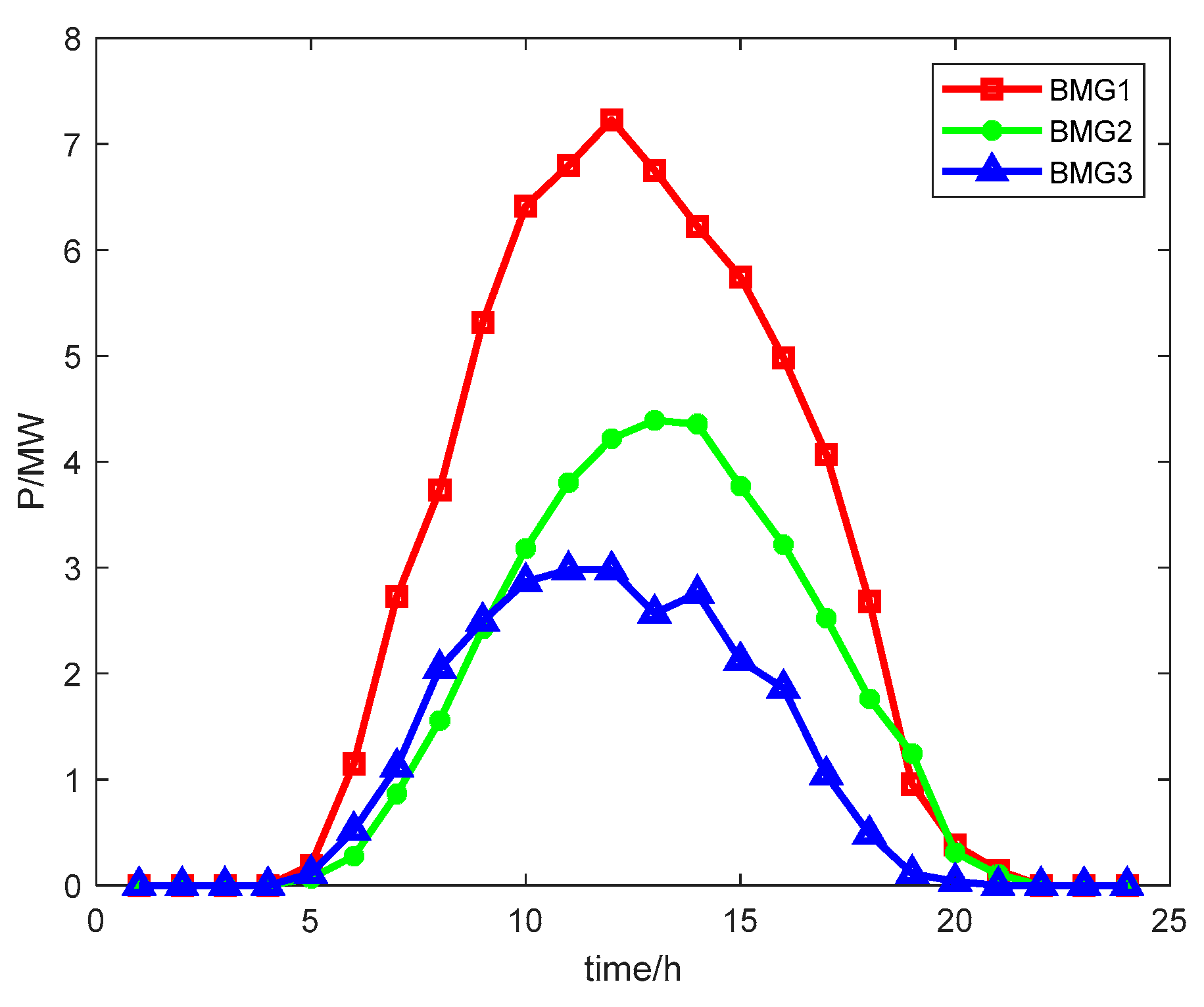
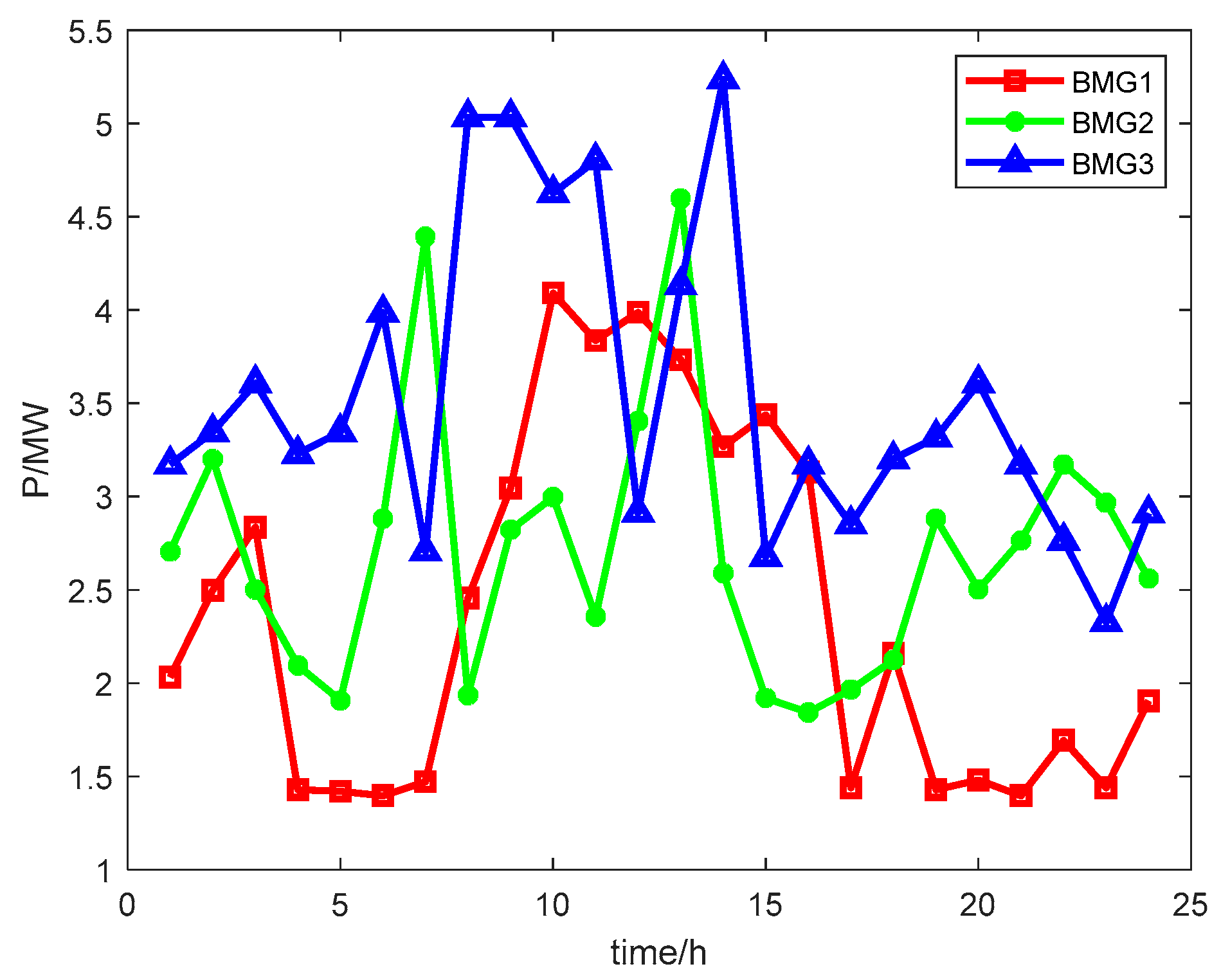
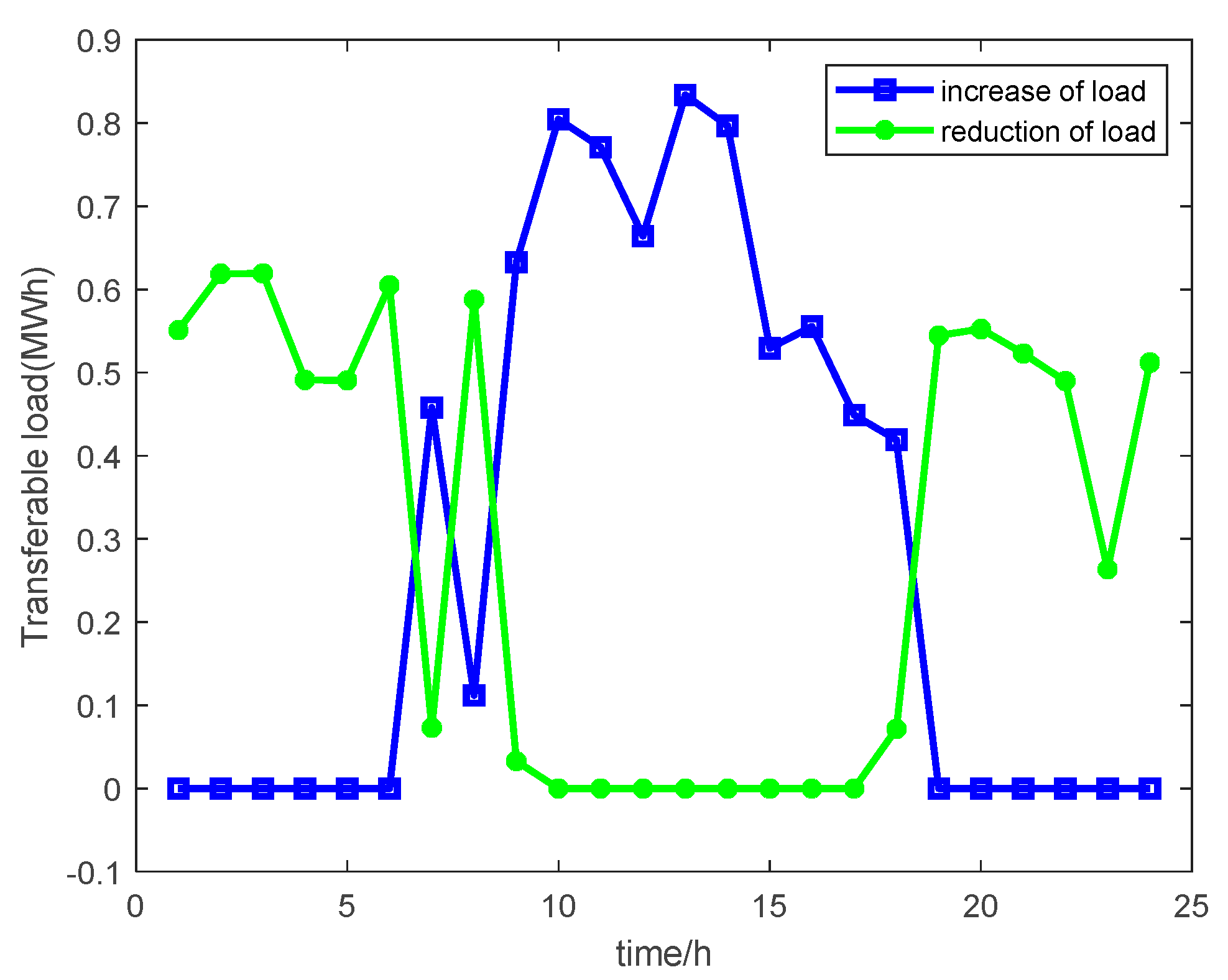
6.2.1. Analysis of Internal Energy Interaction Results of Multi-Building Microgrid

As a leader in the MBMG internal energy market, the DNO has the power to set internal electricity prices. The transaction prices between the DNO and various building microgrid users are shown in Figure 8.
In the MBMG internal energy market, a BMG, as a follower, adjusts its own energy scheduling based on the internal electricity price. The charging and discharging of energy storage for each building microgrid user and the MBMG transferable load are shown in Figure 9 and Figure 10.
As can be seen from Figure 6, Figure 7, Figure 8, Figure 9 and Figure 10, when photovoltaic power generation is almost zero (0:00–6:00, 20:00–24:00), supply is less than demand and electricity prices are high. Building microgrid users adjust their own power consumption strategies (that is, increase the amount of energy stored and reduce load usage) to reduce their own operating costs. During the period of rising photovoltaic power generation (6:00–12:00), supply exceeds demand, and multi-building microgrid photovoltaic power generation is sufficient to maintain internal power demand. The DNO also does not need to purchase power from the superior grid, resulting in a significant and continuous decline in electricity prices. Building microgrid users regulate their own power consumption strategies (namely, energy storage does not operate, increasing load usage) to achieve maximum benefits. During the period near the peak of photovoltaic power generation (12:00–15:00), the usage load of BMG2 and BMG3 suddenly increases, and the SDR decreases, resulting in a rapid ascent in electricity prices. In order to maintain their own interests, building microgrid users adjust their own electricity consumption strategies (namely, reducing the amount of charging stored energy and the amount of load usage) to increase the SDR, resulting in a rapid decline in electricity prices. During the period of continuous decline in photovoltaic power generation (15:00–20:00), when supply is less than demand, the DNO needs to purchase power from the superior power grid, leading to a significant and sustained increase in electricity prices. Building microgrid users modify their own power consumption strategies (namely, reducing the amount of energy stored and the amount of load used) to reduce operating costs. In summary, through the market game between the DNO and MBMGs, the utilization rate of distributed energy has been significantly improved, reducing the adverse impact of the strong randomness of distributed energy. At the same time, the pricing mechanism based on SDR has been established, using electricity prices to promote the participation of building microgrid users in energy scheduling, effectively preventing operational security issues, such as line congestion, that may occur during peak periods of power consumption and issues such as low energy utilization caused by low peak periods of power consumption; it also further enhances the economy of overall operation.

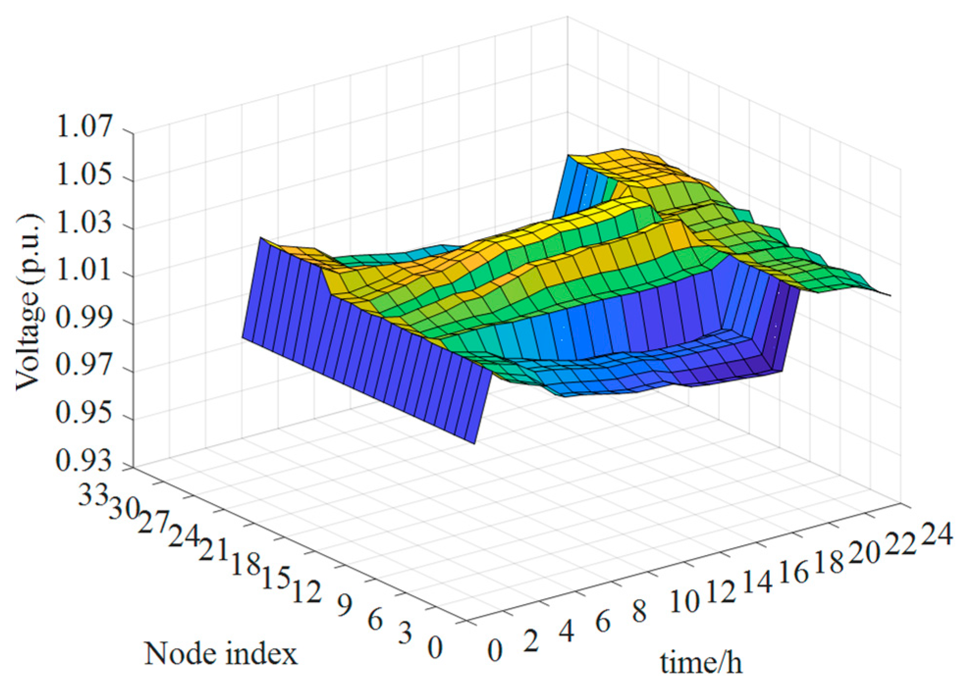
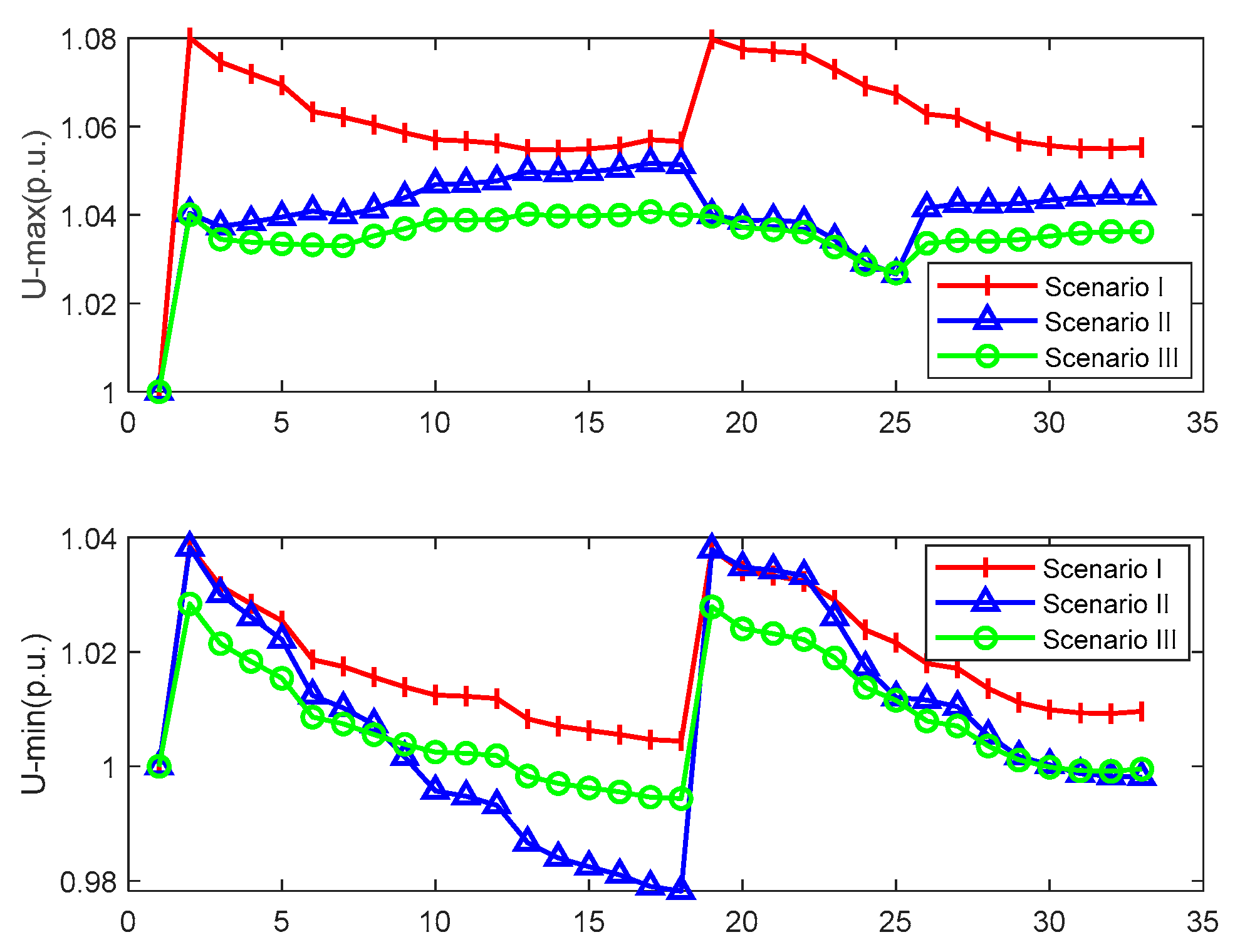
6.2.2. Voltage Stability Analysis

The node voltage of a multi-building microgrid system is obtained by solving a master–slave game-based comprehensive decision-making model for the multi-building microgrid distribution system, where each node voltage meets the network power flow constraints of the DN in the upper DNO security economic decision-making model. The 24 h voltage of each node in a multi-building microgrid system is shown in Figure 11. It can be found that the voltage per unit value of each node is between 0.96 and 1.04, which meets the safety index requirements of flexible distribution systems and effectively reduces the impact of voltage fluctuations on the system.

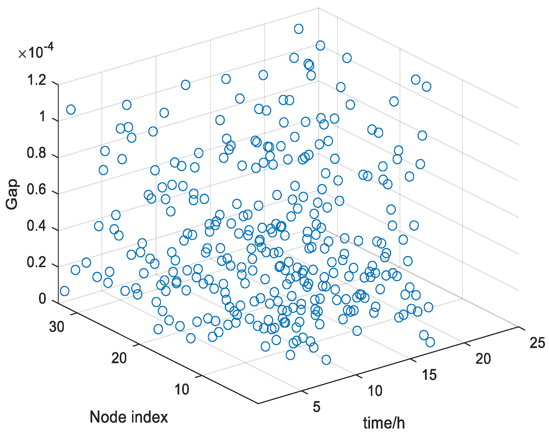
6.2.3. Model Validation Analysis

The accuracy of the convex relaxation proposed in this paper is verified by the defined gap value. The 24 h gap value of a multi-building microgrid system is shown in Figure 12. It can be found that the overall error value of the multi-building microgrid system is less than 1.2 × 10⁻⁴, so the convex relaxation is accurate.

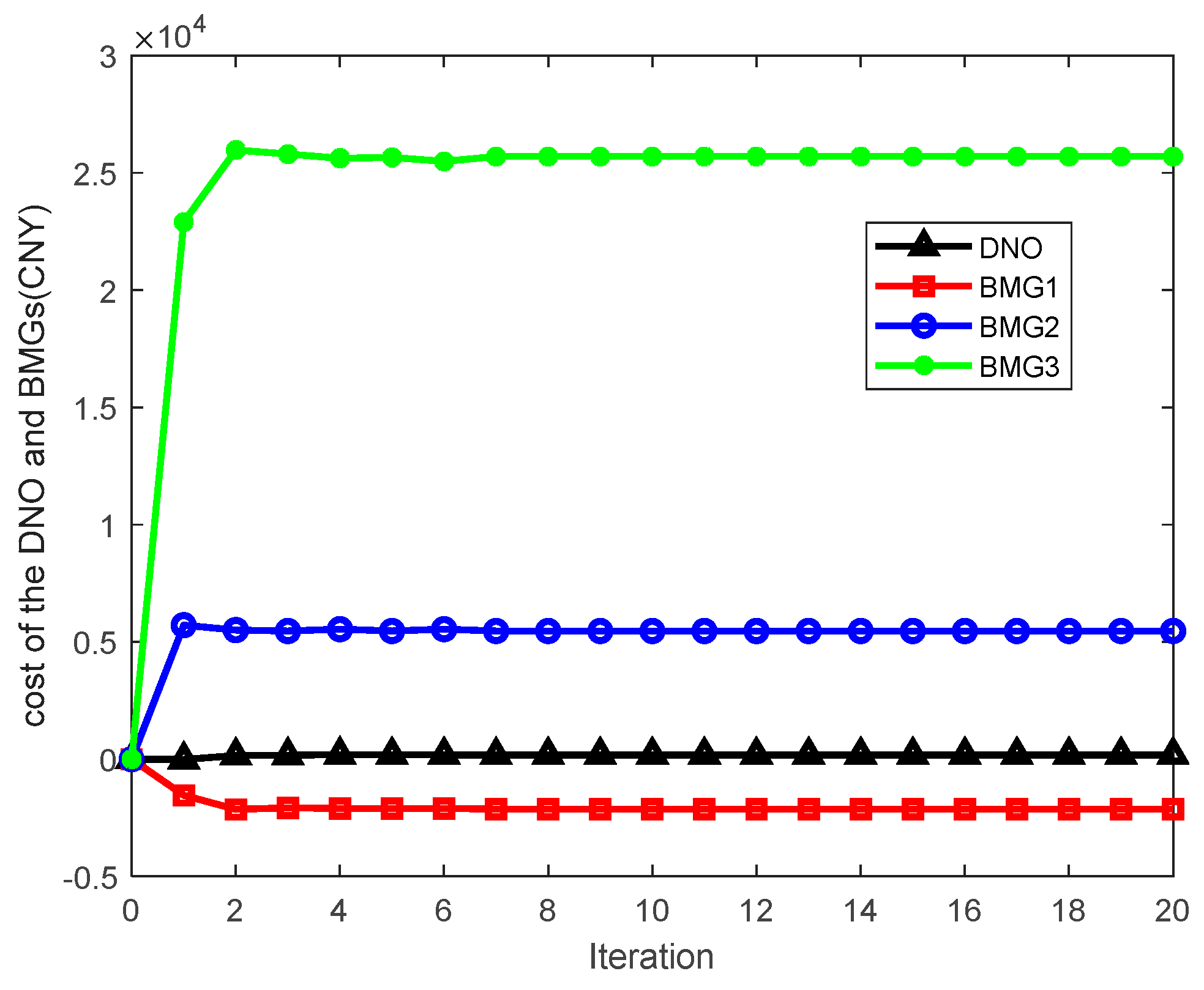
6.2.4. Model Convergence Analysis

Twenty iterative solutions are performed in this article to verify the effectiveness of the iterative search method. Figure 13 shows the relationship between DNO benefits and the number of iterations for each BMG. It can be observed that each parameter quickly converges to the equilibrium point, where the costs of the DNO begin to converge at the eighth iteration and the costs of BMG begin to converge at the seventh iteration, verifying the effectiveness of the method.

6.3. Comparative Analysis of Cases

To verify the effectiveness of the decision-making methods proposed in this article, this section compares and analyzes them with the other two different scenarios. The specific scenarios are described as follows:
Scenario I: The existing distribution system energy interaction control, aimed at maximizing economic efficiency, does not encompass safety factors such as power flow, line power losses, and voltage deviations [5].
Scenario II: Soft Open Points are not installed on the basis of the scenario proposed in this article.
Scenario III: The method proposed in this article.
Through simulation analysis of the three scenarios, the comparison results of system-related performance data or voltage values are shown in Table 3 and Figure 14.
In terms of Scenario III, the output of the active/reactive power of the SOPs at each time period is shown in Figure 15. SOP1 connects building microgrid 1 and building microgrid 3, SOP2 connects building microgrid 1 and building microgrid 2, and SOP3 connects building microgrid 2 and building microgrid 3.
From the data in Table 2, it can be seen that for Scenario I, due to its goal of maximizing economic benefits without considering safety factors, ESSs and transferable loads are fully regulated to achieve maximum benefits, reducing the operating costs of each BMG. However, their active power losses and voltage fluctuations are significantly greater than those of Scenario III, posing serious security risks to the actual operation of the DN and even causing interruption of power trading. In addition, large active power losses and voltage fluctuations lead to an imbalance in revenue between the DNO and each BMG, making it impossible to maximize the economic benefits of the entire distribution system.
Comparing Scenario II with Scenario III, it can be found that line loss and operating costs have obviously increased without SOPs. At the same time, combining Figure 11 and Figure 14, It can be observed that in terms of system safety performance, SOPs can quickly adjust system power to reduce voltage fluctuations, eliminate the issue of voltage overrun, and maintain the voltage amplitude within the safe operating range ([0.96, 1.04] p.u.), which proves that SOPs can improve the effectiveness of the safety performance of power distribution systems. In addition, combining Figure 9, Figure 10 and Figure 15, it can be found that at the level of power trading, the SOP active power control situation is consistent with the actions of energy storage charging and discharging and the transferable load actions of each building microgrid, reflecting that SOPs can quickly ameliorate the active power flow distribution of MBMGs in real time through their association with the DNO, providing a new optimization path for MBMG power trading. SOPs upgrade the transaction environment and avoid transaction delay or failure caused by line blockage. They enable the regional building microgrid to complete the power transaction in time, quickly eliminating the tide fluctuation caused by the DG, which indirectly boosts the economy of MBMG operation.
To sum up, the comparison can verify that the strategy proposed in this paper elevates the security performance of the system, balances the economic interests of the main players in the multi-building microgrid system, and provides a more efficient and economical solution to promote the consumption of local distributed energy.

7. Conclusions

This paper delves into the competitive dynamics within MBMG system transactions. Through a comprehensive analysis of market factors encompassing the DNO, building microgrid users, SOP utilization, and distributed energy storage, it introduces an integrated interactive control method of MFDS based on a master–slave game theory. The key findings can be summarized as follows:
(1)
In contrast to the traditional operational mode of multi-building microgrids (MBMGs), the transaction strategy proposed in this paper, grounded in the principle of master–slave games, takes into account bidirectional trading between the central power grid and the MBMG system. This strategy not only fosters the utilization of locally distributed energy but also optimizes the interests of all stakeholders involved in the game;
(2)
Adopting an SDR-based pricing mechanism has spurred the active engagement of building microgrid users in energy regulation. This has accelerated economic benefits for all participants and bodes well for the sustained operation of the MBMG system;
(3)
In contrast to approaches solely focused on economic benefits, the integrated interactive control method of multi-agent flexible distribution systems presented in this paper, albeit resulting in a marginal increase in building microgrid operational costs, yields substantial reductions in active power losses and minimizes voltage fluctuations from the perspective of the overall MBMG system; this enables transactions between building microgrid users and the DNO to occur more quickly and securely. Over the long term, this methodology substantially diminishes the overall power grid’s operating expenses, ensuring overall economic viability;
(4)
Relative to alternative operational strategies for MBMG systems, this article introduces Soft Open Points (SOPs) between building microgrids, significantly enhancing the flow of active and reactive power. From a physical perspective, although the incorporation of SOPs results in additional power losses and heightened operational costs for the DNO, they significantly bolster the system’s safety performance; this translates to reduced power losses across the system, lower total operating costs for the DNO, and indirect safeguarding of its economic interests. From an economic standpoint, they have notably transformed the trading environment, amplified the internal transaction flexibility within MBMG systems, and trimmed operating costs for all participating stakeholders.

Author Contributions

Project administration and funding acquisition, W.L.; methodology, S.Z.; writing—original draft, B.X.; resources and supervision, T.Z.; data curation and writing—review editing, L.S.; visualization, M.W.; software, X.W. All authors have read and agreed to the published version of the manuscript.

Funding

The project is supported by the Science and Technology Project of State Grid Anhui Electric Power Co., Ltd., China (52120523001A).

Data Availability Statement

Some or all of the data, models, or code generated or used during this study can be obtained from the corresponding authors upon request.

Conflicts of Interest

The authors declare that they have no known competing financial interest or personal relationship that could have appeared to influence the work reported in this paper. Wei Lou is employee of the Science and Technology Project of State Grid Anhui Electric Power Co., Ltd., China, who provided funding and teachnical support for the work. The funder had no role in the design of the study; in the collection, analysis, or in-terpretation of data, in the writing of the manuscript, or in the decision to publish the results.

References

  1. Dong, Y.; Yang, T.; Liu, P.; Xu, Z. Comparing the Standards of Life Cycle Carbon Assessment of Buildings: An Analysis of the Pros and Cons. Buildings 2023, 13, 2417. [Google Scholar] [CrossRef]
  2. Jia, H.; Yang, Q.; Jiang, Z.; Chen, W.; Zhou, Q. AppSimV: A Cyber–Physical Simulation and Verification Platform for Software Applications of Intelligent Buildings. Buildings 2023, 13, 2404. [Google Scholar] [CrossRef]
  3. Zhou, B.; Peng, H.; Zang, T. A Point to Point Trading Strategy Based on Stackelberg Game in multi-microgrid systems. J. Electr. Power Syst. Autom. 2023, 35, 103–111. [Google Scholar] [CrossRef]
  4. Zhou, Q.; Shahidehpour, M.; Alabdulwahab, A.; Abusorrah, A. Flexible division and unification control strategies for resilience enhancement in networked microgrids. IEEE Trans. Power Syst. 2020, 35, 474–486. [Google Scholar] [CrossRef]
  5. Liu, Z.; Wang, L.; Ma, L. A transactive energy framework for coordinated energy management of networked microgrids with distributionally robust optimization. IEEE Trans. Power Syst. 2020, 35, 395–404. [Google Scholar] [CrossRef]
  6. Jadhav, A.M.; Patne, N.R.; Guerrero, J.M. A novel approach to neighborhood fair energy trading in a distribution network of multiple microgrid clusters. IEEE Trans. Ind. Electron. 2019, 66, 1520–1531. [Google Scholar] [CrossRef]
  7. Anoh, K.; Maharjan, S.; Ikpehai, A.; Zhang, Y.; Adebisi, B. Energy peer-to-peer trading in virtual microgrids in smart grids: A game-theoretic approach. IEEE Trans. Smart Grid 2020, 11, 1264–1275. [Google Scholar] [CrossRef]
  8. Esfahani, M.M.; Hariri, A.; Mohammed, O.A. A multiagent-based game-theoretic and optimization approach for market operation of multi-microgrid systems. IEEE Trans. Ind. Inform. 2019, 15, 280–292. [Google Scholar] [CrossRef]
  9. Park, S.; Lee, J.; Bae, S.; Hwang, G.; Choi, J.K. Contribution-Based Energy-Trading Mechanism in Microgrids for Future Smart Grid: A Game Theoretic Approach. IEEE Trans. Ind. Electron. 2016, 63, 4255–4265. [Google Scholar] [CrossRef]
  10. Ji, H.; Wang, C.; Li, P.; Ding, F.; Wu, J. Robust operation of soft open points in active distribution networks with high penetration of photovoltaic integration. IEEE Trans. Sustain. Energy 2019, 10, 280–289. [Google Scholar] [CrossRef]
  11. Yan, M.; Shahidehpour, M.; Paaso, A.; Zhang, L.; Alabdulwahab, A.; Abusorrah, A. Distribution Network-Constrained Optimization of Peer-to-Peer Transactive Energy Trading Among Multi- microgrids. IEEE Trans. Smart Grid 2021, 12, 1033–1047. [Google Scholar] [CrossRef]
  12. Wang, Y.; Huang, Z.; Shahidehpour, M.; Lai, L.L.; Wang, Z.; Zhu, Q. Reconfigurable Distribution Network for Managing Transactive Energy in a Multi-Microgrid System. IEEE Trans. Smart Grid 2019, 11, 1286–1295. [Google Scholar] [CrossRef]
  13. Yang, Z.; Hu, J.; Ai, X.; Wu, J.; Yang, G. Transactive Energy Supported Economic Operation for Multi-Energy Complementary Microgrids. IEEE Trans. Smart Grid 2020, 12, 4–17. [Google Scholar] [CrossRef]
  14. Song, Y.; Sun, C.; Li, P.; Yuan, K.; Song, G.; Wang, C. SOP based supply restoration method of active distribution networks using soft open point. Proc. CSEE 2018, 38, 4390–4398. (In Chinese) [Google Scholar]
  15. Yu, Y.; Li, G.; Li, Z. A game theoretical pricing mechanism for multi- microgrid energy trading considering electric vehicles uncertainty. IEEE Access 2020, 8, 156519–156529. [Google Scholar] [CrossRef]
  16. Paudel, A.; Chaudhari, K.; Long, C.; Gooi, H.B. Peer-to-peer energy trading in a prosumer based community microgrid: A game-theoretic model. IEEE Trans Ind. Electron. 2019, 66, 6087–6097. [Google Scholar] [CrossRef]
  17. Zhou, Y.; Wu, J.; Long, C.; Ming, W. State-of-the-art analysis and perspectives for peer-to-peer energy trading. Engineering 2020, 6, 739–753. [Google Scholar] [CrossRef]
  18. Zhang, C.; Wu, J.; Zhou, Y.; Cheng, M.; Long, C. Peer-to-Peer energy trading in a microgrid. Appl. Energy 2018, 220, 15. [Google Scholar] [CrossRef]
  19. Contreras, J.; Klusch, M.; Krawczyk, J. Numerical solutions to Nash-Cournot equilibria in coupled constraint electricity markets. IEEE Trans Power Syst. 2004, 19, 195–206. [Google Scholar] [CrossRef]
  20. Lee, W.; Xiang, L.; Schober, R.; Wong, V.W.S. Direct Electricity Trading in Smart Grid: A Coalitional Game Analysis. IEEE J. Sel. Areas Commun. 2014, 32, 1398–1411. [Google Scholar] [CrossRef]
  21. Chis, A.; Koivunen, V. Coalitional game-based cost optimization of energy portfolio in smart grid communities. IEEE Trans Smart Grid 2019, 10, 1960–1970. [Google Scholar] [CrossRef]
  22. Xu, Q. Algorithm design of equilibrium bidding strategy in bargaining game. Comput. Eng. Appl. 2020, 56, 170–175. [Google Scholar]
  23. Li, P.; Ji, H.; Wang, C.; Zhao, J.; Song, G.; Ding, F.; Wu, J. Coordinated Control Method of Voltage and Reactive Power for Active Distribution Networks Based on Soft Open Point. IEEE Trans. Sustain. Energy 2017, 8, 1430–1442. [Google Scholar] [CrossRef]
  24. Wang, C.; Sun, C.; Li, P.; Wu, J.; Xing, F.; Yu, Y. Optimization and Analysis of Distribution Network Operation Based on SNOP. Power Syst. Autom. 2015, 39, 82–87. [Google Scholar]
  25. Yang, X.; He, H.; Zhang, Y.; Chen, Y.; Weng, G. Interactive Energy Management for Enhancing Power Balances in Multi-Microgrids. IEEE Trans. Smart Grid 2019, 10, 6055–6069. [Google Scholar] [CrossRef]
  26. Farivar, M.; Low, S.H. Branch flow model: Relaxations and convexification (part I). IEEE Trans. Power Syst. 2013, 28, 2554–2564. [Google Scholar] [CrossRef]
  27. Low, S.H. Convex relaxation of optimal power flow, I: Formulations and relaxations. IEEE Trans. Control Netw. Syst. 2014, 1, 15–27. [Google Scholar] [CrossRef]
  28. Liu, N.; Yu, X.; Wang, C.; Li, C.; Ma, L.; Lei, J. Energy-Sharing Model with Price-Based Demand Response for Microgrids of Peer-to-Peer Prosumers. IEEE Trans. Power Syst. 2017, 32, 3569–3583. [Google Scholar] [CrossRef]
  29. Gans, J.; King, S.; Stonecash, R.; Mankiw, N.G. Principles of Economics; Cengage Learning: Melbourne, Australia, 2011. [Google Scholar]
  30. Cruz, M.R.; Fitiwi, D.Z.; Santos, S.F.; Mariano, S.J.; Catalao, J.P. Multi-Flexibility Option Integration to Cope With Large-Scale Integration of Renewables. IEEE Trans. Sustain. Energy 2020, 11, 48–60. [Google Scholar] [CrossRef]
  31. Li, Y.; Feng, C.; Wen, F.; Wang, K.; Huang, Y. Energy Pricing and Management for Park-level Energy Internets with Electric Vehicles and Power-to-gas Devices. Autom. Electr. Power Syst. 2018, 42, 1–10. [Google Scholar]
  32. Sun, F.; Ma, J.; Yu, M. The Day-Ahead and Intraday Coordinated Energy Management Method for Active Distribution Networks Based on Multi-Terminal Flexible Distribution Switch. Proc. CSEE 2020, 40, 778–790. [Google Scholar]
Figure 1. MFDS interactive framework.
Buildings 14 00325 g001
Figure 2. The master–slave game architecture of the DNO and MBMG.
Buildings 14 00325 g002
Figure 3. The relationship between the internal prices and the SDR.
Buildings 14 00325 g003
Figure 4. Game-solving flowchart.
Buildings 14 00325 g004
Figure 5. The modified IEEE 33-node system.
Buildings 14 00325 g005
Figure 6. Prediction of PV output of each building microgrid.
Buildings 14 00325 g006
Figure 7. Load demand forecast for each building microgrid.
Buildings 14 00325 g007
Figure 8. Dynamic diagram of internal sales and purchase price.
Buildings 14 00325 g008
Figure 9. Dynamic diagram of energy storage charge and discharge for each building microgrid.
Buildings 14 00325 g009
Figure 10. MBMG transferable load dynamic diagram.
Buildings 14 00325 g010
Figure 11. Three-dimensional diagram of system voltage.
Buildings 14 00325 g011
Figure 12. Gap value chart.
Buildings 14 00325 g012
Figure 13. Iteration times graph of the DNO and BMGs.
Buildings 14 00325 g013
Figure 14. Comparison of maximum and minimum voltage values under three scenarios.
Buildings 14 00325 g014
Figure 15. The output of active/reactive power of the SOPs.
Buildings 14 00325 g015
Table 2. IEEE 33 bus test system-related parameters.
EntityEquipmentLocationParameters
BMG1PVNode24400 kW
ESSNode231.0 MWh, 0.2 MW, 0.95
BMG2PVNode27400 kW
ESSNode321.0 MWh, 0.2 MW, 0.95
BMG3PVNode7,10500 kW, 500 kW
ESSNode111.0 MWh, 0.2 MW, 0.95
DNSOPsNode12–22,25–29,18–33Capacity: 1.0 WVA
OLTCNode1-2±5 × 1% (includes 0 × 1%)
Table 3. Comparison results under different scenarios.
System PerformanceScenario IScenario IIScenario III
Line power loss (kWh)639.8311420.947632.714
SOP power loss (kWh)408.7940403.394
DNO cost (USD)−323.921136.216−186.5302
The total cost of building microgrid cluster (USD)29,022.21629,363.34729,033.107
Disclaimer/Publisher’s Note: The statements, opinions and data contained in all publications are solely those of the individual author(s) and contributor(s) and not of MDPI and/or the editor(s). MDPI and/or the editor(s) disclaim responsibility for any injury to people or property resulting from any ideas, methods, instructions or products referred to in the content.

