Abstract
The accurate prediction of residential heat load is crucial for effective heating system design, energy management, and cost optimization. In order to further improve the prediction accuracy of the model, this study introduced principal component analysis (PCA), the minimum sum of squares of the combined prediction errors (minSSE), genetic algorithm (GA), and firefly algorithm (FA) into back propagation (BP) and ELMAN neural networks, and established three kinds of combined prediction models. The proposed methodologies are evaluated using real-world data collected from residential buildings over a period of one year. The obtained results of the PCA-BP-ELMAN, FA-ELMAN, and GA-BP models are compared with the neural network before optimization. The experimental results show that the combined prediction models have higher prediction accuracy. The Mean Absolute Percentage Error (MAPE) evaluation indices of the three combined models are distributed between 5.95% and 7.05%. The FA-ELMAN model is the combination model with the highest prediction accuracy, and its MAPE is 5.95%, which is 2.25% lower than the MAPE of an individual neural network. This research contributes to the field by providing a comprehensive and effective framework for residential heat load prediction, which can be valuable for building energy management and optimization.
1. Introduction
Currently, the proportion of energy consumption in the construction sector in our country’s total energy consumption has reached 30%, and the energy consumption generated by heating accounts for 25% of the total energy consumption in buildings [1]. As of 2020, the national coverage of centralized heating has reached 12.266 billion square meters. However, the increase in carbon emissions and pollutant emissions caused by fuel combustion has resulted in serious environmental problems. In order to alleviate the energy crisis and improve environmental pollution, the government has implemented numerous measures in energy conservation and emission reduction. In our country, heating systems are mainly regulated through manual experience. However, due to the characteristics of centralized heating systems, such as significant time delays, strong non-linearity, high energy consumption, and multiple influencing factors, the traditional inefficient heating regulation model has created issues such as significant heat waste and uneven distribution of heating. In practice, the energy consumption in heating processes still cannot meet the heating needs of users. Therefore, it is necessary to incorporate heat load forecasting into the heating system to guide heating operations. By utilizing a heat load prediction model, the heating system can adjust in advance based on the predicted load. Building an accurate, efficient, and reliable heat load prediction model is crucial in ensuring the centralized heating system can meet heating demands effectively and on demand.
The commonly used heat load predicting models include the data-driven model and mechanism model. By using building energy simulation software such as EnergyPlus V22 and TRNSYS 18 to evaluate building heat load, the mechanism model requires a complex calculation process and usually takes a long time to get the result, so it is not suitable for real-time energy consumption prediction [2,3]. However, the data-driven model can produce prediction results in a relatively short time, which is suitable for real-time energy consumption prediction and rapid decision-making. Common data-driven models used in various fields include statistical analysis techniques, machine learning algorithms, and deep learning architectures. Statistical methods tend to overfit when handling diverse influencing factors, leading to poor predictive performance of the models [4,5,6,7]. With the wide application of artificial intelligence algorithms in the prediction field [8,9,10,11], more and more scholars have started researching load-predicting methods founded on machine learning [12,13,14]. Some commonly used approaches in machine learning include artificial neural networks (ANN) [15], support vector machines [16], extreme learning machines [17], random forest (RF) [18], and regression trees [19]. Park et al. [20] separately used partial least squares, neural networks, and support vector regression (SVR) to establish load forecasting models for district heating, and the research results showed that SVR had the lowest average relative error. Meng et al. [21] built an ELMAN neural network prediction model and, on this basis, proposed a DR control strategy for office buildings. Wang et al. [22] implemented 12 models for single-building heat load predicting, discussing the impact of prediction level and input uncertainty on load forecasting accuracy. Introducing these models for heat load forecasting has provided good predictive results, demonstrating that an individual model based on machine learning can derive feasible computational rules from a significant volume of historical operational data.
Several researchers have adopted hybrid methods that combine an optimization algorithm with a machine-learning model [23]. In an improved model, various parameters can be optimized, such as weights, bias, and others [24]. The combination models can be divided into two classifications. The initial classification is the ensemble models that combine multiple individual models [25]. These models are trained on the same dataset using different individual models. The predictions from each individual model are then combined to generate an optimal output. The second category is the improved models that combine an individual model with optimization methods. For example, Fan et al. [18] developed an integrated model for predicting commercial building loads. They used a genetic algorithm (GA) to optimize the weights of the eight prediction models and combined the results to obtain the final prediction. The experimental results showed that the ensemble model outperformed typical individual models in terms of prediction accuracy. Qi et al. [26] introduced GA into a back propagation (BP) neural network to establish a heat load prediction model. Meanwhile, the date type was quantified when selecting input variables, which ensured the prediction accuracy. Principal component analysis (PCA) was used to obtain reasonable model inputs and build a prediction model [27]. Zhao et al. [28] proposed a convolutional neural network (CNN) hybrid short-term heat load prediction model based on the adaptive T-distribution satin Bowerbird algorithm. Compared with other prediction models, The Mean Absolute Percentage Error (MAPE) and Root Mean Square Error (RMSE) of the mixed model decreased by 18.08% and 16.26%, respectively. Song et al. [25] proposed a heat load prediction model based on convolution neural network-long short-term memory (CNN-LSTM), which obtains a more accurate dynamic heat load model. Al-shammari et al. [29] proposed an SVR regional heating system thermal load prediction model based on the firefly algorithm (FA).
In the field of heat load prediction, the innovation of this research lies in combining optimization algorithms with machine learning models to improve the accuracy and reliability of heat load prediction by comparing the predicting performance of different combination models. The heat load prediction models of PCA-BP-ELMAN, FA-ELMAN, and GA-BP were established, respectively. We used the real heat load data and MATLAB platform for experimental simulation. By comparing and analyzing the performance of different combined prediction models, we explore the effectiveness and applicability of the combination of optimization algorithm and machine learning model in heat load prediction and determine the best-combined model to provide more accurate and reliable heat load prediction.
2. Methods
The research framework, depicted in Figure 1, encompasses key components such as data collection, data preprocessing, feature selection, implementation, and prediction of classical individual machine learning models, as well as the implementation and prediction of combined models. To evaluate model performance, four evaluation indicators are employed to identify an individual model with superior predictive capabilities. Building upon this, PCA, minSSE algorithm, GA, and FA are incorporated into multiple efficient individual models for heat load prediction, resulting in the creation of three combined models. These models are assessed using the generated dataset and compared with both the pre-optimized prediction model and different combined models to validate the superior prediction accuracy of the combined models. Furthermore, the study investigates the optimization effects of various combination methods.
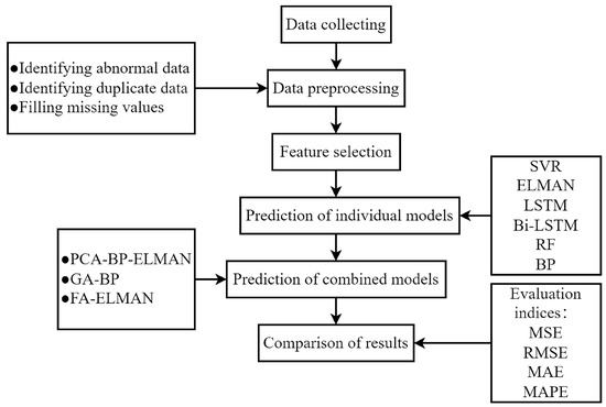
Figure 1.
Research framework of this study.
2.1. Optimization Algorithm
2.1.1. Principal Component Analysis
The heating load is influenced by various factors, including meteorological, system, social, and building factors [30]. However, considering all these factors comprehensively when calculating it can lead to increased complexity and difficulty in problem-solving. PCA offers a solution by reducing multiple initial indicators that affect the problem to a few major components that are most effective. This simplifies the problem analysis [31,32]. The main steps of this method include:
- (1)
- The n samples with m influencing factors are subjected to data standardization, then:
- (2)
- The eigenvalues and eigenvectors of the correlation coefficient matrix are calculated, where rij represents the correlation coefficient between the ith and jth influencing factors. A higher value indicates a stronger correlation between the two factors. To calculate the correlation coefficient, use the Equation (4) and sort the eigenvalues in descending order, λ1, λ2, …, λm. From these feature vectors, m new index vectors can be formed, as shown in Equation (5):
- (3)
- The contribution rate is calculated, and the principal component is extracted.
2.1.2. The minSSE Algorithm
The model is built by assigning distinct weight coefficients to the predictions generated by multiple individual models. Subsequently, a new predicted value is derived through the employment of the weighted average method. The main focus of the combined model lies in identifying the weight coefficient for each model, and there exist numerous calculation methods that can be utilized for this purpose. This study utilizes the minSSE algorithm, which aims to minimize the sum of squares of the combined prediction error. By applying this algorithm, the optimal weight coefficient can be determined.
Define the actual value at time t as xt, t = 1, 2, …, p; Define the prediction of the ith model as xit, i = 1, 2, …, n; t = 1, 2, …, p; Let {l1, l2, …, ln} denote the weight coefficients of the n models, and these coefficients must satisfy the following requirements.
as the predicted value of the combined model at time t is calculated as follows:
The calculation process of the minSSE algorithm is as follows:
- (1)
- The prediction error of the combined prediction model at time t is calculated.
- (2)
- The combined prediction errors, denoted as et, are squared, and then summed to calculate the value of J.
Let L = , E = , J = LTEL
- (3)
- Let H = [1KK1]T; The following optimization model is constructed with the minimum sum of squares of prediction errors as the optimal criterion.
- (4)
- The Lagrange multiplier method is used to solve the model, and the optimal combinatorial weight vector L and the minimum sum of square of combinatorial prediction error J are obtained.
- (5)
- Based on the weight coefficients assigned to each individual model, the predicted value of the combined model is calculated.
2.1.3. The Genetic Algorithm
The steps involved in the GA primarily consist of population initialization, fitness function, selection, crossover, and mutation [33]. The following sections outline each step in detail:
- (1)
- Population initialization:
To facilitate computer recognition and storage, each individual in the population is encoded using a binary array. Each individual represents a real string consisting of four components: input layer and hidden layer link weight, hidden layer weight, hidden layer and output layer weight, and output layer weight.
- (2)
- Fitness function:
The fitness function is determined by the sum of squared errors between the predicted output value and the expected output value of the network. The calculation equation is as follows:
where n is the number of output nodes; yk is the expected value of the kth node of the BP neural network. Xk is the predicted value of the kth node.
- (3)
- Selection:
The roulette method, which employs a selection strategy based on the proportion of fitness values, is utilized for determining the selection probability (P) of each individual (i). This probability is calculated as follows:
where fi is the fitness of individual Xi; N is the number of population individuals.
- (4)
- Cross:
The process involves randomly selecting an individual chromosome from a set of chromosomes and crossing it over with another chromosome, employing a specific method to generate a novel individual.
- (5)
- Mutation:
The jth gene is selected for mutation in individual ith. At a particular locus, the gene is substituted with an allele, leading to the creation of a new individual.
2.1.4. The Firefly Algorithm
FA is a biologically inspired optimization algorithm that utilizes group search. Within a specified range, fireflies emit light randomly, and their attractiveness is directly proportional to the intensity of their light emissions. During the process of movement and aggregation, each firefly’s flight position changes based on the luminosity of the brightest individual in the current time zone. Ultimately, all fireflies converge towards the brightest individual.
The brightness function varying wi”h di’tance In Gaussian form is defined as:
where I0 is the maximum brightness of fireflies; d is the distance between two fireflies; γ is the absorption coefficient of light intensity.
The attractiveness function β(d) of a firefly at a distance reference point d is defined as:
where β0 is the attraction of fireflies at the light source.
For two fireflies located in wi and wj, the distance between them is expressed as:
where n is the dimension of the target problem; wi,k are the coordinates of the ith firefly on the k dimension; wj,k is the coordinates of the jth firefly on the k dimension.
When firefly I is attracted to another firefly j, which is brighter, the movement pattern is:
where α is the step factor; εi is the vector of random numbers derived based on a Uniform distribution or Gaussian distribution.
2.2. Construction of Models
2.2.1. Construction of Individual Models
- (1)
- SVR is a machine learning technique that is based on statistical learning theory and the principle of minimizing structural risk. Its primary objective is to prevent overfitting and ensure that the model can generalize and approximate accurately. SVR is particularly effective for identifying non-linear relationships between the dependent variable and multiple influencing factors, especially when working with limited sample sizes [34,35,36]. The essence is to project the training samples onto a high-dimensional plane and identify an appropriate hyperplane that can effectively separate the samples.
- (2)
- Elman neural network is a recurrent neural network composed of four layers. The input layer is responsible for signal transmission, while the output layer performs linear weighting. The hidden layer units are capable of employing either linear or non-linear transfer functions. The context layer is utilized to store the previous moment’s output values of the hidden layer units and subsequently feed them back to the network’s input [37].
- (3)
- LSTM is an improvement of recurrent neural networks (RNNs) that addresses the issue of long-term dependencies. It not only maintains the connectivity among hidden layer nodes in RNNs but also introduces the concept of filtering past states [38,39]. The results of long time series training with good continuity are better than those of ordinary RNN models [40,41]. The key to LSTM is the cell state, which carries pertinent information outward. The cell state undergoes updates through the forget gate, input gate, and output gate.
- (4)
- Based on LSTM, bidirectional long short-term memory (Bi-LSTM) transforms the single-direction LSTM layer into both Backward and Forward layers. The Forward layer processes the sequential information at the current time step, while the Backward layer reads the same sequence in reverse, incorporating the inverse order information. The final output combines the respective outputs from the Backward and Forward layers at each time step. In LSTM, the hidden output signals can be transmitted not only to neighboring grids but also to the next layer’s grids. During the training process, the two-state neurons do not interact, allowing for the expansion of the network into a typical feed-forward neural network. Building upon this, the adjustment of network weights is achieved through both forward and backward propagation methods [42,43].
- (5)
- RF is an improved algorithm of ensemble learning. It involves randomly sampling a training set of m samples, with replacement, from the original dataset. The size of the sample matches that of the original dataset. Then, it constructs m decision trees (where is an independently and identically distributed random vector). The final output of RF regression is obtained by averaging the outputs of the m decision trees.
- (6)
- BP neural network structure mainly consists of three layers: the input layer, the output layer, and the hidden layer. These layers are fully interconnected, and there is no coupling between neurons within the same layer. The network’s functionality is achieved through forward signal propagation and backward error propagation [44,45].
2.2.2. Construction of Combined Models
In order to improve the accuracy of artificial neural networks in building energy prediction, the following three problems need to be solved: First, it is easy to fall into the local optimal problem in the training stage; Secondly, the problem of input selection; Finally, the question of hyperparameter setting [46]. To solve the above problems, different optimization algorithms are introduced into building energy consumption prediction. The following is the construction process of the combined models.
- (1)
- PCA-BP-ELMAN
The parameters of the input layer were optimized using PCA, and the optimal weight coefficient of the model was obtained through the minSSE algorithm, which utilized the predicted and actual values of the BP and ELMAN neural network models. The PCA-BP-ELMAN model was then constructed based on these weight coefficients for prediction. The specific calculation process is depicted in Figure 2.
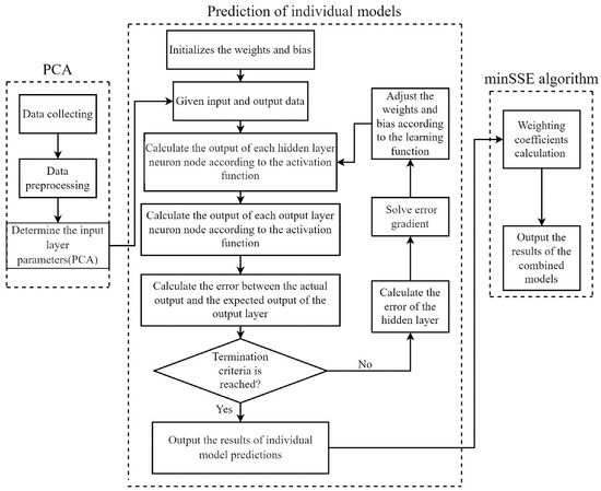
Figure 2.
A flowchart of the PCA-BP-ELMAN model.
- (2)
- FA-ELMAN
The optimal firefly individual is selected by changing the position and brightness of fireflies, followed by the optimal replacement of initial weights and bias [47]. The nonlinear relationship between each input parameter and the hourly heat load is established by the ELMAN neural network so as to enable accurate prediction. The ELMAN neural network is optimized by using FA, as shown in Figure 3.
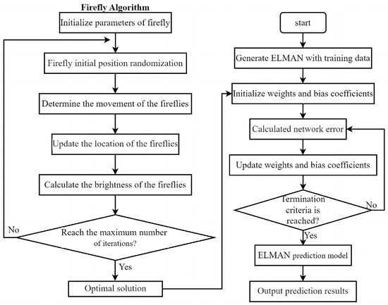
Figure 3.
A flowchart of the FA-ELMAN model.
- (3)
- GA-BP
GA is a methodology that simulates natural biological evolution and proves to be effective in solving complex problems, including nonlinear and global optimization [48]. In this study, GA is used to optimize the weights and bias of the BP neural network. Subsequently, the optimized weights and biases are employed to train the network and obtain the optimal solution. The specific calculation process is depicted in Figure 4.
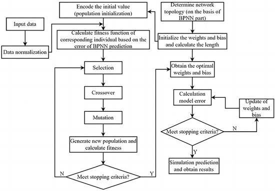
Figure 4.
A flowchart of the GA-BP model.
2.3. Data Processing and Analysis
2.3.1. Data Collecting and Preprocessing
Weifang City is located in the western part of the Shandong Peninsula and serves as a central city within the cluster. Geographically, it spans from 118°10′ to 120°01′ east longitude and 35°41′ to 37°26′ north latitude. The city covers a total land area of 1,616,723.99 hectares. Weifang experiences specific climatic conditions characterized by high winter temperatures, relatively abundant precipitation, and reduced sunlight. Overall, the climate is favorable. During the spring season, temperatures rise, precipitation increases, and sunlight is abundant, often leading to frequent meteorological disasters. In summer, the temperature becomes pleasant, with higher precipitation but less sunlight. Nevertheless, the climate remains suitable. In autumn, temperatures remain high, precipitation decreases slightly, and sunlight diminishes further. Weifang was selected as the research area for forecasting the heat supply load.
The data utilized in this study were obtained from two sources—the China Meteorological Data Network and the Weifang thermal data visualization monitoring platform. The dataset used for analysis was collected from a specific community. The type of enclosure structure is an ordinary external wall; the thickness of the wall is 240 mm, and the heat transfer coefficient is 2.03 W/m2/°C. The research focused on the complete heating season, with the query time range set from 15 November 2021, to 15 March 2022. To ensure data accuracy, a query interval of 3 min was used. Historical operating data and heat loads were sampled at 1-h intervals.
Since there are instances of abnormal and missing data, it is essential to apply proper data preprocessing techniques. For missing data, interpolation methods are used to fill in the gaps. Regarding abnormal data, the 3σ criterion is initially used to identify outliers, and then interpolation methods are employed to determine appropriate replacements. When long-term repetitions or omissions are detected, these occurrences are regarded as anomalies in the data-collection process and are subsequently eliminated.
2.3.2. Feature Selection
The heating load is affected by many factors, such as meteorological factors, system factors, social factors, and building factors. Temperature, relative humidity, wind speed, solar radiation, and other meteorological factors will affect the heating load. With the increase in temperature, the value of the heating load gradually decreases, and with the decrease in temperature, the value of the heating load gradually increases. When the temperature is unchanged, with the reduction of relative humidity, the evaporation of sweat is enhanced, the human body will feel cold, and the heating load will increase. As the wind speed increases, the heating load will also increase. Solar radiation also has a certain influence on the heating load. When the solar radiation is small, the heating load is larger, but its influence on the heat load is small. The influence of some characteristics of the heating network itself on the heat load is mainly reflected in the supply water temperature, return water temperature, circulation flow, and so on. Social factors such as residents’ heating habits, local policies, number of inhabitants, and development of the population will affect the change of heating load, and building factors such as its structure, function, geographical location, number of flats, the size of the heated volume and the quality of thermal insulation will also affect the heating load [30]. However, the influence of social factors on the heat load makes its change relatively slow, so it cannot be considered in the short-term heat load prediction, and once the building is formed, the influence of its own factors on the heat load can also be ignored.
To sum up, the preliminary analysis of the factors affecting heating load and the related literature review [49,50,51], Eight characteristics, including supply water temperature at time t-1, return water temperature at time t-1, heat load at time t-1, circulation flow at time t-1, solar radiation at time t-1, outdoor temperature at time t, wind speed at time t, and relative humidity at time t, were determined as input variables of the prediction model, and heat load at time t, were determined as output variables.
2.4. Evaluation Indices
The four selected accuracy evaluation indices for assessing the precision of the prediction model are as follows: Mean Square Error (MSE), RMSE, Mean Absolute Error (MAE), and MAPE [52].
where n—the number of samples; —the ith simulated value, GJ/h; —the ith actual measured value, GJ/h; —the mean of the simulated values, GJ/h; —the mean value of the measured value, GJ/h.
For the same dataset, smaller values of MSE, RMSE, MAE, and MAPE indicate reduced discrepancies between the predicted and actual values, implying a higher level of precision in the model.
3. Results
3.1. Comparisons of Individual Models
Using MATLAB as the calculation platform, the heat and meteorological data of a community in Weifang from 15 November 2021 to 15 March 2022 were used as training data to train the model. On this basis, the optimal input parameters of each model were selected as follows: (1). SVR: The kernel function is RBF, the loss function p = 0.4, the penalty factor C = 1000, and the kernel parameter γ = 0.01; (2). ELMAN: the number of neurons in the input layer is 8, the number of neurons in the output layer is 1, the number of neurons in the hidden layer is 8, the maximum number of iterations is 1000, the learning rate is 0.01, and the minimum error of the training target is 10−5; (3). LSTM and Bi-LSTM: The optimization method was the Adam algorithm, the maximum number of iterations was 300, the initial learning rate was 0.1, and the learning rate dropped to 0.1 × 0.1 after 50 training sessions. The optimized neural network was trained using the trainNet function. The model data is in a period of 24 h, and the input data formats are batch_size:24, time_step:1, iput_size:8; (4). RF: The number of decision trees is 500, the minimum number of leaves of each decision tree is 3, and the regRF_train function is called to train the model; (5). BP: Set the maximum number of iterations to 1000, the learning rate to 0.01, and the BP neural network structure to 8-14-1.
To assess the accuracy of these models, MSE, RMSE, MAE, and MAPE were used as evaluation indices, and their corresponding error indicators are presented in Table 1. The results in Table 1 indicate that the MAPE values for the RF, SVR, LSTM, and Bi-LSTM models are all greater than 15%. Moreover, as shown in Figure 5, these four models exhibit a significant deviation between the predicted and actual values, consistently overestimating the heat load. Consequently, these models demonstrate poor prediction performance and are not recommended for heat load prediction. Conversely, the BP and ELMAN neural network prediction models display lower evaluation indices with MAPE values less than 10%, MSE values below 0.1 GJ2/h2, RMSE values less than 0.3 GJ/h, and MAE values less than 0.2 GJ/h. Additionally, the predicted values from these two models exhibit minimal deviation from the actual values. Therefore, these models exhibit good prediction performance and are suitable for heat load prediction. Furthermore, in comparison to the other four models with inadequate prediction performance, the BP and ELMAN neural network models demonstrate a maximum reduction in MAPE of 20.5% and 19.75%, respectively.

Table 1.
Prediction results of the individual models.
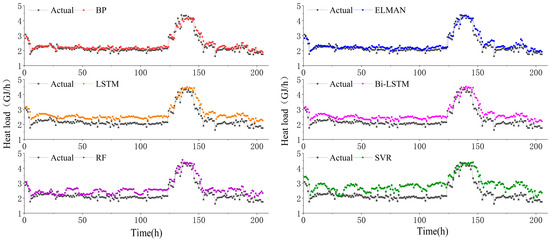
Figure 5.
Comparison of the performance between proposed and individual models.
3.2. Results of Combined Models
- (1)
- PCA-BP-ELMAN
To effectively reduce redundancy and correlation in the initial characteristic variable data for heat load prediction, dimensionality reduction processing was performed using IBM SPSS Statistics 26. The results, summarized in Table 2, showed that the first four principal components accounted for a cumulative contribution rate of 90.610%. This indicates that these principal components effectively captured and represented the majority of the information contained in the initial eight feature variables. As a result, principal components Y1 to Y4 were selected as the input data for further analysis.
Table 2.
The contribution rate of each component.
Table 3 presents the linear relationship between each principal component and its respective variable. In particular, principal component Y1, which accounts for a contribution rate of 45.684%, is largely associated with return water temperature, circulation flow rate, historical heat load, and outdoor temperature. Principal component Y2 is primarily linked to relative humidity and solar radiation. Additionally, principal components Y3 and Y4 are mainly influenced by wind speed and water supply temperature, respectively.
Table 3.
Principal component coefficient.
Each model in this study was trained using data that underwent PCA dimensionality reduction. The initial parameters for both the BP and ELMAN neural networks were set as follows: the transfer function was chosen as tansing, the training was conducted for 1000 iterations, the target error was defined as 10−5, the learning rate was set to 0.001, and the normalization range was [−1, 1]. The minSSE algorithm was employed to obtain the optimal weight coefficients for each model based on the predicted and actual values. Table 4 presents these weight coefficients, which range between 0 and 1, and their sum totals to 1.
Table 4.
Weighting coefficients of individual models.
Each individual model is used to predict the heat load, resulting in forecasted outcomes. These prediction results are then combined and weighted to calculate the final prediction results, which represent the prediction of the PCA-BP-ELMAN model. The respective evaluation indicators can be observed in Table 5, and a comparison between the predicted and actual results is presented in Figure 6.
Table 5.
Prediction results of the PCA-BP-ELMAN model.
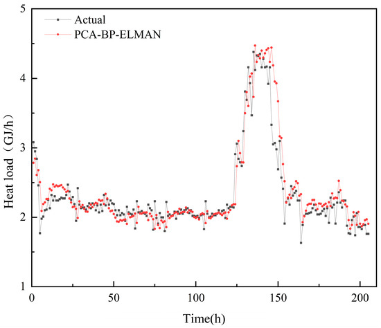
Figure 6.
Comparison between the actual data of heat load and results of a one-hour-ahead heat load prediction using the PCA-BP-ELMAN method.
- (2)
- FA-ELMAN
The initial parameters for the firefly algorithm are set as follows: a population size of 50, a maximum iteration limit of 30, a critical error threshold of 0.01, a maximum attraction value (β0) of 2, a light intensity absorption coefficient (γ) of 1, and a step factor (α) of 0.02. Similarly, the initial parameter settings for the ELMAN neural network are the same as described in the PCA-BP-ELMAN section. The respective evaluation indicators can be observed in Table 6, and a comparison between the predicted and actual results is presented in Figure 7.
Table 6.
Prediction results of the FA-ELMAN model.
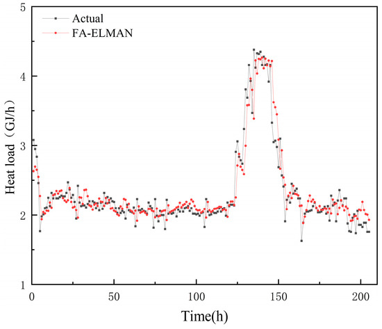
Figure 7.
Comparison between the actual data of heat load and results of a one-hour-ahead heat load prediction using the FA-ELMAN method.
- (3)
- GA-BP
The initial parameters for the genetic algorithm are set as follows: the number of iterations is 30, the population size is 10, the crossover probability is 0.8, and the mutation probability is 0.2. The initial parameter setting for the BP neural network section is the same as described in the PCA-BP-ELMAN method. The respective evaluation indicators can be observed in Table 7, and a comparison between the predicted and actual results is presented in Figure 8.
Table 7.
Prediction results of the GA-BP model.
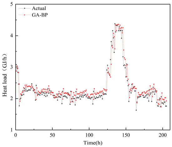
Figure 8.
Comparison between the actual data of heat load and results of a one-hour-ahead heat load prediction using the GA-BP method.
3.3. Comparisons of Individual and Combined Models
In order to analyze and compare the optimization effects of different combined prediction models, namely the BP and ELMAN neural network models, column charts and dot plots are utilized to assess the MSE, RMSE, MAE, and MAPE visually and effectively. These charts serve as clear and intuitive representations of the performance of the various models.
Figure 9 presents a comparison of evaluation errors between the BP model, ELMAN neural network model, and three combined prediction models. It is evident from the figure that the ELMAN neural network model exhibits the highest error index among the various prediction models, while the FA-ELMAN model shows the lowest error index. Additionally, the MSE, RMSE, MAE, and MAPE values of the three combined models consistently prove to be smaller than those of the traditional BP and ELMAN neural network models. This confirms the effectiveness of each employed optimization algorithm. Moreover, it is noteworthy that the model optimized by the FA algorithm demonstrates the most substantial reduction in each index, followed by the PCA-minSSE algorithm. Conversely, the model optimized by the GA algorithm displays the smallest reduction in each index. These findings suggest that the predictive performance of the three combined prediction models follows the order of FA-ELMAN, PCA-BP-ELMAN, and GA-BP, from high to low.
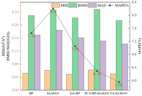
Figure 9.
Comparison performance of BP, ELMAN, and combined models.
The error-index of the FA-ELMAN combined prediction model (MSE = 0.046 GJ2/h2, RMSE = 0.214 GJ/h, MAE = 0.142 GJ/h, MAPE = 5.95%) was compared to that of the traditional ELMAN neural network model (MSE = 0.060 GJ2/h2, RMSE = 0.246 GJ/h, MAE = 0.184 GJ/h, MAPE = 8.20%). The results showed that the FA-ELMAN combined prediction model achieved significant improvements. Specifically, the MSE decreased by 0.014 GJ2/h2, the RMSE decreased by 0.032 GJ/h, the MAE decreased by 0.042 GJ/h, and the MAPE decreased by 2.25%.
4. Discussion
Accurate and reasonable heat load prediction models serve as a robust foundation for ensuring on-demand heating in centralized heating systems. In this study, we leverage winter heat load data from a residential building in Weifang City and integrate it with hourly meteorological data. This study primarily proposes three combined prediction models and examines the effectiveness of optimizing the combination of load prediction models, which improves the accuracy of heat load prediction. Nevertheless, further research can be undertaken in the following areas:
- (1)
- Due to data availability limitations, we can only use limited historical data for model training and validation. Therefore, further research may consider using longer time ranges of data as well as more frequent sampling to improve the generalization ability of the model.
- (2)
- The influence of indoor temperature and wind direction on heat load is disregarded due to limited data availability. Additionally, factors such as day-night variations, seasonal changes, and other potential influences are ignored to simplify the prediction model, owing to the complexity of its design. To address these limitations, future studies should expand the range of collected data by enhancing monitoring conditions. Furthermore, the use of sophisticated methods can help effectively handle day-night and seasonal changes, thereby enabling a more comprehensive exploration of their impact.
- (3)
- In order to develop a predictive model that can be broadly applied to common building types, we focus our research on a specific type of building structure, namely residential buildings with standard building materials and insulation. However, it is worth mentioning that the principles and methods used in our study can potentially be applied to other types of buildings as well. We acknowledge that the building structure and its thermal properties play a crucial role in heat load estimation. In future research, we recognize the importance of investigating how different types of building structures, materials, and insulation systems impact heat load prediction. This will further enhance the applicability and accuracy of our predictive models across diverse building types.
- (4)
- The predictive models developed during this study demonstrated excellent prediction performance in simulation experiments. However, they have not yet undergone practical testing by heating supply companies. If future research allows for continuous adjustments of the models based on real-time conditions during practical experiments, it could truly enable on-demand heating.
- (5)
- Due to space constraints, we have not been able to cover the findings of all countries in detail in the introductory chapter. However, in our future research, we will comprehensively analyze the research status and results of heat load forecasting in various countries and regions from an international perspective.
- (6)
- In order to enhance the rationality of experimental design, PCA, as a feature selection method, was introduced into FA-ELAMN and GA-BP models. The respective evaluation indicators can be observed in Table 8, and a comparison between the predicted and actual results is presented in Figure 10. According to Table 8, after the PCA method was introduced into the models, the value of MAPE decreased by 0.31% and 0.35%, respectively. Therefore, by introducing PCA into GA-BP and FA-ELMAN models, the prediction accuracy of the new combined models has been improved slightly.
Table 8. Prediction results of the PCA-GA-BP and PCA-FA-ELMAN models.
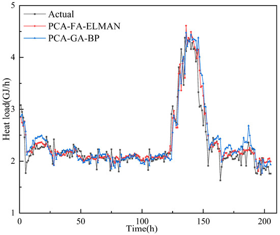 Figure 10. Comparison between the actual data of heat load and results of a one-hour-ahead heat load prediction using the PCA-GA-BP and PCA-FA-ELMAN methods.
5. Conclusions
PCA-BP-ELMAN, FA-ELMAN, and GA-BP are established to apply heat load prediction. This study aimed to compare the prediction accuracy of these three combined models. The main conclusions are as follows:
- (1)
- To assess the prediction performance of six commonly used individual models, we selected eight initial characteristics: water supply temperature, return water temperature, circulation flow, solar radiation, heat load, outdoor temperature, wind speed, and relative humidity at time t-1. The results indicated that the BP and ELMAN neural network prediction models had a MAPE of less than 10% and an MSE of less than 0.1 GJ2/h2. Furthermore, the RMSE and MAE were both less than 0.3 GJ/h and 0.2 GJ/h, respectively, suggesting that these models demonstrate high prediction accuracy.
- (2)
- The dimensionality of the characteristic variables that impact heating load is reduced from 8 to 4 using PCA, and the input parameters of the neural network are optimized accordingly. In predicting heat load, the most significant principal components are return water temperature, circulation flow, historical heat load, and outdoor temperature. Following these are relative humidity, solar radiation, water supply temperature, and wind speed.
- (3)
- The application of PCA-minSSE, FA, and GA algorithms in heat load prediction has been shown to improve the accuracy of the prediction model. The models with the highest prediction performance, ranked from high to low, are FA-ELMAN, PCA-BP-ELMAN, and GA-BP. When compared to individual neural network models with superior prediction performance, the combined model exhibits a decrease in MAPE of 2.25%.
Author Contributions
Conceptualization, W.A., X.Z. and J.L.; methodology, J.L., M.K.K. and K.Y.; software, W.A.; validation, W.A. and J.L.; formal analysis, W.A.; investigation, W.A., K.Y., M.K.K. and J.L.; resources, J.L.; data curation, W.A. and J.L.; writing—original draft preparation, W.A., X.Z., M.K.K. and J.L.; writing—review and editing, W.A., X.Z., K.Y., M.K.K. and J.L.; visualization, W.A.; supervision, J.L., M.K.K. and K.Y.; project administration, J.L.; funding acquisition, J.L. All authors have read and agreed to the published version of the manuscript.
Funding
This work was funded by the Natural Science Foundation of Shandong Province (ZR2021ME199, ZR2020ME211 and ZR2021ME237) and the Support Plan for Outstanding Youth Innovation Team in Colleges and Universities of Shandong Province (2019KJG005).
Data Availability Statement
Not applicable.
Acknowledgments
This work was also supported by the Plan of Introduction and Cultivation for Young Innovative Talents in Colleges and Universities of Shandong Province.
Conflicts of Interest
The authors declare no conflict of interest.
Nomenclature
| bj | information contribution rate of principal component Fj |
| dij | the distance between any two fireflies i and j |
| et | the prediction error of the combined prediction model at time t |
| eit | the prediction error of the ith individual model at time t |
| fi | the fitness of individual Xi |
| F | the fitness of individual |
| Fm | the mth principal component |
| F(t − 1) | circulation flow at time t-1, m3/h |
| H | let H = [1KK1]T |
| H(t) | relative humidity at time t, % |
| I0 | the maximum brightness of fireflies |
| J | the sum of squares of combined prediction errors |
| li | the weight coefficient |
| m | the number of influence factors |
| n | the number of influence factor samples |
| N | the number of population individuals |
| P | the selection probability |
| Q(t − 1) | heat load at time t-1, GJ/h |
| rij | the correlation coefficient |
| R | the correlation coefficient matrix |
| sj | the sample standard deviation of the jth influence factor |
| S(t − 1) | solar radiation at t-1 time, W/m2 |
| T(t) | outside temperature at time t, °C |
| TR(t − 1) | return water temperature at time t-1, °C |
| TS(t − 1) | water supply temperature at time t-1, °C |
| uj | the eigenvector |
| wi | the pattern of movement for the reference firefly i |
| wi, k | the coordinates of the ith firefly on the k dimension |
| wj, k | the coordinates of the jth firefly on the k dimension |
| Wt | wind speed at time t, m/s |
| the mean of the simulated values | |
| xi | the ith simulated value |
| the sample mean of the jth influence factor | |
| xt | the actual value of the heat load at time t |
| the combined predicted value of heat load at time t | |
| xij | the ith index of the jth influence factor |
| xit | the heat load prediction of the ith model at time t |
| a standardized indicator | |
| the kth standardized index of the ith influence factor | |
| the kth standardized index of the jth influence factor | |
| the mean value of the measured value | |
| yi | the ith actual measured value |
| Abbreviation | |
| Bi-LSTM | bidirectional long short-term memory |
| BP | back propagation |
| CNN | convolutional neural network |
| FA | firefly algorithm |
| GA | genetic algorithm |
| LSTM | long short-term memory |
| minSSE | the minimum sum of squares of the combined prediction errors |
| MAE | Mean Absolute Error, GJ/h |
| MAPE | Mean Absolute Percentage Error, % |
| MSE | Mean Square Error, GJ2/h2 |
| PCA | principal component analysis |
| RF | Random Forest |
| RMSE | Root Mean Square Error, GJ/h |
| RNNs | recurrent neural networks |
| SVR | support rector regression |
| Greek Symbols | |
| α | the step factor |
| αp | the cumulative contribution rate |
| β0 | the attraction of fireflies at the light source |
| β(d) | the attractiveness function |
| γ | the absorption coefficient of light intensity |
| εi | the vector of random numbers |
| λj | the eigenvalues |
| Subscripts | |
| i | represents the ith |
| j | represents the jth |
| k | represents the kth |
| t | time |
References
- Zhang, Y.; Xia, J.; Fang, H.; Jiang, Y.; Liang, Z. Field tests on the operational energy consumption of Chinese district heating systems and evaluation of typical associated problems. Energy Build. 2020, 224, 110269. [Google Scholar] [CrossRef]
- Eguía, P.; Granada, E.; Alonso, J.M.; Arce, E.; Saavedra, A. Weather datasets generated using kriging techniques to calibrate building thermal simulations with TRNSYS. J. Build. Eng. 2016, 7, 78–91. [Google Scholar] [CrossRef]
- Yu, S.; Cui, Y.; Xu, X.; Feng, G. Impact of Civil Envelope on Energy Consumption based on EnergyPlus. Procedia Eng. 2015, 121, 1528–1534. [Google Scholar] [CrossRef]
- Amasyali, K.; El-Gohary, N.M. A review of data-driven building energy consumption prediction studies. Renew. Sustain. Energy Rev. 2018, 81, 1192–1205. [Google Scholar] [CrossRef]
- Mat Daut, M.A.; Hassan, M.Y.; Abdullah, H.; Rahman, H.A.; Abdullah, M.P.; Hussin, F. Building electrical energy consumption forecasting analysis using conventional and artificial intelligence methods: A review. Renew. Sustain. Energy Rev. 2017, 70, 1108–1118. [Google Scholar] [CrossRef]
- Park, B.R.; Choi, E.J.; Hong, J.; Lee, J.H.; Moon, J.W. Development of an energy cost prediction model for a VRF heating system. Appl. Therm. Eng. 2018, 140, 476–486. [Google Scholar] [CrossRef]
- Fan, C.; Ding, Y. Cooling load prediction and optimal operation of HVAC systems using a multiple nonlinear regression model. Energy Build. 2019, 197, 7–17. [Google Scholar] [CrossRef]
- Su, M.; Liu, J.; Zhou, S.; Miao, J.; Kim, M.K. Dynamic prediction of the pre-dehumidification of a radiant floor cooling and displacement ventilation system based on computational fluid dynamics and a back-propagation neural network: A case study of an office room. Indoor Built Environ. 2022, 31, 2386–2410. [Google Scholar] [CrossRef]
- Ren, L.; An, F.; Su, M.; Liu, J. Exposure Assessment of Traffic-Related Air Pollution Based on CFD and BP Neural Network and Artificial Intelligence Prediction of Optimal Route in an Urban Area. Buildings 2022, 12, 1227. [Google Scholar] [CrossRef]
- Kim, M.K.; Cremers, B.; Liu, J.; Zhang, J.; Wang, J. Prediction and correlation analysis of ventilation performance in a residential building using artificial neural network models based on data-driven analysis. Sustain. Cities Soc. 2022, 83, 103981. [Google Scholar] [CrossRef]
- Su, M.; Liu, J.; Kim, M.K.; Wu, X. Predicting moisture condensation risk on the radiant cooling floor of an office using integration of a genetic algorithm-back-propagation neural network with sensitivity analysis. Energy Built Environ. 2024, 5, 110–129. [Google Scholar] [CrossRef]
- Liu, J.; Yin, Y. Power Load Forecasting Considering Climate Factors Based on IPSO-Elman Method in China. Energies 2022, 15, 1236. [Google Scholar] [CrossRef]
- Moayedi, H.; Mosavi, A. Suggesting a Stochastic Fractal Search Paradigm in Combination with Artificial Neural Network for Early Prediction of Cooling Load in Residential Buildings. Energies 2021, 14, 1649. [Google Scholar] [CrossRef]
- Yousaf, A.; Asif, R.M.; Shakir, M.; Rehman, A.U.; Adrees, M.S. An Improved Residential Electricity Load Forecasting Using a Machine-Learning-Based Feature Selection Approach and a Proposed Integration Strategy. Sustainability 2021, 13, 6199. [Google Scholar] [CrossRef]
- Wei, Y.; Xia, L.; Pan, S.; Wu, J.; Zhang, X.; Han, M.; Zhang, W.; Xie, J.; Li, Q. Prediction of occupancy level and energy consumption in office building using blind system identification and neural networks. Appl. Energy 2019, 240, 276–294. [Google Scholar] [CrossRef]
- Zhao, H.X.; Magoules, F. Parallel Support Vector Machines Applied to the Prediction of Multiple Buildings Energy Consumption. J. Algorithms Comput. Technol. 2010, 4, 231–250. [Google Scholar] [CrossRef]
- Guo, Y.; Wang, J.; Chen, H.; Li, G.; Liu, J.; Xu, C.; Huang, R.; Huang, Y. Machine learning-based thermal response time ahead energy demand prediction for building heating systems. Appl. Energy 2018, 221, 16–27. [Google Scholar] [CrossRef]
- Fan, C.; Xiao, F.; Wang, S. Development of prediction models for next-day building energy consumption and peak power demand using data mining techniques. Appl. Energy 2014, 127, 1–10. [Google Scholar] [CrossRef]
- Chou, J.-S.; Bui, D.-K. Modeling heating and cooling loads by artificial intelligence for energy-efficient building design. Energy Build. 2014, 82, 437–446. [Google Scholar] [CrossRef]
- Park, T.C.; Kim, U.S.; Kim, L.-H.; Jo, B.W.; Yeo, Y.K. Heat consumption forecasting using partial least squares, artificial neural network and support vector regression techniques in district heating systems. Korean J. Chem. Eng. 2010, 27, 1063–1071. [Google Scholar] [CrossRef]
- Meng, Q.; Xi, Y.; Ren, X.; Li, H.; Jiang, L.; Yang, L. Thermal Energy Storage Air-conditioning Demand Response Control Using Elman Neural Network Prediction Model. Sustain. Cities Soc. 2022, 76, 103480. [Google Scholar] [CrossRef]
- Wang, Z.; Hong, T.; Piette, M.A. Building thermal load prediction through shallow machine learning and deep learning. Appl. Energy 2020, 263, 114683. [Google Scholar] [CrossRef]
- Bourdeau, M.; Zhai, X.; Nefzaoui, E.; Guo, X.; Chatellier, P. Modeling and forecasting building energy consumption: A review of data-driven techniques. Sustain. Cities Soc. 2019, 48, 101533. [Google Scholar] [CrossRef]
- Yu, W.; Li, B.; Jia, H.; Zhang, M.; Wang, D. Application of multi-objective genetic algorithm to optimize energy efficiency and thermal comfort in building design. Energy Build. 2015, 88, 135–143. [Google Scholar] [CrossRef]
- Song, J.; Zhang, L.; Xue, G.; Ma, Y.; Gao, S.; Jiang, Q. Predicting hourly heating load in a district heating system based on a hybrid CNN-LSTM model. Energy Build. 2021, 243, 110998. [Google Scholar] [CrossRef]
- Qi, L.; Feng, Z. Improved BP Neural Network of Heat Load Forecasting Based on Temperature and Date Type. J. Syst. Simul. 2018, 30, 1464–1472. [Google Scholar] [CrossRef]
- Ding, Y.; Zhang, Q.; Yuan, T.; Yang, K. Model input selection for building heating load prediction: A case study for an office building in Tianjin. Energy Build. 2018, 159, 254–270. [Google Scholar] [CrossRef]
- Zhao, A.; Mi, L.; Xue, X.; Xi, J.; Jiao, Y. Heating load prediction of residential district using hybrid model based on CNN. Energy Build. 2022, 266, 112122. [Google Scholar] [CrossRef]
- Al-Shammari, E.T.; Keivani, A.; Shamshirband, S.; Mostafaeipour, A.; Yee, P.L.; Petković, D.; Ch, S. Prediction of heat load in district heating systems by Support Vector Machine with Firefly searching algorithm. Energy 2016, 95, 266–273. [Google Scholar] [CrossRef]
- Kapalo, P.; Adamski, M. The Analysis of Heat Consumption in the Selected City. Lect. Notes Civ. Eng. 2021, 100, 158–165. [Google Scholar] [CrossRef]
- Yang, M. Numerical study of the heat transfer to carbon dioxide in horizontal helically coiled tubes under supercritical pressure. Appl. Therm. Eng. 2016, 109, 685–696. [Google Scholar] [CrossRef]
- Lam, J.C.; Wan, K.K.W.; Wong, S.L.; Lam, T.N.T. Principal component analysis and long-term building energy simulation correlation. Energy Convers. Manag. 2010, 51, 135–139. [Google Scholar] [CrossRef]
- Tang, D.; Zhang, Z.; Hua, L.; Pan, J.; Xiao, Y. Prediction of cold start emissions for hybrid electric vehicles based on genetic algorithms and neural networks. J. Clean. Prod. 2023, 420, 138403. [Google Scholar] [CrossRef]
- Protić, M.; Shamshirband, S.; Petković, D.; Abbasi, A.; Mat Kiah, M.L.; Unar, J.A.; Živković, L.; Raos, M. Forecasting of consumers heat load in district heating systems using the support vector machine with a discrete wavelet transform algorithm. Energy 2015, 87, 343–351. [Google Scholar] [CrossRef]
- Paudel, S.; Elmitri, M.; Couturier, S.; Nguyen, P.H.; Kamphuis, R.; Lacarriere, B.; Le Corre, O. A relevant data selection method for energy consumption prediction of low energy building based on support vector machine. Energy Build. 2017, 138, 240–256. [Google Scholar] [CrossRef]
- Li, Q.; Meng, Q.; Cai, J.; Yoshino, H.; Mochida, A. Predicting hourly cooling load in the building: A comparison of support vector machine and different artificial neural networks. Energy Convers. Manag. 2009, 50, 90–96. [Google Scholar] [CrossRef]
- Cai, C.; Qian, Q.; Fu, Y. Application of BAS-Elman Neural Network in Prediction of Blasting Vibration Velocity. Procedia Comput. Sci. 2020, 166, 491–495. [Google Scholar] [CrossRef]
- Wang, Y.; Zhan, C.; Li, G.; Zhang, D.; Han, X. Physics-guided LSTM model for heat load prediction of buildings. Energy Build. 2023, 294, 113169. [Google Scholar] [CrossRef]
- Xue, G.; Qi, C.; Li, H.; Kong, X.; Song, J. Heating load prediction based on attention long short term memory: A case study of Xingtai. Energy 2020, 203, 117846. [Google Scholar] [CrossRef]
- Li, J.; Zhu, D.; Li, C. Comparative analysis of BPNN, SVR, LSTM, Random Forest, and LSTM-SVR for conditional simulation of non-Gaussian measured fluctuating wind pressures. Mech. Syst. Signal Process. 2022, 178, 109285. [Google Scholar] [CrossRef]
- Lin, K.; Zhao, Y.; Tian, L.; Zhao, C.; Zhang, M.; Zhou, T. Estimation of municipal solid waste amount based on one-dimension convolutional neural network and long short-term memory with attention mechanism model: A case study of Shanghai. Sci. Total Environ. 2021, 791, 148088. [Google Scholar] [CrossRef] [PubMed]
- Cui, M. District heating load prediction algorithm based on bidirectional long short-term memory network model. Energy 2022, 254, 124283. [Google Scholar] [CrossRef]
- Yan, Q.; Lu, Z.; Liu, H.; He, X.; Zhang, X.; Guo, J. An improved feature-time Transformer encoder-Bi-LSTM for short-term forecasting of user-level integrated energy loads. Energy Build. 2023, 297, 113396. [Google Scholar] [CrossRef]
- Yang, Y.; Zheng, X.; Sun, Z. Coal Resource Security Assessment in China: A Study Using Entropy-Weight-Based TOPSIS and BP Neural Network. Sustainability 2020, 12, 2294. [Google Scholar] [CrossRef]
- Xie, L. The Heat load Prediction Model based on BP Neural Network-markov Model. Procedia Comput. Sci. 2017, 107, 296–300. [Google Scholar] [CrossRef]
- Lu, C.; Li, S.; Lu, Z. Building energy prediction using artificial neural networks: A literature survey. Energy Build. 2022, 262, 111718. [Google Scholar] [CrossRef]
- Chaki, S.; Biswas, T.K. An ANN-entropy-FA model for prediction and optimization of biodiesel-based engine performance. Appl. Soft Comput. 2023, 133, 109929. [Google Scholar] [CrossRef]
- Ding, C.; Xia, Y.; Yuan, Z.; Yang, H.; Fu, J.; Chen, Z. Performance prediction for a fuel cell air compressor based on the combination of backpropagation neural network optimized by genetic algorithm (GA-BP) and support vector machine (SVM) algorithms. Therm. Sci. Eng. Prog. 2023, 44, 102070. [Google Scholar] [CrossRef]
- Ling, J.; Dai, N.; Xing, J.; Tong, H. An improved input variable selection method of the data-driven model for building heating load prediction. J. Build. Eng. 2021, 44, 103255. [Google Scholar] [CrossRef]
- Wei, Z.; Zhang, T.; Yue, B.; Ding, Y.; Xiao, R.; Wang, R.; Zhai, X. Prediction of residential district heating load based on machine learning: A case study. Energy 2021, 231, 120950. [Google Scholar] [CrossRef]
- Fu, X.; Huang, S.; Li, R.; Guo, Q. Thermal Load Prediction Considering Solar Radiation and Weather. Energy Procedia 2016, 103, 3–8. [Google Scholar] [CrossRef]
- Sun, J.; Gong, M.; Zhao, Y.; Han, C.; Jing, L.; Yang, P. A hybrid deep reinforcement learning ensemble optimization model for heat load energy-saving prediction. J. Build. Eng. 2022, 58, 105031. [Google Scholar] [CrossRef]
Disclaimer/Publisher’s Note: The statements, opinions and data contained in all publications are solely those of the individual author(s) and contributor(s) and not of MDPI and/or the editor(s). MDPI and/or the editor(s) disclaim responsibility for any injury to people or property resulting from any ideas, methods, instructions or products referred to in the content. |
© 2023 by the authors. Licensee MDPI, Basel, Switzerland. This article is an open access article distributed under the terms and conditions of the Creative Commons Attribution (CC BY) license (https://creativecommons.org/licenses/by/4.0/).