Article

Improved Data-Driven Building Daily Energy Consumption Prediction Models Based on Balance Point Temperature

1
School of Architecture, Huaqiao University, Xiamen 361021, China
2
Xiamen Key Laboratory of Ecological Building Construction, Xiamen 361021, China
3
Faculty of Forestry, University of British Columbia, Vancouver, BC V6T 1Z4, Canada
*
Authors to whom correspondence should be addressed.
Buildings 2023, 13(6), 1423; https://doi.org/10.3390/buildings13061423
Submission received: 9 May 2023 / Revised: 24 May 2023 / Accepted: 29 May 2023 / Published: 31 May 2023
(This article belongs to the Special Issue AI and Data Analytics for Energy-Efficient and Healthy Buildings)

Abstract

:
The data-driven models have been widely used in building energy analysis due to their outstanding performance. The input variables of the data-driven models are crucial for their predictive performance. Therefore, it is meaningful to explore the input variables that can improve the predictive performance, especially in the context of the global energy crisis. In this study, an algorithm for calculating the balance point temperature was proposed for an apartment community in Xiamen, China. It was found that the balance point temperature label (BPT label) can significantly improve the daily energy consumption prediction accuracy of five data-driven models (BPNN, SVR, RF, LASSO, and KNN). Feature importance analysis showed that the importance of the BPT label accounts for 25%. Among all input variables, the daily minimum temperature is the decisive factor that affects energy consumption, while the daily maximum temperature has little impact. In addition, this study also provides recommendations for selecting these model tools under different data conditions: when the input variable data is insufficient, KNN has the best predictive performance, while BPNN is the best model when the input data is sufficient.

1. Introduction

As global warming and energy crisis intensify, the international community is increasingly focused on sustainable development. As one of the main sources of global energy consumption, the energy efficiency and emissions of the construction industry are becoming increasingly important [1,2]. Energy consumption analysis and prediction of buildings are of great significance for improving building energy efficiency, reducing energy waste and emissions, and promoting the implementation of the double carbon strategy [3]. Through scientific analysis and accurate prediction of building energy consumption, it can provide strong support for decision-making in building design, operation, and management.
Currently, there are many methods for predicting building energy consumption, which can be classified into two categories based on the analysis methods: simulation technology based on physical principles and data-driven methods based on artificial intelligence algorithms.
The simulation method is based on thermodynamics to establish a physical model for evaluating building energy consumption. Currently, there are various software tools for simulating building energy consumption, such as DOE-2 [4], Energy Plus [5] TRNSYS [6], Design Builder [7], etc.
Compared with simulation methods, data-driven methods based on artificial intelligence algorithms are commonly used for building energy consumption prediction.
The data-driven approach uses mathematical analysis methods to establish mathematical models of energy consumption systems based on known input and output data. Data-driven models applied in the field of building energy consumption prediction include Multiple Linear Regression (MLR) [8], Back Propagation Neural Network (BPNN) [9], Support Vector Regression (SVR) [10], Random Forest (RF) [11], K-Nearest Neighbors (KNN) regression [12], and Least Absolute Shrinkage and Selection Operator (LSAAO) [13] regression. These models can identify potential (sometimes previously unknown) relationships between input and output variables through mathematical analysis. These AI-based data-driven algorithms can achieve high prediction accuracy without requiring much knowledge of building thermodynamics.
With the continuous development of computer science algorithms, data-driven models have been widely used in the field of building energy analysis due to their excellent performance. The input variables of data-driven models are crucial, and the effectiveness of variables directly affects the predictive performance of the model. Therefore, in order to increase the predictive accuracy of data-driven models, researchers have to look for more input variables [9]. However, not all variables that affect the model can be effectively obtained, and some variables are difficult to measure in practical applications. Therefore, mining input variables that can significantly increase the predictive accuracy of the model is a problem that researchers need to explore in depth.
The following researchers use data-driven modeling methods in energy forecasting research tasks.
Javed F et al. [14] used an ANN model with input feature variables including outdoor temperature, time, number of individuals, type of enclosure structure, and household appliance load to predict the expected daily electricity load. Li Q et al. [15] used the DeST simulation software to predict the cooling energy consumption of buildings with the SVR model, taking outdoor dry bulb temperature, relative humidity, and solar radiation as input variables. Sholahudin et al. [16] used dynamic ANN to predict the hourly thermal load of buildings with dry bulb temperature, relative humidity, solar radiation, and wind degree as input variables. Y. Ding et al. [17] used meteorological information and historical data as feature variables to predict the cooling energy consumption of commercial buildings using SVR. Furthermore, it used Historical Meteorological data as feature vectors and used MLR and SVR to predict the heating energy consumption of commercial buildings [18]. Cheng Fan et al. [19] conducted building energy consumption prediction tasks using various data-driven models with input variables including outdoor temperature, outdoor relative humidity, chilled water supply temperature, chilled water return temperature, and chilled water flow rate. Antonio B et al. [20] utilized MLR and SVR to predict building energy consumption using Meteorological information and time index as input variables. Gorazd K et al. [21] noticed the impact of the balance point temperature on energy consumption and therefore used heating degree days to predict instantaneous energy consumption. A simplified model of heat load prediction, which combines the quasi-steady-state thermal balance calculation procedure in ISO 52016 and the variable-base degree-days method, was proposed by Z Hao et al. [22]. However, there was no calculation of the balance point temperature involved in specific cases. Aranda et al. [23] established three different MLR models to assess the energy performance of bank buildings in Spain using building characteristics and climate areas.
Based on the above discussion, we have found the following issues in the existing research on building energy consumption prediction that have not been well addressed.
  • The balance point temperature is one of the factors that affect building energy consumption. How to use statistical methods to identify the balance point temperature scientifically and effectively?
  • Currently, research on using balance point temperature as an input variable in data-driven models is relatively scarce. Can the addition of a balance point temperature label (BPT label) improve the prediction accuracy of data-driven models?
  • Is there a difference in prediction accuracy of different data-driven model tools trained on the same dataset, and which data-driven model tool should be prioritized under different data conditions?
  • What is the importance of each input variable, including the BPT label, in the prediction model?
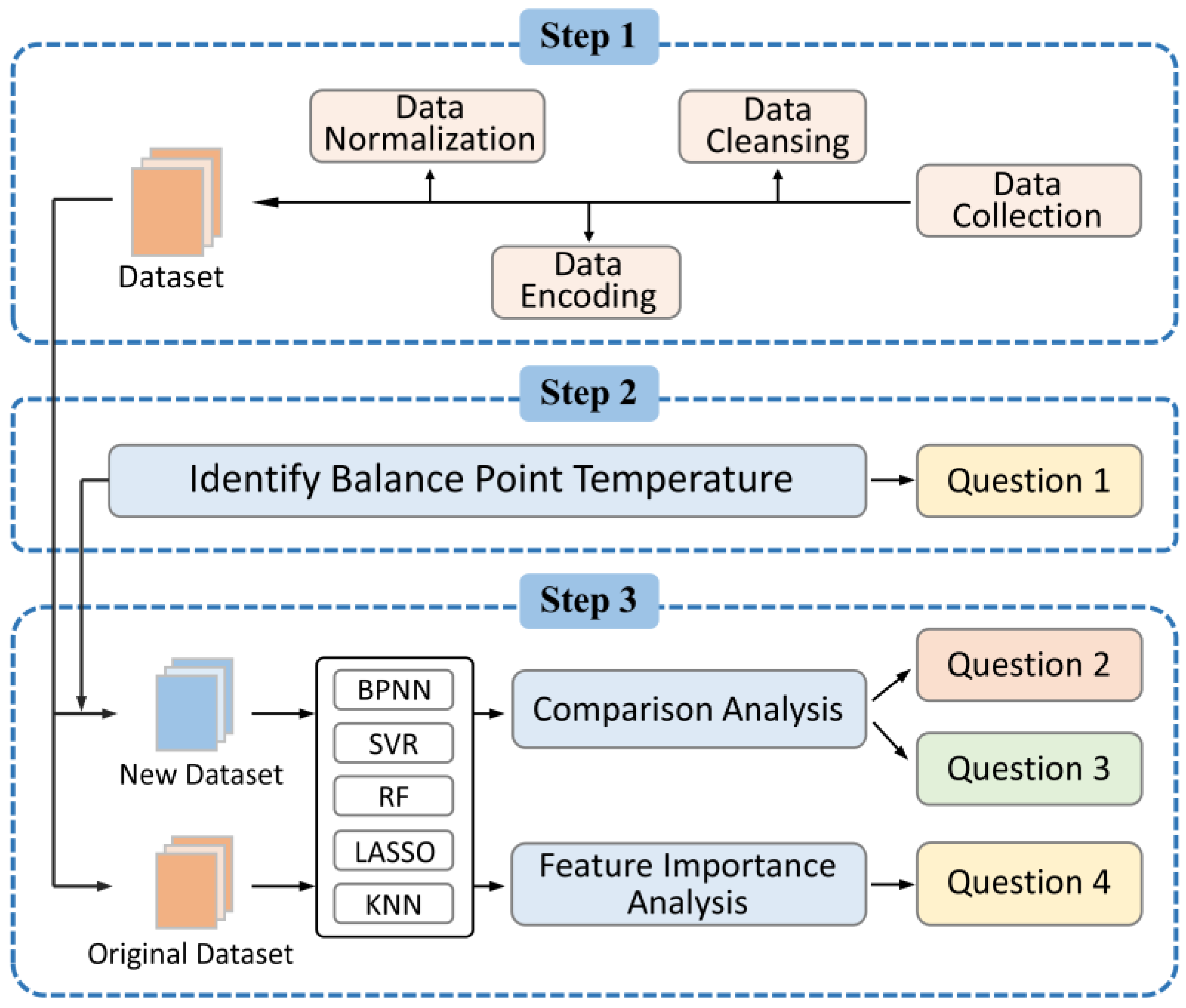
This study takes an apartment community in Xiamen, China as an example and uses different data-driven models to predict and analyze the daily energy consumption of the building, and answers the above questions. Statistical methods are used in this article to effectively identify the balance point temperature of apartment buildings and analyze the impact of balance point temperature labels on the predictive performance of data-driven models. Specifically, this study considers five representative data-driven models (BPNN, SVR, RF, LASSO, and KNN) and studies the differences in the predictive performance of various data-driven models.
The rest of the paper is organized as follows: Section 2 presents the research outline, data preprocessing, specific algorithms for each data-driven model, and performance evaluation indicators for the models. Section 3 is a case study that includes analysis methods for identifying the balance point temperature, detailed data, and model implementation details. Section 4 is the analysis and discussion, which compares the performance of various data-driven models using model performance evaluation indicators and analyzes the importance of input variables. The conclusion is drawn in Section 5.

2. Methodology

This section introduces the research structure and framework of this article, as shown in Figure 1, which includes three steps. The first step is data collection, data cleaning, data encoding, and data normalization, to obtain a dataset suitable for the research of this research. The second step is the identification of the balance point temperature, which answers the first question proposed in the introduction of this study. A new dataset is formed by adding the BPT label to the original dataset. In the third part, five data-driven models are used to analyze building energy consumption prediction for both new and old datasets, and the prediction accuracy is compared and analyzed. Feature importance analysis is also conducted for input variables. These, respectively, answer the second to fourth questions proposed in the introduction.

2.1. Data Collection

The data collected in this study is related to an apartment complex located in Xiamen, China, shown in Figure 2.
The apartment building was constructed and put into use in 2014. It is an outdoor corridor-style building with a frame structure, consisting of 9 floors and rooms with a usable area of 25.33 m2. All electrical appliances in the rooms are uniformly purchased by the building developer, which means that the models, specifications, power, and other parameters of the electrical appliances in each room are consistent. Each room is equipped with two LED tubes, a fan, an air conditioner, and four sockets. Table 1 summarizes the details. The apartment provides an independent hot water system, which does not consume electricity when using hot water.
This study used explanatory variable and dependent variable data from 1 September 2020 to 1 September 2021, spanning a full year. This section describes the methods and details of how these variables were collected.

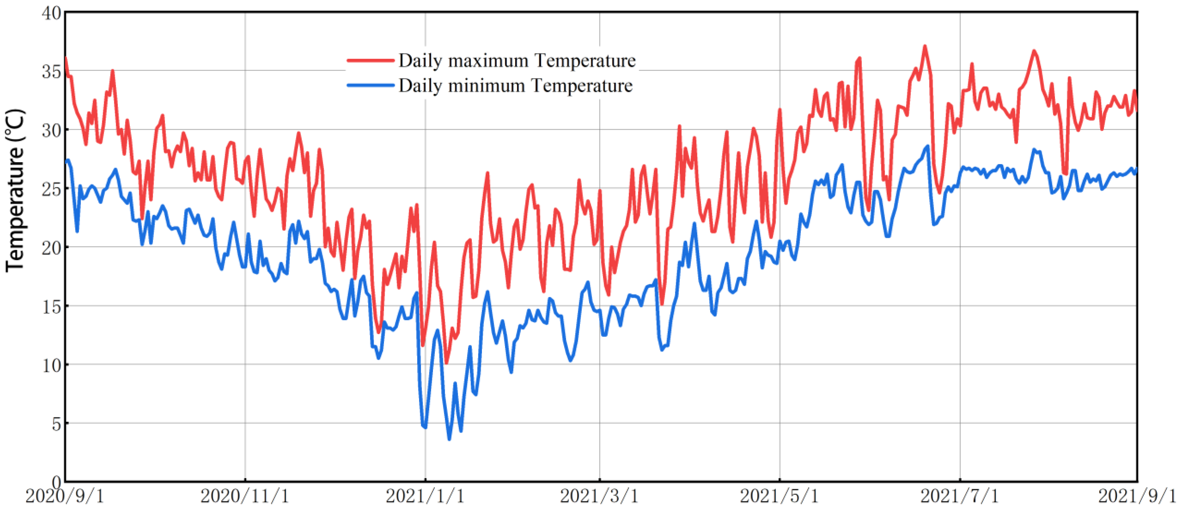
2.1.1. Electricity Consumption Data

The dependent variable, the energy consumption of the building, is obtained from the central intelligent electricity meters. The electricity consumption data for each room is obtained from the central intelligent meter with a time step size of day-by-day. It includes the total electricity consumption of the room, including air conditioning and lighting. Since the room type and the number of users are the same, the room’s daily average electricity consumption is selected as the dependent variable, which is the total building energy consumption divided by the number of rooms (after data cleaning, details see Section 2.2.1).

2.1.2. Weather Data

In this study, three weather variables, including the daily minimum temperature, daily maximum temperature, and precipitation, were used in the Xiamen area. These climate data were obtained from the China Meteorological Data Service Center [24]. Figure 3 shows the variation in air temperature between 1 September 2020 and 1 September 2021. It is worth noting that the precipitation fluctuates greatly, with a value of 0 when there is no rain, and several hundred when it rains. Therefore, this study sets the explanatory variable of precipitation as a categorical variable, namely the sunny-rainy day index, which will be explained in the following text.

2.1.3. Sunny Day Index

The sunshine-rainy index [9] is a categorical type of climate parameter. Rainy days may reduce the desire for outdoor activities, thus increasing the use of indoor facilities. Therefore, whether it is raining or not is used as an explanatory variable in the energy consumption prediction model. This study defines rainy days as those with a total daily precipitation of more than 5 mm between 6:00 a.m. and 11:00 p.m. The virtual value of rainy days is 1, while the virtual value of non-rainy days is 0.

2.1.4. Holiday Index

Building occupancy rate significantly affects its energy demand. However, it is difficult to accurately measure the actual building occupancy rate in actual research, therefore this study introduced a categorical variable “holiday index” to describe the occupancy rate of the buildings. The occupancy rate of holidays will be greater than that of working days. The virtual value for holidays is 1 and for working days is 0. The specific dates for the holidays are obtained from the government website [25].
In summary, the dependent and explanatory variables used in this article are shown in Table 2. It is worth noting that, since the building area, orientation, and indoor electrical equipment (including air conditioning) parameters of these eight buildings are the same, this study did not consider these parameters as explanatory variables.

2.2. Data Preparation

2.2.1. Data Cleansing

During the process of data collection, data loss, and anomalies often occur due to equipment malfunctions or weather conditions. Therefore, it is necessary to clean the data, which is a crucial step before analysis and research [26].
The main purpose of data cleaning in this study is to eliminate the adverse effects of missing value, vacant, and anomalous data rooms, and remove them from the dataset. A room is defined as a missing value room if it has no electricity consumption data for at least three days, but rooms with less than three missing values can be repaired using linear interpolation techniques. A vacant room is defined as one where the daily electricity consumption in a room is zero or below 0.1 kWh hours for five consecutive days. A room is considered an anomalous data room if its electricity consumption remains the same for five consecutive days and is not equal to zero.
After data cleaning, a total of 95 rooms were deleted. The electricity consumption data of 427 rooms were analyzed.

2.2.2. Data Encoding and Normalization

Before performing prediction tasks using data-driven models, categorical features need to be encoded into 0 or 1 [27], such as the holiday index and the sunny day index mentioned in the following text. Data normalization is an important step in data analysis. It scales the datasets of different input variables to the interval [0,1] to eliminate the weakening of analysis caused by different scales and dimensions of datasets. In this study, the Z-score standardization [28] method is selected, as shown in Equation (1).
x ^ i = x i x δ
In Equation (1), x i is the i-th value, x is the average of the variable, δ is the standard deviation, and x ^ i is the normalized value.

2.3. Data-Driven Models

2.3.1. Backpropagation Neural Network

The Backpropagation Neural Network (BPNN) [29] is a training algorithm for artificial neural networks. It uses the backpropagation algorithm to adjust the weights and thresholds in the neural network so that the network can fit the training data with minimum error. The BPNN consists of an input layer, a hidden layer, and an output layer, and is commonly used for classification and regression tasks. During the training process, the BPNN calculates the error and adjusts the weights and thresholds through the backpropagation algorithm, in order to fit the training data as accurately as possible.

2.3.2. Random Forest

Random Forest (RF) algorithms [30,31] can be summarized in the following steps:
  • Select n samples from the dataset using a bootstrapped sampling approach to form a training set;
  • Generate a decision tree using the sampled dataset.
  • Repeat steps 1 to 2 for k times, where k is the number of trees in the RF.
  • Use the trained Random Forest to predict the test samples and decide the prediction result using the voting method, as shown in Figure 3.
The two common Variable Importance Measure (VIM) [32,33] calculation methods for RF are the Gini index and Out-of-Bag (OOB) error rate. This paper uses the OOB error rate to analyze the VIM. The higher the average of the decrease of OOB error rate, the higher the VIM; otherwise, the lower the VIM.
The M target variables are calculated according to Equation (2) and their importance is sorted based on their VIM values, as follows:
  • Construct N decision trees;
  • When the current decision tree ktree = 1, the obtain the corresponding OOB data OOB k ;
  • Calculate the prediction error eerOOB k of the current tree for OOB k ;
  • Randomly perturb the i-th feature of OOB k as OOB k i , calculate the prediction error eerOOB k i of the current tree for OOB k i ;
  • For each decision tree, ktree = 2, …, N, repeat steps 2–4;
  • Calculate the VIM of the target feature according to Equation (2).
VIM = 1 N k = 1 N ( eerOOB k i eerOOB k )
In the formula, N is the number of trees, eerOOB k i and eerOOB k represent the prediction errors of the OOB data with and without perturbation for the i-th feature under the ktree-th tree case, respectively.

2.3.3. Support Vector Regression

Support Vector Regression(SVR) [34] is the application of a Support Vector Machine (SVM) in regression problems. Unlike traditional regression algorithms such as linear regression and polynomial regression, the goal of SVR is to find one or more curves that minimize the error between these curves and the training data, while also avoiding overfitting as much as possible. The core idea of SVR is to introduce kernel functions, map the original data to a high-dimensional space, and find the optimal hyperplane to achieve classification or regression. In regression problems, the goal of SVR is to find a hyperplane that minimizes the distance between all training samples and the hyperplane, while also satisfying a certain tolerance, which allows for a certain degree of error. The advantages of SVR are that it can handle nonlinear problems and has good generalization ability. It can also improve the fitting ability of the model by using kernel functions for nonlinear data mapping.

2.3.4. Least Absolute Shrinkage and Selection Operator

Least Absolute Shrinkage and Selection Operator (LASSO) [35], is a machine learning algorithm used for feature selection and regression analysis. LASSO is a linear regression algorithm that limits the complexity of the model and the number of features by adding an L1 regularization term to the loss function. It involves adding a penalty term to the standard least squares regression objective, which helps to reduce the magnitude of the coefficients of the features in the model. The penalty term is based on the absolute value of the coefficients and the algorithm tries to minimize the sum of the residuals and the penalty term. LASSO is particularly useful when dealing with high-dimensional datasets where there are many features but only a small number of them are relevant for the prediction task.

2.3.5. K-Nearest Neighbors

K-Nearest Neighbors (KNN) [36] is a basic supervised learning algorithm that is applied in both classification and regression tasks. It is a non-parametric algorithm, which means that it does not make any assumptions about the data and directly learns the model from the data. The basic idea of the KNN algorithm is to find the k nearest known samples with class labels to a new sample, and then predict or classify based on the class labels of these k samples. In classification tasks, the KNN algorithm classifies the new sample as the class that appears most frequently among the k nearest neighbors. In regression tasks, the KNN algorithm sets the predicted value of the new sample as the average value of the k nearest neighbors. This article belongs to the regression task.

2.4. Model Performance Evaluation Metrics

In order to assess the predictive performance of the models, three metrics [37] commonly used in electricity load forecasting are used in this study, namely, coefficient of variation-root mean square error (CV−RMSE), normalized mean bias error (NMBE) and regression determination coefficient (R2). The calculation of the above indicators is shown in Formulas (3) to (5). In the formulas, y ^ i is the prediction value, y i is the actual value and y ¯ is the average of the actual values.
CV RMSE = i = 1 n ( y i y ^ i ) 2 n y ¯ × 100 %
NMBE = i = 1 n ( y i y ^ i ) n × y ¯ × 100 %
R 2 = 1 i = 1 n ( y i y ^ i ) 2 i = 1 n ( y i y ¯ i ) 2

3. Case Study

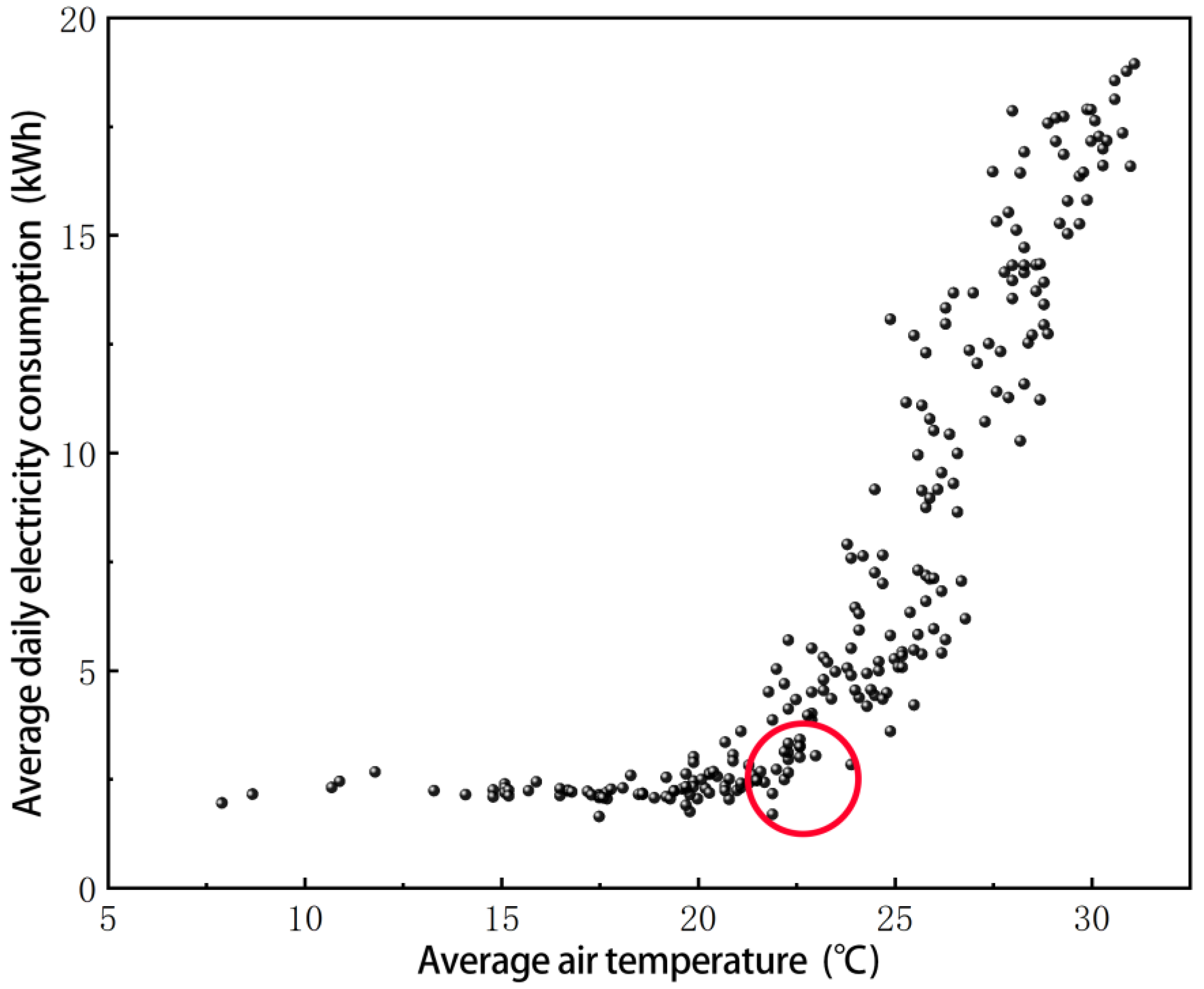
3.1. Identifying the Balance Point Temperature

Xiamen is located in the hot summer and warm winter region of China and is a city primarily focused on cooling in the summer months with a short period of heating required in the winter. Additionally, for energy-saving purposes, the air conditioning units installed by apartment complexes do not have a cooling function. As shown in the scatter diagram in Figure 4, the energy consumption of a building is highly correlated with the outdoor air temperature, especially during the warmer phases when the air temperature influences air conditioning usage. At lower temperatures, however, the rooms have no cooling demand and contain only the daily base energy consumption, so the energy consumption is almost constant. This phenomenon is in line with the 3-P model proposed by ASHRAE [37], where there is a balance point temperature near the red circle. There is a difference in the correlation between the outdoor air temperature around it and the energy consumption of the building.
In order to find the balance point temperature, the data is analyzed using statistical methods. As the balance point temperature is the turning point in the degree of influence over energy consumption and temperature, the coordinate points on either side of this turning point are fitted separately and the final fit obtained after integration should be optimal. Therefore, this study traverses all the coordinate points from left to right and divides the data into two parts, using that point as the boundary. It should be noted that after preliminary analysis, only one balance point temperature point was found in this research case. If there are other climatic regions with k balance point temperature points, the data will be divided into k+1 parts. A linear regression analysis between temperature and energy consumption is carried out on each side separately and the intersection of the two regression fitted lines is recorded. When the fit is optimal, the intersection point is the critical point that affects the correlation between temperature and energy consumption, and its horizontal coordinate is also the balance point temperature. The R2 value is used as an indicator of how well the model is fitted. The analysis in this section is programmed using Python language, and its algorithm is shown in Algorithm 1.
Algorithm 1. Identity balance point temperature.
Input:Daily average air temperature, Daily average electricity consumption
Output:Balance point temperature
1 Traversing all the points and dividing the data set into two parts.
2 Performing linear regression on each side.
3 Calculating the R2 values of the integrated model and the coordinates of the intersection points.
4 Plotting the change in R2 values.
5 Output the intersection point coordinate when the R2 value is maximum.
Running the code, the R2 values change as shown in Figure 5. When the R2 is maximum, the intersection horizontal coordinate is 22.2 °C. At this time, the R2 reaches 0.9408, and the fitting results of both sides are shown in Figure 6. Therefore, the mean outdoor temperature of 22.2 °C is the balance point temperature of the research object of this study.

3.2. Prediction Model Implementation

This article implements five data-driven models, including RF, LASSO, SVR, BPNN, and KNN, using the scikit-learn library in Python [38]. Below is a brief introduction to the parameters that need to be optimized for each model.
In BP neural network, the optimization involves hidden layer number, number of hidden layer nodes, activation function, and learning rate. The number of hidden layers and nodes represents the complexity and expressive power of the neural network. The selection of activation function [39] is crucial as it determines the output value of neurons. The learning rate [40] controls the speed of updating network weights. Parameter optimization considers (1) the number of hidden layers (ranging from 1 to 7), (2) the number of nodes in the hidden layer (ranging from 1 to 100 with an increment of 10), (3) activation function (including tanh, relu, and sigmoid), and (4) learning rate (ranging from 10−3 to 1 in geometric progression).
In SVR, the kernel function, complexity parameter C, and gamma are three very important parameters. (1) The concept of kernel function is introduced in Section 2.3.3. In this study, three types of kernel functions were considered for optimization, namely linear, polynomial (Poly), and Radial basis function (RBF). (2) The complexity parameter C is the regularization parameter of SVR, which controls the complexity of the model. The larger the value of C, the more complex the model, and the more likely it is to overfit; conversely, the smaller the value of C, the simpler the model, and the more likely it is to underfit. When C is small, the model will focus more on the sum of squared errors, and when C is large, the model will focus more on larger errors. The candidate value of C ranges from 0.1 to 80, with an average increment of 10. (3) The gamma controls the complexity and fitting ability of the model. When the gamma value is small, the model will focus more on distant sample points, while when the gamma value is large, the model will focus more on nearby sample points. In this study, gamma’s candidate values range from 0.01 to 1, with an average of 10 increments.
The parameters that need to be optimized in an RF include max depth and the number of trees, which, respectively, control the depth of decision trees and the number of decision trees in the RF. Max depth specifies the depth of each decision tree, and the deeper it is, the stronger the model’s fitting ability to the training data, but it also increases the risk of overfitting. The number of trees specifies the number of decision trees in the RF. When the number of trees is small, the model’s generalization ability is poor, and when the number of trees is large, the model’s training and prediction time will increase. In this study, the optimization range for max depth is 3–9, and the range for the number of trees is 10–70.
The parameter to be optimized in LASSO regression is the penalty factor lambda, which controls the number of non-zero coefficients in the model. The objective of LASSO regression is to minimize the loss function, which consists of two parts: the fitting error and the penalty term. The fitting error is the difference between the predicted values of the model and the true values, while the penalty term is the product of the sum of the absolute values of the coefficients and lambda. The larger the lambda, the greater the impact of the penalty term, and the fewer non-zero coefficients in the model. When lambda is 0, LASSO regression degenerates into simple multiple linear regression. Therefore, by adjusting the value of lambda, the number of non-zero coefficients in the LASSO model, as well as the balance between the fitting ability and generalization ability of the model, can be controlled. Through techniques such as cross-validation, the optimal lambda value can be selected to obtain the optimal LASSO model. In this study, the optimal lambda was selected from a geometric series ranging from 10−4 to 103.
The parameters that need to be optimized in the KNN regression algorithm are the k-value, p-value, and weights-value. Here are some details about each parameter: (1) The k-value represents the number of nearest neighbors chosen. A smaller k-value leads to a simpler model that is more susceptible to noise, while a larger k-value results in a more complex model that is more prone to overfitting. (2) The p-value is used to determine the distance metric used in the distance calculation. When p = 1, the distance metric is Manhattan distance; when p = 2, the distance metric is Euclidean distance; and when p > 2, the distance metric is called Minkowski distance. (3) The weights parameter is used to specify the contribution of each neighbor to the prediction. There are two possible values: uniform, which means that the weights of all neighbors are equal and contribute equally to the prediction, and distance, which means that the contribution of each neighbor is inversely proportional to its distance from the prediction point so that neighbors closer to the prediction point have a greater contribution to the prediction.

4. Result and Analysis

4.1. Prediction Model Implementation

This study collected a total of 779,275 original datasets over 365 days (12 months). The data from 11 months were used for training to predict daily energy consumption for one randomly selected month. This section analyzed the impact of adding the BPT label to the input variables on the data-driven model, considering five models: BP, SVR, RF, LASSO, and KNN. The balanced point temperature information was added to the input variables of the data-driven model using a categorical type label, with a value of 0 when the outdoor average temperature was below 22.2 °C and 1 when it was above.
Before conducting predictive analysis, the hyper-parameters of these models were optimized using grid search and 5-fold cross-validation, and the final optimal parameters are shown in Table 3.
The visualization of the grid search is presented in Figure 7.
Figure 7a shows part of the optimization process of the BPNN. As mentioned in Section 3.2, BPNN needs to optimize four parameters. However, in order to visualize the data analysis, this study only displays the changes in the number of hidden layers and hidden nodes, while the activation function and learning rate are already optimized, with relu and 0.01, respectively. Overall, when the activation function and learning rate are constant, the influence of the number of hidden layers and hidden nodes on the performance of BPNN is limited. After iterative optimization, the final model performance only has slight fluctuations. At this point, the optimal number of hidden layers is 3 and the optimal number of hidden nodes is 50, with a cross-validation score of 0.8484.
Figure 7b shows the process of optimizing the RF. The impact of max depth is greater than the number of trees. When the max depth parameter is fixed, the change in the number of trees only has a slight impact on the predictive performance of the RF. Overall, the model performs best when the max depth is 5 and the number of trees is 20.
Figure 7c shows the optimization process of SVR. Similarly, in order to visualize the optimization process, this article only exemplifies the influence of C and gamma on the SVR, while the kernel function is RBF. As C and gamma increase to a certain extent, the score of the cross-validation set drops sharply. Overall, the optimal values for C and gamma are 0.8 and 0.23, respectively.
Figure 7d shows the optimization process of LASSO. As alpha increases, the overall performance of the model generally decreases, especially when alpha is greater than 1, the model performance is almost 0. The optimal alpha for the model is 10−3.
Figure 7e shows the optimization process of KNN. The optimal parameter combination for the model is K = 3, p = 3, and weights = distance.
The evaluation metrics before and after introducing the BPT label for each model are shown in Table 4. The difference between “new” and “original” is that the input variables of the new model include the BPT label. It can be seen that the predictive performance of each data driven model is significantly improved with the introduction of the BPT label, and all evaluation metrics are significantly better, including the test set and training set. Among them, the BPNN model has the largest improvement in predictive performance, with an increase of 0.3448 in R2 value and a decrease of 19.20% in CV−RMSE value for the test set. The KNN model has the least improvement in predictive performance, but the R2 value has still increased by 0.144, which is also a significant improvement.
From the evaluation metrics, it can be seen that the predictive accuracy of the Lasso model is the worst. Before incorporating BPT label, its R2 value is only 0.2167. Even after adding the BPT label to the input variables, its R2 value only increased to 0.5232. Because it is essentially a simple linear regression model and although it incorporates regularization coefficients, its predictive accuracy still lags behind other more complex algorithms.
When using the training set for training, the KNN model has the best fitting effect, that is, the evaluation index of the training set is better than the other four models, regardless of whether the balance point temperature label is added or not. Its R2 value almost reaches 1.0, and the NMBE value is close to 0, which almost perfectly fits the data in the training set. However, there is a risk of overfitting, as evidenced by the fact that with the addition of the BPT label, its R2 value is not as good as expected, but inferior to BPNN and SVR, and its NMBE value even slightly increases. This indicates that KNN may lead to a decrease in prediction accuracy due to overfitting. However, this characteristic can allow KNN to play more advantages than other models when there is insufficient input variable data.
The prediction accuracy of the BPNN model is most affected by the input variables, and the prediction accuracy of its new model is 70% higher than that of the original model. This indicates that the prediction effect of BPNN is largely dependent on its input variables. Therefore, when using the BP model, it is necessary to choose appropriate input variables.
From the perspective of evaluation metrics, the prediction accuracy of the SVR and RF is similar. However, they are greatly affected by input variables. With the addition of the BPT label, their prediction accuracy has increased by about 45%.
Overall, using data-driven algorithms with the same dataset, when the input variables are insufficient, the predictive performance is in the following order: KNN, RF, SVR, BPNN, and LASSO. However, when there is sufficient input variable data, the predictive performance is in the following order: BPNN, SVR, KNN, RF, and LASSO.
In order to evaluate the statistical significance of adding the BPT label to improve prediction accuracy, a t-test was performed on the predicted energy values. It was assumed that adding the BPT label had no significant difference in the model results. The test results, as shown in Table 5, indicate that all p-values are less than 0.01, rejecting the null hypothesis. This demonstrates that adding the balance point temperature label to the input variables can significantly improve the predictive performance of the data-driven model.
Figure 8 shows the prediction results of various data-driven models on daily building energy consumption with and without BPT label, i.e., using both new and original datasets, and compares them with the actual energy consumption. In each figure, “real value” represents the ground truth, “pred” represents the predicted value using the original dataset, and “new pred” represents the predicted value using the new dataset with BPT label. It can be seen that the data-driven models with BPT labels can better fit the trend of the dataset.

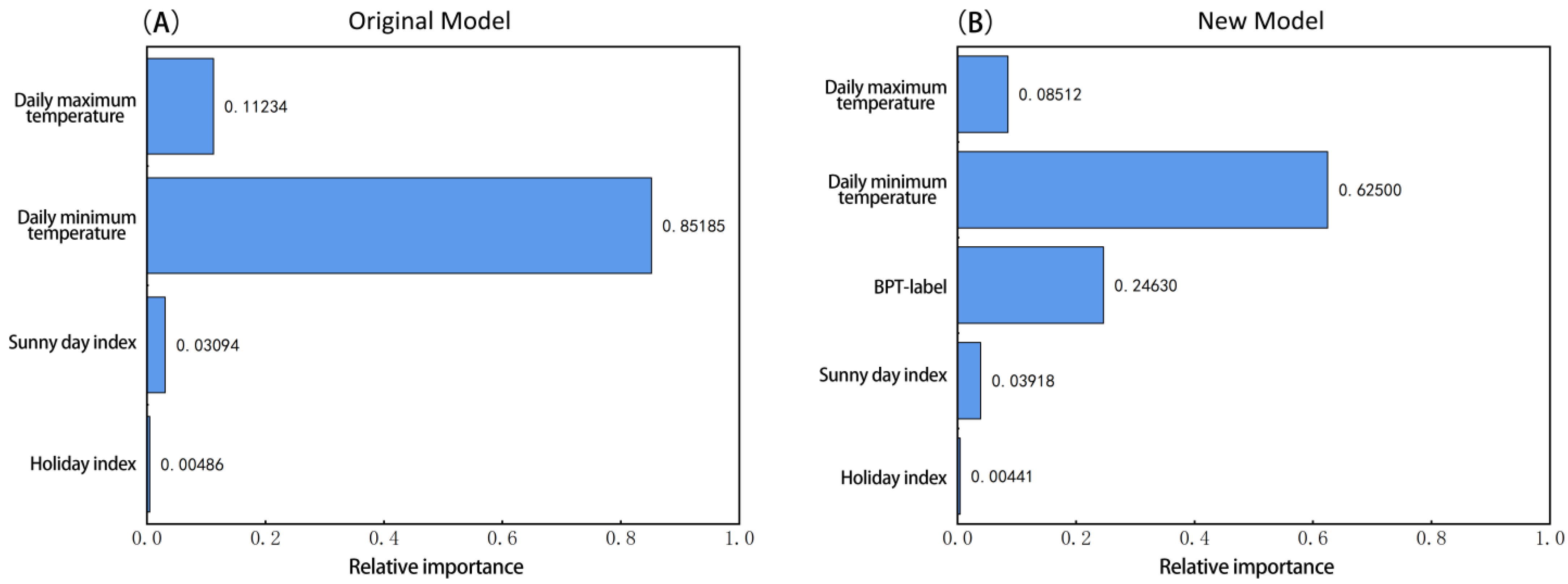
4.2. Importance Analysis of Input Variables

This study analyzes the building energy consumption of an apartment building in Xiamen, China. Four explanatory variables were collected and five data-driven models were established to predict the building’s daily energy consumption. A balance point temperature label was later added to determine the impact of its inclusion on the accuracy of the data-driven model predictions. The importance of each input variable, i.e., the degree of influence on energy consumption, was analyzed using the feature importance method based on the RF algorithm.
Figure 9A shows the importance of each variable in the original model. The impact of daily minimum air temperature (85%) on energy consumption is far greater than that of other variables, playing a dominant role, and its importance is much greater than that of daily maximum temperature (11%). This is an interesting phenomenon. The importance of the holiday index is almost negligible, while the importance of the sunny day index accounts for 3%. With the addition of the BPT label, the importance of the minimum temperature has decreased, and its partial importance has been shared by the balance point temperature, while the importance of other variables has remained largely unchanged, as shown in Figure 9B. Finally, the importance of the BPT label accounts for 25%, and the importance of the minimum temperature has dropped to 62.5%. Therefore, the balance point temperature cannot be ignored in the prediction model of building daily energy consumption. This also explains why adding the BPT label to the input variables in the previous experiment greatly improves the prediction accuracy of the prediction model.
It is worth noting that in the daily energy consumption prediction model, both the daily minimum and maximum temperatures are considered temperature information in meteorological data. The importance of the daily minimum temperature dominates, while the daily maximum temperature is not as important. This indicates that the daily minimum temperature dominates people’s main thermal sensation on that day, rather than the daily maximum temperature. For example, if the minimum temperature of a day is very low, even if the maximum temperature at noon is high, people will still consider it a cold season and usually will not turn on the air conditioning briefly at noon, which means that the energy consumption of that day will not increase significantly. On the contrary, if the minimum temperature of the day is also high, people will feel that it is a hot season and choose to use air conditioning, which significantly increases energy consumption.

5. Discussion

Given the widespread lack of information on building data, researchers need to continue exploring how to accurately predict building energy consumption with relatively limited data. This study summarizes two potential strategies that can improve the predictive performance of building energy models: (1) mining efficient feature variables and (2) selecting and optimizing models. Specific discussions are as follows.
  • The current data-driven building energy consumption prediction models tend to focus on selecting input feature variables related to meteorological and building parameters. In order to discover more feature variables that influence building energy consumption, researchers have deployed numerous sensors within and around buildings and constructed energy management systems. However, the excessive monitoring data has instead increased the difficulty of analysis, as most input variables have minimal impact on building energy consumption, such as the holiday index in this study (which had a feature importance of only 0.4%). Therefore, improving feature variable selection can involve more comprehensive consideration of building attributes and environmental factors, using more advanced feature selection techniques, and exploring new feature variable methods. This article is the first study to use the balance point temperature label as a feature variable. Through the data analysis, it was found that the balance point temperature label can significantly improve the performance of the building energy consumption prediction model, with an importance of about 25%.
  • Building energy consumption models can be modeled based on different machine learning algorithms, such as BPNN, RF, SVR, LASSO, KNN, etc., as used in this study. Different algorithms are suitable for different datasets and problems, so selecting the appropriate algorithm is crucial to improve predictive performance. This article suggests through the analysis of a case in Xiamen that when there are sufficient input features, BPNN is optimal, and when input features are insufficient, KNN is best. However, in actual situations, there is no quantitative standard for whether input feature data is sufficient, but rather a subjective judgment based on the researcher’s experience. Therefore, before conducting predictive analysis on a specific building case, potential models should be screened instead of using a single prediction model or method that the researcher is good at. In addition, model optimization can also improve predictive performance. Hyper-parameters should be optimized before model application.
As predictive models continue to deepen and optimize, the algorithms themselves have become more mature. However, even so, the limitations of machine learning-based algorithms should also be discussed.
  • Data quality issues: The predictive performance of building energy consumption models is influenced by the quality and quantity of input data. If the data contains missing values, outliers, or noise, the predictive performance of the model will be affected.
  • Transferability issues: The predictive performance of building energy consumption models may be influenced by transferability issues between datasets. This is because building characteristics and environmental factors may vary across different geographic locations and time periods, thus limiting the predictive performance of the model.
  • Interpretability issues: Machine learning models are often considered “black box” models, making it difficult to explain the reasons for their predicted results. This may limit the practical application of the model.
Finally, it needs to be further explained that the experiments in this article were conducted in Xiamen, China, which belongs to the climate zone of hot summer and warm winter. For buildings located in other geographical locations, the number and size of the balance point temperature may be different, but the statistical algorithm proposed in this article can be used as a reference and reference.

6. Conclusions

With the in-depth development of building energy performance evaluation, abnormal energy consumption diagnosis, and building energy conservation, energy consumption prediction has become the research basis of these works. This article analyzed the daily power consumption data of a certain apartment community in Xiamen and improved the prediction accuracy of five data-driven models using the balance point temperature label. The method was applied and verified in practical tests, and the following conclusions were drawn:
  • This article proposes a statistical algorithm for calculating the balance point temperature and identifies the balance point temperature of a residential building in Xiamen, China as 22.2 °C. Significant differences in the correlation between temperature and building energy consumption exist around this balance point temperature.
  • Adding the balance point temperature label to the input variables can significantly improve the daily energy consumption prediction accuracy of data-driven models. The R2 values of the BPNN model increased by 0.3448, SVR increased by 0.2262, RF increased by 0.2165, LASSO increased by 0.3066, and KNN increased by 0.1440.
  • In the task of daily energy consumption prediction, the prediction accuracy of data-driven models varies under different input data conditions. When the input variable data is insufficient, the prediction performance from high to low is KNN, RF, SVR, BPNN, and LASSO. When the input variable data is sufficient, the prediction performance is in the order of BPNN, SVR, KNN, RF, and LASSO.
  • Among the input variables of the daily energy consumption prediction model, the dominant variable is the daily minimum temperature, which is much more important than the daily maximum temperature. The balance point temperature label is crucial in the prediction model and accounts for 25% of the importance.

Author Contributions

Conceptualization, H.Y.; Formal analysis, H.Y.; Investigation, H.Y.; Methodology, H.Y.; Resources, M.R.; Software, H.Y.; Supervision, M.R.; Validation, M.R. and H.F.; Visualization, H.Y.; Writing—original draft, H.Y.; Writing—review & editing, M.R. and H.F. All authors have read and agreed to the published version of the manuscript.

Funding

This research was funded by National Natural Science Foundation of China, grant number 51678254.

Data Availability Statement

Not applicable.

Conflicts of Interest

The authors declare no conflict of interest.

References

  1. Anderson, J.E.; Wulfhorst, G.; Lang, W. Energy analysis of the built environment—A review and outlook. Renew. Sustain. Energy Rev. 2015, 44, 149–158. [Google Scholar] [CrossRef]
  2. Tam, V.W.; Le, K.N.; Tran, C.N.; Illankoon, I.C.S. A review on international ecological legislation on energy consumption: Greenhouse gas emission management. Int. J. Constr. Manag. 2021, 21, 631–647. [Google Scholar] [CrossRef]
  3. Du, K.; Xie, J.; Khandelwal, M.; Zhou, J. Utilization Methods and Practice of Abandoned Mines and Related Rock Mechanics under the Ecological and Double Carbon Strategy in China—A Comprehensive Review. Minerals 2022, 12, 1065. [Google Scholar] [CrossRef]
  4. Deng, H.; Xie, C. An improved particle swarm optimization algorithm for inverse kinematics solution of multi-DOF serial robotic manipulators. Soft Comput. 2021, 25, 13695–13708. [Google Scholar] [CrossRef]
  5. Zhang, J.-R.; Zhang, J.; Lok, T.-M.; Lyu, M.R. A hybrid particle swarm optimization–back-propagation algorithm for feedforward neural network training. Appl. Math. Comput. 2007, 185, 1026–1037. [Google Scholar] [CrossRef]
  6. Chu, Y.; Yuan, H.; Jiang, S.; Fu, C. Neural Network-Based Reference Block Quality Enhancement for Motion Compensation Prediction. Appl. Sci. 2023, 13, 2795. [Google Scholar] [CrossRef]
  7. Raza, A.; Ullah, N.; Khan, J.A.; Assam, M.; Guzzo, A.; Aljuaid, H. DeepBreastCancerNet: A Novel Deep Learning Model for Breast Cancer Detection Using Ultrasound Images. Appl. Sci. 2023, 13, 2082. [Google Scholar] [CrossRef]
  8. Amber, K.P.; Aslam, M.W.; Mahmood, A.; Kousar, A.; Younis, M.Y.; Akbar, B.; Chaudhary, G.Q.; Hussain, S.K. Energy consumption forecasting for university sector buildings. Energies 2017, 10, 1579. [Google Scholar] [CrossRef]
  9. Yang, H.; Ran, M.; Zhuang, C. Prediction of Building Electricity Consumption Based on Joinpoint–Multiple Linear Regression. Energies 2022, 15, 8543. [Google Scholar] [CrossRef]
  10. Yang, J.; Ning, C.; Deb, C.; Zhang, F.; Cheong, D.; Lee, S.E.; Sekhar, C.; Tham, K.W. k-Shape clustering algorithm for building energy usage patterns analysis and forecasting model accuracy improvement. Energy Build. 2017, 146, 27–37. [Google Scholar] [CrossRef]
  11. Bouktif, S.; Fiaz, A.; Ouni, A.; Serhani, M.A. Multi-sequence LSTM-RNN deep learning and metaheuristics for electric load forecasting. Energies 2020, 13, 391. [Google Scholar] [CrossRef]
  12. Liang, Y.; Pan, Y.; Yuan, X.; Jia, W.; Huang, Z. Surrogate modeling for long-term and high-resolution prediction of building thermal load with a metric-optimized KNN algorithm. Energy Built Environ. 2022. [CrossRef]
  13. Ding, Z.; Wang, Z.; Hu, T.; Wang, H. A Comprehensive Study on Integrating Clustering with Regression for Short-Term Forecasting of Building Energy Consumption: Case Study of a Green Building. Buildings 2022, 12, 1701. [Google Scholar] [CrossRef]
  14. Javed, F.; Arshad, N.; Wallin, F.; Vassileva, I.; Dahlquist, E. Forecasting for demand response in smart grids: An analysis on use of anthropologic and structural data and short term multiple loads forecasting. Appl. Energy 2012, 96, 150–160. [Google Scholar] [CrossRef]
  15. Li, Q.; Meng, Q.; Cai, J.; Yoshino, H.; Mochida, A. Applying support vector machine to predict hourly cooling load in the building. Appl. Energy 2009, 86, 2249–2256. [Google Scholar] [CrossRef]
  16. Sholahudin, S.; Han, H. Simplified dynamic neural network model to predict heating load of a building using Taguchi method. Energy 2016, 115, 1672–1678. [Google Scholar] [CrossRef]
  17. Ding, Y.; Zhang, Q.; Yuan, T. Research on short-term and ultra-short-term cooling load prediction models for office buildings. Energy Build. 2017, 154, 254–267. [Google Scholar] [CrossRef]
  18. Ding, Y.; Zhang, Q.; Yuan, T.; Yang, K. Model input selection for building heating load prediction: A case study for an office building in Tianjin. Energy Build. 2018, 159, 254–270. [Google Scholar] [CrossRef]
  19. Fan, C.; Xiao, F.; Zhao, Y. A short-term building cooling load prediction method using deep learning algorithms. Appl. Energy 2017, 195, 222–233. [Google Scholar] [CrossRef]
  20. Bracale, A.; Carpinelli, G.; De Falco, P.; Hong, T. Short-term industrial reactive power forecasting. Int. J. Electr. Power Energy Syst. 2019, 107, 177–185. [Google Scholar] [CrossRef]
  21. Krese, G.; Lampret, Ž.; Butala, V.; Prek, M. Determination of a Building’s balance point temperature as an energy characteristic. Energy 2018, 165, 1034–1049. [Google Scholar] [CrossRef]
  22. Hao, Z.; Xie, J.; Zhang, X.; Liu, J. Simplified Model of Heat Load Prediction and Its Application in Estimation of Building Envelope Thermal Performance. Buildings 2023, 13, 1076. [Google Scholar] [CrossRef]
  23. Aranda, A.; Ferreira, G.; Mainar-Toledo, M.; Scarpellini, S.; Sastresa, E.L. Multiple regression models to predict the annual energy consumption in the Spanish banking sector. Energy Build. 2012, 49, 380–387. [Google Scholar] [CrossRef]
  24. Historical Weather in Xiamen. Available online: https://q-weather.info/weather/59134/history/ (accessed on 21 September 2022).
  25. General Office of the State Council. Notice of the General Office of the State Council on the Arrangement of Some Holidays in 2023. Available online: http://www.gov.cn/zhengce/content/2022-12/08/content_5730844.htm (accessed on 21 September 2022).
  26. Bourdeau, M.; Zhai, X.Q.; Nefzaoui, E.; Guo, X.; Chatellier, P. Modeling and forecasting building energy consumption: A review of data-driven techniques. Sustain. Cities Soc. 2019, 48, 101533. [Google Scholar] [CrossRef]
  27. Chen, Z.; Chen, Y.; Xiao, T.; Wang, H.; Hou, P. A novel short-term load forecasting framework based on time-series clustering and early classification algorithm. Energy Build. 2021, 251, 111375. [Google Scholar] [CrossRef]
  28. Cheadle, C.; Vawter, M.P.; Freed, W.J.; Becker, K.G. Analysis of microarray data using Z score transformation. J. Mol. Diagn. 2003, 5, 73–81. [Google Scholar] [CrossRef]
  29. Hecht-Nielsen, R. Theory of the backpropagation neural network. In Neural Networks for Perception; Elsevier: Amsterdam, The Netherlands, 1992; pp. 65–93. [Google Scholar]
  30. Breiman, L. Bagging predictors. Mach. Learn. 1996, 24, 123–140. [Google Scholar] [CrossRef]
  31. Deb, S.; Gao, X.-Z. Prediction of Charging Demand of Electric City Buses of Helsinki, Finland by Random Forest. Energies 2022, 15, 3679. [Google Scholar] [CrossRef]
  32. Janitza, S.; Strobl, C.; Boulesteix, A.-L. An AUC-based permutation variable importance measure for random forests. BMC Bioinform. 2013, 14, 119. [Google Scholar] [CrossRef]
  33. Strobl, C.; Boulesteix, A.-L.; Kneib, T.; Augustin, T.; Zeileis, A. Conditional variable importance for random forests. BMC Bioinform. 2008, 9, 307. [Google Scholar] [CrossRef]
  34. Cortes, C.; Vapnik, V. Support-vector networks. Mach. Learn. 1995, 20, 273–297. [Google Scholar] [CrossRef]
  35. Kukreja, S.L.; Löfberg, J.; Brenner, M.J. A least absolute shrinkage and selection operator (LASSO) for nonlinear system identification. IFAC Proc. Vol. 2006, 39, 814–819. [Google Scholar] [CrossRef]
  36. Peterson, L.E. K-nearest neighbor. Scholarpedia 2009, 4, 1883. [Google Scholar] [CrossRef]
  37. ASHRAE Guideline 14: Measurement of Energy, Demand, and Water Savings; ASHRAE: Atlanta, GA, USA, 2014.
  38. Garreta, R.; Moncecchi, G. Learning Scikit-Learn: Machine Learning In Python; Packt Publishing Ltd.: Birmingham, UK, 2013. [Google Scholar]
  39. Said, S.A.M.; Habib, M.A.; Iqbal, M.O. Database for building energy prediction in Saudi Arabia. Energy Convers. Manag. 2003, 44, 191–201. [Google Scholar] [CrossRef]
  40. Verbai, Z.; Lakatos, Á.; Kalmár, F. Prediction of energy demand for heating of residential buildings using variable degree day. Energy 2014, 76, 780–787. [Google Scholar] [CrossRef]
Figure 1. Research outline of the study.
Buildings 13 01423 g001
Figure 2. Photograph of the selected apartment buildings.
Buildings 13 01423 g002
Figure 3. Daily temperature parameters.
Buildings 13 01423 g003
Figure 4. Average air temperature versus average daily electricity consumption.
Buildings 13 01423 g004
Figure 5. The plot of change in R2 values.
Buildings 13 01423 g005
Figure 6. Model at optimal R2 value.
Buildings 13 01423 g006
Figure 7. Grid search for optimal parameters: (a) BPNN, (b) RF, (c) SVR, (d) LASSO, (e) KNN.
Buildings 13 01423 g007
Figure 8. Comparison of measured and forecasted value for the data-driven models with or without BPT label.
Buildings 13 01423 g008
Figure 9. Importance of input variables.
Buildings 13 01423 g009
Table 1. Detailed information on the building and room.
ItemDetail
BuildingBuilding typeApartment
LocationXiamen, China
Build time2014s
Floors9
RoomRoom area 25.33 m2
Height3.10 m
Led tubeModel: TSZJD2-T5-28W
FanModel: FSLD-40
Air conditionerModel: KF-35 GW/S (35355) A1-N1
SocketMaximum load: 2 kW
Table 2. Dependent and explanatory variables for this study.
VariablesSymbolContentType
Dependent variableYDaily average electricity consumptionContinuous variable
Explanatory variable 1x1Holiday indexProxy variable
Explanatory variable 2x2Sunny day indexProxy variable
Explanatory variable 3x3Daily minimum temperatureContinuous variable
Explanatory variable 4x4Daily maximum temperatureContinuous variable
Table 3. Parameters optimization result and performance of different models.
ModelParametersOptimal ValueBest Cross-Validation Score (R2)
BPActivationrelu0.8484
Learning rate0.01
Hidden Layers3
Hidden Nodes50
SVRKernel function RBF0.7436
C0.8
gamma0.23
RFMax depth50.8350
Number of trees20
LASSOalpha0.0010.6558
KNNK30.8233
P3
weightsdistance
Table 4. Prediction metrics for the models.
ModelR2CV−RMSE (%)NMBE (%)
OriginalNewOriginalNewOriginalNew
TrainTestTrainTestTrainTestTrainTestTrainTestTrainTest
BPNN0.83510.49460.92040.839354.0356.3837.5437.1818.8110.002.680.94
SVR0.76410.51510.82790.741348.7764.5941.6547.1810.7174.188.6854.51
RF0.87330.52140.91710.737935.7464.1628.9147.4846.1759.2517.8838.55
LASSO0.61340.21670.67590.523262.4282.0957.1664.0424.0084.7626.0038.23
KNN0.99970.59420.99990.73821.8459.080.9547.460.0058.640.0060.92
Table 5. Result of t-test between the results with/without BPT label.
BPSVRRFLASSOKNN
p-value0.0000.0000.0000.0000.000
Disclaimer/Publisher’s Note: The statements, opinions and data contained in all publications are solely those of the individual author(s) and contributor(s) and not of MDPI and/or the editor(s). MDPI and/or the editor(s) disclaim responsibility for any injury to people or property resulting from any ideas, methods, instructions or products referred to in the content.

