Abstract
The impact effect is a crucial issue in civil engineering and has received considerable attention for decades. For the first time, this study develops hybrid machine learning models that integrate the novel Extreme Gradient Boosting (XGB) model with Particle Swam Optimization (PSO), Grey Wolf Optimizer (GWO), Moth Flame Optimizer (MFO), Jaya (JA), and Multi-Verse Optimizer (MVO) algorithms for predicting the permanent transverse displacement of circular hollow section (CHS) steel members under impact loads. The hybrid machine learning models are developed using data collected from 357 impact tests of CHS steel members. The efficacy of hybrid machine learning models is evaluated using three performance metrics. The results show that the GWO-XGB model achieves high accuracy and outperforms the other models. The values of R2, RMSE, and MAE obtained from the GWO-XGB model for the test set are 0.981, 2.835 mm, and 1.906 mm, respectively. The SHAP-based model explanation shows that the initial impact velocity of the indenter, the impact mass, and the ratio of impact position to the member length are the most sensitive parameters, followed by the yield strength of the steel member and the member length; meanwhile, member diameter and member thickness are the parameters least sensitive to the permanent transverse displacement of CHS steel members. Finally, this study develops a web application tool to help rapidly estimate the permanent transverse displacement of CHS steel members under impact loads.
1. Introduction
Nowadays, many cross-section types are employed for construction members in steel structures. Due to its excellent properties, the circular hollow section (CHS) is considered one of the most used sections [1]. The CHS steel member increases the strength-to-weight ratio during serviceability. In addition, it improves structural efficiency and allows for a longer member span. Consequently, CHS steel members are employed in various well-designed and highly efficient steel structures worldwide, such as offshore platforms, subsea pipelines, conveyor columns, overpass columns, building garages, and airport terminals. Generally, these structures can be subject to impact loads during their design life [2,3]. For example, in offshore platforms and subsea pipelines, accident loads often lead to tubular structures failing due to dropped objects or collisions [4,5]. However, the structures may be subjected to impact loads from accidental or intentional impacts, such as collisions with vehicles, or terrorist attacks [2,6]. In the event of an impact, structures will gradually lose their bearing capacity and may even collapse without warning.
Several experimental and numerical studies have been conducted to determine structural members’ behavior and failure modes under the impact load [7,8,9,10,11,12,13,14,15,16,17]. Moreover, several building codes and previous studies have provided guidelines for structures under impact loads [2,18,19], and many studies have developed analytical procedures (i.e., plastic collapse mechanism theory) to describe the mechanical behavior of solid metal and hollow sections [20,21,22,23,24,25,26]. Nevertheless, they do not provide detailed guidelines for such types of CHS steel members under impact loads [27,28]. They are usually designed from a mechanical perspective and do not adapt readily to routine civil-structural design [2]. Since impact behavior is a complex engineering task, developing a theoretical model for a specific problem under impact load is challenging.
Machine learning (ML) methods have recently received considerable attention in civil engineering [29,30,31,32,33,34,35]. Among various regression ML algorithms, the Extreme Gradient Boosting (XGB) algorithm has recently gained substantial popularity in modeling several nonlinear mechanical behaviors for classification and regression [36,37,38,39,40,41,42,43]. The XGB provides good prediction performance by reducing overfitting and controlling model complexity through its built-in regularization [44,45]. For example, Feng et al. [46] have shown that the XGB model could predict the shear strength of reinforced concrete deep beams better than other ML models. Additionally, the XGB model has been shown to perform better than other ML models for several structural engineering problems [47,48,49]. However, it should be noted that ML algorithms require hyperparameters to be set before they can be run. Therefore, selecting appropriate hyperparameters of ML models for a specific dataset is critical because the performance of ML models depends on their hyperparameter settings.
In recent decades, metaheuristic algorithms have been used as one of the most popular research topics in many optimization fields, including the optimum design of truss and frame structures [50,51,52,53] or damage detection [54,55,56] because of their simplicity and flexibility, derivative-free mechanism, low dependency on problems, and local optima avoidance. In contrast to gradient-based methods, metaheuristic algorithms are more efficient because they are simple and easy to use [57]. To enhance the ability of ML models to generalize, an optimal set of hyperparameters must be determined. In recent years, metaheuristic algorithms have gained popularity as an alternative method for fine-tuning the hyperparameters of ML models, since they can improve the performance of the optimization strategy [45,58,59,60,61,62].
Although metaheuristic algorithms have been used for different engineering problems, there has been no comprehensive evaluation or comparison of metaheuristic algorithms hybridized with the XGB models for predicting the permanent transverse displacement () of CHS steel members. For the first time, this study compares the performance of several hybrid models by combining the XGB model with the PSO, GWO, MFO, JA, and MVO algorithms for predicting the of CHS steel members. The hybrid ML models are trained and tested on an experimental database collected from the literature and evaluated using various performance metrics. The performance of hybrid ML models is assessed to find the best model for predicting the of CHS steel members. Finally, a web application is developed that can provide this prediction quickly and repeatedly.
2. Data Collection
The full-clamped CHS steel members under transverse impact loading using drop-weight tests are shown in Figure 1. The critical parameters of the specimens are the member length (), the member diameter (), the member thickness (), the ratio of impact position to the member length (), the yield strength of the steel member (), the impact mass (), the initial impact velocity of the indenter (), and .
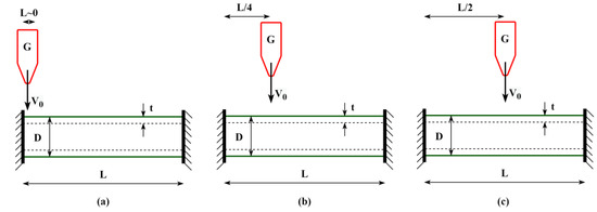
Figure 1.
A full-clamped CHS steel member subjected to impact loading (a) near a support; (b) at one-quarter span; (c) at mid-span.
According to Jones et al. [63] and Jones and Shen [23], the idealized deformed cross-section of full-clamped CHS steel members at the point of impact is shown in Figure 2, where is the original mean radius of a member, is the local displacement, is the global displacement, and is the the maximum outside diameter of a dented cross-section. The dented zone is somewhat symmetrical about the impact plane for the middle- and quarter-span impact tests; meanwhile, it is no longer symmetrical about the impact plane for the impact position close to support. This method idealizes a deformed cross-section to estimate the local displacement and global displacement of the permanent transverse displacement from the experimental measurements of the final cross-section [4]. After an impact test, the is measured at the indentation point on the member prior to unclamping and removal from the rig. After removal, the is measured again while supporting the member on two knife-edged vee blocks spaced apart (representing the same support span). It was found that there was very little difference (0.5 mm maximum) between the two measurements, so an average value was taken [64]. It is worth noting that the is the main parameter used to estimate the total plastic energy absorbed in a member [4].
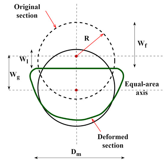
Figure 2.
The idealized deformed cross-section [23,64].
This study collects a comprehensive database of 357 experimental tests of full-clamped CHS steel members under impact load. The database is collected mainly from the studies of Jones et al. [63], Chen and Shen [64], and Jones and Birch [65]. Jones et al. [63] conducted 130 tests of fully clamped CHS steel members under lateral impact load, considering several diameters, lengths, and velocities. Chen and Shen [64] conducted 226 tests of CHS steel members under lateral impact load. Jones and Birch [65] conducted 54 impact tests on CHS steel members under impact load. The database deals with outliers, duplicates, and missing values. As a result, the final database of the 357 data points used in this study is summarized in Table 1.

Table 1.
Statistical properties of experimental data.
The distributions of the input parameters (, , , , , , and ) and the output parameter () are shown in Figure 3. Additionally, Figure 4 shows the correlation matrix of the variables. Correlation values between the independent variables (, , , , , , and ) and dependent variable () are 0.48, 0.50, 0.27, 0.52, 0.0, 0.43, and 0.69, respectively. It can be seen that the is strongly correlated with ; meanwhile, the variables , , , , and are moderately correlated with , while is almost independent of the .
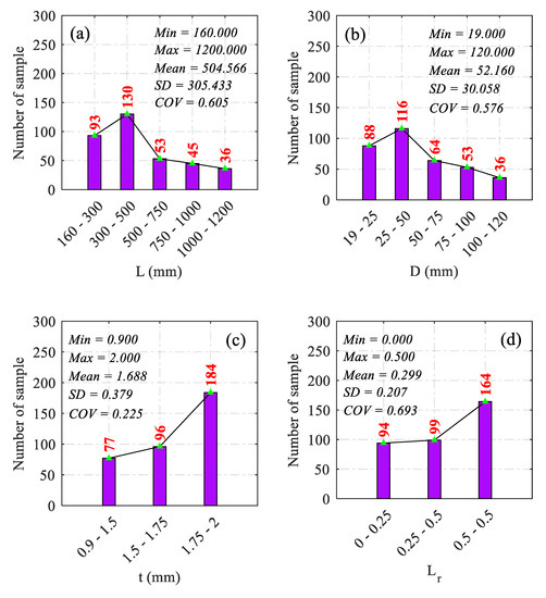
Figure 3.
Distribution of input and output parameters: (a) the member length, (b) the member diameter, (c) the member thickness, (d) the ratio of impact position to the member length, (e) the yield strength of the steel member, (f) the impact mass, (g) the initial impact velocity of the indenter, and (h) the permanent transverse displacement.
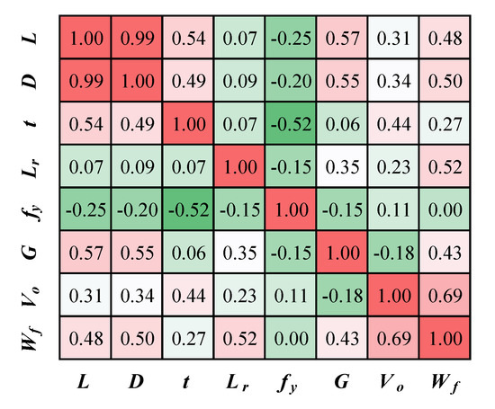
Figure 4.
Pearson correlation between input and output parameters.
3. Machine Learning and Optimization Algorithms
This study uses five popular metaheuristic algorithms (i.e., PSO, GWO, MFO, JA, and MVO) coupled with the XGB model to investigate the prediction of the of CHS steel members under impact loading. Due to space limitations, brief descriptions of these algorithms are presented in this section. The information needed on selected ML algorithms in this study can be found in previous references [66,67].
3.1. Extreme Gradient Boosting (XGB)
Chen and Guestrin [68] developed the XGB based on the gradient boosting algorithm proposed by Friedman et al. [69]. The XGB is a highly optimized and parallelized version of the gradient boosting algorithm. For each iteration of the XGB, the residual is used to calibrate the previous predictor. Additionally, the XGB uses an approximate algorithm to find the best-split points. The XGB is characterized by some critical features [68]: parallelization (can train with multiple CPU cores), regularization (contains several regularization penalties to avoid overfitting and generalize adequately), scalability (can run distributed and process enormous amounts of data), effective tree pruning (can make the splitting up to the specified max_depth value and then start pruning the tree backward), and missing value handling (has an in-built capability to handle missing values).
The XGB is superior to gradient boosting in many respects (i.e., the smarter breakup of trees, random hidden node generation, shorter leaf nodes, and out-of-core predictions) [69]. Moreover, the XGB adds the regularization term in the loss function to avoid overfitting. In addition, the training time is drastically reduced by parallelizing the entire boosting process in the XGB [68]. Therefore, the XGB can be used for many engineering simulations and provides fast and reliable results [70,71,72]. The details of the XGB can be found in [60,72].
3.2. Particle Swarm Optimization (PSO)
Kennedy and Eberhart developed the PSO algorithm [73], which is inspired by the complex social behavior of flocking birds. The basic idea of PSO is to share the food place between groups of birds (also called particles). Particles have two important indexes: (I) the fitness value and (II) velocity. PSO creates a population of random particles and moves them using velocity in the search space in every iteration. This velocity term refers to the best-found solution and each particle’s best experience. The next step would be to repeat this procedure to find a more promising search area and a better solution. The details of the PSO algorithm can be found in [73].
3.3. Grey Wolf Optimizer (GWO)
Mirjalili et al. proposed GWO [74] inspired by the grey wolves’ social hierarchy and hunting behavior. To represent the social hierarchy (leadership), the grey wolves’ population is divided into four levels: alpha () is at the top of the hierarchy, leading the group; beta () is next to in the social hierarchy to help in making decisions and other activities; omega () is dominated by other wolves; and delta () dominates but submits to and . includes caretakers, hunters, sentinels, scouts, and elders [74]. The hunting behavior is divided into four steps: searching, encircling, hunting, and attacking the prey. The details of the GWO algorithm can be found in [74].
3.4. Moth Flame Optimizer (MFO)
Mirjalili developed an MFO based on moths’ navigation method through the night [75]. The main inspiration of MFO is the attraction and spiral movement of moths around artificial light sources. This spiral movement occurs because moths are easily tricked by artificial light. Due to the extremely short distance, a moth fails to keep a fixed angle when it sees an artificial light. Therefore, a deadly spiral path is generated in the MFO. Using MFO, a given optimization problem can be reasonably approximated to its global optimum. The details of the MFO algorithm can be found in [75].
3.5. Jaya Algorithm (JA)
JA is a simple yet powerful algorithm introduced by Rao [76]. The JA has a few specific parameters (i.e., population size and termination condition) without algorithm-specific parameters being set in advance, which makes it easy to implement. In each iteration, JA aims to avoid the worst solution and find the best one. The details of the JA algorithm can be found in [76].
3.6. Multi-Verse Optimizer (MVO)
MVO was proposed by S. Mirjalili et al. [77] and inspired by the multi-verse theory in physics. The MVO explains how the Big Bang creates multiple universes and how they interact through the white hole, black hole, and wormhole. MVO utilizes the concepts of a white hole and a black hole to explore the wormhole and exploit the search spaces to formulate a population-based algorithm. In the MVO, population size represents the number of universes, a universe is a solution, and objects in the universe are variables. Additionally, each solution has an inflation rate (fitness value) that represents the quality of the solution. The details of the MWO algorithm can be found in [77].
4. Development of Hybrid ML Models
Three performance metrics are used in this study to evaluate the ML models. They are the correlation coefficient (), the root mean square error (), and the mean absolute error (). , , and are expressed as follows.
where is the number of samples, is the average of actual values, and and are the actual and the predicted values, respectively.
Figure 5 summarizes the entire process of developing the hybrid ML models used in this study. First, the experimental database is collected and randomly divided into training and test sets. Then, the training set is used to develop the ML models using the K-fold cross-validation (CV) technique. Previous studies have explained the idea of the K-fold CV in detail [32,45,78]. This study adopts a 5-fold CV into the training data set. In the next step, the optimization algorithms are used to find the optimal hyperparameters based on the average MAE value over the testing folds. This process is iterated by changing the training-test ratio and population size. Therefore, many models are built and evaluated using three metrics (R2, RMSE, and MAE) to adopt the best hybrid ML model. Finally, a new prediction can be obtained. Based on the best hybrid model, the contribution of the input variable to output prediction is performed using the SHAP method. In addition, a web application is developed to predict the rapidly. The following sections introduce detailed descriptions of the procedure.
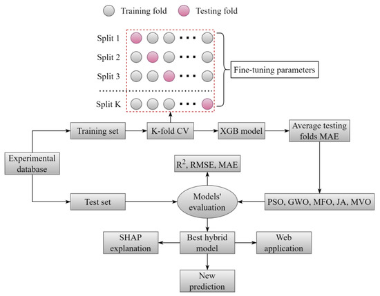
Figure 5.
Flowchart of the development of hybrid ML models.
Considering the main factors affecting the transverse displacement mentioned in Section 3, the input variables of the ML models are the , , , , , , and , and the output is the . ML models are significantly influenced by the dataset division ratio [32,45,66,79,80,81,82,83]. To investigate the effect of database division on ML model performance, this study uses seven ratios of 0.60:0.40, 0.65:0.35, 0.70:0.30, 0.75:0.25, 0.80:0.20, 0.85:0.15, and 0.90:0.10 to select the best one for the current database.
It is worth emphasizing that hyperparameters are the key to XGB models. Therefore, finding the best combination of hyperparameters for XGB models plays a crucial role. Table 2 presents the hyperparameters and ranges of the XGB model applied in this study.
Table 2.
Hyperparameters of XGB algorithms.
5. Results and Discussions
5.1. Comparison of Performance of Different ML Models
This study develops many hybrid models that combine the PSO, GWO, MFO, JA, and MVO algorithms with the XGB model, considering the effect of population size and training-test ratio. The detailed results are presented in the Supplementary Materials. A comparison of performance metrics on a test set is used to evaluate the ML models’ performance on unseen data. Accordingly, each evaluation metric is scored from 1 to 35, corresponding to the training ratios and population sizes. It is noted that the higher the R2 value is, the higher the score is, and the higher the RMSE and MAE values, the lower the score. When the value of the evaluation metric obtained by different ML models is the same, the scoring is equal. After that, all evaluation metric score values are summed up to get the final score of each ML model. The best results of the PSO-XGB, GWO-XGB, MFO-XGB, JA-XGB, and MVO-XGB models are highlighted in bold in the tables in the Supplementary Materials. Table 3 and Figure 6 show the performance of these models based on the R2, RMSE, and MAE values. In addition, their results are compared with those of the default XGB model to demonstrate the efficacy of the optimization algorithm. Generally, the training performance is better than the test for all models. In the GWO-XGB model, however, there is a minor difference between training and test sets, so there is little overfitting. The GWO-XGB provides (0.997 and 0.981), (1.207 mm and 2.835 mm), and (0.797 mm and 1.906 mm) for R2, RMSE, and MAE in the training set and test set, respectively. In contrast, the default XGB model significantly differs between training and test performances. The default XGB obtains (1.0 and 0.954), (0.174 mm and 4.248 mm), and (0.094 mm and 2.377 mm) for R2, RMSE, and MAE in the training set and test set, respectively.
Table 3.
Performance of ML models.
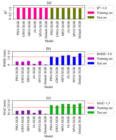
Figure 6.
Performance of ML models: (a) R2 values, (b) RMSE values, and (c) MAE values.
It is observed that all hybrid ML models perform better than the default XGB model in the test set. Compared with the default XGB model, R2 increased by (2.201%, 2.830%, 1.572%, 1.258%, and 2.201%), RMSE decreased by (27.095%, 33.263%, 19.185%, 15.419%, and 28.413%), and MAE reduced by (15.061%, 19.815%, 3.912%, 4.081%, and 9.466%), respectively, in the PSO-XGB, GWO-XGB, MFO-XGB, JA-XGB, and MVO-XGB models. This indicates that the PSO, GWO, MFO, JA, and MVO algorithms can significantly enhance the capacity of the XGB model. Overall, it seems that the GWO improved the XGB model over the other optimization algorithms in this study.
According to the results, the GWO-XGB model with a population size of 150 and a training-test ratio of 0.90:0.10 performs better than the other ML models; meanwhile, the default XGB model has the worst prediction performance. The optimal hyperparameters of the best GWO-XGB model are shown in Table 2.
Figure 7 compares the predicted and the actual values of the PSO-XGB, GWO-XGB, MFO-XGB, JA-XGB, MVO-XGB, and default XGB models. In this figure, the vertical axis represents predicted values of , and the horizontal axis represents observed values of .
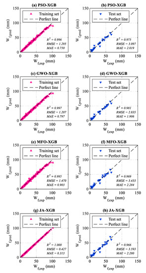
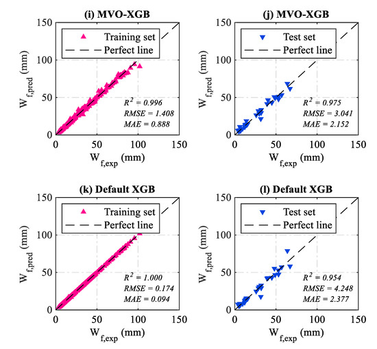
Figure 7.
Scatter plots of different ML models.
5.2. Model Explanation
In this section, the Shapley additive explanations (SHAP) method [84] is used to explain individual and global prediction of . The effect of the Shapley value on the prediction value is shown in Figure 8. Shapley values are like arrows pointing towards a predicted value that either increases (positive value) or decreases (negative value).
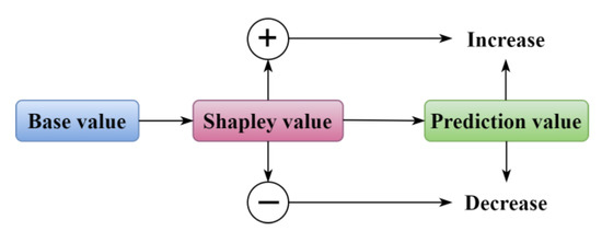
Figure 8.
Effect of Shapley value.
Figure 9a shows the global importance factors of the seven input variables for the prediction. The feature with a larger absolute summation of Shapley values is more important. It can be seen that the and have a significant influence on the prediction, followed by , , , , and
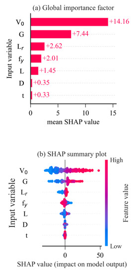
Figure 9.
Global importance factors.
Figure 9b shows the SHAP summary plot. Each point on the graph represents the Shapley value for each specimen. The red point on the right-hand side of the plot indicates a positive correlation with the , while the red point on the left-hand side indicates a negative correlation. Accordingly, when , , and increase, the increases. In contrast, the decreases if the increases. Meanwhile, the , , and are less effective and unclear on predictions.
Figure 10a shows the Shapley values of a typical prediction using the GWO-XGB model for a specimen with mm, mm, mm, , MPa, kg, and m/s. It can be seen in Figure 10a that the prediction (60.785 mm) is larger than the base value (29.385 mm). The , , , , and parameters, shown in red, increase the base value; meanwhile, other parameters ( and ), depicted in blue, decrease the base value. Among them, the most crucial variable is . For a specimen in Figure 10b with mm, mm, mm, , MPa, kg, and m/s, the explanation is similar. However, the most crucial variable is .
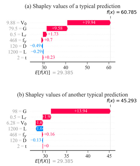
Figure 10.
Local explanation of a specimen.
6. Web Application
The results obtained in this study are valuable, but developing a user-friendly web application tool would promote GWO-XGB model adoption in engineering practice. The web application developed in this study uses seven input parameters to directly obtain the of CHS steel members under transverse impact loads. Notably, there should be no need for coding to display the results. This web application can also assist engineers in obtaining accurate and fast results, regardless of the complexity of the equations. Accordingly, using the web application can save time and effort to estimate the of CHS steel members under transverse impact load in the pre-design process. The web application can be accessed via the link https://sakat92-wf-wf-nfdrqz.streamlit.app/ (accessed on 1 May 2023).
7. Conclusions
This study develops several hybrid ML models, combining XGB and five metaheuristic optimization algorithms (PSO, GWO, MFO, JA, and MVO) to predict the of CHS steel members under transverse impact load. The following are the conclusions that can be drawn from the results of this study:
- Hybrid ML models generalize better than the default XGB model. Compared with the default XGB model, R2 increases (by 2.201%, 2.830%, 1.572%, 1.258%, and 2.201%), RMSE decreases (by 27.095%, 33.263%, 19.185%, 15.419%, and 28.413%), and MAE reduces (by 15.061%, 19.815%, 3.912%, 4.081%, and 9.466%) in the test set, respectively, in the PSO-XGB, GWO-XGB, MFO-XGB, JA-XGB, and MVO-XGB models.
- Among hybrid ML models, the GWO-XGB model predicts better than the others, with the highest R2 value (0.981), the lowest RMSE (2.835 mm), and the MAE (1.906 mm) value in the test set.
- The SHAP method shows that , , and are the most influential factors in prediction.
- A web application is developed to facilitate prediction. Users can quickly visualize the results using the GWO-XGB model, making it the best tool for promoting the practical application of the model.
Although the results in this study are great, the developed ML models are based on the limited database presented in Table 1. Thus, the database should be widened to enhance the performance of the ML model. Specifically, the findings of this study are focused on CHS steel members. Other types of members should be considered in future work.
Supplementary Materials
The following supporting information can be downloaded at: https://www.mdpi.com/article/10.3390/buildings13061384/s1.
Author Contributions
Conceptualization, S.H.M.; Methodology, S.H.M.; Software, D.H.N.; Validation, D.-K.T.; Investigation, D.H.N. and V.-L.T.; Data curation, D.H.N.; Writing—original draft, S.H.M.; Writing—review & editing, V.-L.T. and D.-K.T.; Visualization, V.-L.T.; Supervision, D.-K.T. All authors have read and agreed to the published version of the manuscript.
Funding
This research is funded by the Hanoi University of Civil Engineering (HUCE), Hanoi, Vietnam, under grant number 01-NNC-ĐHXDHN.
Institutional Review Board Statement
Not applicable.
Informed Consent Statement
Not applicable.
Data Availability Statement
Some or all data, models, or code that support the findings of this study are available from the corresponding author upon reasonable request.
Conflicts of Interest
The authors declare no potential conflict of interest with respect to the research, authorship, and/or publication of this article.
References
- Wardenier, J.; Packer, J.A.; Zhao, X.-L.; van der Vegte, G. Hollow Sections in Structural Applications; CIDECT: Geneva, Switzerland, 2010. [Google Scholar]
- Bambach, M.R. Validation of a general design procedure for the transverse impact capacity of steel columns. J. Constr. Steel Res. 2018, 150, 153–161. [Google Scholar] [CrossRef]
- Zhu, A.-Z.; Xu, W.; Gao, K.; Ge, H.-B.; Zhu, J.-H. Lateral impact response of rectangular hollow and partially concrete-filled steel tubular columns. Thin-Walled Struct. 2018, 130, 114–131. [Google Scholar] [CrossRef]
- Jones, N.; Birch, R. Low-velocity impact of pressurised pipelines. Int. J. Impact Eng. 2010, 37, 207–219. [Google Scholar] [CrossRef]
- Zhu, L.; Liu, Q.; Jones, N.; Chen, M. Experimental study on the deformation of fully clamped pipes under lateral impact. Int. J. Impact Eng. 2018, 111, 94–105. [Google Scholar] [CrossRef]
- Zhang, R.; Zhi, X.-D.; Fan, F. Plastic behavior of circular steel tubes subjected to low-velocity transverse impact. Int. J. Impact Eng. 2018, 114, 1–19. [Google Scholar] [CrossRef]
- Chen, F.L.; Yu, T.X. Influence of Axial Pre-Load on Plastic Failure of Beams Subjected to Transverse Dynamic Load. Key Eng. Mater. 2000, 177–180, 255–260. [Google Scholar] [CrossRef]
- Al-Thairy, H.; Wang, Y. A numerical study of the behaviour and failure modes of axially compressed steel columns subjected to transverse impact. Int. J. Impact Eng. 2011, 38, 732–744. [Google Scholar] [CrossRef]
- Temsah, Y.; Jahami, A.; Khatib, J.; Sonebi, M. Numerical analysis of a reinforced concrete beam under blast loading. MATEC Web Conf. 2018, 149, 02063. [Google Scholar] [CrossRef]
- Liu, J.; Jones, N. Experimental investigation of clamped beams struck transversely by a mass. Int. J. Impact Eng. 1987, 6, 303–335. [Google Scholar] [CrossRef]
- Jilin, Y.; Norman, J. Further experimental investigations on the failure of clamped beams under impact loads. Int. J. Solids Struct. 1991, 27, 1113–1137. [Google Scholar] [CrossRef]
- Yu, J.; Jones, N. Numerical simulation of a clamped beam under impact loading. Comput. Struct. 1989, 32, 281–293. [Google Scholar] [CrossRef]
- Yu, J.-L.; Jones, N. Numerical simulation of impact loaded steel beams and the failure criteria. Int. J. Solids Struct. 1997, 34, 3977–4004. [Google Scholar] [CrossRef]
- Mannan, M.N.; Ansari, R.; Abbas, H. Failure of aluminium beams under low velocity impact. Int. J. Impact Eng. 2008, 35, 1201–1212. [Google Scholar] [CrossRef]
- Bambach, M.R.; Jama, H.; Zhao, X.L.; Grzebieta, R. Hollow and concrete filled steel hollow sections under transverse impact loads. Eng. Struct. 2008, 30, 2859–2870. [Google Scholar] [CrossRef]
- Zeinoddini, M.; Parke, G.A.R.; Harding, J.E. Axially pre-loaded steel tubes subjected to lateral impacts: An experimental study. Int. J. Impact Eng. 2002, 27, 669–690. [Google Scholar] [CrossRef]
- Zeinoddini, M.; Harding, J.E.; Parke, G.A.R. Axially pre-loaded steel tubes subjected to lateral impacts (a numerical simulation). Int. J. Impact Eng. 2008, 35, 1267–1279. [Google Scholar] [CrossRef]
- American Association of State Highway and Transportation Officials. Bridge Design Specifications; American Association of State Highway and Transportation Officials: Washington, DC, USA, 2014. [Google Scholar]
- EN1991-1-7; Eurocode 1—Actions on Structures—Part 1-7: General Actions—Accidental Actions. European Committee for Standardisation: London, UK, 2010.
- Jones, N. A theoretical study of the dynamic plastic behavior of beams and plates with finite-deflections. Int. J. Solids Struct. 1971, 7, 1007–1029. [Google Scholar] [CrossRef]
- Symonds, P.S.; Jones, N. Impulsive loading of fully clamped beams with finite plastic deflections and strain-rate sensitivity. Int. J. Mech. Sci. 1972, 14, 49–69. [Google Scholar] [CrossRef]
- Jones, N. Plastic Failure of Ductile Beams Loaded Dynamically. J. Eng. Ind. 1976, 98, 131–136. [Google Scholar] [CrossRef]
- Jones, N.; Shen, W.Q. A Theoretical Study of the Lateral Impact of Fully Clamped Pipelines. Proc. Inst. Mech. Eng. Part E J. Process. Mech. Eng. 1992, 206, 129–146. [Google Scholar] [CrossRef]
- Shen, W.Q.; Shu, D.W. A theoretical analysis on the failure of unpressurized and pressurized pipelines. Proc. Inst. Mech. Eng. Part E J. Process. Mech. Eng. 2002, 216, 151–165. [Google Scholar] [CrossRef]
- Soares, C.G.; Søreide, T.H. Plastic Analysis of Laterally Loaded Circular Tubes. J. Struct. Eng. 1983, 109, 451–467. [Google Scholar] [CrossRef]
- Bambach, M.R. Design of hollow and concrete filled steel and stainless steel tubular columns for transverse impact loads. Thin-Walled Struct. 2011, 49, 1251–1260. [Google Scholar] [CrossRef]
- B. S. Institution. Eurocode 1: Part 1-7: General Actions-Accidental Actions; European Committee for Standardisation: London, UK, 2006. [Google Scholar]
- B.S. Institution. Safety of Machinery-Equipment for Power Driven Parking of Motor Vehicles-Safety and EMC Requirements for Design, Manufacturing, Erection and Commissioning Stages; iTeh, Inc.: Newark, DE, USA, 2003. [Google Scholar]
- Salehi, H.; Burgueño, R. Emerging artificial intelligence methods in structural engineering. Eng. Struct. 2018, 171, 170–189. [Google Scholar] [CrossRef]
- Thai, H.-T. Machine learning for structural engineering: A state-of-the-art review. Structures 2022, 38, 448–491. [Google Scholar] [CrossRef]
- Tran, V.-L.; Kim, J.-K. Innovative formulas for reinforcing bar bonding failure stress of tension lap splice using ANN and TLBO. Constr. Build. Mater. 2023, 369, 130500. [Google Scholar] [CrossRef]
- Tran, V.-L.; Nguyen, D.-D. Novel hybrid WOA-GBM model for patch loading resistance prediction of longitudinally stiffened steel plate girders. Thin-Walled Struct. 2022, 177, 109424. [Google Scholar] [CrossRef]
- Tran, V.-L.; Thai, D.-K.; Kim, S.-E. Application of ANN in predicting ACC of SCFST column. Compos. Struct. 2019, 228, 111332. [Google Scholar] [CrossRef]
- Esteghamati, M.Z.; Flint, M.M. Developing data-driven surrogate models for holistic performance-based assessment of mid-rise RC frame buildings at early design. Eng. Struct. 2021, 245, 112971. [Google Scholar] [CrossRef]
- Esteghamati, M.Z.; Flint, M.M. Do all roads lead to Rome? A comparison of knowledge-based, data-driven, and physics-based surrogate models for performance-based early design. Eng. Struct. 2023, 286, 116098. [Google Scholar] [CrossRef]
- Shehadeh, A.; Alshboul, O.; Al Mamlook, R.E.; Hamedat, O. Machine learning models for predicting the residual value of heavy construction equipment: An evaluation of modified decision tree, LightGBM, and XGBoost regression. Autom. Constr. 2021, 129, 103827. [Google Scholar] [CrossRef]
- Dong, Y.; Qiu, L.; Lu, C.; Song, L.; Ding, Z.; Yu, Y.; Chen, G. A data-driven model for predicting initial productivity of offshore directional well based on the physical constrained eXtreme gradient boosting (XGBoost) trees. J. Pet. Sci. Eng. 2022, 211, 110176. [Google Scholar] [CrossRef]
- Le, H.-A.; Le, D.-A.; Le, T.-T.; Le, H.-P.; Hoang, H.-G.T.; Nguyen, T.-A. An Extreme Gradient Boosting approach to estimate the shear strength of FRP reinforced concrete beams. Structures 2022, 45, 1307–1321. [Google Scholar] [CrossRef]
- Li, J.; An, X.; Li, Q.; Wang, C.; Yu, H.; Zhou, X.; Geng, Y.-A. Application of XGBoost algorithm in the optimization of pollutant concentration. Atmos. Res. 2022, 276, 106238. [Google Scholar] [CrossRef]
- Nguyen, N.-H.; Abellán-García, J.; Lee, S.; Garcia-Castano, E.; Vo, T.P. Efficient estimating compressive strength of ultra-high performance concrete using XGBoost model. J. Build. Eng. 2022, 52, 104302. [Google Scholar] [CrossRef]
- Tran, V.-L.; Kim, J.-K. Ensemble machine learning-based models for estimating the transfer length of strands in PSC beams. Expert Syst. Appl. 2023, 221, 119768. [Google Scholar] [CrossRef]
- Tran, V.L.; Ahmed, M.; Gohari, S. Prediction of the ultimate axial load of circular concrete-filled stainless steel tubular columns using machine learning approaches. Struct. Concr. 2023. [Google Scholar] [CrossRef]
- Degtyarev, V.V.; Naser, M.Z. Boosting machines for predicting shear strength of CFS channels with staggered web perforations. Structures 2021, 34, 3391–3403. [Google Scholar] [CrossRef]
- Ma, L.; Zhou, C.; Lee, D.; Zhang, J. Prediction of axial compressive capacity of CFRP-confined concrete-filled steel tubular short columns based on XGBoost algorithm. Eng. Struct. 2022, 260, 114239. [Google Scholar] [CrossRef]
- Nguyen, V.-Q.; Tran, V.-L.; Nguyen, D.-D.; Sadiq, S.; Park, D. Novel hybrid MFO-XGBoost model for predicting the racking ratio of the rectangular tunnels subjected to seismic loading. Transp. Geotech. 2022, 37, 100878. [Google Scholar] [CrossRef]
- Feng, D.-C.; Wang, W.-J.; Mangalathu, S.; Hu, G.; Wu, T. Implementing ensemble learning methods to predict the shear strength of RC deep beams with/without web reinforcements. Eng. Struct. 2021, 235, 111979. [Google Scholar] [CrossRef]
- Nguyen, H.D.; Truong, G.T.; Shin, M. Development of extreme gradient boosting model for prediction of punching shear resistance of r/c interior slabs. Eng. Struct. 2021, 235, 112067. [Google Scholar] [CrossRef]
- Rahman, J.; Ahmed, K.S.; Khan, N.I.; Islam, K.; Mangalathu, S. Data-driven shear strength prediction of steel fiber reinforced concrete beams using machine learning approach. Eng. Struct. 2021, 233, 111743. [Google Scholar] [CrossRef]
- Bakouregui, A.S.; Mohamed, H.M.; Yahia, A.; Benmokrane, B. Explainable extreme gradient boosting tree-based prediction of load-carrying capacity of FRP-RC columns. Eng. Struct. 2021, 245, 112836. [Google Scholar] [CrossRef]
- Azizi, M.; Shishehgarkhaneh, M.B.; Basiri, M. Optimum design of truss structures by Material Generation Algorithm with discrete variables. Decis. Anal. J. 2022, 3, 100043. [Google Scholar] [CrossRef]
- Daryan, A.S.; Salari, M.; Palizi, S.; Farhoudi, N. Size and layout optimum design of frames with steel plate shear walls by metaheuristic optimization algorithms. Structures 2023, 48, 657–668. [Google Scholar] [CrossRef]
- Azizi, M.; Aickelin, U.; Khorshidi, H.A.; Shishehgarkhaneh, M.B. Shape and size optimization of truss structures by Chaos game optimization considering frequency constraints. J. Adv. Res. 2022, 41, 89–100. [Google Scholar] [CrossRef]
- Jafari, M.; Salajegheh, E.; Salajegheh, J. Optimal design of truss structures using a hybrid method based on particle swarm optimizer and cultural algorithm. Structures 2021, 32, 391–405. [Google Scholar] [CrossRef]
- Alkayem, N.F.; Cao, M.; Shen, L.; Fu, R.; Šumarac, D. The combined social engineering particle swarm optimization for real-world engineering problems: A case study of model-based structural health monitoring. Appl. Soft Comput. 2022, 123, 108919. [Google Scholar] [CrossRef]
- Tran-Ngoc, H.; Khatir, S.; Ho-Khac, H.; De Roeck, G.; Bui-Tien, T.; Wahab, M.A. Efficient Artificial neural networks based on a hybrid metaheuristic optimization algorithm for damage detection in laminated composite structures. Compos. Struct. 2020, 262, 113339. [Google Scholar] [CrossRef]
- Sang-To, T.; Le-Minh, H.; Wahab, M.A.; Thanh, C.-L. A new metaheuristic algorithm: Shrimp and Goby association search algorithm and its application for damage identification in large-scale and complex structures. Adv. Eng. Softw. 2023, 176, 103363. [Google Scholar] [CrossRef]
- Kaveh, A. Advances in Metaheuristic Algorithms for Optimal Design of Structures; Springer International Publishing: Cham, Switzerland, 2021. [Google Scholar] [CrossRef]
- Li, E.; Zhou, J.; Shi, X.; Armaghani, D.J.; Yu, Z.; Chen, X.; Huang, P. Developing a hybrid model of salp swarm algorithm-based support vector machine to predict the strength of fiber-reinforced cemented paste backfill. Eng. Comput. 2020, 37, 3519–3540. [Google Scholar] [CrossRef]
- Qiu, Y.; Zhou, J.; Khandelwal, M.; Yang, H.; Yang, P.; Li, C. Performance evaluation of hybrid WOA-XGBoost, GWO-XGBoost and BO-XGBoost models to predict blast-induced ground vibration. Eng. Comput. 2021, 38, 4145–4162. [Google Scholar] [CrossRef]
- Zhou, J.; Qiu, Y.; Khandelwal, M.; Zhu, S.; Zhang, X. Developing a hybrid model of Jaya algorithm-based extreme gradient boosting machine to estimate blast-induced ground vibrations. Int. J. Rock Mech. Min. Sci. 2021, 145, 104856. [Google Scholar] [CrossRef]
- Zhou, J.; Qiu, Y.; Zhu, S.; Armaghani, D.J.; Khandelwal, M.; Mohamad, E.T. Estimation of the TBM advance rate under hard rock conditions using XGBoost and Bayesian optimization. Undergr. Space 2021, 6, 506–515. [Google Scholar] [CrossRef]
- Tran, V.-L.; Kim, J.-K. Revealing the nonlinear behavior of steel flush endplate connections using ANN-based hybrid models. J. Build. Eng. 2022, 57, 104878. [Google Scholar] [CrossRef]
- Jones, N.; Birch, S.E.; Birch, R.S.; Zhu, L.; Brown, M. An Experimental Study on the Lateral Impact of Fully Clamped Mild Steel Pipes. Proc. Inst. Mech. Eng. Part E J. Process. Mech. Eng. 1992, 206, 111–127. [Google Scholar] [CrossRef]
- Chen, K.; Shen, W.Q. Further experimental study on the failure of fully clamped steel pipes. Int. J. Impact Eng. 1998, 21, 177–202. [Google Scholar] [CrossRef]
- Jones, N.; Birch, R.S. Influence of Internal Pressure on the Impact Behavior of Steel Pipelines. J. Press. Vessel. Technol. 1996, 118, 464–471. [Google Scholar] [CrossRef]
- Li, Q.-F.; Song, Z.-M. High-performance concrete strength prediction based on ensemble learning. Constr. Build. Mater. 2022, 324, 126694. [Google Scholar] [CrossRef]
- Munir, M.J.; Kazmi, S.M.S.; Wu, Y.-F.; Lin, X.; Ahmad, M.R. Development of a novel compressive strength design equation for natural and recycled aggregate concrete through advanced computational modeling. J. Build. Eng. 2022, 55, 104690. [Google Scholar] [CrossRef]
- Chen, T.; Guestrin, C. XGBoost: A Scalable Tree Boosting System. In Proceedings of the KDD’16: 22nd ACM SIGKDD International Conference on Knowledge Discovery and Data Mining, San Francisco, CA, USA, 13–17 August 2016; Association for Computing Machinery: New York, NY, USA, 2016; pp. 785–794. [Google Scholar] [CrossRef]
- Friedman, J.H. Greedy function approximation: A gradient boosting machine. Ann. Stat. 2001, 29, 1189–1232. [Google Scholar] [CrossRef]
- Ding, Z.; Nguyen, H.; Bui, X.-N.; Zhou, J.; Moayedi, H. Computational Intelligence Model for Estimating Intensity of Blast-Induced Ground Vibration in a Mine Based on Imperialist Competitive and Extreme Gradient Boosting Algorithms. Nat. Resour. Res. 2020, 29, 751–769. [Google Scholar] [CrossRef]
- Zhang, W.; Zhang, R.; Wu, C.; Goh, A.T.; Wang, L. Assessment of basal heave stability for braced excavations in anisotropic clay using extreme gradient boosting and random forest regression. Undergr. Space 2022, 7, 233–241. [Google Scholar] [CrossRef]
- Zhang, W.; Wu, C.; Zhong, H.; Li, Y.; Wang, L. Prediction of undrained shear strength using extreme gradient boosting and random forest based on Bayesian optimization. Geosci. Front. 2021, 12, 469–477. [Google Scholar] [CrossRef]
- Kennedy, J.; Eberhart, R. Particle Swarm Optimization. In Proceedings of the ICNN’95—International Conference on Neural Networks, Perth, Australia, 27 November–1 December 1995; pp. 1942–1948. [Google Scholar] [CrossRef]
- Mirjalili, S.; Mirjalili, S.M.; Lewis, A. Grey Wolf Optimizer. Adv. Eng. Softw. 2014, 69, 46–61. [Google Scholar] [CrossRef]
- Mirjalili, S. Moth-flame optimization algorithm: A novel nature-inspired heuristic paradigm. Knowl. Based Syst. 2015, 89, 228–249. [Google Scholar] [CrossRef]
- Rao, R.V. Jaya: A simple and new optimization algorithm for solving constrained and unconstrained optimization problems. Int. J. Ind. Eng. Comput. 2016, 7, 19–34. [Google Scholar] [CrossRef]
- Mirjalili, S.; Mirjalili, S.M.; Hatamlou, A. Multi-Verse Optimizer: A nature-inspired algorithm for global optimization. Neural Comput. Appl. 2016, 27, 495–513. [Google Scholar] [CrossRef]
- Kaveh, A.; Eslamlou, A.D.; Moghani, R.M. Shear Strength Prediction of FRP-reinforced Concrete Beams Using an Extreme Gradient Boosting Framework. Period. Polytech. Civ. Eng. 2021, 66, 18–29. [Google Scholar] [CrossRef]
- Nguyen, Q.H.; Ly, H.-B.; Ho, L.S.; Al-Ansari, N.; Van Le, H.; Tran, V.Q.; Prakash, I.; Pham, B.T. Influence of Data Splitting on Performance of Machine Learning Models in Prediction of Shear Strength of Soil. Math. Probl. Eng. 2021, 2021, 4832864. [Google Scholar] [CrossRef]
- Qi, C.; Guo, L.; Ly, H.-B.; Van Le, H.; Pham, B.T. Improving pressure drops estimation of fresh cemented paste backfill slurry using a hybrid machine learning method. Miner. Eng. 2021, 163, 106790. [Google Scholar] [CrossRef]
- Tran, V.-L.; Jang, Y.; Kim, S.E. Improving the axial compression capacity prediction of elliptical CFST columns using a hybrid ANN-IP model. Steel Compos. Struct. 2021, 39, 319–335. [Google Scholar] [CrossRef]
- Tran, V.-L.; Kim, S.-E. Rapid prediction of the ultimate moment of flush endplate connections at elevated temperatures through an artificial neural network. Expert Syst. Appl. 2022, 206, 117759. [Google Scholar] [CrossRef]
- Tran, V.-L.; Kim, S.-E. A practical ANN model for predicting the PSS of two-way reinforced concrete slabs. Eng. Comput. 2020, 37, 2303–2327. [Google Scholar] [CrossRef]
- Lundberg, S.M.; Lee, S.I. A unified approach to interpreting model predictions. Adv. Neural Inf. Process. Syst. 2017, 30, 4766–4775. [Google Scholar]
Disclaimer/Publisher’s Note: The statements, opinions and data contained in all publications are solely those of the individual author(s) and contributor(s) and not of MDPI and/or the editor(s). MDPI and/or the editor(s) disclaim responsibility for any injury to people or property resulting from any ideas, methods, instructions or products referred to in the content. |
© 2023 by the authors. Licensee MDPI, Basel, Switzerland. This article is an open access article distributed under the terms and conditions of the Creative Commons Attribution (CC BY) license (https://creativecommons.org/licenses/by/4.0/).