Abstract
Accurate prediction of the prestressed steel amount is essential for a concrete-road bridge’s successful design, construction, and long-term performance. Predicting the amount of steel required can help optimize the design and construction process, and also help project managers and engineers estimate the overall cost of the project more accurately. The prediction model was developed using data from 74 constructed bridges along Serbia’s Corridor X. The study examined operationally applicable models that do not require indepth modeling expertise to be used in practice. Neural networks (NN) models based on regression trees (RT) and genetic programming (GP) models were analyzed. In this work, for the first time, the method of multicriteria compromise ranking was applied to find the optimal model for the prediction of prestressed steel in prestressed concrete bridges. The optival model based on GP was determined using the VIKOR method of multicriteria optimization; the accuracy of which is expressed through the MAPE criterion is 9.16%. A significant average share of 46.11% of the costs related to steelworks, in relation to the total costs, indicates that the model developed in the paper can also be used for the implicit estimation of construction costs.
1. Introduction
The development of a society and the state is highly dependent on the development of traffic and the state of the traffic infrastructure. The traffic infrastructure consists of many bridges, viaducts, culverts, and other facilities and is constantly expanding. In the entire past millennium to the 20th century, fewer bridges were built than now in one decade [1]. More than two million bridges are currently in use throughout the world [1]. Over 80% of the bridges built are concrete-girder bridges, with a significant share of prestressed concrete bridges. Many construction activities accompany the construction of bridges on roads, significant earthworks, geotechnical works, construction of the bridge structure itself, works on signaling, lighting, and construction of culverts and accompanying facilities.
A subset of artificial intelligence known as machine learning (ML) enables computer systems to learn from their past performance and advance accordingly. It entails analyzing and discovering patterns in data using statistical models and algorithms, followed by utilizing these patterns to create forecasts or conclusions regarding brand-new data. In numerous types of research in construction, it is applied to the random forest, AdaBoost, gradient boost regression trees, support vector regression, extreme gradient boosting, and ANN algorithms. Some successful implementations of these algorithms in predicting the behavior of elements in construction are listed in the works of Tang et al. (2022), Feng et al. (2023), and Zhao et al. (2023) [2,3,4].
A sufficiently accurate estimation of resources is essential when analyzing various technical solutions for bridges when detailed data on designed bridges are unavailable. In addition, the availability of information about the resources needed for the construction of bridges in the initial stages of the project enables the entire project to be seen more comprehensively to provide initial construction cost estimates for funding acquisition purposes and also from the aspect of maintenance through the analysis of the whole life cycle of the project. Recent thorough reviews of the literature and content evaluations of construction cost prediction models by Tayefeh Hashemi et al. (2020) and Antoniou et al. (2023) have shown that numerous models offering cost estimates and/or material consumption estimates at various design stages have been provided by researchers, mostly for buildings, but also for power generation or network construction, road construction, rail and road tunnels, and bridges [5,6].
One of the most detailed comparative studies related to the consumption of resources in bridge construction was done in 2001 by Flyvbjert et al. [4]. The total value of the analyzed projects in North America and Europe was over USD 90 billion. The results indicated that the average percentage error in cost estimation for bridges and tunnels is 33.8%, while the total average error for all analyzed projects is 27.6%. One of the important conclusions is the subjectivity in the assessment of resources in the construction of construction facilities [7].
An analysis of the consumption of resources, concrete, prestressed steel, and reinforcing steel, and equations for their assessment in the construction of prestressed bridges are provided by Men in 1991 in the book Prestressed Concrete Bridges [8]. The analysis is based on records of resource consumption during the construction of 19 prestressed concrete bridges in Switzerland. The cost of building bridges, as well as the consumption of resources during construction, is given as a function of the variable defined as the geometrical average-span length.
In 2001 Marcous et al. [9] worked on a preliminary quantity estimate of highway bridges using artificial-intelligence methods. On the basis of 22 prestressed concrete bridges across the Nile River in Egypt, artificial neural-network models were developed. In terms of testing the accuracy of the model, cross validation was used. As a result, it was found that the error of the created model in estimating the weight of prestressed steel is 11.5%.
The Egnatia Motorway, a 680 km long modern highway that serves five ports and six airports and connects the major cities of Northern Greece, is one of the largest civil engineering projects ever undertaken in Europe. A number of Greek researchers have used data from the Egnatia Motorway’s bridges to develop their models for estimating bridge material consumption and construction costs. It is one of the original fourteen priority projects of the European Union and constitutes part of the Trans-European Network for Transport [10].
More specifically, Fragkakis et al., in 2011 [11], worked on a parametric model for estimating resources in the construction of concrete-bridge foundations. Their database included complete data on 78 structures and 157 pier foundations. The coefficient of determination exceeds 77% in all prediction models. Antoniou et al. [12,13] worked on a model for estimating highway bridge-underpass costs and material consumption. The research was based on data from 28 closed-box sections and six frame underpasses from the Egnatia Motorway and the E65 Motorway in Greece. Their first study [12] provided consumption values of reinforcing steel per m3 of used concrete and the so-called theoretical volume of the structure. This new variable is described as the product of the length, width, and overhead clearance height of the local road that needs to be reconfigured to pass underneath the freeway. The same research team proceeded to develop more accurate linear regression models for forecasting the costs of underpass bridges, concrete consumption, and reinforcing steel consumption, depending on two input variables, i.e., the bridge surface area and the theoretical volume. As a result, satisfactory values of the coefficient of determination for cost estimation, consumption of concrete, and consumption of reinforcing steel of 0.80, 0.85, and 0.70, respectively, were obtained [12,13]. Similarly, Antoniou et al. [14] provided an analytical formulation for early cost estimation and material consumption of road overpass bridges in 2016. The database included data on 57 completed overpasses on the Egnatia Motorway. The research defined linear models for cost estimation, reinforcing steel consumption, and prestressing steel consumption. In the model for forecasting the consumption of prestressing steel, linear models are given for assessment depending on the deck surface area as an input variable and depending on the theoretical volume of the bridge, whose coefficient of determination value is 0.85 and 0.73, respectively. In this case the theoretical volume of the bridge is defined as the deck length multiplied by its width multiplied by the average pier height. In order to promote the use of prefabrication in the design and construction of highway concrete bridges in countries with nonwell-established relevant standards, Antoniou and Marinelli used multilinear regression analysis [15]. They proposed a set of standard precast extended I beams suitable for use in the majority of the common motorway-bridge models. The data of 2284 total beams from 109 bridges built along the Egnatia Motorway and two of its perpendicular axes [15] form the basis of the suggested set of standard beams.
Marinelli et al. [16] in 2015 worked on researching the application of artificial neural networks for nonparametric bill-of-quantities estimation of concrete road bridges. The data used to develop the model consists of 68 motorway bridges constructed in Greece between 1996 and 2008. A neural network model was used for forward signal propagation, and three output variables were forecast: the volume of concrete, the weight of reinforcing steel, and the weight of prestressed steel. The model’s accuracy expressed through the MAPE criterion was 11.48% for precast beams, 13.94% for cast in situ, and 16.12% for the cantilever construction method.
Kovačević et al. created a number of models in 2021 [17] for estimating the cost of bridges made of reinforced concrete (RC) and prestressed concrete (PC). The characteristics of the project and the tender documents were included in the database for the 181 bridges in Serbia’s Corridor X that were finished. The research’s best option was a model based on Gaussian random processes, and it had an accuracy of 10.86% by the MAPE criterion.
Kovačević and Bulajić carried out a study in 2022 [18] to predict the consumption of prestressed steel used in the construction of PC bridges using machine-learning (ML) techniques. In Serbia’s Corridor X, the database contained data on 75 completed prestressed bridges. According to the specified criterion MAPE, the model’s accuracy in determining the prestressed steel consumption per square meter of the bridge superstructure was 6.55%.
The application of artificial neural-network models (ANNs), models based on regression trees (RTs), models based on support-vector machines (SVM), and Gaussian processes regression (GPR) are all taken into consideration by Kovačević et al. [19] in order to estimate the concrete consumption of bridges based on a database for the 181 bridges in Serbia’s Corridor X in 2022. The most precise model, with a MAPE of 11.64%, is produced by employing GPR in combination with ARD’s covariance function, according to the study. Also, the application of the GPR ARD covariance function makes it possible to see the importance of each input variable to the model’s accuracy.
The development of a model for forecasting the amount of steel in this research is significant for science for several reasons. The prediction of the prestressed steel amount for a concrete road bridge is important for cost estimation, structural integrity, and the efficiency of the design and construction processes. The amount of prestressed steel used in a bridge directly affects the cost of construction. Accurately predicting the amount of steel required can help project managers and engineers estimate the overall cost of the project more accurately.
In this research, the hypothesis is that it is possible to define a model for forecasting the amount of prestressing steel using machine learning methods that will be accurate and transparent enough for practical application and where the amount of prestressing steel can be obtained based on a narrow set of model input variables. The RMSE, MAE, R, and MAPE criteria were defined for evaluating the model, while an effort was made to find a model with less complexity. In addition, the aim was to find a model that would, to the greatest extent, simultaneously satisfy all of the set criteria but at the same time is not particularly bad according to any individual criterion from the defined criteria.
In addition, to the author’s knowledge, the method for finding the optimal compromise solution VIKOR was applied for the first time for forecasting the amount of prestressing steel. In this way, implementing the VIKOR method, within the set of potential alternatives that are represented by individual models that have different accuracy according to the selected criteria, there is a solution that satisfies all criteria well overall but is the least bad according to individual criteria.
2. Methods
In order to calculate the amount of prestressing steel used in the construction of prestressed concrete road bridges, different ML approaches are presented and analyzed in this study. The use of artificial neural networks, models based on the regression trees, and multigene genetic programming (MGGP) models were examined.
2.1. Multilayer Perceptron (MLP) Neural-Network Models
Multilayer perceptron (MLP) neural networks are a type of feed-forward artificial neural network that is commonly used for supervised-learning tasks. They are called “multi-layer” since they contain one or more hidden layers in addition to the input and output layers. Due to their ease of implementation and ability to simulate a variety of complex functions, MLP neural networks are widely employed.
The basic structural element (Figure 1) of neural networks is a neuron. The neuron model consists of the following elements [20].
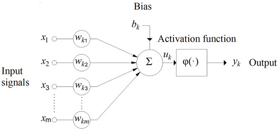
Figure 1.
Artificial-neuron model [20].
- A collection of synapses that have corresponding weight values;
- Summarizing part, where inputs multiplied by appropriate weights are added;
- Appropriate activation function that restricts the neuron’s output.
An artificial neuron consists of a group of weight coefficients that enter the body of a neuron, known as the node or unit, and a set of weights. Weights are connections with other neurons from the previous layer that then add up, and in the end, the bias value is added, which is independent of the other weights and serves to correct the sum. The following Equations (1) and (2) can mathematically explain this:
where are the corresponding input values of individual variables, and are the corresponding weights for neurons k and bk, the calculated bias.
A feed-forward neural network called a multilayer perceptron (Figure 2) consists of individual neurons grouped in at least three layers:
- Data enters the network at the input layer;
- All calculations using the data, weights, and biases are performed in the hidden layer;
- The output layer from which outcomes are obtained.

Figure 2.
Multilayer perceptron (MLP) neural network [20].
If the MLP architecture with the property of universal approximator is used, the determination of the network structure is reduced to the determination of the number of neurons of the hidden layer since the number of input neurons is determined by the dimensions of the input vector and the number of output neurons is determined by the dimension of the output vector.
An MLP model with one hidden layer whose neurons have a tangent hyperbolic sigmoidal activation function, while the neurons of the output layer have a linear activation function, can approximate an arbitrary multidimensional function for a given dataset when there are a sufficient number of neurons in the hidden layer [17].
There are numerous recommendations regarding the approximate number of neurons in the hidden layer, some of which are listed in Table 1.

Table 1.
Recommendations for the number of neurons in the hidden layer of a neural network.
Where the is number of inputs, is number of samples, and is number of outputs.
In this paper, the upper limit of the number of neurons was adopted, and then different architectures of neural networks were examined, starting with one neuron in the hidden layer and finally with the number of neurons equal to the upper limit obtained by the expression in row 6 in Table 1.
2.2. Regression-Trees (RTs) Models
Regression trees (RTs) are a straightforward and understandable machine-learning model that may be used for regression and classification [20]. In each tree node, except for the leaves, the corresponding condition is examined. Whether the condition is met or not, one or the other branch of the tree goes to the next node. An example of a decision tree is given in Figure 3. For the corresponding input quantity, that is, the instance (a vector or matrix) of the problem under consideration and for which a prediction needs to be made, the corresponding condition at the root of the tree is first examined. Then, depending on the result, the instance follows the branch that corresponds to that result to the next node and repeats the process until it reaches the terminal leaf, whose value indicates the requested prediction. All instances of space initially belong to the same set, and then space is gradually split up into subsets.
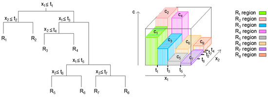
Figure 3.
Example of segmenting variable spaces into regions (left), the creation of a 3D regression surface (right) [20].
The split variable j and split point value s, which serve as the location at which the division of space will be carried out, must be determined. Its value corresponds to the minimum value of the expression (3) that can be determined by examining all of the input variables in the model [26,27]:
where = and =
After identifying the split variable j and the best-split point s, the process is maintained by further splitting these regions until a specific stop criterion is satisfied. This approach represents the so-called greedy approach since it only considers what is optimal in the current iteration, not considering whether that decision is also globally optimal [20,26,27].
According to the implemented binary recursive segmentation (Figure 3 (left)), each step involves splitting the input space into two parts and repeating the segmentation process. The resulting areas or regions should not overlap and encompass the whole space of predictors or input variables. In binary recursive partitioning, the output is characterized by the mean value in each of the two areas that make up the input space.
The Figure 3 shows the mean values for regions denoted with (Figure 3 (right)). Regions are defined using specific values , which represent the obtained optimal values for split point values s for split variables and .
In this way, instead of one linear model for the entire domain of the considered problem, the domain is fragmented into a larger number of subdomains in which the corresponding linear model is implemented.
Deep regression trees are typically prone to overfitting since, by applying a large number of conditions, such trees can describe even irrelevant specificities of the data on which they were trained. Shallow trees typically have the problem of underfitting. Based on this, it can be concluded that the depth of the tree represents a regularization hyperparameter. The good side of decision trees is their interpretability. If the tree is small, its conditions clearly indicate the basis on which it makes decisions.
Moreover, each path through the decision tree from root to leaf can be seen as a single if–then rule, in which the condition represents the conjunction of all conditional outcomes along the path, while the final decision is the numerical value in the terminal leaf. Another advantage of using regression trees is that regression trees can combine categorical and continuous attributes.
2.3. Multigene Genetic-Programming (MGGP) Models
Genetic programming (GP) is a machine-learning method based on evolutionary principles applied to mathematical models of the problem under consideration [28]. The basic idea lies in the evolutionary principle that the biological individual best adapted to the environment survives. Analogous to that approach, individual prediction models can be considered biological individuals. The models that provide the most accurate forecast for the output-model variable can be considered the most adapted and survive and go into the next generation with other adapted models.
With the MGGP method [29,30,31,32], individuals are first created, making up the initial population (Figure 4). Then, each individual model is represented by one or more trees. The tree model is formed in the first iteration as a random selection of mathematical functions, constants, and model variables. Each tree represents one gene. Trees end with terminal nodes that are either model input variables or constants, while all other nodes are called functional nodes.
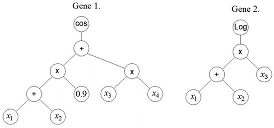
Figure 4.
An example of an MGGP model that has two genes [17].
One prediction MGGP model consists of one or more trees or genes. After the formation of the initial population of a specific size, the models that are the most adapted, which in MGGP modeling means the models whose prediction differs the least from the target value, are selected. Those best models are then used to create the next population of models through crossover, mutation, and direct copying of individuals of the previous generation. In practical implementation, the selection is made, probabilistically based on the model’s fitness value and/or complexity. The complexity of the model is based on the number of nodes and subtrees that can be formed from the given tree, which represents the so-called expressional complexity of the model.
A gene can either be replaced entirely during the crossover or partially changed [29,30,31,32]. If it is assumed that the individual model marked with (4) contains the following genes [ and if it is assumed that the other individual model marked with (5) contains the following genes . Let us indicate by <> the genes that are randomly selected in both models with two cross sections:
The bolded portions of the model or entire genes covered by random cross sections are exchanged in the offspring (6) and offspring (7), which represents the so-called high-level crossover procedure [20].
Crossover is also implemented at the level of one gene (low-level crossover), where the structure of a part of the gene changes (Figure 5a,b). However, only part of the gene may be exchanged (that is, only part of the tree is exchanged).
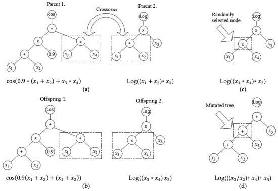
Figure 5.
Crossover and mutation operation in MGGP: (a) random selection of parent tree nodes; (b) exchange of parents’ genetic material; (c) random node selection in tree mutation; and (d) mutation of a randomly selected part of a tree [20].
It is also possible to mutate at the level of a single gene in addition to crossover (Figure 5c,d). A mutation involves the random selection of one gene and one node within it. The relevant mutation is then carried out, adding a subtree that was randomly generated at the location of the chosen node. A specified number of iterations are made using the aforementioned processes.
The model obtained this way is pseudolinear since it represents a linear combination of nonlinear individual models in the form of a tree.
Mathematically, a multigene regression model can be represented by the following Equation (8):
where is the bias term, is the ith scaling parameter, is the ( vector of outputs from the ith tree (gene), and whose structure is represented by Figure 6.
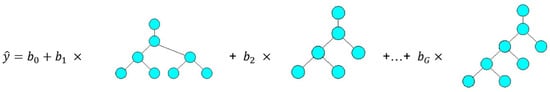
Figure 6.
The general structure of the MGGP model [20].
With G, it is denoted the gene-response matrix, or … ], whose dimensionality is and b is a vector of the coefficients is the dimensionality . Taking into account the above, the multigene regression model can be written in the following Equation (9):
From the training data, the vector is the least-squares estimate and it can be calculated using the following Equation (10):
Regular tournament selection, which solely employs RMSE or Pareto tournament, is used to choose individuals for breeding. Each individual in a Pareto tournament is chosen probabilistically based on their RMSE (fitness) score and expressional complexity. The procedure is successively repeated until a certain stopping criterion is reached.
2.4. Method for Multicriteria Compromise Ranking VIKOR
Very often, to solve various optimization problems, it is necessary to choose a solution that is evaluated based on a large number of criteria. Multicriteria decision-making (MCDM) approaches are used when selecting the best alternative from a list of potential alternatives due to their capacity to consider various and frequently conflicting criteria to create rankings of alternatives. Many different MCDMs have been adopted for decision making in the construction industry [33,34]. One of the ways to solve the problem is the VIKOR compromise programming method, which ranks the alternatives in such a way that they propose an alternative that ensures the maximum satisfaction of the majority of the defined criteria and, at the same time, is not particularly bad according to specific criteria [35,36,37,38,39]. It can be said that the proposed compromise solution is a compromise that satisfies both the majority and the minority criteria at the same time.
Compromise programming proposes establishing a reduced set of solutions to the problem of multicriteria optimization by employing the ideal point as a reference point in the space of criterion functions.
Suppose that there is an optimal solution , ie. , according to the i-th criterion (11):
where represents the maximum if that criterion function represents something that is “good” that it is wanted to be maximized, such as profit, benefit, etc., or minimum if it represents something that is “bad” that it is wanted to be minimized, such as cost, something that is harmful, etc.
The vector = (, where n is the total number of criterion functions, is the ideal solution to the problem of multicriteria decision making. In practice, it is rare that a potential solution is simultaneously optimal according to all of the individual criteria , .
In real situations, it is necessary to find a solution closest to the ideal based on some adopted measure of distance. Therefore, in the VIKOR method, the measure of the distance from an ideal point defined by Equation (12) [33,34,35,36,37] is used:
This metric represents the distance between the ideal point and point ) in the space of criterion functions. In order to emphasize the dependence on the parameter p, the metric will be denoted by ).
The solution which achieves the minimum of the function , is called the compromise solution of the multicriteria optimization problem with the parameter p [35,36,37,38,39].
The function for has the following form (13):
When the value of the parameter p tends to infinity, the problem of the distance from the ideal point is reduced to the mini–max problem.
In the case of compromise optimization, in the general case, it is necessary to determine the sequence for a particular set of alternatives According to the defined criteria .
The distance of some alternative , concerning the ideal point in relation to all defined criteria (the criteria are considered in summary), is measured by the measure , which is defined by the following Equation (14):
where represents the weight attached to some criterion ; represents the value of i-th criterion function for the alternative ; represents the best value according to criterion ; and represents the worst value according to criterion ().
The distance of some alternative , concerning the ideal point to certain individual criteria, is defined through the measure , which is defined by the following Equation (15):
Using the defined measures and , the initially defined problem of finding the optimal solution concerning the defined criteria , , is reduced to a two-criteria problem of optimizing the distance from the ideal point.
The ideal alternative in the new two-criteria problem has the following goodness-measure values (16), (17):
The definitive measure of the optimality of an alternative is determined by the value , which represents the superposition of measures and , i.e., the balance between the fact that the better alternatives better meet the majority of criteria and have a minimal deviation from individual criteria, is determined by the Equation (18):
where is the weight of decision-making strategy satisfying the majority of criteria, is the weight of decision-making strategy taking into account the individual criterion, the distance values of individual alternatives are normalized in relation to measures and , i.e., , and . If both strategies have the same weight, then .
According to [35,36,37,38,39], the VIKOR approach only proposes the alternative that is in the first position on the compromise ranking list for as a multicriteria optimal alternative (for specified weights ) if it also has:
- “sufficient advantage” over the alternative from the next position (condition );
- “sufficiently firm” first position with weight change (condition ).
Alternative has a sufficient advantage for over the following from the ranking list if (19):
where is the “priority threshold” = min (0.25;1/(J − 1)), and J represents the total number of problem alternatives.
3. Dataset
This research analyzed the consumption of prestressing steel in prestressed concrete bridges (prefabricated or cast onsite). In order to create an appropriate model for assessment, it was necessary to create an appropriate database on prestressed bridges, for which data was collected on realized prestressed concrete bridges on Corridor X in Serbia. In addition, project and contract documentation was collected for 74 completed bridges on the highway and the connecting roads to the highway (Figure 7).
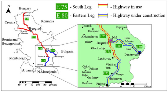
Figure 7.
Eastern and southern legs of Corridor X in Serbia [17].
Most research uses a modified span variable. In this research, variables were introduced that take into account the maximum individual span, the average span, and the total length span of the bridge since it is very important for the model whether the bridge is made of a larger number of smaller spans or a smaller number of larger spans. In addition, sometimes, not all spans on the same bridge are the same. Since, in the case of bridges that have more spans, where a certain span can be slightly larger than the other spans (e.g., due to the river that the bridge spans), a variable describing the maximum span was introduced.
In addition, the dataset included bridges on the highway itself, but also a certain number of access bridges, so a variable was introduced that contains information about the width of the road. The variable that contains information about the width of the road implicitly contains information about the useful load. The bridges that were analyzed were located in a narrow geographical area, and there were no differences in terms of load, so the load was not treated as a separate variable.
The data was divided so that 70% of the total data was assigned to the training set, and the remaining 30% of the data that the model did not see was used for testing the model. When dividing the data, it was taken into account that these two sets of data should have similar statistical characteristics.
The data was divided by mixing the entire set using the integrated randperm Matlab function several times and then randomly separating the training and test set from it in the specified percentage while controlling the statistical indicators of the training and test set, which should be, ideally, in the case of the same, that is, in the practical research of similar values. A total of 52 datasets were used for model training. The remaining data from 22 datasets were not submitted to the model and were used for model evaluation.
For the input variables for the forecast model of prestressing steel per of the bridge superstructure, the following were taken: —maximum individual bridge span (MIBS), —average bridge span (ABS), —total bridge span (TBS) length, —bridge width (BW).
Based on project documents, the dependent variable PS, being the mass in kg of prestressed steel per of the bridge superstructure, is calculated. The statistical characteristics of the model variables are given in Table 2. The mechanical characteristics of the prestressing steel are given in Table 3.
Table 2.
Mean, minimum, and maximum values of variables in the model used to estimate the prestressed steel consumption per of the bridge superstructure.
Table 3.
Geometrical and mechanical rope characteristics [18].
By analyzing the correlation matrices of the considered variables of the model, it can be observed that there is a significant intercorrelation of the variables of the model. Significant intercorrelation of model variables significantly reduces the accuracy of linear regression models, and nonlinear machine-learning models are particularly suitable for modeling in these cases.
In the specific case, all the variables related to the span are correlated (MIBS, ABS, and TBS) by the amount of prestressing steel as an output variable. However, the variable bridge width (BW), which has a low correlation with the value (R = 0.08) with the output variable, is correlated with other input variables. The application of machine-learning methods is particularly suitable in such cases of synergistic effects of individual input variables.
Data related to the consumption of prestressing steel is a good indicator of the total costs. In the formed database of 74 bridges, the calculated share of steel works in the total costs was 46.11%, while the share of concrete works was 40.66%. A model that would focus on the prediction of the amount of steel could also be used for implicit cost estimation.
Histograms of model variables and mutual correlations with the correlation coefficient values are given in Figure 8. From Figure 8, it is noticeable that there is a significant intercorrelation between most of the input variables of the model.
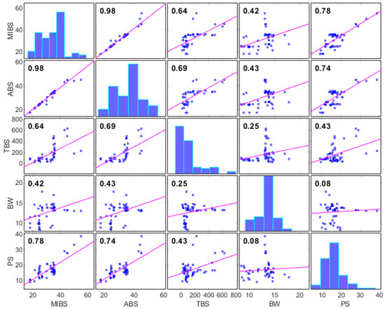
Figure 8.
Correlation matrix of model variables.
In Table 3, the mechanical characteristics of the prestressed steel ropes are listed for the reason that the limitation of the developed model is that the amount of steel obtained by prediction refers to the prestressed steel of the given characteristics.
Criteria for Assessing Model Accuracy
In the research, all models were trained and tested under identical conditions. When determining the optimal model, the accuracy of the model according to the criteria RMSE, MAE, R, and MAPE was taken into account, though the complexity of the model was also taken into account. The applied systemic approach to modeling is given in Figure 9. The RMSE and MAE criteria are absolute criteria of model accuracy expressed in the same unit as the variable that is being modeled. MAPE and R criteria are relative criteria of model accuracy and have no unit.
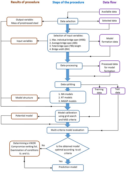
Figure 9.
Systemic approach applied in research.
The RMSE criterion is defined by Equation (20) and is characterized by the fact that deviations from the target value are first squared, then averaged, and then their square root is found. With such a calculation, a greater emphasis on greater deviations is given.
where is the target value, is the modeled output, and N is the number of samples.
The MAE is used to estimate the model’s mean absolute error and practically all deviations have the same weight. It is defined by the following Equation (21):
The R coefficient, is a relative criterion for the evaluation of the model’s accuracy. It is defined in dimensionless form by the following Equation (22):
where is the predicted mean and is the mean target value.
The mean absolute percentage error (MAPE) is a measure of prediction accuracy calculated in dimensionless form. The accuracy is expressed as a ratio determined by the following Equation (23):
When determining the optimal solution, the VIKOR method of multicriteria compromise ranking of alternatives was used to obtain a solution or model that will satisfy the majority of criteria, but will not be significantly bad, according to any defined individual criteria. In addition, the complexity of the model was taken as a criterion.
4. Results
With the applied methods depending on the method, a different data-preparation procedure was applied. In the method of artificial neural networks, linear scaling in the interval [0, 1] was applied so that all of the variables were equal during model training and then rescaled, and an accuracy assessment was performed after the output variables were rescaled. No scaling was applied to regression tree models and models based on genetic programming.
The MLP neural network has a fixed number of neurons in the input and output layers, with four and one neurons, respectively. However, the number of neurons in the hidden layer was determined through experimentation and was limited to a maximum of nine neurons based on expression in row six in Table 1.
For determining the optimal number of neurons in the hidden layer, the network was trained multiple times with different numbers of neurons in the hidden layer ranging from one to nine, as illustrated in Figure 10. The adopted limit of nine neurons is large enough to satisfy all the recommendations indicated by the expressions in Table 1. By analyzing Figure 10, it can be seen that the thus-adopted range for the number of neurons is satisfactory and, within that range, the accuracy functions RMSE, MAE, and MAPE have minima, while R achieves maximum. The results of the training indicate that the best number of neurons in the hidden layer is four, which was determined by evaluating the network’s performance using four quality criteria: RMSE, MAE, R and MAPE, as shown in Figure 10.
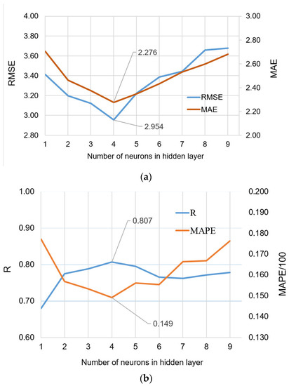
Figure 10.
Comparison of the accuracy criteria for MLP-ANNs with different numbers of neurons in the hidden layer: (a) RMSE and MAE; and (b) R and MAPE.
All models were trained within the Matlab program with default parameter settings. The LM algorithm was used.
The regression-tree model is built using a recursive binary-splitting process. Starting from the root node, the predictor variable that best separates the data into two subsets is selected using a split criterion mean-squared error (MSE). This process is repeated for each subset until a stopping criterion is reached. The splitting process continues until a set of leaf nodes is reached that provides predictions of the dependent variable. This research implements a minimum number of observations per node as the stopping criterion.
The performance of the regression tree can be improved by tuning the hyperparameters, such as the maximum tree depth and the minimum number of observations per node. This involves trying different values of the hyperparameters and evaluating the performance of the tree on the testing set. The goal is to find the optimal hyperparameters set that provides the best predictions.
In this research, the RT model examined different values of the minimum amount of data per parent node ranging from 1 to 10 and the minimum amount of data per terminal leaf from 1 to 10. All the models thus obtained were evaluated in terms of the defined accuracy criteria RMSE, MAE, R, and MAPE on a defined test set of subdata.
It was found that the optimal model with a min parent size equal to four and a minimum amount of data per terminal sheet is two. The structure of the regression table is given in Figure 11.
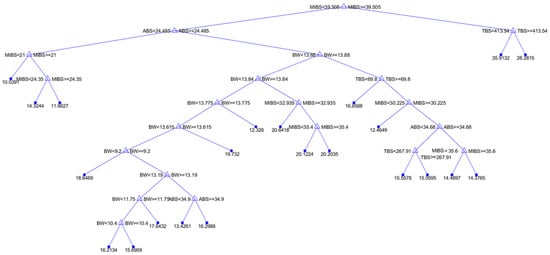
Figure 11.
Graphic representation of the optimal regression tree model.
With the MGGP model, the first population of random trees is generated to start the evolutionary process. In all models, a population of 1000 randomly generated trees was initially formed using a functional set composed of selected mathematical operators and randomly selected ephemeral random constant (ERC) values (Table 4). Within the MGGP model, the selection of the appropriate parameters in terms of crossover probability, mutation probability, and probability of the Pareto tournament, which determines the transfer of individuals to the next generation, is of crucial importance for creating the model. The ERC probability, which determines the probability of the appearance of certain values of constants from the range [−10, 10] in terminal leafs, is set to the value of 0.1, and the tournament size is set to the smallest value of two, which prevents premature convergence and ensures a greater diversity of individuals. The values for the number of genes were adopted in accordance with the recommendations of the authors of the GPTIPS 2.0 software with the maximum value of five, while the optimal depth of the trees was investigated experimentally.
Table 4.
Setting parameters for MGGP models.
Each tree in the population is then evaluated simultaneously based on fitness expressed through RMSE and expressional complexity. The fittest individuals from the population are selected to be parents for the next generation. The selected parents are then combined through genetic operators such as crossover and mutation to produce offspring for the next generation, and a certain percentage of trees (0.05% of the population) went directly to the next generation.
The offspring replace the least-fit individuals in the population to create the next generation. The evolutionary process is continued until a stopping criterion is met, such as a maximum number of generations or a desired level of fitness. The complexity of the model was examined using the MGGP approach using various values of the number of genes and various tree depths.
In this research, the maximum number of generations was limited to 100, and the procedure was repeated ten times for each gene structure with a defined maximum depth of the tree, and the models were combined. Models with one to five genes whose tree depth varied from one to six were tested. A total of 30,000,000 MGGP models were tested.
In order to single out the optimal models, a graphic representation of the population of models obtained during 100 generations was used and presented on a two-dimensional graph, one axis of which is expressional complexity and the other axis is the value of . In this way, it is possible to define the so-called Pareto front composed of regression MGGP models that are not inferior in terms of expressional complexity and the value, represented by green dots. Non-Pareto models are represented by blue dots.
It is of interest to further analyze these models on the test dataset in terms of the defined accuracy criteria RMSE, MAE, R and MAPE. In the specific case, e.g., model that has three genes and whose depth is six, the Pareto front is made up of 19 different models (marked green). The optimal model in the training set is represented by a green dot with a red border (Figure 12).
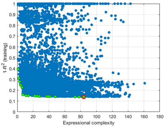
Figure 12.
Pareto front of models in terms of model performance and model complexity for a model with 3 genes and depth of up to 6.
In total, more potential architectures of the MGGP model were analyzed, that is, models with one, then two, three, four and five genes. For each model, the depth varies from one to a maximum of six. Using the evolutionary process, it creates a total of one million models for each type of model, and only the best 10,000 were displayed on the Pareto front. The number of model types is 30 (since we have models of up to five genes whose depth is from one to six, that gives 5 × 6 = 30 model types).
Figure 13 shows 19 Pareto optimal models out of a total of a million analyzed models that have a given structure of three genes (three trees) and whose tree depth is a maximum of six.
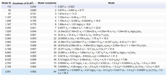
Figure 13.
Original output from the GPTIPS 2.0 software with analytical expressions of the models that make up the Pareto front (models with 3 genes and a maximum depth of generated trees of up to 6).
The results of all of the analyzed models in terms of the defined criteria are graphically presented in the Figure 14. It can be seen that in terms of RMSE and R criteria, the optimal model is composed of three genes whose tree depth is limited to six. Regarding the MAE criteria, the optimal model is composed of four genes whose depth is limited to four. While in terms of the MAPE criteria, it was found that the model with three genes and whose tree depth was limited to six was the most accurate. Regarding expression complexity, the optimal model is a model with four genes and a depth of up to three, whose expression complexity is the lowest and amounts to 39. The value of expression complexity is given automatically by the GPTIPS 2.0 software. Details regarding the model with four genes and whose tree depth is a maximum three are given in Appendix A (Figure A1, Figure A2 and Figure A3), while for the model with four genes whose tree depth is four, details are given in Appendix B (Figure A4, Figure A5 and Figure A6).
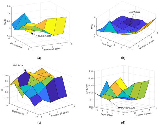
Figure 14.
Comparison of accuracy criteria for the MGGP model as a function of gene number and tree depth (a) RMSE, (b) MAE, (c) R, and (d) MAPE.
The specific analysis did not single out one model as the most accurate in terms of all defined criteria of accuracy, so a multicriteria analysis (Table 5) was used to rank the potential solutions. In order to select a multicriteria optimal solution, the approach was to try to select a solution that, to the greatest extent, satisfies all the criteria of accuracy, and does not have extremely bad criteria indicators, according to individual criteria.
Table 5.
Values of criterion functions for individual models or alternatives.
In addition, priority was given to finding a solution that has a lower complexity of expressions. The complexity of the expression is defined by the expressional complexity value given by GPTIPS 2.0 [27,28] software. As a methodological approach, the VIKOR method for finding compromise solutions was implemented. In this way, the search for a multicriteria compromise optimal solution was started.
When applying the VIKOR method, it was assumed that all criteria have the same weight, which is = 0.2, (i = 1, 2, …, 5). Since the criteria space is heterogeneous, i.e., criteria expressed in different units, all values are first scaled into the interval [0, 1]. The length of the range of the i-th criterion function is , where for each i-th criterion, corresponds to the best alternative system (or decision) and the worst. For creating dimensionless functions (Table 6) with an interval range from criteria functions [0, 1], the following transformation is used here (20):
Table 6.
Normalized and weighted normalized values of criterion functions.
Using the normalized values, the following metric values can be obtained:
The VIKOR method introduces a modified measure by adding to the value obtained in the previous expression a value of the quantity , which is determined on the basis of the following relation:
From here, the values of the modified measure R are obtained:
Based on the defined metrics S and R, the problem is reduced to a two-dimensional one, and by adopting the same preference for satisfying the majority of criteria as for each individual criterion (), a compromise ranking list of solutions can be obtained (Table 7).
Table 7.
Ranking of individual alternatives using the metrics of the VIKOR method.
By analyzing Table 7. it can be seen that the final order of alternatives based on metric Q has the following order . In order for alternative to be considered as the only compromise solution to the problem, it is necessary that the difference in Q measures for alternatives and be greater than the threshold value DQ = 0.25, which is satisfied in this case, so it can be considered that represents the only compromise solution to the optimization problem. In addition, satisfies both conditions and . The accuracy of the proposed compromise solution, according to the adopted criteria, is given in Table 8 and its structure is as in Figure 15.
Table 8.
Comparative analysis of results of different machine-learning models.
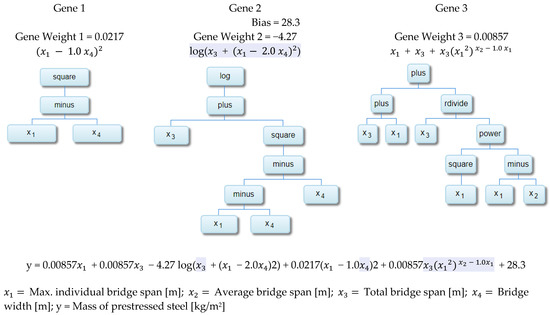
Figure 15.
Tree structure of the individual genes that comprise the optimal model (gene = 3, depth = 6).
Diagrams of modeled and actual values on the training set are shown in the Figure 16a), while the values of the modeled and actual values on the test dataset are shown in the Figure 16b).
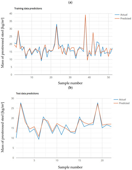
Figure 16.
Graphic representation of modeled (optimal model gene = 3, depth = 6) and actual values of prestressed steel consumption: (a) training set, (b) testing set.
5. Conclusions
The paper defines models based on regression trees that can be used to forecast the amount of prestressed steel in the construction of prestressed concrete bridges. Defined models do not require the use of certain software or the possession of programming knowledge and can be very easily applied in practice. In addition, the analyzed models showed higher accuracy compared to neural network models recommended by many studies.
The application of defined symbolic models in the form of constitutive equations is quick. The structure of the model and its parameters are extracted directly from the data in this study, as opposed to the standard regression models, which first specify the model’s structure before determining its parameters from the experimental data. The resulting model, which takes the form of scaled trees and represents a linear combination of nonlinear input transformations, can effectively simulate the challenging task of estimating the consumption of prestressed steel during the construction of prestressed concrete bridges.
The accuracy of the model expressed through the value of the MAPE error of 9.16%, as well as the high value of the correlation coefficient of 94.29%, was obtained.
The formed mathematical model recognized the span as a variable that implicitly contains information about the type of bridge construction (for example, precast beams or box girder). The representation of different types of construction was unbalanced, so this information could not be entered as an input. However, since the authors are working on increasing the database, it will be implemented in the future research.
In this research, MGGP models proved to be significantly simpler and more accurate than ANN models. There is a significantly larger number of ANN model parameters that need to be determined, significant analysis is required when determining the optimal structure, and their implementation requires some programming knowledge. The RT models that were analyzed have less complexity than the ANN model, however, the form of the model itself, being in the form of a complex tree, is not ideal for practical application. MGGP models have an advantage over both ANN and RT models in that their structure is determined by the data itself without any subjective action.
The model developed in the paper can be applied within the range of the dataset on which it was developed.
The limitations of the paper are that the bridges within the database were realized in a relatively narrow geographical area. In that area, there are no significant differences in bridge load (seismic load, wind load, etc.). If there are significant differences in model loading during model training, an additional input variable could be introduced to the training dataset that would include this.
Although the database of prestressed bridges, in this case, is composed of data on 74 completed bridges, it can be considered significant. Expanding the database would result in more data within the training and test dataset, which could define the model and its accuracy even more precisely.
The research applied in this paper has, in terms of results compared to previous research, produced a result that is generally better than the other researched models in terms of criteria of accuracy and complexity. Furthermore, the obtained model is straightforward and is in the form of a simple equation.
In the event of a significant increase in the database in future research, clustering methods could also be applied. The methodology developed in this work would be applied in individual clusters, and individual equations can be defined for each cluster type. The mentioned methodology can also be applied to the similar problem of determining constitutive equations in engineering and construction when we have enough experimental data for the problem we are considering.
Author Contributions
Conceptualization, M.K. and F.A.; methodology, M.K. and F.A.; software, M.K.; validation, M.K. and F.A.; formal analysis, M.K.; investigation, M.K.; resources, M.K. and F.A.; data curation, M.K.; writing—original draft preparation, M.K.; writing—review and editing, M.K. and F.A.; visualization, M.K. and F.A.; supervision, M.K. and F.A.; All authors have read and agreed to the published version of the manuscript.
Funding
This research received no external funding.
Data Availability Statement
The data presented in this study are available on request from the corresponding author.
Conflicts of Interest
The authors declare no conflict of interest.
Appendix A

Figure A1.
Pareto front of models in terms of model performance and model complexity for a model with 4 genes and depth up to 3.

Figure A2.
Original output from the GPTIPS 2.0 software with analytical expressions of the models that make up the Pareto front (models with 4 genes and a maximum depth of generated trees of up to 3).

Figure A3.
Graphic representation of modeled (model gene = 4, depth = 3) and actual values of prestressed steel consumption: (a) training set and (b) testing set.
Appendix B

Figure A4.
Pareto front of models in terms of model performance and model complexity for a model with 4 genes and depth up to 4.

Figure A5.
Original output from the GPTIPS 2.0 software with analytical expressions of the models that make up the Pareto front (models with 4 genes and a maximum depth of generated trees of up to 4).

Figure A6.
Graphic representation of modeled (model gene = 4, depth = 4) and actual values of prestressed steel consumption: (a) training set and (b) testing set.
References
- Pržulj, M. Mostovi; Udruženje Izgradnja: Beograd, Srbija, 2014; pp. 1–7. [Google Scholar]
- Tayefeh Hashemi, S.T.; Ebadati, O.M.; Kaur, H. Cost Estimation and Prediction in Construction Projects: A Systematic Review on Machine Learning Techniques. SN Appl. Sci. 2020, 2, 1703. [Google Scholar] [CrossRef]
- Tang, Y.; Wang, Y.; Wu, D.; Liu, Z.; Zhang, H.; Zhu, M.; Chen, Z.; Sun, J.; Wang, X. An experimental investigation and machine learning-based prediction for seismic performance of steel tubular column filled with recycled aggregate concrete. Rev. Adv. Mater. Sci. 2022, 61, 849–872. [Google Scholar] [CrossRef]
- Feng, W.; Wang, Y.; Sun, Y.; Tang, Y.; Wu, D.; Jiang, Z.; Wang, J.; Wang, X. Prediction of thermo-mechanical properties of rubber-modified recycled aggregate concrete. Constr. Build. Mater. 2022, 318, 125970. [Google Scholar] [CrossRef]
- Zhao, X.Y.; Chen, J.X.; Chen, G.M.; Xu, J.J.; Zhang, L.W. Prediction of ultimate condition of FRP-confined recycled aggregate concrete using a hybrid boosting model enriched with tabular generative adversarial networks. Thin. Wall. Struct. 2023, 182 Pt B, 110318. [Google Scholar] [CrossRef]
- Antoniou, F.; Aretoulis, G.; Giannoulakis, D.; Konstantinidis, D. Cost and Material Quantities Prediction Models for the Construction of Underground Metro Stations. Buildings 2023, 13, 382. [Google Scholar] [CrossRef]
- Flyvbjerg, B.; Skamris, H.; Buhl, S. Underestimating Costs in Public Works Projects: Error or Lie? J. Am. Plan. Assoc. 2002, 68, 279–295. [Google Scholar] [CrossRef]
- Menn, C. Prestressed Concrete Bridges; Birkhauser Verlag: Basel, Switzerland, 1990. [Google Scholar]
- Marcous, G.; Bakhoum, M.M.; Taha, M.A.; El-Said, M. Preliminary Quantity Estimate of Highway Bridges Using Neural Networks. In Proceedings of the Sixth International Conference on the Application of Artificial Inteligence to Civil and Structural engineering, Stirling, Scotland, 19–21 September 2001. [Google Scholar]
- Liolios, A.; Kotoulas, D.; Antoniou, F.; Konstantinidis, D. Egnatia Motorway bridge management systems for design, construction and maintenance. In Advances in Bridge Maintenance, Safety and Management—Bridge Maintenance, Safety, Management, Life-Cycle Performance and Cost; CRC Press: Boca Raton, FL, USA, 2006; pp. 135–137. [Google Scholar] [CrossRef]
- Fragkakis, N.; Lambropoulos, S.; Tsiambaos, G. Parametric Model for Conceptual Cost Estimation of Concrete Bridge Foundations. J. Infrastruct. Syst. 2011, 17, 66–74. [Google Scholar] [CrossRef]
- Antoniou, F.; Konstantinitis, D.; Aretoulis, G. Cost Analysis and Material Consumption of Highway Bridge Underpasses. In Proceedings of the Eighth International Conference on Construction in the 21st Century (CITC-8), Changing the Field: Recent Developments for the Future of Engineering and Construction, Thessaloniki, Greece, 27–30 May 2015. [Google Scholar]
- Antoniou, F.; Konstantinidis, D.; Aretoulis, G.; Xenidis, Y. Preliminary construction cost estimates for motorway underpass bridges. Int. J. Constr. Manag. 2017, 18, 321–330. [Google Scholar] [CrossRef]
- Antoniou, F.; Konsantinidis, D.; Aretoulis, G. Analytical formulation for early cost estimation and material consumption of road overpass bridges. Int. J. Res. Appl. Sci. Eng. Technol. 2016, 12, 716–725. [Google Scholar] [CrossRef]
- Antoniou, F.; Marinelli, M. Proposal for the Promotion of Standardization of Precast Beams in Highway Concrete Bridges. Front. Built Environ. 2020, 6, 119. [Google Scholar] [CrossRef]
- Marinelli, M.; Dimitriou, L.; Fragkakis, N.; Lambropoulos, S. Non-Parametric Bill of Quantities Estimation of Concrete Road Bridges Superstructure: An Artificial Neural Networks Approach. In Proceedings of the 31st Annual ARCOM Conference, Lincoln, UK, 7–9 September 2015. [Google Scholar]
- Kovačević, M.; Ivanišević, N.; Petronijević, P.; Despotović, V. Construction cost estimation of reinforced and prestressed concrete bridges using machine learning. Građevinar 2021, 73, 1–13. [Google Scholar] [CrossRef]
- Kovačević, M.; Bulajić, B. Material Consumption Estimation in the Construction of Concrete Road Bridges Using Machine Learning. In Proceedings of the 30th International Conference on Organization and Technology of Maintenance (OTO 2021), Osijek, Croatia, 10–11 December 2021; Lecture Notes in Networks and Systems. Springer: Cham, Switzerland, 2021; Volume 369. [Google Scholar] [CrossRef]
- Kovačević, M.; Ivanišević, N.; Stević, D.; Marković, L.M.; Bulajić, B.; Marković, L.; Gvozdović, N. Decision-Support System for Estimating Resource Consumption in Bridge Construction Based on Machine Learning. Axioms 2023, 12, 19. [Google Scholar] [CrossRef]
- Kovačević, M.; Lozančić, S.; Nyarko, E.K.; Hadzima-Nyarko, M. Application of Artificial Intelligence Methods for Predicting the Compressive Strength of Self-Compacting Concrete with Class F Fly Ash. Materials 2022, 15, 4191. [Google Scholar] [CrossRef] [PubMed]
- Ripley, B.D. Statistical Aspects of Neural Network, Networks and Chaos-Statistical and Probabilistic Aspects; Barndoff-Neilsen, O.E., Jensen, J.L., Kendall, W.S., Eds.; Chapman & Hall: London, UK, 1993. [Google Scholar]
- Kaastra, I.; Boyd, M. Designing a neural network for forecasting. Neurocomputing 1996, 10, 215–236. [Google Scholar] [CrossRef]
- Kanellopoulas, I.; Wilkinson, G.G. Strategies and best practice for neural network image classification. Int. J. Remote Sens. 1997, 18, 711–725. [Google Scholar] [CrossRef]
- Heaton, J. Introduction to Neural Networks for C#, 2nd ed.; Heaton Research, Inc.: Chesterfield, MO, USA, 2008. [Google Scholar]
- Sheela, K.G.; Deepa, S.N. Review on methods to fix number of hidden neurons in neural networks. Math. Probl. Eng. 2013, 2013, 425740. [Google Scholar] [CrossRef]
- Hastie, T.; Tibsirani, R.; Friedman, J. The Elements of Statistical Learning; Springer: Berlin/Heidelberg, Germany, 2009. [Google Scholar]
- Breiman, L.; Friedman, H.; Olsen, R.; Stone, C.J. Classification and Regression Trees; Chapman and Hall/CRC: Wadsworth, OH, USA, 1984. [Google Scholar]
- Poli, R.; Langdon, W.; Mcphee, N. A Field Guide to Genetic Programming; Lulu Enterprises, UK Ltd.: London, UK, 2008. Available online: http://www0.cs.ucl.ac.uk/staff/W.Langdon/ftp/papers/poli08_fieldguide.pdf (accessed on 15 December 2022).
- Searson, D.P.; Leahy, D.E.; Willis, M.J. GPTIPS: An Open Source Genetic Programming Toolbox for Multigene Symbolic Regression. In Proceedings of the International MultiConference of Engineers and Computer Scieintist Vol. I, IMECS 2010, Hong Kong, China, 17–19 March 2010. [Google Scholar]
- Searson, D.P. GPTIPS 2: An open-source software platform for symbolic data mining. In Handbook of Genetic Programming Applications; Springer: Berlin/Heidelberg, Germany, 2015; pp. 551–573. [Google Scholar]
- Searson, D.P.; Willis, M.J.; Montague, G.A. Co-evolution of non-linear PLS model components. J. Chemom. 2007, 2, 592–603. [Google Scholar] [CrossRef]
- Searson, D.P.; Willis, M.J.; Montague, G.A. Improving controller performance using genetically evolved structures with co-adaptation. In Proceedings of the Eighteenth IASTED International Conference on Modelling, Identification and Control, Innsbruck, Austria, 15–18 February 1999; ACTA Press: Anaheim, CA, USA, 1999. Available online: https://citeseerx.ist.psu.edu/viewdoc/download?doi=10.1.1.152.9591&rep=rep1&type=pdf (accessed on 8 January 2023).
- Antoniou, F. Delay Risk Assessment Models for Road Projects. Systems 2021, 9, 70. [Google Scholar] [CrossRef]
- Aretoulis, G.; Papathanasiou, J.; Antoniou, F. PROMETHEE based ranking of project managers’ based on the five personality traits. Kybernetes 2020, 49, 1083–1102. [Google Scholar] [CrossRef]
- Opricović, S. Optimizacija Sistema; Građevinski Fakultet: Beograd, Srbija, 1992. [Google Scholar]
- Opricović, S. Višekriterijumska Optimizacija Sistema u Građevinarstvu; Građevinski Fakultet: Beograd, Srbija, 1998. [Google Scholar]
- Opricović, S.; Tzeng, G.H. Extended VIKOR method in comparison with outranking methods. Eur. J. Oper. Res. 2007, 178, 514–529. [Google Scholar] [CrossRef]
- Zeleny, M. Compromise Programming, Multiple Criteria Decision Making; University of South Carolina Press: Columbia, SC, USA, 1973. [Google Scholar]
- Kovačević, M. Application of Compromise Programming in Evaluation of Localities for Construction of Municipal Landfill. In Interdisciplinary Advances in Sustainable Development, 1st ed.; ICSD 2022; Lecture Notes in Networks and Systems; Tufek-Memišević, T., Arslanagić-Kalajdžić, M., Ademović, N., Eds.; Springer: Cham, Switzerland, 2022; Volume 539. [Google Scholar] [CrossRef]
Disclaimer/Publisher’s Note: The statements, opinions and data contained in all publications are solely those of the individual author(s) and contributor(s) and not of MDPI and/or the editor(s). MDPI and/or the editor(s) disclaim responsibility for any injury to people or property resulting from any ideas, methods, instructions or products referred to in the content. |
© 2023 by the authors. Licensee MDPI, Basel, Switzerland. This article is an open access article distributed under the terms and conditions of the Creative Commons Attribution (CC BY) license (https://creativecommons.org/licenses/by/4.0/).