Article

An Efficient Construction Method of the 3D Random Asphalt Concrete Model Based on the Background Grid and the Moving-and-Densifying Algorithm

School of Civil Engineering, Central South University, Changsha 410075, China
*
Author to whom correspondence should be addressed.
Buildings 2023, 13(4), 990; https://doi.org/10.3390/buildings13040990
Submission received: 9 March 2023 / Revised: 4 April 2023 / Accepted: 6 April 2023 / Published: 8 April 2023
(This article belongs to the Special Issue Advanced Materials and Novel Technique in Civil Engineering)

Abstract

:
In order to avoid the tedious and time-consuming measuring process for thermal conductivity, many random models have been proposed, but the construction of those random models is still inefficient, which limits the further application. In this paper, a construction method of three-dimensional random asphalt models for predicting thermal conductivity based on the background grid and the moving-and-densifying algorithm was proposed which greatly improves construction efficiency. The influence of the random factors on models’ stability was studied and the range of the key factors within all random factors was restricted. Further, a conflict judgment method for the convex aggregate and the improved take-and-place method based on the background grid method and the moving-and-densifying algorithm was realized by MATLAB code to construct aggregate mixture models. Finally, the aggregate mixtures model was imported into ABAQUS 2022 to predict the thermal conductivity based on the steady-state plate method, and the validity of the predicting result was verified by experimental result. With this construction method, the stability index is improved by more than 80.71%, and packing efficiency is 198.98% higher than before. Additionally, the 3D random model showed a smaller prediction error range (less than 5%) than the 2D models (more than 10%) and was more accurate than the 2D prediction model. This research focused on improving the construction efficiency of the 3D random asphalt concrete model which contributes to full utilization and laying a foundation for further improvement.

1. Introduction

As a prominent construction material, asphalt concrete is widely used in all aspects of civil engineering. Along with the rapid development of the discrete element method (DEM) and the finite element method (FEM), many researchers have developed a series of numerical models to predict some properties of asphalt concretes [1,2,3,4,5,6]. Thermal conductivity is among the most important properties of asphalt concrete, and a lot of mesoscale numerical models have been developed to aid prediction [4,5,7,8]. Most prediction models are two-dimensional (2D) models and differ greatly from reality. Some other researchers have constructed three-dimensional (3D) thermal conductivity prediction models, but the construction efficiency of those models is relatively low. Therefore, it is very important to improve the construction method of the prediction model to meet the requirement of efficiency and accuracy in real cases. The key to efficiently constructing a 3D model is to improve the construction efficiency of the aggregate mixture model which includes the generation and packing of aggregates in sequence.
Two main methods are currently used for the construction of the aggregates model. One is based on image recognition, applying computer tomography (CT) equipment to scan the real aggregate to obtain a more accurate geometric model [9,10,11]. Although an accurate and realistic aggregate model can be obtained by this method, it is not only expensive but also time consuming. In particular for the 3D aggregate model, a large number of 3D aggregate databases need to be constructed, which greatly reduces the usefulness of the image scanning method. Another method is to construct a random geometric model of aggregates based on the geometric characteristics of aggregates and the Monte Carlo algorithm. This method was widely used for the ability to generate aggregate models quickly and massively [2,5,12]. The difficulty in constructing a random geometric model lies in the description of aggregates’ geometric characteristics. For the two-dimensional aggregate model, researchers usually replace the aggregates with simple geometric shapes such as circles [6,13,14], ellipses, and polygons. Additionally, for a 3D aggregate model, various geometric features of aggregates were selected as the random factors to construct an aggregate model randomly and in reality. However, too many random factors could lead to massive computational difficulty in model construction [6,15,16]. Most researchers utilized three to four random factors to control the shape of the aggregate model and constructed the aggregate model either directly or in two steps [17,18], thus the aggregate models had enough randomness while the amount of computation was greatly reduced. However, the simplified random model showed numerous undesirable geometric features such as being needle like and sharpness [19], which led to unsatisfactory stability and additional computational difficulty.
The keys to packing aggregates are the judgment function of the conflicted relationship in aggregates and the packing algorithm. The packing algorithm varies according to the geometric characteristics of the aggregate. For a two-dimensional aggregate model, due to less computation, the commonly used packing method is the take-and-place method, and its conflict judgment method often applies the analytical method, the Gilbert–Johnson–Keerthi distance algorithm, and other methods [6,19]. The take-and-place method is a “fill-in” algorithm, which means the random aggregate is placed one by one through the Monte Carlo method. If placed successfully, the coordinates of the aggregates are recorded; otherwise, coordinates are re-selected until the aggregates are placed. Because of its nature of filling vacancies, its packing efficiency will decrease with the decrease in vacancies, and this method is more applicable in the less calculation two-dimensional model. The packing methods are more diverse for the 3D aggregate model. Zhao et al. [20] imported aggregate models into PFC3D to achieve a denser packing of aggregates within a set time by setting boundary conditions and applying loads. However, the low computational efficiency limits its usefulness. In addition, some researchers took the take-and-place method as the packing algorithm [21,22]. However, the problem where the packing efficiency of the take-and-place method decreases with an increase in the placed aggregates still exists. Many studies have improved the packing efficiency of the take-and-place method. Ouyang et al. [23] imported the background grid to reduce the unnecessary placement of the take-and-place method. Zhou et.al and Zhang et al. [24,25] made the model denser by applying displacement to the placed aggregates. Although those studies have improved a certain defect of the take-and-place method, few studies simultaneously improved both the defects.
In this study, a more stable aggregate geometry-generating method and a more efficient packing method were proposed to construct the 3D random model with less computation and meet the requirement of the practice. Firstly, several random factors were set, and the range of those random factors was reasonably restricted with the index of stability. Secondly, the aggregate model was constructed with high randomness and enough stability based on the restricted random factors. Thirdly, a conflict judgment method for convex polyhedral aggregates and an improved take-and-place method combining the background grid method and the moving-and-densifying (MAD) algorithm were proposed and realized by MATLAB code. Finally, the generated geometric model was constructed by the above methods and imported into the ABAQUS 2022 to construct the thermal conductivity prediction model, and the accuracy of the prediction model was verified by the experiment results.

2. Generation of 3D Random Model

2.1. The Aggregates Target Volume for Model Generation

The target volume of different size grade aggregates is the upper limit for the aggregate generation which could be determined by gradation and specimen size. The grading curve used in this study is shown in Figure 1, where Gradation 1#, Gradation 2#, and Gradation 3# denote three different gradations of the asphalt concrete. The specimen size was set to 100 mm × 100 mm × 75 mm, the bitumen content of asphalt concrete is 4%, and the bitumen content of asphalt mortar is 8.32%. The gradation curve is the mass percentage curve, which can be converted to the target volume of different size grade Vi, according to Equation (1).
V i = ( p i p i + 1 ) ( 1 V a i r ) V s p e c i m e n ( 1 + m a ) V a l l ρ i V a l l = i = 1 n p i p i + 1 ( 1 + m a ) ρ i
where Vi is the target volume of the ith size grade of aggregates; pi, pi+1 is the passing ratio of the ith size grade; Vair is the porosity of the specimen, which is defined as 0.04 in this paper; Vspecimen is the total volume of the specimen; ma is the mass fraction of asphalt. In this study, ma for asphalt mortar and asphalt concrete is defined as 4% and 8.32%; ρi is the density of the ith size grade aggregate, which is defined as 2600 kg/m3; Vall is the percentage of aggregate volume to the sum of asphalt volume and aggregate volume.

2.2. Aggregate Generation

In this study, the aggregate was defined as a convex polyhedron with 16 to 20 vertices partly because 3D convex polyhedrons are more consistent with the geometric characteristics of general mineral aggregates than spheres and ellipsoids, and partly to simplify the modeling process of aggregates and reduce the amount of computation.
Some random factors (such as the shape coefficient η, spherical radius r, number of vertices n, and the vertex random distribution factor ζ) are set as the control condition for the aggregate generation to improve the randomness for aggregate models. Based on the relationship between each factor and the stability of the aggregate model the random distribution factor ζ was distributed in [0.4, 0.9] and the shape coefficient η was distributed in [1.46, 1.73]. The construction steps of the random convex aggregate model are as follows. Firstly, the vertices of an aggregate were selected from a random size sphere surface, and the vertices number of the upper hemisphere can be determined by Equation (2).
n 1 i = r o u n d 0.5 × n i + ζ × w
where the ni is the total number of vertices of the ith aggregate, and its value is an integer between 16 and 20; the round function serves to round the expressions in parentheses; the ζ is a random factor with a value that is distributed in [0.4, 0.9]; w is a fluctuation factor, and the larger its value, the greater the difference in the distribution of vertices on the upper and lower hemispheres, and w is defined as 2 in this paper; n1i is the number of vertices in the upper hemisphere of the ith aggregate. Accordingly, the number of vertices in the lower hemisphere of the ith aggregate, n2i is defined as
n 2 i = n i n 1 i
Secondly, in the spherical coordinates system, the azimuth of each vertex before stratification can be calculated by Equations (4) and (5) according to n1i and n2i.
1 i j = 2 π / n 1 i + r a n d ( 1 ) × π × ζ / n 1 i
2 i j = 2 π / n 2 i + r a n d ( 1 ) × π × ζ / n 2 i
where rand(1) function serves to create a random value between 0 and 1; Φ1ij and Φ2ij represent the azimuth values of the jth vertex of the upper and lower hemispheres of the ith aggregate before stratification, respectively. Additionally, then the vertices of the upper and lower hemispheres are stratified by Equations (6) and (7), respectively.
φ 1 i j = k = 1 j φ 1 i k + 1 i j × o × π / j = 1 n 1 i 1 i j
φ 2 i j = k = 1 j φ 2 i k + 2 i j × o × π / j = 1 n 1 i 2 i j
where φ1ij and φ2ij are the azimuth values of the jth vertex of the upper and lower hemispheres of the ith aggregate, respectively; o is the total azimuthal angle after stratification, and o is defined as 4π in this paper. Further, the value of the zenith angle of each vertex is obtained by Equations (8) and (9).
θ 1 i j = π 4 + u × φ 1 i j 2 π | φ 1 i j 2 π | × r a n d ( 1 )
θ 2 i j = π 4 + u × φ 2 i j 2 π | φ 2 i j 2 π | × r a n d ( 1 )
where θ1ij and θ2ij are the azimuths of the jth vertex of the ith aggregate on the upper and lower hemispheres, respectively. Then, the vertex coordinates of the aggregates are converted from the spherical coordinates to the Cartesian coordinates by Equation (10).
x i j y i j z i j = r i × sin θ 1 i j × c o s ( φ 1 i j ) r i × sin θ 1 i j × s i n ( φ 1 i j ) r i × cos θ 1 i j 0 < j < n 1 i x i j y i j z i j = r i × cos θ 2 i j × c o s ( φ 2 i j ) r i × cos θ 2 i j × s i n ( φ 2 i j ) r i s i n θ 2 i j n 1 i < j < n 2 i
where xij, yij, zij are the Cartesian coordinate values of the jth vertex of the ith spherical aggregate; ri is the random radius of the ith spherical aggregate and can be obtained by Equation (11).
r i = 0.25 × r a n d 1 × d m i n + 0.25 × r a n d 1 × ( d m a x d m i n )
where dmin and dmax are the lower and upper limits of the size grade, respectively. Finally, the shape coefficient η is used to further control the aggregate shape with the Equation (12).
X i j = x i j × ( η ( 1 ) + r a n d ( 1 ) × ( 1 η ( 1 ) ) ) Y i j = y i j × ( η ( 2 ) + r a n d ( 1 ) × ( 1 η ( 2 ) ) ) Z i j = z i j × ( η ( 3 ) + r a n d ( 1 ) × ( 1 η ( 3 ) ) )
where η(1), η(2), and η(3) are the three components of the η, the mold of the shape coefficient is distributed in [1.458, 1.732] and the value of η(1) is 1, which means 2.13 < (1 + η(2)2 + η(3)2) < 3; Xij, Yij, Zij are the Cartesian coordinate values of the jth vertex of the ith random convex aggregate. Furthermore, the discrete vertex coordinates of aggregates were transformed into triangles pair by the Delaunay triangulation function and convex hull algorithm and output in the stl format [26].
The flowchart of aggregate generation is shown in Figure 2, where num is the number of aggregates; VVa is the total volume of aggregates in this cycle; VVb is the total volume of aggregates in the previous cycle; n is the number of aggregate size grade. When generating an aggregate, the vertices coordinate information is determined by the above process, the volume V is obtained by the Delaunay triangulation function within MATLAB. Additionally, in each loop, the total volume VVa and the volume limitation was compared to make sure that the generated aggregate model is consistent with the designed gradation curve shown in Figure 1. Additionally, the volume limitations for each size grade of aggregates can be obtained from Section 2.1.

2.3. Packing of Aggregates

There are two defects that led to the low packing efficiency of the take-and-place method. First, the random placement makes the aggregate loosely distributed in the placement space and forms many small voids among the aggregates, which leads to increased difficulty in packing aggregates. Second, the success rate of the placement selection decreases as the proportion of placed aggregates increases. The improved take-and-place method improves the two defects through the background method and the moving-and-densifying algorithm.
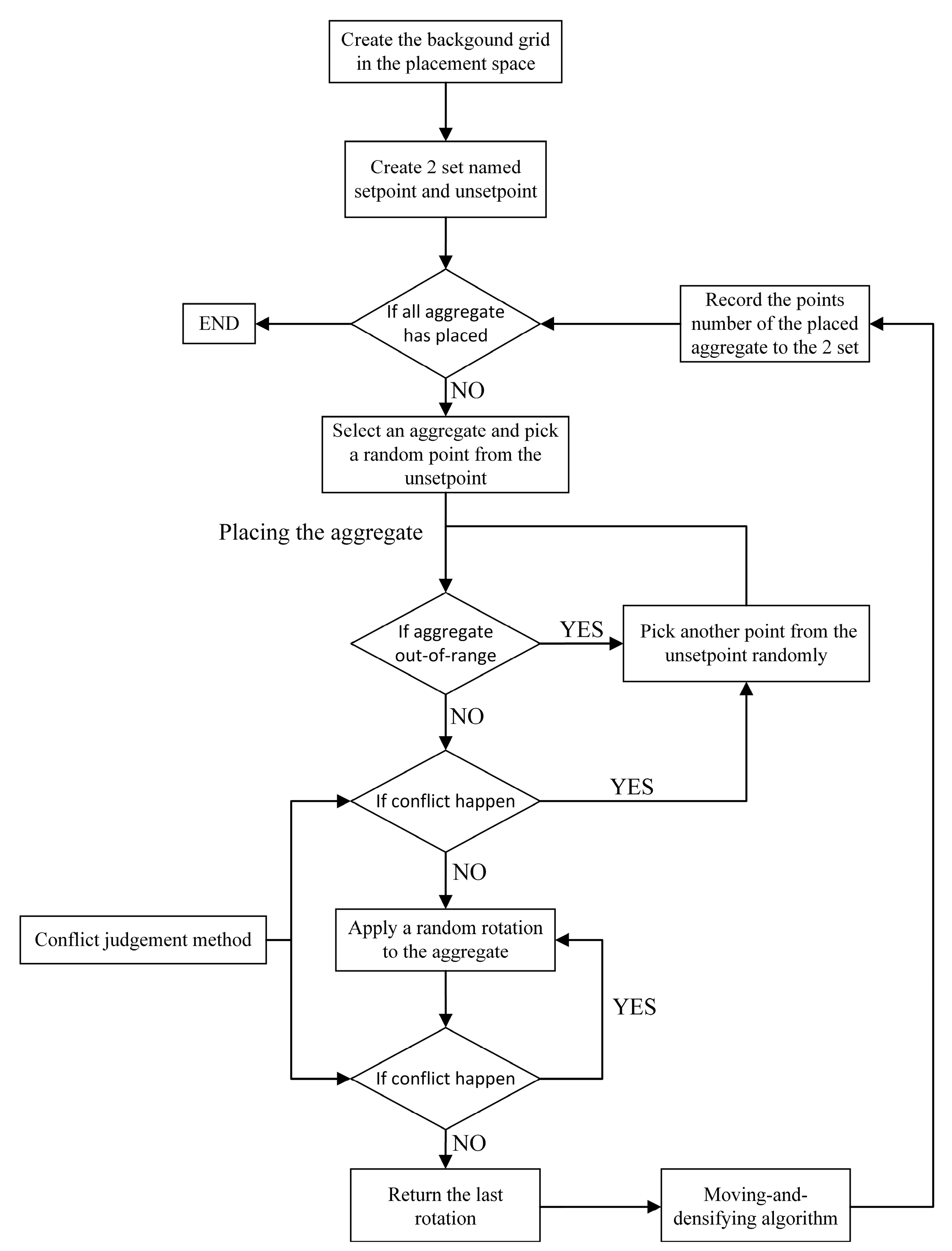
Figure 3 shows the flowchart of the packing process, and the steps of the improved take-and-place method are as follows. Firstly, the background grid was created in the placement space, which means the placement space was discretized into many points, and each point owns a unique serial number. Secondly, two sets named setpoint and unsetpoint are created to record the serial numbers of placed aggregates and unplaced aggregates, and the transition from any point coordinate to the serial number can be realized by Equation (20). Thirdly, select an aggregate generated in Section 2.2 and pick a random point from the unsetpoint, then place the chosen aggregate to the chosen point which can be realized by coordinate calculation (superposition of aggregate and random point coordinates). After that, the location of the aggregate was judged, to make sure all coordinate of the aggregate was in the range of the placement space. Then, acquire the points information of the aggregate through the conflict judgment method introduced in this section and retrieve the repeat serial number of the aggregate from the setpoint. If there is no repeat serial number in the newly placed aggregate, random rotations are applied to the placed aggregate to densify the placement space until the conflict happens. The random rotations could be generated by Equation (13) and applied to the aggregates by Equation (14).
M = cos α 0 sin α 0 1 0 sin α 0 cos α 1 0 0 0 cos β sin β 0 sin β cos β c o s γ s i n γ 0 s i n γ c o s γ 0 0 0 1
p t s = p t s · M
where M is the rotation matrix; α, β, and γ are the rotation angles in the x, y, and z directions, respectively, which are taken as a random angle between 0° and 45° in this study; pts is the vertex coordinates of the aggregates.
Then, return the last rotation to keep the aggregate from conflict and utilize the MAD algorithm to further densify the placement space, where the process of the MAD algorithm can be seen in Figure 4. The point numbers of the placed aggregates are recorded to the setpoint and removed from the unsetpoint. After that, determine whether all aggregates in Section 2.2 have been placed; if so, output all aggregate coordinate data in the stl format; otherwise, start from the third step.
The MAD algorithm was used to make the newly placed aggregate closer to the placed aggregates with several rotations and displacements. Additionally, the steps are as follows. First, apply random displacement [I, J, K] to the newly placed aggregate until the conflicts happen, where I, J, and K are integers between −1 and 1. Second, apply a rotation M to the aggregate and then create k to record the number of rotations applied on the aggregate. After each rotation is applied, make a judgment about the conflicts; and if not, record the coordinate information of the aggregate and stop the MAD algorithm. Otherwise, repeat the second step until the k reaches the maximum trying times (in this study, it was set as 10), then record the coordinate information of the aggregate and stop the MAD algorithm.
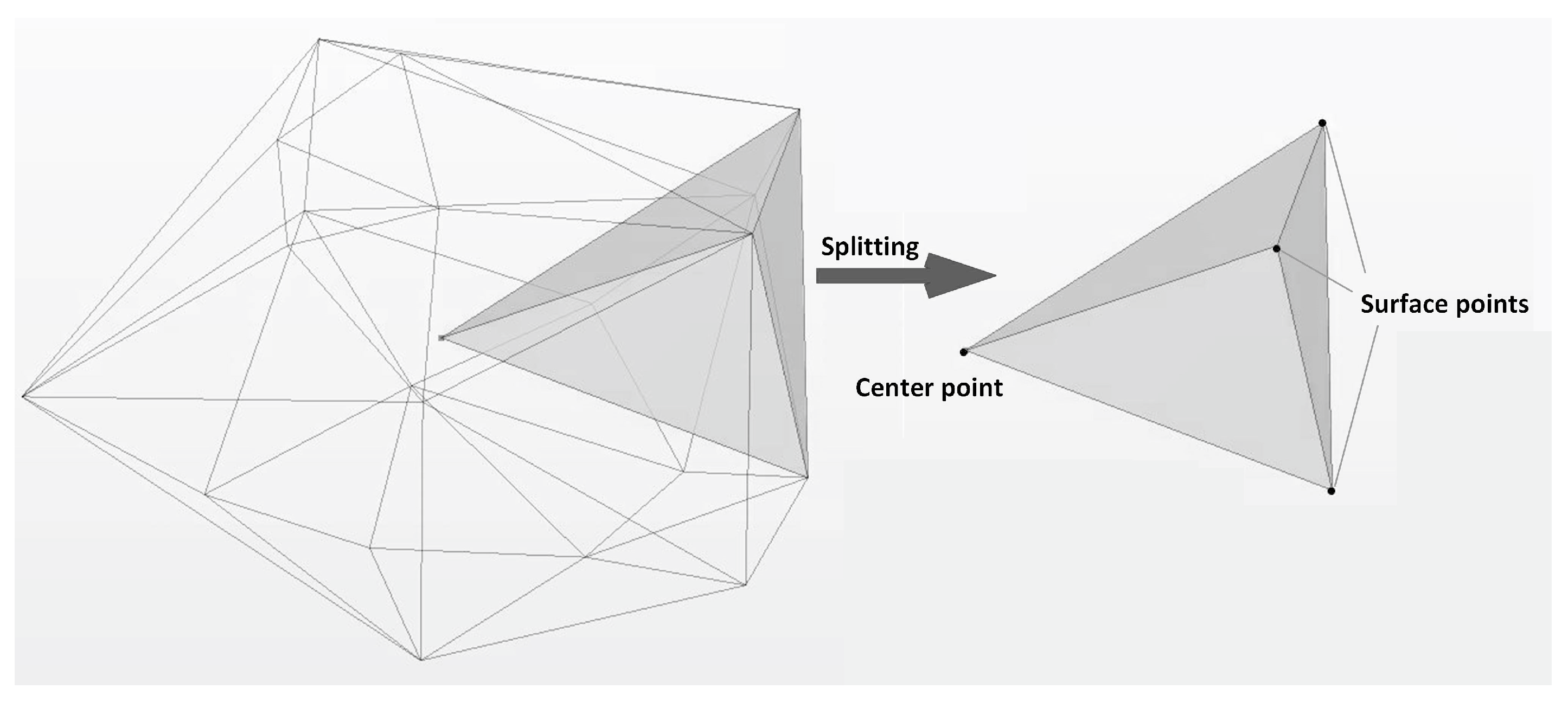
In order to improve the accuracy, an aggregate conflict judgment method was proposed based on the geometric properties of 3D convex aggregates. The complex geometric problems were transformed into simple algebraic problems by splitting the aggregate model. Firstly, the convex polyhedral aggregate was split into dozens of tetrahedrons containing the surface triangles and the center point, which can be realized by the Delaunay triangulation function. Figure 5 is the schematic of aggregate splitting. Secondly, the vertex coordinates of the tetrahedron were substituted into Equation (15) to obtain the vertex equation for each tetrahedron.
f 1 2 f 2 + f 1 + f 3 3 v + f 1 2 f 2 + f 1 3 v = 0
where the f1, f2, and f3 are intermediate variables that can be calculated by Equation (16), Equation (17) and Equation (18), respectively, and the tetrahedral volume v can be calculated by Equation (19).
f 1 = x y z 1 x 1 y 1 z 1 1 x 2 y 2 z 2 1 x 3 + x 4 2 y 3 + y 4 2 z 3 + z 4 2 1
f 2 = x y z 1 x 1 y 1 z 1 1 x 2 + x 3 2 y 2 + y 3 2 z 2 + z 3 2 1 x 2 + x 4 2 y 2 + y 4 2 z 2 + z 4 2 1
f 3 = x y z 1 x 2 y 2 z 2 1 x 3 y 3 z 3 1 x 4 y 4 z 4 1
v = x y z 1 x 1 x 2 x 3 x 4 y 1 y 2 y 3 y 4 z 1 z 2 z 3 z 4
where x1, y1, z1, x2, y2, z2, x3, y3 and z3 are the coordinates of the three vertices of the surface triangle of the convex polyhedron; x4, y4, z4 are the coordinates of the center point of the convex polyhedron. The analytic equation set for convex aggregates could be formed by combining all the vertex equations which can be used to judge if the point coordinated by (x,y,z) located in the aggregate. Substituting the coordinates of the arbitrary point coordinates into the analytic equation set for calculating, if there was a non-negative value in the result, the point is surrounded by the aggregate. The BGM discretized the placement space into many points. Thus, the coordinates of aggregates’ points can be determined by substituting all the points that located in the calculation area into the analytic equation set. Furthermore, the coordinates of aggregates’ points were converted into serial numbers with Equation (20). Additionally, the conflicted relationship among aggregates could be judged by determining whether the serial numbers of the newly placed aggregate and that of the placed area were repeated.
num = xc/coordi(1) + yc/coordi(2) × NumX + zc/coordi(3) × NumX × NumY + 1
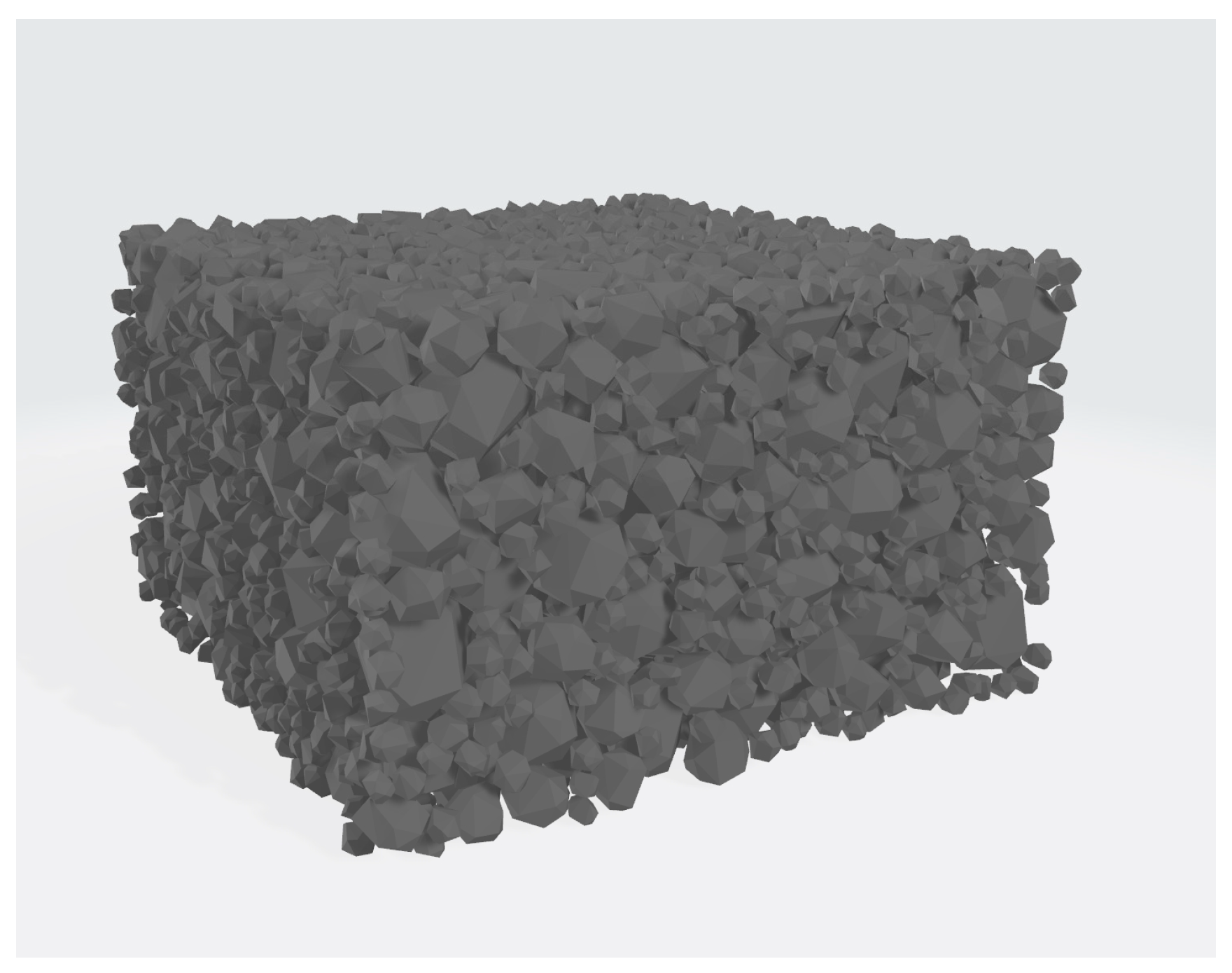
where num is the serial number of points, coordi(1), coordi(2), and coordi(3) are the spacing of discrete points in the x, y, and z directions, respectively, and NumX and NumY are the point numbers in the x and y direction; xc, yc, zc are the coordinates. In order to reduce the amount of computation in the simulation, the generated aggregate mixture model only contains the first three sizes of the gradation. Figure 6 is the constructed aggregate mixture model.
In this chapter, both defects of the take-and-place method were improved based on the background grid method and the moving-and-densifying algorithm which improved the generation efficiency of a random model and meet the requirement of real cases. Additionally, a novel analytic conflict judgment method focused on convex polyhedral was proposed, which provide a new approach to judge the conflict of geometry model.

3. Construction of the Thermal Conductivity Predicting Model

3.1. Method Selection

The transient method and the steady-state method were developed to measure thermal conductivity, both of which are based on Fourier’s heat transfer equation The transient method has the advantages of simple operation and shorter test time, which is more suitable for practical application, while the steady-state method has a simple model and is more adaptable to simulation. Many studies [15,27] have found that the difference between the transient and steady-state methods for asphalt concretes was less than 5% and it mainly came from the accuracy of the experimental instruments and the errors formed by improper environmental control. Additionally, different test methods show little difference for the unmodified asphalt concrete [28]. Therefore, the steady-state plate method was used in the simulation of thermal conductivity, and the transient plane source method (TPS) was used for the verification test of thermal conductivity.

3.2. Determination of Thermal Conductivity

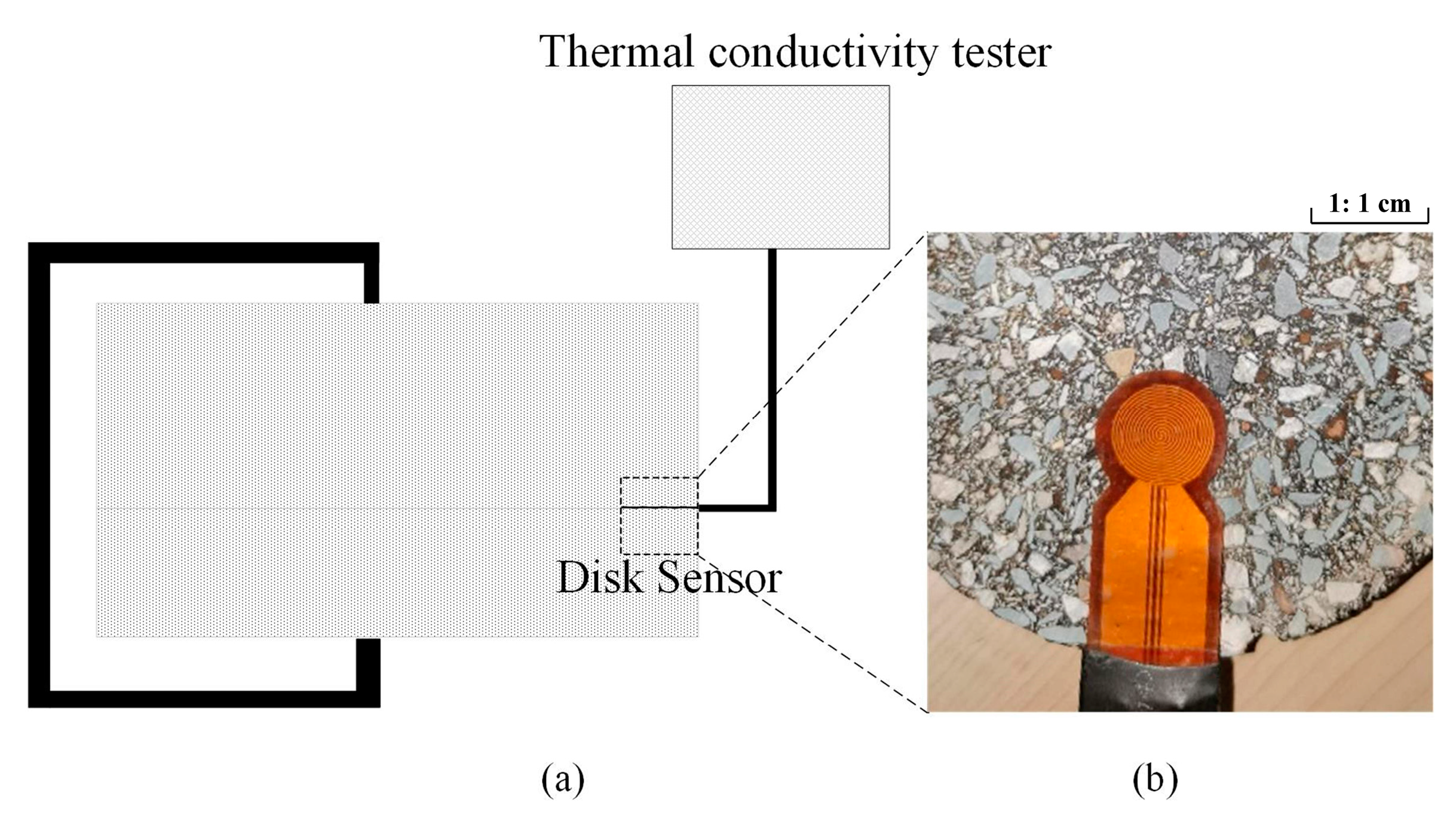
The geometric model of the asphalt concrete is set as a two-phase structure, including the continuous phase consisting of asphalt mortar and pores, as well as the dispersed phase of the first three grade aggregates. The thermal conductivity of asphalt concrete and asphalt mortar was obtained as the parameters required for simulation and model validation with the TPS method. The schematic of the TPS method is shown in Figure 7. The test temperature was 20 °C, and the test device was DRE 2C produced by XIANGTAN INSTRUMENT company. In this study, the limestone was used as coarse aggregate, and its thermal properties were derived from the literature [29,30,31], and the specific heat capacity of asphalt mortar and asphalt concrete was calculated by Equation (21)
C v = C v b i t u m e n × P b i t u m e n + C v a g g r e g a t e × P a g g r e g a t e
where Cv is the calculated specific heat capacity, Paggregate and Pbitumen denote the mass fraction of aggregates and bitumen, and Cvaggregate and Cvbitumen denote the specific heat capacity of aggregates and bitumen, which are set to 850 (J/(kg·K) and 1000 (J/(kg·K) in this study according to Zou et al. [32]. The gradations of asphalt mortar and asphalt concrete used in the thermal conductivity test are shown in Figure 1. The gradation of asphalt mortar was set as 2.08 times the gradation of asphalt concrete below 4.75 mm to ensure that the thermal conductivity of the asphalt mortar was consistent with that of the continuous phase of the asphalt concrete.
Three Φ 63.5 mm × 101 mm cylindrical specimens were prepared for asphalt mortar and 3 gradations of asphalt concrete separately, and two cross-sections were cut in every specimen. To ensure the accuracy of thermal conductivity measurement, three different measuring points were randomly selected from the same cross-sections. Table 1 lists the thermal properties obtained through experiments as well as from the literature.

3.3. Construction of the Element Model

In the finite element software, the finest aggregate with full details takes more than 90% units due to the big quantity and small mesh when meshed with the model of the first four size grade aggregate. In order to add more grades of aggregate, the aggregate models were transformed into element models, which means the aggregate model will be replaced by several elements in the same location. The process was shown in Figure 8. Firstly, the placement space was dispersed into numbered elements. Creating a set to record the element number of aggregate, the element belonging to aggregate models can be calculated by Equation (15). Then, the element of the mortar was generated with the Boolean operations, which means removing the elements belonging to aggregate from all the numbered elements.
The steady-state plate method is a method for determining the thermal conductivity by constructing the one-dimensional steady heat conduction. The schematic diagram of the test device is shown in Figure 9a. The specimen is surrounded by a hot plate, a cold plate, and the insulation layer. During the experiment, the hot plate is applied to a constant heat flow while the cold plate is kept constant temperature, which creates a one-dimensional steady heat conduction process from the hot plate to the cold plate. Figure 9b shows the finite element model for the steady-state plate method, by using the model shown in Figure 9b, the thermal conductivity of the asphalt concrete is predicted as follows:
Firstly, the properties (include thermal conductivity, specific thermal capacity, and density) of aggregates and asphalt mortar were given. Secondly, the DC3D20 (the 20-node linear hexahedral thermal conductivity element) was applied to the element model for the thermal transfer calculation. Thirdly, since the one-dimensional steady-state heat transfer process of the model, creating a steady-state analysis step and setting the interrelationships to thermal contact. Additionally, then, a heat flow of 1 W/m2 was applied on the heating plate and a temperature boundary condition of 15 °C was applied on the cooling plate of the model. Finally, the job was submitted to obtain the temperature field of the model, and the thermal conductivity of the specimen is calculated by Equation (22).
λ = q h Δ T
where the λ is the thermal conductivity of the specimen, W/(m·K), q is the heat flow rate of the heating plate input, W/m2; h is the height of the specimen, m; ∆T is the temperature difference between the upper and lower surfaces of the specimen, °C.

4. Prediction Results and Validation

In this study, three different gradations of asphalt concrete were simulated, and the gradations of aggregates are shown in Figure 1. Three different specimens for each gradation were prepared with the process introduced in Section 3.3. The thermal conductivity of limestone aggregates and asphalt mortar was set to the mean value shown in Table 1, which is 2.58 W/(m·K) and 1.90 W/(m·K), respectively.
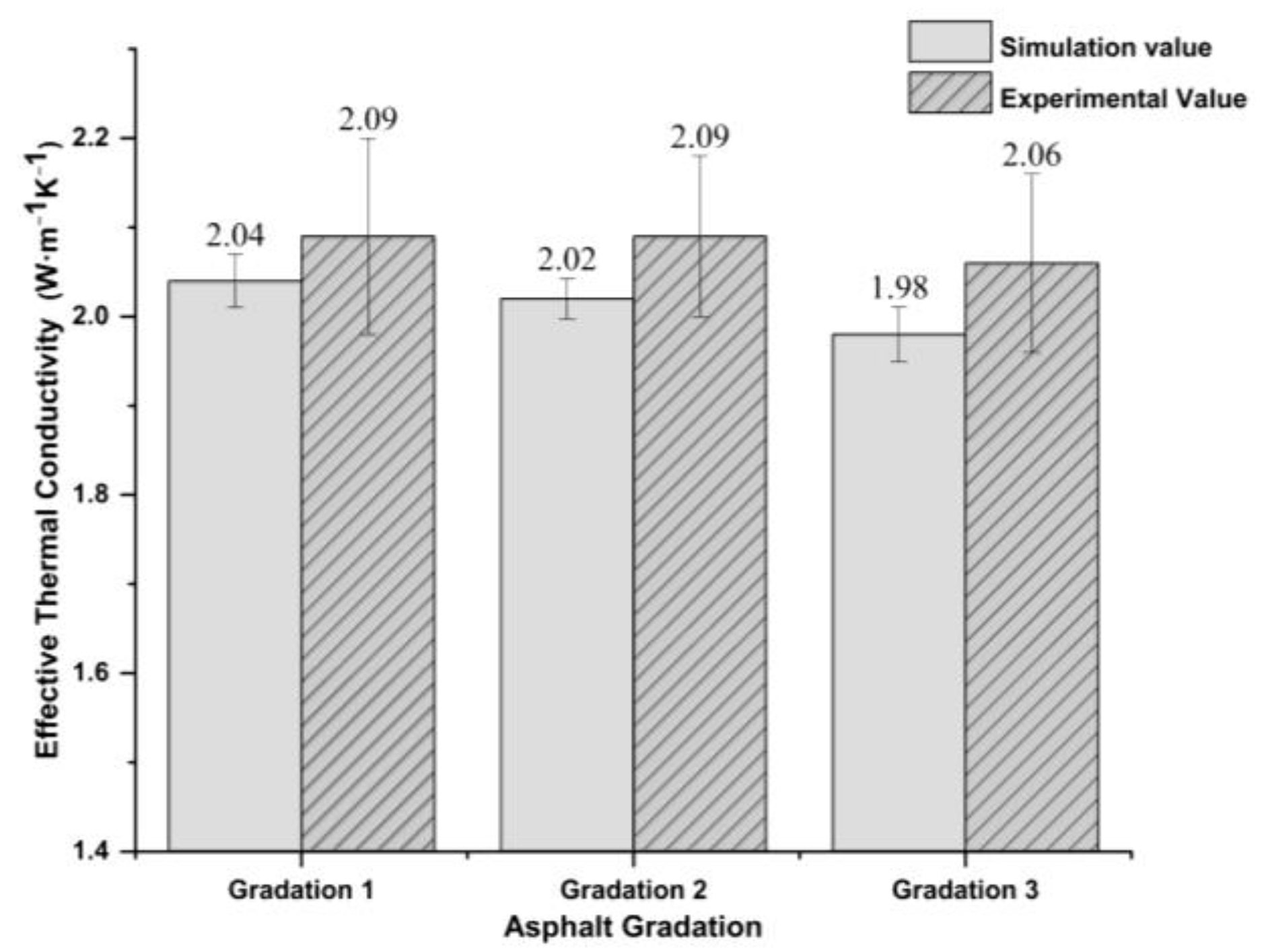
The average temperature on the hot surface and cold surface can be calculated with the plug-in volume-weighted average temperature. Then, the average temperatures of both the upper and lower surfaces of each specimen were substituted into Equation (23) to calculate the thermal conductivity. Figure 10 shows the prediction results for thermal conductivity.
R E i = 100 × | 1 λ i λ e x p |
where REi denotes the relative error between the simulated value and the experimental value, %; λi is the average value of simulated thermal conductivity, and λexp is the average value of experimental thermal conductivity, W/(m·K). The RE value of all the simulation value can be calculated from Figure 10, the maximum RE value is 3.88%, the average RE value for all gradations is 3.21%, and the value range of RE is less than 5%. Additionally, from Figure 10, we know that in simulation, the gradation and the distribution of aggregates have no significant effect on the thermal conductivity. Additionally, in the experiment, the thermal conductivity changes a lot with the test value. Because the thermal conductivity is very changeable in asphalt concrete. Additionally, the TPS method can just acquire the thermal conductivity of the test point, thus repeated and random measurements are required. Therefore, the prediction model could be a more accurate and efficient method to acquire the thermal conductivity of a mixture such as asphalt concrete. Table 2 shows the 2D thermal conductivity prediction models constructed by other studies. The maximum RE value was 16.58%, the minimum RE value was 1.44%, and the value range of RE is more than 10% which was because the 2D prediction model acquires the thermal conductivity from a random section, and a section was hard to represent the whole specimen. Thus, the 3D random model in this study was more closed to the real value of thermal conductivity than the 2D model and showed less prediction error than the TPS method. That is, we could acquire a more accurate prediction value of the thermal conductivity through the 3D random model.

5. Discussions

5.1. Restricted of Geometry Random Factors Based on the Stability

In order to ensure that the generated aggregate model has both high randomness and sufficient stability, on one hand, multiple random factors were set to improve the aggregate model with the randomness, where the random factor included the shape coefficient η, spherical radius r, number of vertices n, and the vertex random distribution factor ζ. On the other hand, the range of some key random factors was restricted to improve the aggregate models’ stability reasonably. Additionally, the initial range of each random factor is shown in Table 3. Since the shape coefficient is a 3D vector, only the range of its mold (|η|) is restricted in Table 3 while the direction angle is not restricted.
Aggregate models with higher stability have less undesirable geometric features (such as sharpness and needle- like). When packing aggregates with the same gradation of Gradation 2# shown in Figure 1, the aggregate model with the factor range listed in Table 4 generated 5813 pieces and the packing time was 5522 s. Additionally, the aggregate model with the factor range listed in Table 3 generated 6041 pieces and the packing time was 5780 s. Thus, the stability has a significant impact on packing efficiency because the poor stability model generates more pieces of aggregates and requires more packing time, and reducing the stability of the aggregate model is a feasible way to improve packing efficiency.
The stability of the aggregate model can be improved by restricting the value range of random factors. However, different random factors have a different influence on the stability. In order to obtain the key factors and make a reasonable restriction, the effect of each random factor on the stability of the aggregate models was studied. The number of small edges and small facets of the geometric model is used as the index to evaluate the model’s stability. It is expressed by defect, which is defined as follows.
d e f e c t = d e f e c t l < 0.1 d m i n + d e f e c t ( s < 0.01 d m i n 2 )
where the defect denotes the total number of aggregate defects, dmin is the lower limit of aggregate size grade, defect(l < 0.1 dmin) is the total number of edges with a length that is less than 0.1 dmin, and defect(s < 0.01 d m i n 2 ) is the total number of facets with an area less than 0.01 d m i n 2 .
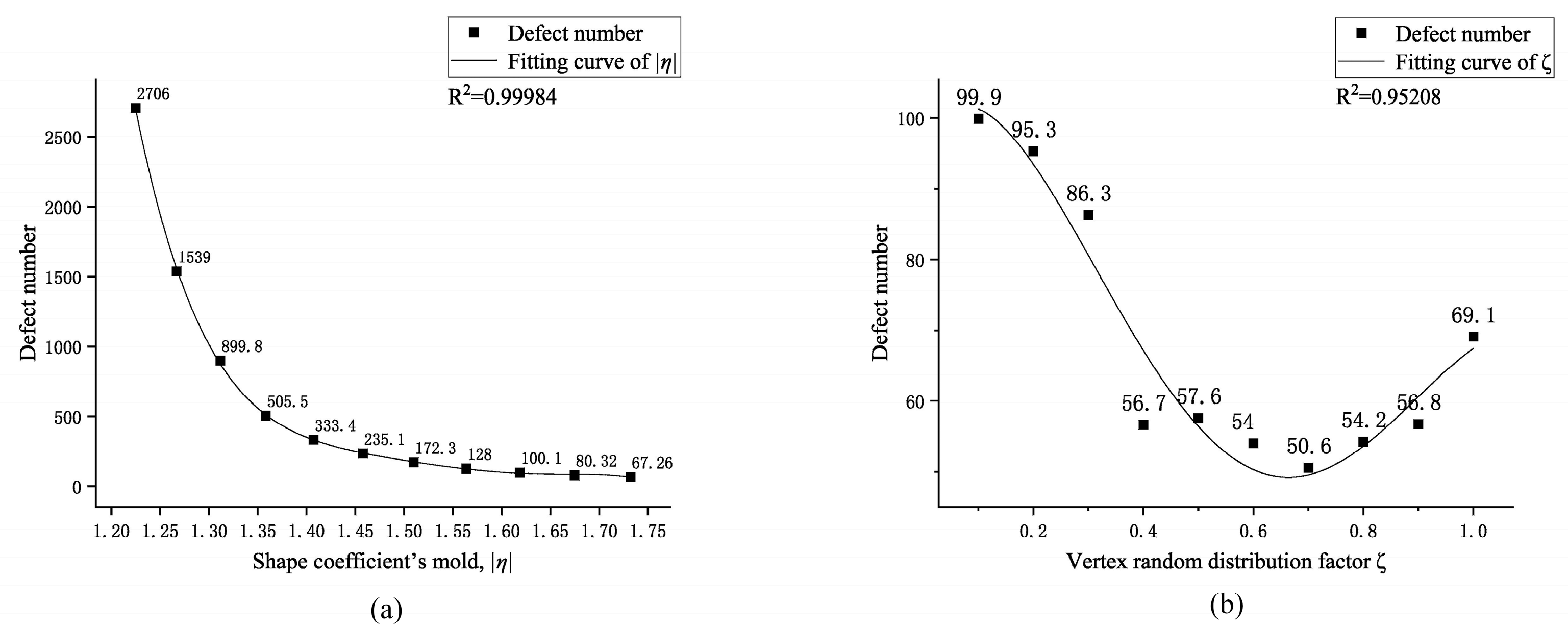
The control variable method was used to study the relationship between each random factor and model stability. In every simulation, only the random factor to be studied is changed and other factors remain unchanged, and the aggregate models with a volume of 50,000 mm3 were generated and the defect number of the models was counted. The simulation was repeated 100 times for each data point, and the mean value was taken as the representative value. According to the fitting relationship between random factors and the defect, the random factors were divided into linear and non-linear related random variables. Linearly related random variables are shown in Figure 11a,b and non-linearly related random variables are shown in Figure 12a,b.
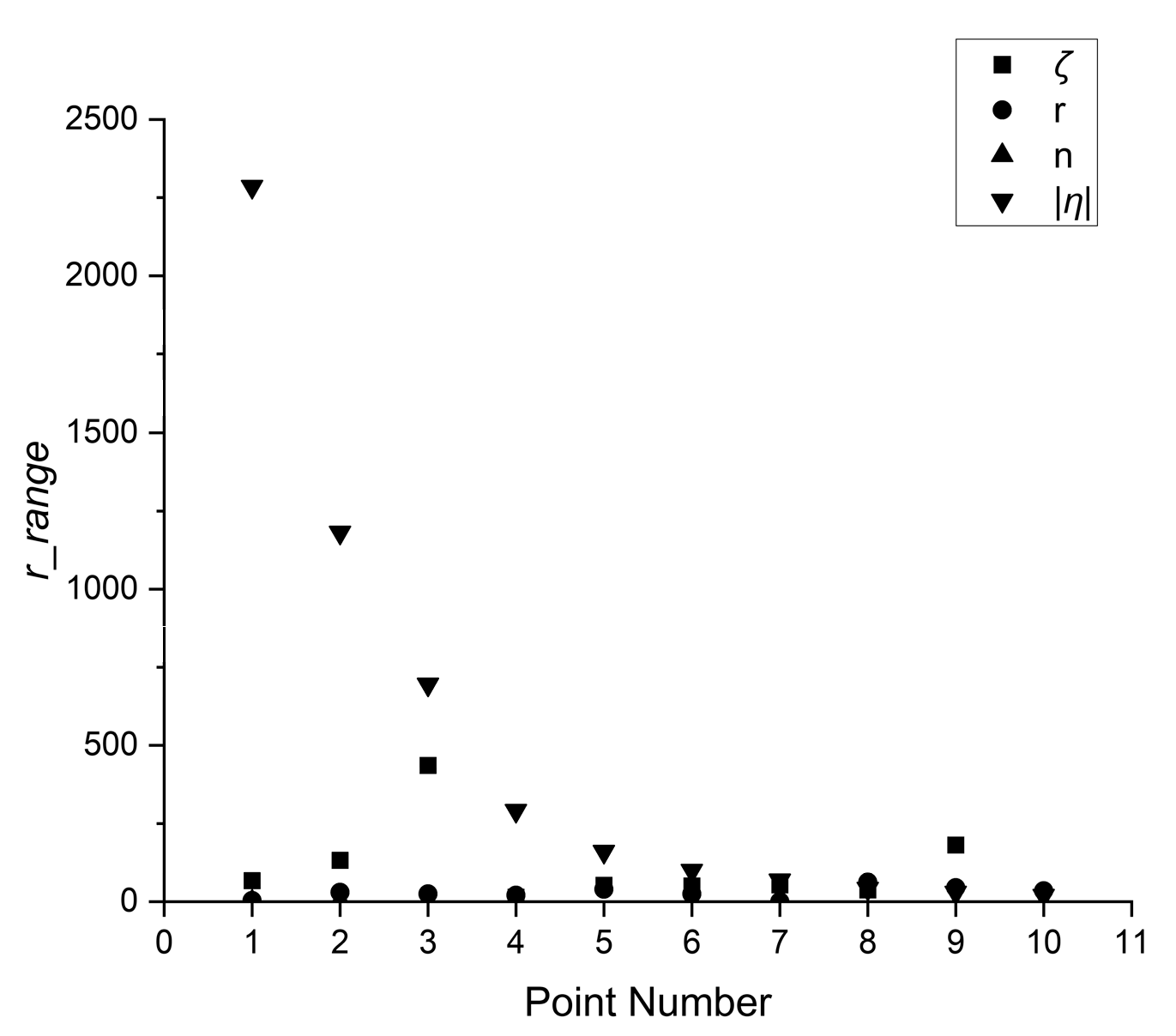
The percentage of the restricted range to the total range is expressed by P, which is used to quantitatively describe the randomness. Additionally, the relative range is expressed by r_range, which is used to quantitatively describe the stability of random factors. The r_range is defined as follows.
r _ r a n g e = d e f e c t m e a n v a l u e × p e r c e n t a g e × 100 %
where r_range is the relative range of the data point, percentage is the percentage of each data point’s range to the entire range, and the meanvalue is the mean value of each random factor’s defect. The r_range of the spherical radius r and the number of vertices n are 28.07% and 2.67%, respectively; and the r_range of the |η| and the ζ are 428.99% and 72.45%, respectively. Additionally, the r_range of every random factor in each data point is shown in Figure 13.
It can be seen that the effect of both the linearly related random variables on stability are not as significant as the two non-linearly related random factors. Additionally, for the linearly related random variables, through restricting the value range, the increase in stability is also linearly related to the loss of randomness. Therefore, the ζ and the |η| are taken as the key random factors, and only the range of those key random factors is restricted. Additionally, Table 4 shows the property comparison of ζ and |η| properties before and after the restriction. After the restriction on the value range, the r_range value of the |η| and ζ is reduced by 70.52% and 99.50%, respectively; and the mean value of the |η| and ζ is reduced by 80.71% and 18.70%, respectively.

5.2. Efficiency Improvement of the Packing Algorithm

5.2.1. Efficiency Improvement of the Improved Take-and-Place Method

The essence of the BGM is to discretize the placement space into a finite number of points, which enables the recording and the calling of the placed aggregates during the packing process. According to the BGM, this study divided the placement space into the placed area and the unplaced area. Additionally, the placement points were selected only in the unplaced area, which avoids the defect of repeated selection in the placed area and thus greatly improved the success rate of the placement selection.
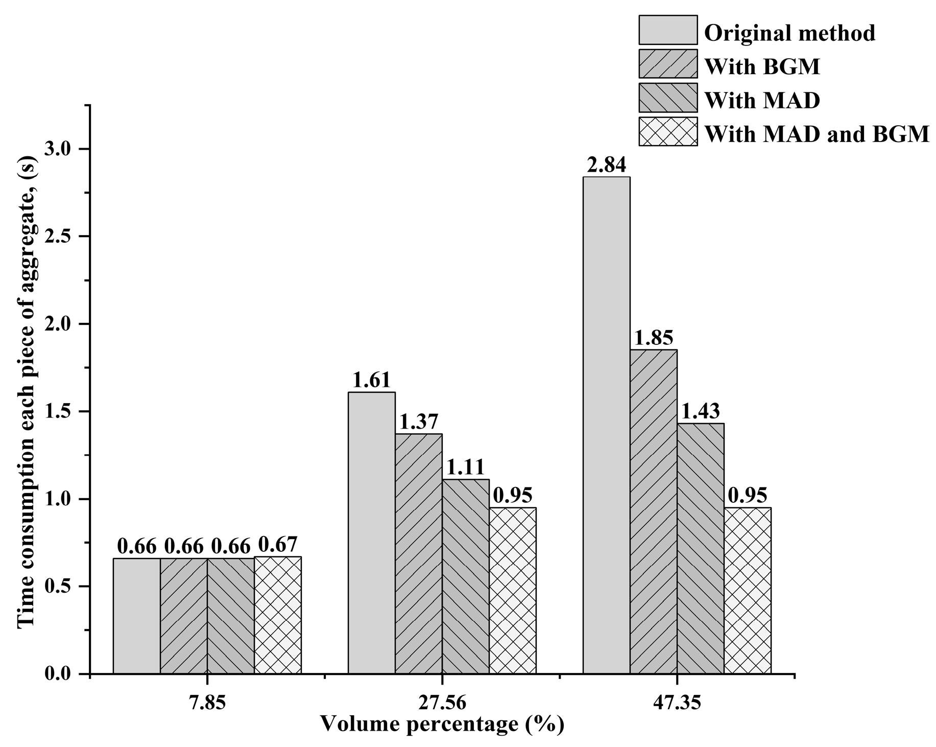
The size of the placement space is set as 100 mm × 100 mm × 75 mm; as a result, the volume of the first five grades of aggregates is 78,468 mm3, 197,118 mm3, 197,921 mm3, 143,192 mm3, and 62,011 mm3, respectively. Additionally, the aggregate number of the first five particle size grades is 53, 259, 806, 4695, and 22,107, respectively. Figure 14 shows the time consumption of each work condition for placing each piece of aggregate with the increasing volume percentage. In Figure 14, the original method follows the process shown in Figure 3, but does not create the background grid nor adopt the MAD algorithm to the placed aggregate. Accordingly, the method with the BGM does not adopt the MAD algorithm to the placed aggregate, the method with MAD does not create the background grid, and the method with the MAD and BGM algorithms follows the process shown in Figure 3.
For the BGM, with the increase in the volume percentage of the placed area, the influence of the property that only selects placement point in the unplaced area on the placement efficiency increases, and the placement efficiency is increased by 53.5% when the volume percentage of the placed area reaches 47.35%, which means the packing method with the BGM can place 1.535 pieces of aggregates while the original method can just place 1 piece of aggregate at the same time.
In this study, additional displacement and rotation were applied to the placed aggregate by the MAD algorithm to compensate for the defects of the loose aggregate distribution of the take-and-place method, which increased the capacity of the placement space and improved the placement efficiency. As the results in Figure 14, when the volume percentage of placed area is 7.85%, the efficiency difference between the take-and-place method with the MAD algorithm and the original one is only 2.20%. When the volume percentage of the placed area reaches 47.35%, the efficiency difference expands to 98.70%, which means the MAD algorithm greatly improves the placement efficiency of the model.
The packing efficiency of the improved take-and-placed method with the BGM and the MAD algorithms was 198.98% higher than that of the original one when the placed area reached 47.35%. Additionally, packing efficiency increased with the increase in placed area.

5.2.2. Efficiency Improvement by Minimizing the Calculation Area

The conflict judgment function was called repeatedly in the packing process, so its computational efficiency was very important for packing efficiency. The operation time of the conflict judgment function is closely related to the point number contained in the calculation area, and the amount of computation for conflict judgment can be greatly reduced by minimizing the calculation area.
Due to the randomness of aggregate shape, if the maximum aggregate size is used as the basis for dividing the calculation area, the additional amount of computation is generated. In this study, the size of each aggregate was taken as the basis for dividing the conflict judgment area to improve calculational efficiency. The maximum coordinate differences of the aggregate in the x, y, and z directions are rounded upwards and set as the length, width, and height of the cuboid calculation area, respectively. Additionally, the setting area precisely surrounds the convex polyhedral aggregate. By minimizing the calculation area, the average time used for single conflict judgment of the first three grades of aggregates is reduced to 0.3646 s from 0.4635 s. Additionally, the calculational efficiency of the conflict judgment function for the first three grades of aggregates was improved by 27.13%.

6. Conclusions

In this paper, a method that could efficiently construct a 3D random asphalt concrete model for predicting the thermal conductivity of asphalt concrete was proposed to improve construction efficiency. The main conclusions are summarized as follows:
  • A four-random-factors aggregate generation method was proposed, and the key factors in the four random factors were confirmed with the index of defect number. In this case, the key factors include the mold of the shape coefficient |η| and the vertex random distribution factor ζ. By restricting the value range of the key factors, the relative variation ranges of the stability index were reduced by 70.52% and 99.50%, respectively, and the averages were reduced by 80.71% and 18.70%, respectively.
  • The take-and-place method was improved by the BGM and the MAD algorithms, respectively, and the packing efficiency of both methods increased with the increase in the aggregate volume percentage. When the volume percentage of aggregates reached 47.35%, the packing efficiency of the take-and-place method with the MAD algorithm was 98.65% higher than that of the original take-and-place method, the take-and-place method with the BGM improved packing efficiency by 53.5%, and the packing efficiency of the improved method with the BGM and MAD algorithms was 198.98% higher than that of the original take-and-place method.
  • A conflict judgment method for convex polyhedral aggregates was proposed. Additionally, the increase in computational efficiency for conflict judgment reached 27.13% by minimizing the calculation area.
  • The thermal conductivity of the asphalt concrete model was simulated by the steady-state plate method. Compared with the experimental measurements, the maximum prediction error of the 3D random models was 3.88%, and the average was 3.21%. The 3D random model showed a smaller prediction error range (less than 5%) than the 2D models (more than 10%) and was more accurate than the 2D prediction model.
  • It is important to adjust the developed model for use in real cases; although packing efficiency was greatly improved by this construction method the two-phase structure ignored the impact of the pore in the asphalt concrete which should be studied in further work. Further, the aggregate generation method can be replaced with a more efficient or real method to meet the requirement of the application. Additionally, further studies should investigate the application of the random models in other properties of asphalt concrete.

Author Contributions

Conceptualization, X.L.; Methodology, X.L. and Y.Z.; Software, H.C.; Validation, H.C. and Y.Z.; Investigation, H.C.; Resources, Y.Z.; Writing—original draft, H.C.; Writing—review & editing, X.L. and Y.Z.; Supervision, X.L. All authors have read and agreed to the published version of the manuscript.

Funding

This work was supported by the National Natural Science Foundation of China (No. 52078499) and the Natural Science Foundation of Hunan province (No. 2022JJ30930), the Transportation Science and Technology Project of Hunan province (No. 202246).

Data Availability Statement

Some or all data, models, or code that support the findings of this study are available from the corresponding author upon reasonable request—1. the code of the packing algorithm using in this article; 2. the code of the moving-and-densifying algorithm.

Conflicts of Interest

The authors declare no conflict of interest.

References

  1. Wang, D.; Ding, X.; Gu, L.; Ma, T. Assessment Model and Virtual Simulation for Fatigue Damage Evolution of Asphalt Mortar and Mixture. Adv. Mater. Sci. Eng. 2018, 59, 4807. [Google Scholar] [CrossRef] [Green Version]
  2. Du, C.; Liu, P.; Sun, Y.; Chen, J.; Liu, Q.; Oeser, M. Characterizing asphalt mixtures with random aggregate gradations based on the three-dimensional locally homogeneous model. Comput.-Aided Civ. Infrastruct. Eng. 2022, 37, 1687–1702. [Google Scholar] [CrossRef]
  3. Szydlowski, C.; Gorski, J.; Stienss, M.; Smakosz, L. Numerical Simulation of Asphalt Mixtures Fracture Using Continuum Models. In Proceedings of the 22nd International Conference on Computer Methods in Mechanics (CMM), Lublin University of Technology, Lublin, Poland, 13–16 September 2017. [Google Scholar] [CrossRef]
  4. Chen, J.; Wang, H.; Dan, H.; Xie, Y. Random Modeling of Three-Dimensional Heterogeneous Microstructure of Asphalt Concrete for Mechanical Analysis. J. Eng. Mech. 2018, 144, 2505. [Google Scholar] [CrossRef]
  5. Han, D.; Liu, G.; Zhao, Y.; Pan, Y.; Yang, T. Research on thermal properties and heat transfer of asphalt mixture based on 3D random reconstruction technique. Constr. Build. Mater. 2021, 270, 121393. [Google Scholar] [CrossRef]
  6. Xu, J.; Zheng, C. Random generation of asphalt mixture mesostructure and thermal-mechanical coupling analysis at low temperature. Constr. Build. Mater. 2021, 280, 122537. [Google Scholar] [CrossRef]
  7. Mu, K.; Chen, J.; Mu, Q.; Garg, A.; Gao, Z.; Li, Y. Development of a microstructure-based numerical approach for analyzing heat transfer within the asphalt mixture. Constr. Build. Mater. 2020, 260, 119890. [Google Scholar] [CrossRef]
  8. Sun, Y.; Du, C.; Gong, H.; Li, Y.; Chen, J. Effect of temperature field on damage initiation in asphalt pavement: A microstructure-based multiscale finite element method. Mech. Mater. 2020, 144, 103367. [Google Scholar] [CrossRef]
  9. Yang, W. Finite element model of concrete material based on CT image processing technology. J. Vis. Commun. Image Represent. 2019, 64, 102631. [Google Scholar] [CrossRef]
  10. Sun, Y.; Zhang, Z.; Gong, H.; Zhou, C.; Chen, J.; Huang, B. 3D Multiscale Modeling of Asphalt Pavement Responses under Coupled Temperature-Stress Fields. J. Eng. Mech. 2022, 148, 2089. [Google Scholar] [CrossRef]
  11. Mora, C.F.; Kwan, A.K.H. Sphericity, shape factor, and convexity measurement of coarse aggregate for concrete using digital image processing. Cem. Concr. Res. 2000, 30, 351–358. [Google Scholar] [CrossRef]
  12. Ye, Y.; Sun, Y.; Gao, L.; Ma, Z.; Xue, X. Study On Creep Behavior Of Asphalt Mixture Based On Discrete Element Method. Balt. J. Road Bridge Eng. 2020, 15, 174–195. [Google Scholar] [CrossRef]
  13. Castillo, D.; Caro, S.; Darabi, M.; Masad, E. Influence of aggregate morphology on the mechanical performance of asphalt mixtures. Road Mater. Pavement Des. 2018, 19, 972–991. [Google Scholar] [CrossRef]
  14. Salemi, M.; Wang, H. Image-aided random aggregate packing for computational modeling of asphalt concrete microstructure. Constr. Build. Mater. 2018, 177, 467–476. [Google Scholar] [CrossRef]
  15. Yan, P.; Zhang, J.; Fang, Q.; Zhang, Y.; Fan, J. 3D numerical modelling of solid particles with randomness in shape considering convexity and concavity. Powder Technol. 2016, 301, 131–140. [Google Scholar] [CrossRef]
  16. Holla, V.; Vu, G.; Timothy, J.J.; Diewald, F.; Gehlen, C.; Meschke, G. Computational Generation of Virtual Concrete Mesostructures. Materials 2021, 14, 3782. [Google Scholar] [CrossRef]
  17. Du, C.; Sun, L.; Jiang, S.; Ying, Z. Numerical Simulation of Aggregate Shapes of Three-Dimensional Concrete and Its Applications. J. Aerosp. Eng. 2013, 26, 515–527. [Google Scholar] [CrossRef]
  18. Cao, P.; Jin, F.; Feng, D.; Zhou, C.; Hu, W. Prediction on dynamic modulus of asphalt concrete with random aggregate modeling methods and virtual physics engine. Constr. Build. Mater. 2016, 125, 987–997. [Google Scholar] [CrossRef]
  19. Huang, S.; Huang, L.; Lai, Z. An extension of the Fourier series-based particle model to the GJK-based contact detection and resolution framework for DEM. Comput. Part. Mech. 2022, 9, 381–391. [Google Scholar] [CrossRef]
  20. Zhao, L.; Zhang, S.; Huang, D.; Wang, X.; Zhang, Y. 3D shape quantification and random packing simulation of rock aggregates using photogrammetry-based reconstruction and discrete element method. Constr. Build. Mater. 2020, 262, 119986. [Google Scholar] [CrossRef]
  21. Yang, S.F.; Yang, X.H.; Yin, A.Y.; Jiang, W. Three-dimensional numerical evaluation of influence factors of mechanical properties of asphalt mixture. J. Mech. 2012, 28, 569–578. [Google Scholar] [CrossRef]
  22. Yin, A.; Yang, X.; Zeng, G.; Gao, H. Fracture simulation of pre-cracked heterogeneous asphalt mixture beam with movable three-point bending load. Constr. Build. Mater. 2014, 65, 232–242. [Google Scholar] [CrossRef]
  23. Ouyang, H.; Chen, X. 3D meso-scale modeling of concrete with a local background grid method. Constr. Build. Mater. 2020, 257, 119382. [Google Scholar] [CrossRef]
  24. Zhou, R.; Song, Z.; Lu, Y. 3D mesoscale finite element modelling of concrete. Comput. Struct. 2017, 192, 96–113. [Google Scholar] [CrossRef] [Green Version]
  25. Zhang, Z.; Song, X.; Liu, Y.; Wu, D.; Song, C. Three-dimensional mesoscale modelling of concrete composites by using random walking algorithm. Compos. Sci. Technol. 2017, 149, 235–245. [Google Scholar] [CrossRef]
  26. Muecke, E. Quickhull: Computing convex hulls quickly. Comput. Sci. Eng. 2009, 11, 54–56. [Google Scholar] [CrossRef]
  27. Weingrill, H.; Hohenauer, W.; Resch-Fauster, K.; Zauner, C. Analyzing Thermal Conductivity of Polyethylene-Based Compounds Filled with Copper. Macromol. Mater. Eng. 2019, 304, 1800644. [Google Scholar] [CrossRef] [Green Version]
  28. Yan, X.; Chen, L.; You, Q.; Fu, Q. Experimental analysis of thermal conductivity of semi-rigid base asphalt pavement. Road Mater. Pavement Des. 2019, 20, 1215–1227. [Google Scholar] [CrossRef]
  29. Anjum, F.; Rasool, F.; Mohyudin, F.; Ameen, A. Study of effect of moisture and temperature on thermal and physical properties of limestone using a transient plane source technique. In Proceedings of the 5th UTP-UMP-UAF Symposium on Energy Systems (SES), Kuantan, Malaysia, 1–2 October 2019. [Google Scholar] [CrossRef]
  30. Balkan, E.; Erkan, K.; Salk, M. Thermal conductivity of major rock types in western and central Anatolia regions, Turkey. J. Geophys. Eng. 2017, 14, 909–919. [Google Scholar] [CrossRef] [Green Version]
  31. Tang, B.; Zhu, C.; Xu, M.; Chen, T.; Hu, S. Thermal conductivity of sedimentary rocks in the Sichuan basin, Southwest China. Energy Explor. Exploit. 2019, 37, 691–720. [Google Scholar] [CrossRef]
  32. Zou, L.; Zheng, N.; Li, W.; Ji, X.; Zhang, W. Specific heat capacity test of asphalt mixture based on heat balance principle. J. Jiangsu Univ. 2016, 37, 347–351. [Google Scholar] [CrossRef]
  33. Mirzanamadi, R.; Johansson, P.; Grammatikos, S.A. Thermal properties of asphalt concrete: A numerical and experimental study. Constr. Build. Mater. 2018, 158, 774–785. [Google Scholar] [CrossRef]
  34. Chen, J.; Wang, H.; Li, L. Determination of Effective Thermal Conductivity of Asphalt Concrete with Random Aggregate Microstructure. J. Mater. Civ. Eng. 2015, 27, 1313. [Google Scholar] [CrossRef]
Figure 1. The gradation of the asphalt concrete and asphalt mortar.
Buildings 13 00990 g001
Figure 2. The flowchart of aggregate generation.
Buildings 13 00990 g002
Figure 3. The flowchart of the packing process.
Buildings 13 00990 g003
Figure 4. The flowchart of the moving-and-densifying algorithm.
Buildings 13 00990 g004
Figure 5. Schematic of the convex aggregate splitting process.
Buildings 13 00990 g005
Figure 6. The constructed aggregate mixture model of the first three grades.
Buildings 13 00990 g006
Figure 7. The TPS method schematic: (a) the transient plane source method; (b) enlarged view of the disk sensor.
Buildings 13 00990 g007
Figure 8. The generation process of the element models.
Buildings 13 00990 g008
Figure 9. Steady-state plate method: (a) schematic diagram; (b) numerical model.
Buildings 13 00990 g009
Figure 10. Prediction results for thermal conductivity.
Buildings 13 00990 g010
Figure 11. Linearly related random variables: (a) number of vertices; (b) spherical radius.
Buildings 13 00990 g011
Figure 12. Non-linearly related random variables: (a) the mold of the shape coefficient’s; (b) the vertex random distribution factor.
Buildings 13 00990 g012
Figure 13. r_range value of every random factor in each data point.
Buildings 13 00990 g013
Figure 14. Time consumption for placing each piece of aggregate.
Buildings 13 00990 g014
Table 1. Thermal property of materials used in simulation.
ReferencesAsphalt MortarLimestone
[29,30,31]
Gradation 1#Gradation 2#Gradation 3#
Thermal conductivity (W/(m·K))1.902.582.092.092.06
Standard deviation. (W/(m·K))0.070.450.090.070.08
Specific heat capacity (J/(kg·K)862850856856856
Table 2. The prediction error of some 2D thermal conductivity prediction models.
ReferenceMax REMin REAvg RE
Mirzanamadi et al. [33]10.401.444.32
Jiaqi Chen et al. [34]16.594.7311.45
KeMu et al. [7]--9.00
Table 3. Initial range of each random factor.
Random Factor Lower LimitUpper Limit
Vertex random distribution factor ζ−11
Sphere radius r0.5 dmin0.5 dmax
Vertex number N1620
Mold of shape coefficient |η|1.211.73
Table 4. Property comparison of ζ and |η| properties before and after the restriction.
Random FactorMaxMinPMeanr_rangeMean Decreaser_range Increment
|η|1.461.7354.07130.51128.60546.13300.39
ζ0.400.9050.0054.940.3613.0872.09
Disclaimer/Publisher’s Note: The statements, opinions and data contained in all publications are solely those of the individual author(s) and contributor(s) and not of MDPI and/or the editor(s). MDPI and/or the editor(s) disclaim responsibility for any injury to people or property resulting from any ideas, methods, instructions or products referred to in the content.