A New Kinematical Admissible Translational–Rotational Failure Mechanism Coupling with the Complex Variable Method for Stability Analyses of Saturated Shallow Square Tunnels

Abstract

Tunnels are commonly constructed in water-bearing zones, which necessitates stability analyses of saturated tunnels based on the upper bound of the plastic theory. Previous kinematical approaches have the following drawbacks: (1) using an empirical approach to estimate pore-water pressure distributions; (2) using failure mechanisms that are not rigorously kinematically admissible. To overcome these shortcomings, we proposed a rigorously kinematically admissible translational–rotational failure mechanism for an underwater shallow square tunnel where velocity discontinuity surfaces were derived. Then, the pore-water pressure field surrounding the tunnel under the boundary of constant water pressure is analytically generated based on the complex variable method and imported into the kinematically admissible velocity field. Work rates performed by external forces and the internal dissipation rate are numerically computed to formulate the power balance equation, followed by a mixed optimization algorithm to capture the critical states of the surrounding soils of tunnels. The outcomes of pore-water pressure distributions, safety factors, and failure mechanisms are in tandem with those given by the numerical simulation but show higher computational efficiency than the numerical simulation. In the end, we highlight the advantages of the proposed model over the empirical approach, where soil properties and water table elevation effects are analyzed.

1. Introduction

Tunnel construction plays a vital role in civil engineering. The reasons behind this phenomenon include: (i) Underground space development is a good approach for preventing natural disasters and environmental issues caused by increased urbanization [1]. (ii) Tunnels excavated across mountains or rivers improve transportation efficiency [2]. Owing to the advantages of timeliness, closeness, and cohesiveness, the New Austrian Tunneling Method (NATM) has been applied by many civil engineers in tunnel full-section excavation. During tunnel construction, soil stability ahead of tunnel faces and around tunnels (e.g., roofs and sidewalls) is a concern for engineers [3,4,5,6]. This study pays close attention to the latter.

Stability evaluation tools for tunnels include model tests, numerical simulations, and analytical methods. Experimental tests [1,7,8] and numerical techniques [9,10,11] have the merits of analyzing progressive failure processes of tunnels, capturing time-dependent stress, and deformation states, among others. In contrast, due to few input parameters and high computational efficiencies, such as limit equilibrium and limit analysis approaches, analytical or semi-analytical methods are more acceptable in the preliminary design stages.

The limit analysis method is widely used by researchers to obtain a rigorous solution for stability indices of geotechnical structures. It states that in any admissible velocity field where velocities follow boundary conditions and strain rates follow the associated flow rule, the load derived from the equilibrium of the internal energy dissipation rate and total external work rate is no less than the actual failure load [12]. According to this theory, under the ultimate limit state, a rigorous upper bound solution can be calculated. A crucial procedure of the kinematical limit analysis involves the generation of a kinematically admissible velocity field (e.g., failure mechanisms) for tunnels. There are some practical failure mechanisms for the stability analysis of tunnels. Davis et al. proposed four translational failure mechanisms for shallow circular tunnels and derived the supporting pressure required for stability maintenance in the ultimate limit state [13]. Based on the proposals of Davis et al., Yang and Yang developed two practical shallow square tunnel failure mechanisms by introducing multiple rigid triangular blocks and obtaining the critical earth pressures of the two failure mechanisms [14]. By combining the plasticity theory and variational method, Fraldi and Guarracino derived the theoretical expression for failure mechanisms in deep tunnels with arbitrary sections [15]. Due to advances in computer technology, the problem domain has been discretized into finite elements, with a combination of upper bound analysis, to obtain satisfactory results [16,17,18]. In finite element limit analysis, Sloan and Assadi estimated the undrained stability of a shallow square tunnel in soils whose strength linearly increases with depth [17]. Then, to obtain loads that prevent shallow square tunnels from active and passive failures, Assadi and Sloan adopted finite element upper bound and lower bound analyses [16]. Wilson et al. used the same method to derive the upper and lower bound stability solutions of a square tunnel in an undrained clay whose shear strength linearly increases with depth [18].

The above studies only focused on tunnel stability in dry soils. In practical engineering, numerous tunnels, such as urban subway tunnels, river-crossing tunnels, and subsea tunnels, are constructed in an aquifer. Rivers or seas can be crossed in two main ways: bridges or underwater tunnels. Compared to bridges, underwater tunnels are unaffected by bad weather and shipping operations and have strong seismic capacities; therefore, they have been widely adopted for crossing rivers or seas [19,20,21]. Pore-water pressures impair the stability of water-bearing tunnels [22], which is a focus of research in the upper bound of the plastic theorem. By combining the Hoek–Brown failure criterion and upper bound theorem, Huang and Yang established a model to describe the collapsing blocks of circular tunnels subjected to the adverse effects of pore-water pressures [23]. Subsequently, with the aid of the same kinematically admissible velocity fields, Qin et al. evaluated the 2D and 3D progressive failure mechanisms of deep tunnels under varying water tables. Based on the nonlinear failure criterion [24], Yang and Yao derived analytical expressions to describe the failure mechanisms of tunnel roofs in non-homogeneous saturated soils [25]. These studies have elucidated the stability of saturated tunnels; however, they were only related to tunnels with circular cross-sections and only took translational movement into account.

Due to the good mechanical properties of arch structures and shield tunneling convenience, circular and horseshoe-shaped tunnels are extensively used for railway and highway tunnels. However, most urban tunnels adopt square and rectangular shapes, which maximize space and minimize the amounts of excavated soil. Some engineering cases of rectangular tunnels and the relevant information are presented in

Table 1. The rectangular tunnels and corresponding details.

Case	Name	Section Size	Buried Depth	Water Height
1	Thames Tunnel	11.4 m × 6.8 m	4 m	19 m
2	Shenzhen Metro Line 8	11.8 m × 7.2 m	4.9 m	/
3	Underpass of Huguang Road, Xiamen	17.7 m × 6.2 m	3 m	/
4	Hejiangtao tunnel in Hengyang, Hunan	11.83 m × 7.27 m	15 m	8 m
5	Kunming Metro Line 3	11.6 m × 7 m	6.4 m	/
6	Guangzhou Metro Line 6	6 m × 4.3 m	4.7 m	/
7	Urumqi Underground Commercial Street	20 m × 6 m	4.9 m	/

. Compared to circular and horseshoe-shaped tunnels, a lack of arch structures is associated with the poor stability of square tunnels. Furthermore, stress concentration occurs at the junction between tunnel roofs and sidewalls, causing soil collapse. Therefore, the stability assessment of shallow square tunnels, especially urban river-crossing tunnels with square sections, is a concern. Based on the kinematical approach of limit analysis, considering the influence of pore-water pressures, Du et al. proposed a translational–rotational failure mechanism of soils surrounding shallow tunnels using a discrete technique, and estimated the stability of shallow square tunnels, but this failure mechanism ignores the velocity discontinuity between the upper translational block and the lower rotational block [26].

The key to evaluating the ultimate limit state of submerged tunnels is to capture the spatial distributions of pore-water pressures around excavated tunnels. The effects of pore-water pressures on tunnel stability are mainly accounted for by the simplified method [27]. This simplified approach defines a so-called pore pressure coefficient $r_u$ to calculate pore-water pressures around tunnels.

$$u=r_u\gamma h,$$

(1)

whereby $u$ represents the pore-water pressure of a specific point, $\gamma$ refers to the unit weight of the soil, and $h$ is the vertical distance from the specific point to the ground surface. In the simplified method, the pore-water pressure at the specific point is arbitrarily assumed to be linear with a vertical distance from the point in the soil to the ground surface. Despite its simplicity and efficiency, the simplified method has difficulties choosing a reasonable prior coefficient and lacks enough accuracy.

To overcome these limitations, within the kinematical approach of the limit analysis framework, we establish a rigorously kinematically admissible translational–rotational failure mechanism of shallow square tunnels by means of discrete technology. Combined with conformal mapping of complex variable methods and Laurent series expansion of conformal transformation functions, the seepage domain of square tunnels in the origin plane is mapped onto a rectangle area, followed by solving the two-dimensional Laplace equation to derive analytical solutions for pore-water pressure. A linear interpolation technique is proposed to calculate the pore-water pressure at the point of the proposed translational–rotational failure mechanism. Work rates attributed to pore-water pressures, soil weight, and internal dissipation rates are computed to explicitly obtain the safety factor of shallow square tunnels in water-bearing zones. Validation of the proposed model is conducted by numerical simulations and existing solutions in terms of pore-water pressure distributions and safety factors. Then, the relationship between the simplified method and the proposed method is elucidated. For practical applications, a design chart is provided to select a reasonable empirical pore pressure coefficient when using the simplified method.

2. Upper Bound Limit Analysis of Shallow Square Tunnels in Water-Bearing Zones

2.1. Upper Bound Limit Analysis Theory

We propose an upper bound limit analysis model for stability analyses of shallow square tunnels in water-bearing zones (Figure 1). The hydraulic assumptions are as follows: (i) Square tunnels are excavated in a fully saturated, homogeneous, and isotropic aquifer. (ii) The fluid is incompressible. (iii) The seepage field around tunnels is in a steady-state, which means that there is no sudden drawdown or rise of water level. (iv) The stratum is an isotropic, porous, continuous medium. (v) The water table is horizontal. (vi) The square tunnel section holds a constant pore-water pressure.

Apart from that, some important assumptions involving the limit analysis theory are also needed to elaborate in advance: (i) The failure blocks are rigid. (ii) Soil mass is a perfectly plastic material and obeys the associated flow rule. In Figure 1, $h_w$ denotes above ground water height, while $h$ denotes tunnel depth.

Limit analysis theory, which was first introduced into geotechnical engineering by Chen [12], includes upper bound and lower bound limit analysis methods. Compared with the lower bound method, the upper bound one is much more popular since the kinematically admissible velocity field is more accessible than the statically admissible stress field. According to the upper bound method, in any kinematically admissible velocity field (e.g., failure mechanisms), the load derived by equating the external work rate to the energy dissipation rate is no less than the actual collapsing load. Within the upper bound limit analysis framework, the effect of pore-water pressure can be included in the energy balance in the form of seepage and buoyancy forces [28]. Then, expressions of the upper bound theorem, including the work rate of the pore-water pressure, can be written as [29]:

$${\displaystyle {\int }_V{\sigma }_i{}_j}\stackrel{·}{{\epsilon }_{ij}}dV\ge {\displaystyle {\int }_S{T}_i{v}_{i}dS}+{\displaystyle {\int }_V{F}_i{v}_{i}dV-{\displaystyle {\int }_{V}u\stackrel{·}{{\epsilon }_{ii}}dV-{\displaystyle {\int }_{S}u{n}_i{v}_{i}dS}}},$$

(2)

where ${\sigma }_{ij}$ and $\stackrel{·}{{\epsilon }_{ij}}$, respectively, denote stress tensor and strain rate in a kinematically admissible velocity field, $T_i$ is a surcharge load on the boundary $S$, $F_i$ is the body force, V is the volume of the mechanism, $v_i$ is the velocity along the velocity discontinuity surface, $\stackrel{·}{{\epsilon }_{ii}}$ is the volumetric strain rate, $n_i$ is the unit vector normal to boundary S, and u is the pore-water pressure.

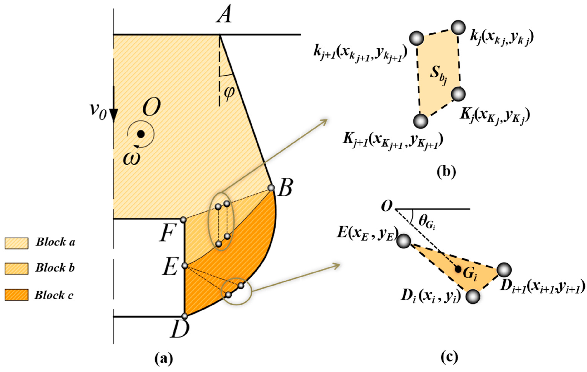
2.2. Translational–Rotational Failure Mechanism of an Underwater Shallow Square Tunnel

Within the framework of the upper bound theory, the key to accurately assessing tunnel stability is to establish a kinematically admissible failure mechanism. Therefore, a discretization technology called ‘point by point’, which was introduced by Mollon et al. to generate a rotational failure mechanism [30], has been widely adopted by many researchers to estimate the stability of geotechnical structures, as it has shown to be the most appropriate solution for Mohr–Coulomb soils [31,32,33,34,35]. By means of this discrete approach, Du et al. constructed a rotational–translational mechanism of soils around the square tunnel to compute the limit supporting pressure by using limit analysis theory [26]. Although this failure mechanism successfully incorporated the effects of soil heterogeneity and anisotropy, it ignored the velocity discontinuity surface between the upper translational block and the lower rotational block. Huang et al. have pointed out the importance of accounting for the velocity discontinuity between the translational and rotational moving blocks for the sake of having a rigorous theoretical basis and estimating an accurate solution [36].

With the combination of the aforementioned methods, an improved failure mode is proposed based on the discrete technology with velocity discontinuity surfaces between rotational and translational blocks determined numerically in this paper. The surrounding soil masses investigated are assumed to follow the Mohr–Coulomb failure criterion during the analysis.

2.2.1. Failure Mechanism Generated by the Discrete Method

The rotational–translational failure mechanism of the surrounding soil mass generated by using discretization technology for the shallow square tunnel is sketched in Figure 2a. The whole failure mechanism proposed in this paper consists of a translational rigid block $ABE{E}^{\prime }{B}^{\prime }{A}^{\prime }$ with vertically downward velocity $v_0$, and two rotational rigid blocks, namely, $BED$ and $B^{\prime }{E}^{\prime }{D}^{\prime }$ that rotate around a horizontal axis passing through the point $O$ with an angular velocity $\omega$. For any point in a rotational block, its corresponding velocity could be derived by multiplying the distance between the calculated point and the rotating center by the angular velocity. In addition, the failure zone is supposed to extend the ground (i.e., the point $A$ is located in the ground) because of the shallow tunnel involved in this paper, and the angle between line $AB$ and vertical direction is $\phi$ based on the associated flow rule.

As shown in Figure 2a, the surfaces $BD$ and $B^{\prime }{D}^{\prime }$ are discretized by a series of points with an angle $\delta \theta$, any discrete point $D_{i+1}$ could be derived from the former point $D_i$ by obeying a certain rule and ${\theta }_i$ refers to the clockwise angle between the initial direction and line $O{D}_i$ (if $i=1$, ${\theta }_i={\theta }_D$). Figure 2b illustrates that the geometric relationships of the adjacent vectors, ${\overrightarrow{n}}_i(x_{ni},y_{ni})$ denotes the unit normal vector of line $D_i{D}_{i+1}$, and ${\overrightarrow{v}}_i(x_{vi},y_{vi})$ is the unit velocity vector of point $D_i(x_i,y_i)$, thus the coordinate of unit velocity vector ${\overrightarrow{v}}_i$ $(-\sin {\theta }_i,-\cos {\theta }_i)$. Besides, the angle between vector ${\overrightarrow{v}}_i(x_{vi},y_{vi})$ and line $D_i{D}_{i+1}$ is $\phi$ because of the associated flow rule. As the relationship of vectors ${\overrightarrow{n}}_i$ and ${\overrightarrow{v}}_i$ should satisfy Equation (3), the expression of the unit normal vector ${\overrightarrow{n}}_i$ can be derived, i.e., $(\cos ({\theta }_i-\phi ),\sin (\phi -{\theta }_i))$, by substituting ${\stackrel{\rightharpoonup }{v}}_i$ into it.

$$\{\begin{array}{l}{\overrightarrow{n}}_i·{\overrightarrow{v}}_i=\cos (\frac{\pi }{2}+\phi )\\ \left|{\overrightarrow{n}}_i\right|=1\end{array}$$

(3)

Since the unit vector ${\overrightarrow{n}}_i$ is normal to the line $D_i{D}_{i+1}$, namely, ${\overrightarrow{n}}_i·\overrightarrow{D_i{D}_{i+1}}=0$, where $\overrightarrow{D_i{D}_{i+1}}$ could be replaced by $\overrightarrow{O{D}_{i+1}}-\overrightarrow{O{D}_i}$ according to Figure 2b. Furthermore, in order to simplify the calculation, $\overrightarrow{O{D}_{i+1}}$ is expressed as by ${\lambda }_{i+1}·\overrightarrow{{\delta }_{i+1}}$, where ${\lambda }_{i+1}$ is the distance between points $O(x_o,y_o)$ and $D_{i+1}(x_{i+1},y_{i+1})$, and ${\delta }_{i+1}$ refers to the unit vector $(-\cos {\theta }_{i+1},-\sin {\theta }_{i+1})$. Then, ${\lambda }_{i+1}$ could be computed as follows:

$${\lambda }_{i+1}=\frac{x_{ni}(x_i-x_o)+y_{ni}(y_i-y_o)}{x_{ni}\cos {\theta }_{i+1}-y_{ni}\sin {\theta }_{i+1}}.$$

(4)

By introducing Equation (4) into $\overrightarrow{O{D}_{i+1}}={\lambda }_{i+1}·\overrightarrow{{\delta }_{i+1}}$, the coordinate of a discrete point $D_{i+1}$ is obtained:

$$\{\begin{array}{l}{x}_{i+1}=x_o+\cos {\theta }_{i+1}·{\lambda }_{i+1}\\ y_{i+1}=y_o-\sin {\theta }_{i+1}·{\lambda }_{i+1}\end{array}.$$

(5)

Hence, with the given point $D$, the process of generating surface $BD$ can be completed based on Equation (5), as long as the position of the rotating point $O$ is determined. Likewise, the discontinuity surface $B^{\prime }{D}^{\prime }$ could also be constructed in the same way. Obviously, the accuracy of the whole failure mechanism relies on the parameter $\delta \theta$, and certainly, the smaller the $\delta \theta$, the more precise the solutions. However, too small values reduce the computational efficiency as well as have little significant effect on improving the results. Therefore, in the following analysis, this parameter is taken to be $\delta \theta ={0.1}^{\circ }$.

2.2.2. Velocity Discontinuity Surfaces $BE$ and $B^{\prime }{E}^{\prime }$

After generating the failure mechanism of the shallow square tunnel, the details of obtaining velocity discontinuity surfaces numerically will be discussed in this section. As mentioned before, the velocity vectors of any point involving the translational rigid block $ABE{E}^{\prime }{B}^{\prime }{A}^{\prime }$ and rotational rigid block $BED$ are $\overrightarrow{v_{0k}}=\overrightarrow{v_0}$ and $\overrightarrow{v_{rk}}=(\omega r_{rk}\sin {\theta }_{rk})\overrightarrow{i}-(\omega r_{rk}\cos {\theta }_{rk})\overrightarrow{j}$ (as seen in Figure 2c), where $r_{rk}$ and ${\theta }_{rk}$ refer to the distance between the point under consideration and the rotating point, and the clockwise angle between the horizontal direction and line through the calculation point and point $O$, respectively. Therefore, for any point $K(x_k,y_k)$ at the discontinuity surface, its unit tangential vector $\overrightarrow{T}$ and relative velocity vector $\overrightarrow{v_k}$ could be expressed as follows:

$$\{\begin{array}{l}\overrightarrow{T}=d{x}_k\overrightarrow{i}+d{y}_k\overrightarrow{j}\\ \overrightarrow{v_k}=\overrightarrow{v_{rk}}-\overrightarrow{v_{0k}}\end{array}.$$

(6)

Due to the assumption that the failure mechanism follows the associated flow rule, vectors $\overrightarrow{T}$ and $\overrightarrow{v_k}$ should meet the following equation, namely, $\overrightarrow{T}·\overrightarrow{v_k}=\left|\overrightarrow{T}\right|·\left|\overrightarrow{v_k}\right|·\cos \phi$. Afterwards, a differential equation that could determine the discontinuity surface $BE$ numerically can be derived:

$$(y_o-y_k)dx+(x_k-x_o+v_0)dy=\cos \phi \sqrt{{(x_k-x_o+v_0)}^2+{(y_k-y_o)}^2}.$$

(7)

By means of the function used to resolve the implicit differential equation in the software MATLAB 2019b, the numerical solutions of discontinuity surface $BE$ can be obtained on the basis of Equation (7). Similarly, another discontinuity surface $B^{\prime }{E}^{\prime }$ could also be determined. In a word, the geometry of the whole failure mechanism is totally dependent on the positions of the rotating point $O$ and point $A$.

2.3. Work Rate Calculation

In the framework of the kinematic approach of limit analysis, after generating the failure mechanism, the key to acquiring safety factors relies on calculations of the work rate of the external forces and the work rate of internal energy dissipation on the failure mechanism. External forces involved in this paper consist of soil gravity, pore-water pressure, and the supporting pressure applied on tunnel sidewalls. Energy dissipation includes dissipation within the volume and along velocity discontinuity surfaces [37]. Since the proposed failure mechanism is composed of rigid blocks, the energy dissipation rate only takes place on surfaces between adjacent rigid blocks and velocity discontinuity surfaces. As a result of the symmetry, only the half-of-failure mechanism is analyzed in this section.

2.3.1. Work Rate of Soils’ Gravity

It could be seen from Figure 3 that there may be two cases (Case 1 and Case 2) for the generation of the velocity discontinuity surface $BE$, as the various positions of point $B$, which cause different computations related to work rates.

In Case 1, as sketched in Figure 4, the total work rate of soil weight associated with the half-of-failure model could be divided into three parts, namely, the work rates of blocks $a$, $b$, and $c$. The area of a block $a$ could be easily calculated based on the geometric relationship, i.e., $S_a=S_{ABF{F}^{\prime }{B}^{\prime }{A}^{\prime }}/2$. Since the numerical result of the surface $BE$ was derived in Section 2.2.2, the total area of the block $b$ could be discretized into $n$ parts (as shown in Figure 4b), and it is considered the sum of the area related to each tiny block, i.e., $S_b={\displaystyle \sum _{j=1}^n{S}_{b_j}}$. On the other hand, for each triangular block $E{D}_i{D}_{i+1}$ involved in block $b$, its work rate of weight is as follows:

$$W_{G_{E{D}_i{D}_{i+1}}}=S_{E{D}_i{D}_{i+1}}·\omega ·O{G}_i·\cos {\theta }_{G_i}·{\gamma }_{sat},$$

(8)

where ${\gamma }_{sat}$ refers to the saturated unit weight of soil, $G_i$ is the barycenter of the block $E{D}_i{D}_{i+1}$, and ${\theta }_{G_i}$ denotes the clockwise angle between the line $O{G}_i$ and the horizontal direction (as seen in Figure 4c).

Hence, the work rate of soil weight associated with the half-of-failure model in Case 1 could be derived:

$$W_{G1}=v_0·(S_a+S_b)·{\gamma }_{sat}+{\displaystyle \sum W_G{}_{{}_{E{D}_i{D}_{i+1}}}}$$

(9)

In Case 2, it can be seen from Figure 5 that the point $E$ is located on the top wall of the tunnel. The area of a block $b$ could be thought of as the sum of $n$ triangles (see Figure 5a), so the area $S_a$ of block $a$ is $S_{ABF{F}^{\prime }{B}^{\prime }{A}^{\prime }}/2-{\displaystyle \sum _{j=1}^n{S}_{F{K}_j{K}_{j+1}}}$ and work rate $W_{F{K}_j{K}_{j+1}}$ performed by the soil weight of each block is $S_{F{K}_j{K}_{j+1}}·{\gamma }_{sat}·O{G}_j·\omega ·\cos {\theta }_{G_j}$, where $G_i$ is the barycenter of the block $F{K}_j{K}_{j+1}$ and ${\theta }_{G_j}$ represents the clockwise angle between line $O{G}_j$ and horizontal direction, as shown in Figure 5b. Apparently, the work rate $W_{F{D}_i{D}_{i+1}}$ of soil weight is $S_{F{D}_i{D}_{i+1}}·{\gamma }_{sat}·O{G}_i·\omega ·\cos {\theta }_{G_i}$. Finally, the work rate contributed by soil weight related to the half-of-failure model in Case 2 could be calculated:

$$W_{G2}=S_a·v_0·{\gamma }_{sat}+{\displaystyle \sum _{j=1}^n{W}_{F{K}_j{K}_{j+1}}}+{\displaystyle \sum _{i=1}{W}_{F{D}_i{D}_{i+1}}}.$$

(10)

2.3.2. Work Rate of Supporting Pressure

In this section, due to the square tunnel excavated underwater, studies related to work rates of supporting pressure are discussed under conditions where both water and earth pressure are considered. According to the Japanese design standard [38], the design loads acting on tunnel walls should include five parts, namely, crown loads, lateral loads on the sidewall, the dead weight of linings, the bottom loads, and lateral resisting loads. However, the deformation of linings is neglected in this analysis, so the above loads could be simplified as lateral pressure, uniform top pressure, and bottom pressure, as seen in Figure 6. It should be emphasized that the top pressure $q_1$ is considered the overburden pressure (i.e., $q_1={\gamma }_{sat}·h$). Zhang et al. stated that the lateral loads increase linearly with the depth and could be described as $e=a·y_e+e_1$ [39], where $e_1$ denotes the top pressure, which could be calculated by multiplying the top pressure $q_1$ and a lateral pressure coefficient $K_s$, and $a$ and $y_e$ refer to the gradient and depth of the computed point from the top wall. In addition, considering the resisting effect of the supporting pressure on the soil around the tunnel, the work rates of the supporting pressure should be negative.

As mentioned before, there are two different situations related to the failure mechanism that should be considered in the calculations of work rate, and only half of the model is adopted to simplify calculations because of symmetry. Therefore, for any tiny angle $d_{\theta }$ (see Figure 7b) and corresponding element on the sidewall of the tunnel in Case 1, the horizontal supporting pressure rate could be computed:

$$d{W}_{s_h}=(2e+\frac{r_{OF}·\cos {\theta }_F}{{\cos }^2\theta }·a)·\frac{r_{OF}{}^2·{\cos }^2{\theta }_F}{2{\cos }^3\theta }·\omega ·\sin \theta ·d\theta .$$

(11)

where $\theta$ represents the clockwise angle between the line through any point on the sidewall and the rotational center $O$, and the initial horizontal direction, and $r_{OF}$ is the distance between any point on the sidewall and the point $O$. Meanwhile, the work rate performed by the vertical supporting pressure is $-qb{v}_0$, where $b$ is half of the tunnel width, and then the total work rate of the supporting pressure could be derived according to Equation (11):

$$W_S=-q_{1}b{v}_0+{\displaystyle {\int }_{{\theta }_D}^{{\theta }_E}(2e+\frac{r_{OF}·\cos {\theta }_F}{{\cos }^2\theta }·a)·\frac{r_{OF}{}^2·{\cos }^2{\theta }_F}{2{\cos }^3\theta }·\omega ·\sin \theta ·d\theta }.$$

(12)

In Case 2, note that the computation of horizontal supporting pressure acting on the sidewall is similar to that in Case 1, while it should be divided into two parts for the vertical supporting pressure rate as the velocity of the surface $F_E$ is not $v_0$ (see Figure 8a). Hence, for any infinitesimal element on the crown of the tunnel with a corresponding angle $d\theta$, as illustrated in Figure 8b, the work rate of vertical supporting pressure could be obtained as follows:

$$d{W}_{S_v}=\frac{r_{OF}·\sin {\theta }_F}{{\sin }^2\theta }·q_1·\omega ·\frac{r_{OF}·\sin {\theta }_F}{\sin \theta }·\cos \theta ·d\theta .$$

(13)

Then the work rate of supporting pressure acting on the top wall of the tunnel is $-q_1{x}_o{v}_0-{\displaystyle {\int }_{{\theta }_F}^{{\theta }_E}d{W}_{S_v}}$, and the whole supporting pressure rate could be expressed according to Equation (13) in Case 2:

$$W_S=-q_1(b-x_e)v_0-{\displaystyle {\int }_{{\theta }_F}^{{\theta }_E}d{W}_{S_v}}+{\displaystyle {\int }_{{\theta }_D}^{{\theta }_F}(2e+\frac{r_{OF}·\cos {\theta }_F}{{\cos }^2\theta }·a)·\frac{r_{OF}{}^2·{\cos }^2{\theta }_F}{2{\cos }^3\theta }·\omega ·\sin \theta ·d\theta }.$$

(14)

2.3.3. Internal Energy Dissipation Rate

Based on the mentioned postulate that soil materials comply with the Mohr–Coulomb yield criterion and the associated flow rule, the tangential plastic velocity $v_s$ and the normal plastic velocity $v_n$ on the failure surface should satisfy Equation (15) for the reason that the plastic potential surface coincides with the yield surface, namely, $\mathit{\psi }=\mathit{G}$. Where $\mathit{G}$ refers to the yield function, and it could be written as $\mathit{G}(\sigma ,\tau )=\tau -c-\sigma \tan \phi$.

$$\frac{v_n}{v_s}=\frac{\partial \psi /\partial \sigma }{\partial \psi /\partial \tau }=\frac{\partial G/\partial \sigma }{\partial G/\partial \tau }=-\tan \phi$$

(15)

Equation (15) shows that, for any point located on the failure surface included in the soil masses discussed, the angle between its plastic velocity and the failure surface is $\phi$. Since the internal energy dissipation rate along the failure surfaces could be computed as the product of internal force and plastic velocity, the energy dissipation over the unit velocity discontinuity surface is the following:

$$dD=\tau v_s+\sigma v_n=(\tau \cos \phi -\sigma \sin \phi )v=c\cos \phi v.$$

(16)

As previously mentioned, collapsing blocks are assumed to be rigid, and energy dissipation only occurs on velocity discontinuity surfaces $CD$, $BC$, and $AC$. The surfaces $BE$ and $BD$ could be divided into a finite number of linear element $K_j{K}_{j+1}$ and $D_i{D}_{i+1}$, respectively. Corresponding energy dissipations along the tiny element are $c·v_j·L_j·\cos \phi$ and $c·\omega ·R_i·L_i·\cos \phi$, where $v_j$ is the relative velocity of the center point of the line $K_j{K}_{j+1}$. $R_i$ is the distance from the rotational center $O$ to the center point of line $D_i{D}_{i+1}$. $L_j$ and $L_i$ represent the length of elements $K_j{K}_{j+1}$ and $D_i{D}_{i+1}$, respectively. In addition, the energy dissipation of the surface $AB$ is straightforward, namely, $c·v_0·AB·\cos \phi$; therefore, the total internal energy dissipation of the proposed failure mechanism is the following:

$$D={\displaystyle \sum _{j=1}^{n}c·v_j·L_j·\cos \phi }+{\displaystyle \sum _{i=1}c·\omega ·R_i·L_i·\cos \phi }+c·v_0·AB·\cos \phi .$$

(17)

Basically, there are two effective methods to define safety factors: the strength reduction technique and the ratio of the load-resisting capacity to the externally destructive effect [33,40], namely, $FS=(D-W_S)/(W_U+W_G)$. The second approach is adopted in the present analysis since it is more computationally efficient and can explicitly obtain the safety factor. Thus, by combining Equations (11), (12), (14), (16), and (17), the safety factor can be expressed as:

$$FS=\{\begin{array}{l}\frac{(b{v}_0+0.5\omega K_s{r}_{OF}{}^2({\tan }^2{\theta }_E-{\tan }^2{\theta }_D))q_1+D}{{\gamma }_{sat}(v_0(0.5((x_a+x_b)(-y_b)+(b+x_b)(C+y_b))+{\displaystyle \sum _{j=1}^n{S}_{b_j}})+W_{G_c}+W_U} (Case 1)\\ \frac{((b-x_e)v_0+0.5\omega K_s{r}_{OF}{}^2(({\cot }^2{\theta }_F-{\cot }^2{\theta }_E)+({\tan }^2{\theta }_F-{\tan }^2{\theta }_D)))q_1+D}{{\gamma }_{sat}(v_0(0.5((x_a+x_b)(-y_b)+(b+x_b)(C+y_b))+{\displaystyle \sum _{j=1}^n{S}_{b_j}})+W_{G_c}+W_U} (Case 2)\end{array}$$

(18)

where $W_U$ is the work rate performed by the pore-water pressures. Equation (18) shows that supporting pressure $q$ only depends on the values of ${\theta }_D$, ${\theta }_F$, and $x_a$, in other words, the whole failure mechanism could be determined uniquely by the aforementioned three parameters. The critical value of supporting pressure could be searched by utilizing the optimization function called Particle Swarm in MATLAB 2019b, in which ${\theta }_D$, ${\theta }_F$, and $x_a$ are optimizing variables, and their values should follow Equation (19). Nevertheless, the only item $W_U$ is unknown, which is derived by means of the conformal mapping method and is discussed in Section 2.4.

$$\{\begin{array}{l}\frac{\pi }{2}-{\theta }_F>0\\ \frac{\pi }{2}-{\theta }_D>0\\ x_a>0\end{array}$$

(19)

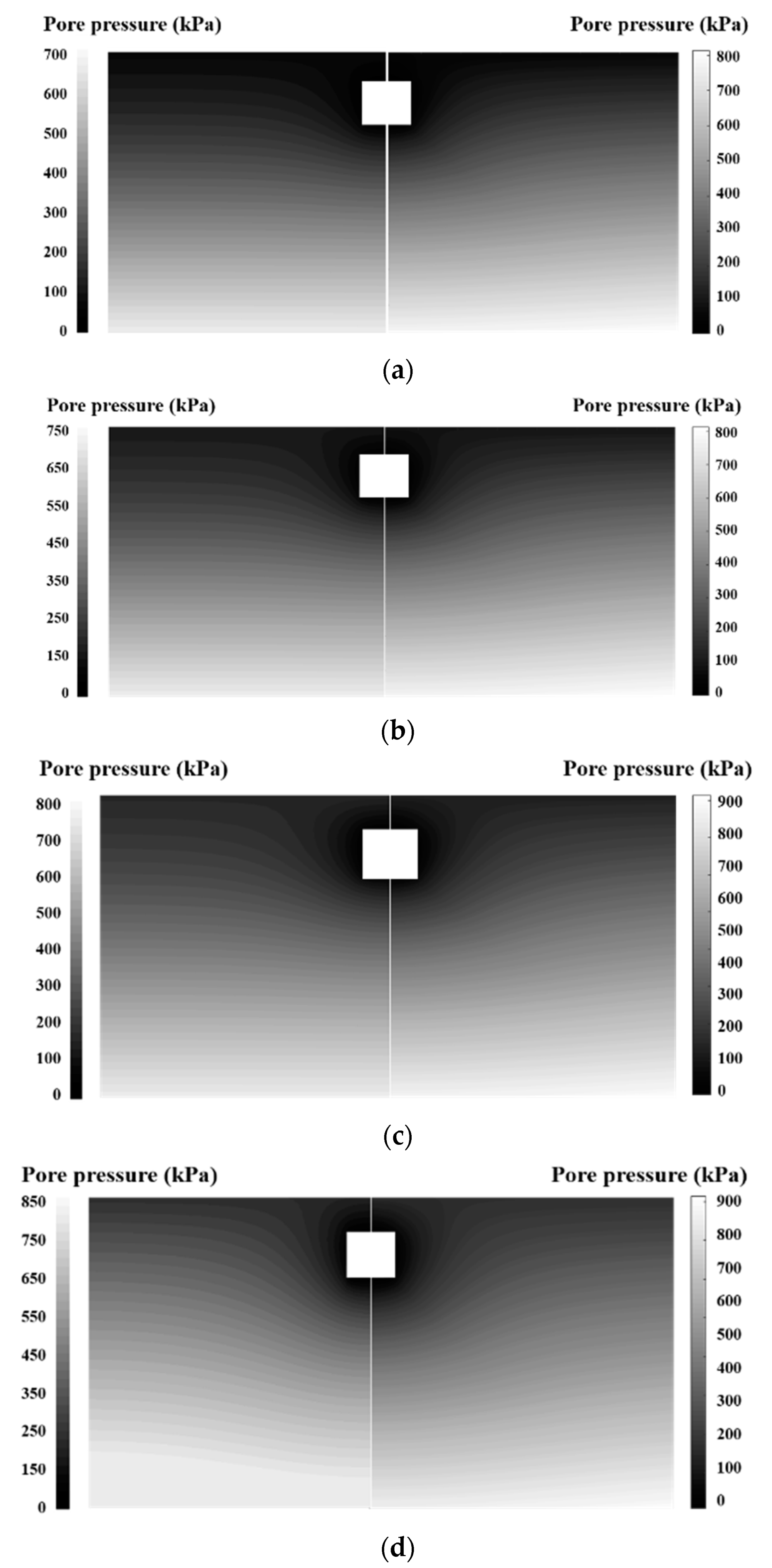
2.4. Analytical Solutions of Pore-Water Pressure Distribution around Tunnels

To obtain actual pore-water pressure distributions, analytical solutions of the pore-water pressure field around tunnels have been elucidated [41,42]. However, the focus of these studies was on circular tunnels. Since the boundary conditions of a square tunnel are highly complicated, studies on pore-water pressure distributions around square tunnels are limited. This section narrowed this gap.

This section will first map the original plane onto the image plane by using the conformal mapping technique. Such a procedure can simplify the complex seepage domain to the rectangle domain. Then, the Laplace equation in the form of a potential function $\phi (x,y)$ can be solved in the image plane based on the boundary conditions of square tunnels. Finally, to obtain the pore-water pressure distributions around square tunnels, the analytical solutions on the image plane will be transformed back to the original plane. Note that in the analysis, the shear strength parameters of dry soils are the same as those under the water table.

2.4.1. Conformal Mapping

According to Darcy’s law and the law of mass conservation, the Laplace equation in the two-dimensional steady-state groundwater flow around the tunnels can be described using the equation reported by [42], as follows:

$$\frac{{\partial }^2\phi }{\partial x^2}+\frac{{\partial }^2\phi }{\partial y^2}=0.$$

(20)

With

$$\phi (x,y)=\phi (z)=-kH=-k(y+p/{\gamma }_w),$$

(21)

where $k$ is the permeability coefficient, $H$ is the hydraulic head, $p$ is the pore-water pressure, and ${\gamma }_w$ is the bulk density of water.

Based on the conformal transformation, the flow domain in the original $z$-plane is mapped conformally onto a rectangle in the $\zeta$-plane as shown in Figure 9a–d. The potential function can be solved in the $\zeta$-plane, and the solution can be transferred to the $z$-plane. The following sections will elaborate on how to achieve conformal mapping from the $z$-plane to the $\zeta$-plane for the flow domain.

The fractional linear transformation is [43]:

$$\omega =u+iv=\frac{z+i\sqrt{{(h+b)}^2-b^2}}{z-i\sqrt{{(h+b)}^2+b^2}}.$$

(22)

According to Equation (22), the ground surface and the circumference of square tunnels in the $z$-plane can be mapped conformally onto a semicircle with a radius of 1 and a non-circular shape in the $\omega$-plane, respectively. The non-ring-shaped region is denoted by $S$, see Figure 9b.

The key to achieving the transformation shown in Figure 9b,c is to define the specific mapping function $\pi =f(\omega )$. Many researchers have derived mapping functions using different polygons to approximate tunnel shapes [44,45], but this method has low precision. To overcome this, Lu and Wang used the complex method proposed by Box to derive the mapping function that can map a tunnel of arbitrary shape onto a circle of radius 1 [46,47]. In this study, to map the region S in the $\omega$-plane into a ring bounded by the circles $\left|\pi \right|=1$ and $\left|\pi \right|=r_s$ in the $\pi$-plane, where $r_s>1$ (see Figure 9c), a modified complex method is adopted to obtain $\pi =f(\omega )$ [48]. Compared to the method proposed by Box [46], this method overcame the drawbacks of a relatively slow convergence rate that requires many iterations.

The inverse function $\omega =f(\pi )$ of the function $\pi =f(\omega )$ can be expanded using the Laurent series:

$$\{\begin{array}{l}\omega =f(\pi )=R\left(\pi +{\displaystyle \sum _{k=0}^n{C}_k}{\pi }^{-k}\right)\\ \omega =r_j{e}^{i\alpha }, \pi =\rho e^{i\beta }\end{array},$$

(23)

where $R$ is a positive real number, $C_k$ is the real number due to symmetric conditions, $k=0,1,2, \dots ,n$ ($n$ refers to the positive integer).

Because the tunnel circumference in the $\omega$-plane corresponds to the unit semicircle in the $\pi$-plane, Equation (23) can be rewritten as:

$$r_j{e}^{i{\alpha }_j}=R_1\left(e^{i{\beta }_j}+{\displaystyle \sum _{k=0}^n{C}_k{e}^{-ik{\beta }_j}}\right).$$

(24)

By separating the imaginary part from the real part of Equation (24), two formulas for obtaining the mapping function are derived:

$$\{\begin{array}{l}B{B}_j\cos {\alpha }_j-A{A}_j\sin {\alpha }_j=0\\ r_j=R_1(A{A}_j\cos {\alpha }_j+B{B}_j\sin {\alpha }_j)\end{array}.$$

(25)

where $A{A}_j$ and $B{B}_j$ can be defined separately as:

$$\{\begin{array}{l}A{A}_j=C_0+\cos {\beta }_j+{\displaystyle \sum _{k=1}^n{C}_k}\cos (k{\beta }_j)\\ B{B}_j=\sin {\beta }_j-{\displaystyle \sum _{k=1}^n{C}_k}\sin (k{\beta }_j)\end{array}.$$

(26)

Note that the items $R_1$ and $C_k$ of Equations (25) and (26) are the key to obtaining the mapping function of the tunnel circumference, which will be derived next.

As shown in Figure 10, $m_1+1$ points ($0$ to $m_1$) along the boundary of tunnels at the $u$-axis counterclockwise are selected in the $\omega$-plane, and any point $A_j(1,{\alpha }_{jj})$ in the $\omega$-plane can be mapped onto the corresponding point $a_j{}^{\prime }(1,{\beta }_j)$ in the $\pi$-plane. It is assumed that the coordinate point $a_0(r_0,0)$ can be precisely mapped onto the corresponding point $a_0{}^{\prime }(1,0)$ and ${\alpha }_0={\beta }_0=0$ ($j=0$). The relationship between $R_1$ and $C_k$ can therefore be derived according to Equation (24):

$$R_1=\frac{r_0}{1+{\displaystyle \sum _{k=0}^n{C}_k}}.$$

(27)

Note that $R_1$ can be derived by determining the expansion term $C_k$ of the Laurent series because $r_0$ is known in advance. To obtain the value of $C_k$, the modified complex method is adopted, and the objective function $f_1$ for optimization can be expressed as:

$$f_1={{\displaystyle \sum _{j=1}^{m_1}\left[r_j-R_1(A{A}_j\cos {\alpha }_j+B{B}_j\sin {\alpha }_j)\right]}}^2.$$

(28)

The optimal value of $C_k$ corresponds to the minimum $f_1$. Then the mapping function that maps the tunnel circumference onto the unit semicircle can be derived from Equation (23).

Apparently, a point $A_j$ at the ground surface in the $\omega$-plane can be mapped accurately onto a point $A_j{}^{\prime }$ in the $\pi$-plane accurately, therefore, Equation (23) can be rewritten as follows:

$$e^{i\alpha {\alpha }_j}=R_2\left(r_s{e}^{i\beta {\beta }_j}+{\displaystyle \sum _{k=0}^n{C}_k{r}_s{}^{-k}{e}^{-ik\beta {\beta }_j}}\right).$$

(29)

By separating the imaginary part from the real part of Equation (29), two formulas for determining the mapping function that maps the ground surface from the $\omega$-plane to the $\pi$-plane can be derived as:

$$\{\begin{array}{l}D{D}_j\cos \alpha {\alpha }_j-C{C}_j\sin \alpha {\alpha }_j=0\\ 1=R_2(C{C}_j\cos \alpha {\alpha }_j+D{D}_j\sin \alpha {\alpha }_j)\end{array}.$$

(30)

where $C{C}_j$ and $D{D}_j$ are the intermediate variables, they can be expressed as:

$$\{\begin{array}{l}C{C}_j=C_0+r_s\cos (\beta {\beta }_j)+{\displaystyle \sum _{k=1}^n{C}_k}\cos (k\beta {\beta }_j)/r_s{}^k\\ D{D}_j=r_s\sin \beta {\beta }_j-{\displaystyle \sum _{k=1}^n{C}_k}\sin (k\beta {\beta }_j)/r_s{}^k\end{array}.$$

(31)

Similar to the method for deriving the mapping function that maps the ground surface from the $\omega$-plane to the $\pi$-plane, the mapping function that maps the boundary of tunnels can be determined as follows:

As shown in Figure 11, $m_2+1$ points ($0$ to $m_2$) along the ground surface at the $u$-axis counterclockwise are selected in the $\omega$-plane, and any point $A_j(1,{\alpha }_{jj})$ in the $\omega$-plane can be mapped onto the corresponding point $A_j{}^{\prime }(r_s,\beta {\beta }_j)$ in the $\pi$-plane. It is assumed that the coordinate point $A_0(1,0)$ can be mapped onto the point $A_0{}^{\prime }(r_s,0)$ in the $\pi$-plane and $\alpha {\alpha }_0=\beta {\beta }_0=0$ ($j=0$). Thus, $R_2$ can be obtained according to Equation (24):

$$R_2=\frac{1}{r_s+{\displaystyle \sum _{k=0}^n{C}_k{r}_s{}^{-k}}}.$$

(32)

To determine $R_2$, $C_k$, and $r_s$, an objective function $f_2$ for optimization is defined as:

$$f_2={{\displaystyle \sum _{j=1}^{m_2}\left[1-R_2(C{C}_j\cos \alpha {\alpha }_j+D{D}_j\sin \alpha {\alpha }_j)\right]}}^2.$$

(33)

The optimal value of $C_k$ and $r_s$ corresponds to the minimum value of $f_2$. Next, the mapping function that maps the ground surface can be derived from Equation (23). As using Equation (28) or Equation (33) individually to obtain the mapping function will reduce the mapping accuracy, an objective function $f$ for optimization to obtain the value of $C_k$ and $r_s$ should be constructed [47].

$$f={{\displaystyle \sum _{j=1}^{m_1}\left[r_j-R_2(A{A}_j\cos {\alpha }_j+B{B}_j\sin {\alpha }_j)\right]}}^2+{{\displaystyle \sum _{j=1}^{m_2}\left[1-R_2(C{C}_j\cos \alpha {\alpha }_j+D{D}_j\sin \alpha {\alpha }_j)\right]}}^2$$

(34)

Since the excessive Laurent series expansion terms in Equation (34) will cost much time and have no obvious effect on the improvement of mapping accuracy, only the minimum Laurent series expansion terms that can satisfy the precision requirement are determined. Lu found that the mapping accuracy can be satisfied when the number $n$ of Laurent series expansion terms is 3 [47]. Therefore, the value of $C_k$ ($C_1$, $C_2$, and $C_3$) and $r_s$ corresponding to the minimum value of $f$ are considered to be the optimal solution. The inverse function $\omega =f(\pi )$ can be obtained by taking the optimal solution into Equation (23). There are two constraints to highlight:

$$\{\begin{array}{l}{\displaystyle \sum _{k=1}^{n}k\left|C_k\right|}<1\\ r_s>1\end{array}.$$

(35)

Based on Equations (22) and (23), the tunnel boundary and ground surface in the $z$-plane can be mapped precisely onto the $\pi$-plane by Equation (36).

$$\pi =F(z)$$

(36)

$$\zeta =\xi +i\eta =\ln \pi =\ln (\epsilon +i\phi )$$

(37)

By means of the logarithm transformation (i.e., Equation (37)), the half-concentric circle with radius 1 and $r_s$ can be mapped onto a rectangle [42]. By substituting Equation (36) into Equation (37), the mapping relationship from the $z$-plane onto the $\zeta$-plane can finally be obtained:

$$\zeta =\xi +i\eta =\ln (F(z))=f(z)=f(x,y).$$

(38)

2.4.2. Solutions for Pore-Water Pressure Distribution

Using the method described in Section 2.4.1, the pore-water pressure $p^{\prime }(\xi ,\eta )$ under conditions where gravity is neglected can match the Laplace equation in the $\zeta$-plane, i.e., $({\partial }^2{p}^{\prime }/\partial {\xi }^2)+({\partial }^2{p}^{\prime }/\partial {\eta }^2)=0$, and it can be described as:

$$p^{\prime }(\xi ,\eta )=p_e+\frac{p_e-p_w}{{\xi }_e-{\xi }_w}(\xi -{\xi }_e),$$

(39)

where $p_e$ and $p_w$ refer to the pore-water pressure at the ground surface and along the tunnel circumference, respectively, as shown in Figure 12. By returning Equation (39) to the $z$-plane, it can be rewritten as (the boundary condition of zero water pressure along the tunnel circumference $p_w=0$ is assumed in this study):

$$p^{\prime }(x,y)=h_w·{\gamma }_w+\frac{h_w·{\gamma }_w}{\ln r_s}(G(x,y)-\ln r_s),$$

(40)

where $G(x,y)$ is the real part of the function $f(x,y)$, i.e., $G(x,y)=\mathrm{Re}(f(x,y))$, see Equation (38).

However, the assumption that gravity is neglected for $p^{\prime }(x,y)$ is not academic. Therefore, functions $X(x,y)$ and $Y(x,y)$ determined by the boundary conditions are introduced to consider the influence of the bulk density ${\gamma }_w$ and elevation $y$ [42]. Hence, the realistic pore-water pressure $p(x,y)$ can be derived as:

$$p(x,y)=h_w·{\gamma }_w+X(x,y)+\frac{h_w·{\gamma }_w+Y(x,y)}{\ln r_s}(G(x,y)-\ln r_s).$$

(41)

In the case of $x\to \infty$, $G(x,y)\to \ln r_s$ and the pore-water pressure $p(x,y)$ relies on the elevation $y$, i.e., $p(x,y)=h_w-y·\gamma$. Thus, Equation (41), in the case of $x\to \infty$, can be simplified as:

$$p(x,y)=h_w-y·\gamma =h_w·\gamma +X(x,y) (x\to \infty ).$$

(42)

The seepage domain could be divided into three parts along the connecting line between the inflection point and center of the square tunnel, and then Equation (41) can be expressed:

$$p(x,y)=p_w=X(x,y)-Y(x,y)\{\begin{array}{l}y>x-h-b\\ -x-h+b\le y\le x-h-b\\ y<-h+b\end{array}.$$

(43)

In the boundary condition of the tunnel circumference, as pore-water pressure $p_w$ is zero and $G(x,y)=0$. $X(x,y)$, and $Y(x,y)$ can be derived by combining Equations (42) and (43):

$$X(x,y)=-y·{\gamma }_w ,$$

(44)

$$Y(x,y)=\{\begin{array}{l} h·{\gamma }_{w }\hspace{1em}\hspace{1em}\hspace{1em}\hspace{1em}\hspace{1em}\hspace{1em}\hspace{1em}\hspace{1em}\hspace{1em}\hspace{1em}\hspace{1em}\hspace{1em}\hspace{1em}\hspace{1em} (y>x-h-b)\\ {\gamma }_w·\left(b·\tan \left(\arcsin \left(\frac{y+h+b}{\sqrt{x^2+{(y+h+b)}^2}}\right)\right)-h-b\right) (-x-h+b\le y\le x-h-b)\\ (-h-2b)·{\gamma }_w\hspace{1em}\hspace{1em}\hspace{1em}\hspace{1em}\hspace{1em}\hspace{1em}\hspace{1em}\hspace{1em}\hspace{1em}\hspace{1em}\hspace{1em} (y<-h+b)\end{array}$$

(45)

By substituting Equations (44) and (45) into Equation (41), the analytical solution of pore-water pressure can be expressed as shown below:

$$p(x,y)=h_w·{\gamma }_w-y·{\gamma }_w+\frac{h_w·{\gamma }_w-Y(x,y)}{\ln r_s}·\left(G(x,y)-\ln r_s\right).$$

(46)

2.4.3. Work Rates Performed by the Pore-Water Pressures

As elaborated in Viratjandr and Michalowski [29], under conditions where the presence of pore-water pressure is taken into account in the kinematic analysis, its work rates can be formulated as a sum of the work rates of pore-water pressure on the skeleton expansions and boundaries, i.e., the following:

$$W_U={\displaystyle {\int }_V\underset{Seepage force}{\underbrace{-{\gamma }_w·\frac{\partial h}{\partial x_i}}}·}{v}_{i}dV·+{\displaystyle {\int }_V\underset{Buoyancy forcce}{\underbrace{{\gamma }_w·\frac{\partial Z}{\partial x_i}}}}·v_{i}dV=-{\displaystyle {\int }_{V}u}·{\epsilon }_{ii}dV-{\displaystyle {\int }_{S}u}·n_i·v_{i}dS,$$

(47)

where ${\gamma }_w$ refers to the unit weight of water, $h$ denotes the hydraulic head, and $Z$ represents the elevation head. Since the collapsing blocks are assumed to be rigid, the volumetric strain in this equation can be neglected. Thus, the work rate $W_U$ contributed by pore-water pressures can be expressed by the following:

$$W_U=-{\displaystyle {\int }_{S}u·n_i}·v_{i}dS.$$

(48)

To compute the work rate of pore-water pressure, a discretized scheme is utilized on the surface $AB$, which is uniformly divided into $n_k$ parts along the vertical direction (see Figure 13), and as mentioned in Section 2.2, surfaces $BE$ and $BD$ consist of plenty of discrete elements. Hence, according to Equation (47), the work rate of pore-water pressure on each part can be computed as the product of pore-water pressure at the midpoint, the length of each part, and the vertical component of velocity at the midpoint. The work rates $W_{U_{i,i+1}}$, $W_{U_{j,j+1}}$, and $W_{U_{k,k+1}}$ of pore-water pressure on $D_i{D}_{i+1}$, $K_j{K}_{j+1}$, and $A_k{A}_{k+1}$ can be expressed as:

$$\{\begin{array}{l}{W}_{U_{i,i+1}}=p_{i+1/2}·D_i{D}_{i+1}·v_{r_i}·\sin \phi \\ W_{U_{j,j+1}}=p_{j+1/2}·K_j{K}_{j+1}·v_j·\sin \phi \\ W_{U_{k,k+1}}=p_{k+1/2}·A_k{A}_{k+1}·v_0·\sin \phi \end{array},$$

(49)

where $D_i{D}_{i+1}$, $A_k{A}_{k+1}$, and $K_j{K}_{j+1}$ are the discretized elements of the surfaces $BD$, $AB$, and $BE$, respectively. Where $v_{r_i}$ and $v_j$ refer to the linear velocity of midpoint $D_{i+1/2}$ at the element $D_i{D}_{i+1}$, and the relative velocity of midpoint $K_{j+1/2}$ at the element $K_j{K}_{j+1}$; $p_{i+1/2}$, $p_{k+1/2}$, and $p_{j+1/2}$ are the pore-water pressures located at the midpoints of surfaces $D_i{D}_{i+1}$, $A_k{A}_{k+1}$, and $K_j{K}_{j+1}$. Therefore, the total work rates achieved by pore-water pressures can be obtained:

$$W_U=\sin \phi ({\displaystyle \sum _{i=1}{p}_{i+1/2}·D_i{D}_{i+1}·v_{r_i}}+{\displaystyle \sum _{k=1}^{n_k}{p}_{k+1/2}·A_k{A}_{k+1}·v_0}+{\displaystyle \sum _{j=1}{p}_{j+1/2}·K_j{K}_{j+1}·v_j}).$$

(50)

Finally, the safety factors of square tunnels in a water-bearing zone are obtained by substituting the work rates of the pore-water pressure into Equation (18).

3. Verification

3.1. Verification in Terms of Pore-Pressure Distributions

In order to prove the rationality of the solutions, the pore-water pressure distributions, safety factors, and failure mechanisms obtained by the presented method have been compared with the results using the finite difference software FLAC3D 6.0. Due to the symmetry of the tunnel section, only half of the domain is modeled. The considered numerical model contains approximately 8000 zones and 12,378 nodes. The dimensions of the model are taken as 150 m in the X direction, 1 m in the Y direction, and 80 m in the Z direction (see Figure 14). The dimension of the numerical model is set to be much smaller in the Y direction than in the X and Z directions due to the two-dimensional problem discussed in this paper. It should be noted that the process of hydromechanical analysis with FLAC3D 6.0 can be divided into three steps: (1) the mechanical-only calculation, during which the numerical model is cycled to equilibrium to obtain an initial ground stress field before tunnel excavation; (2) the fluid flow-only calculation during the tunnel excavation to derive the pore-water pressure distributions in the soil mass surrounding the tunnel; and (3) the mechanical-only calculation is conducted to calculate the safety factor of excavated tunnels. In the numerical simulation, both mechanical boundary conditions and hydraulic boundary conditions need to be emphasized. For the mechanical boundary conditions, the displacements at the bottom of the numerical model are fixed, and displacements in the normal direction are fixed for the other vertical boundaries. For the hydraulic boundary conditions, the pore-water pressure at the tunnel perimeter is assumed to be zero, and the pore-water pressure at the water surface is fixed to be zero for the steady-state fluid flow analysis. Soil masses obey the Mohr–Coulomb failure criterion. Bulk modulus and shear modulus are set to 120 MPa and 45 MPa, respectively. The other parameters are $K$ = 1, $c$ = 25 kPa, ${\gamma }_{sat}$ = 20 kN/m³, $\phi$ = 20°, $h$ = 10.0 m, $b$ = 5.0 m, $p_w$ = 0, and $k$ = 5 × 10⁻¹² m/s.

Comparisons of the pore-water pressure distributions are shown in Figure 15. It can be seen that the pore-water pressure contours obtained by this work are well accorded with those obtained by FLAC3D 6.0. Thus, the analytical solution of pore-water pressure derived in Section 2.4.3 can well describe the actual pore-water pressure distributions around square tunnels. The value of the pore-water pressure at each point selected on the velocity-discontinuity surfaces of the failure mechanism can be obtained precisely and then calculated (results) using the first approach mentioned in Section 2.3.3. It is clear from these plots that the lower pore-water pressure around the surface and tunnel is lower due to the presence of a free surface, and the pore-water pressure contour around the square tunnel is similar to horseshoe-shaped. With the increase in water heights, the horseshoe shape will get bigger, and the pore pressure will obviously increase.

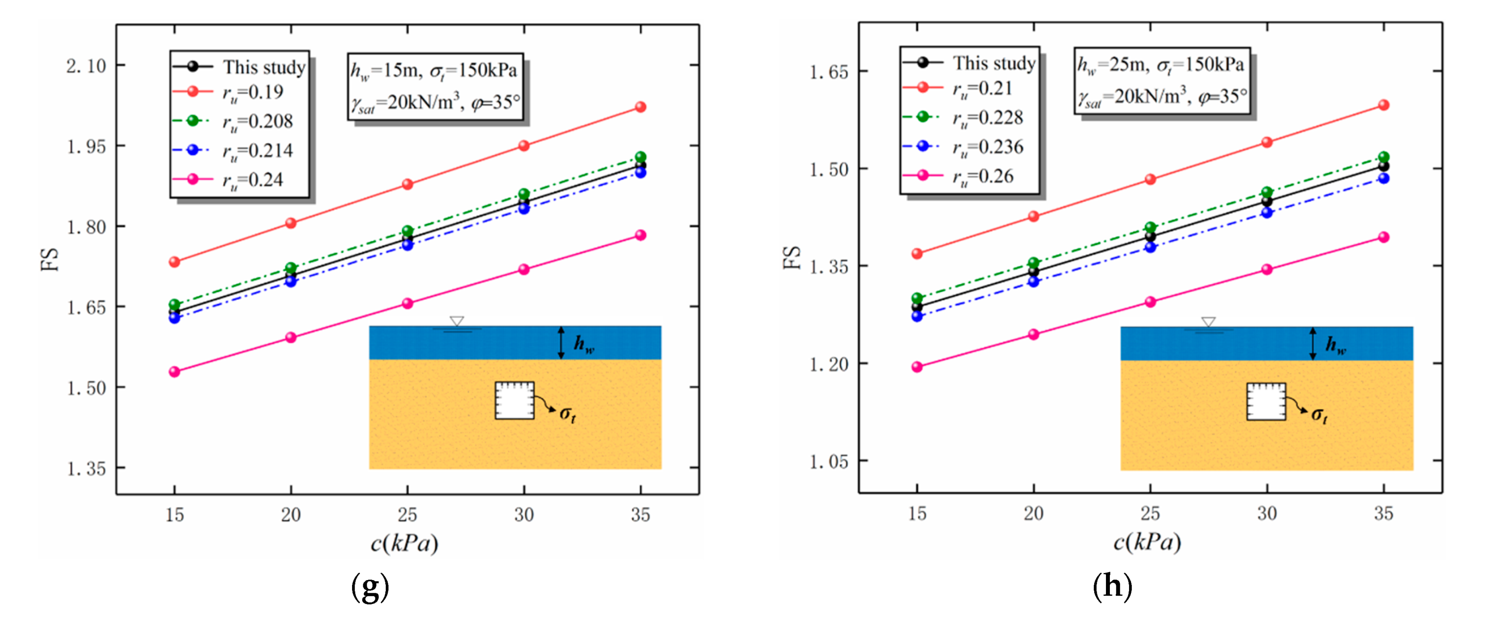
3.2. Verification in Terms of Existing Solutions

A comparison between the presented work and the results computed by Du et al. [26] was presented in this section to evaluate the accuracy of the proposed approach. It should be stated that the failure mechanism that Du et al. [26] established using the discrete method is a classical model for stability assessment of the shallow square tunnel, where the results corresponding to the ultimate limit state are presented in the form of supporting pressure ${\sigma }_t$. To perform the comparisons, the supporting pressures computed by Du et al. [26] are adopted as input parameters to the proposed model to judge whether the obtained safety factors are close to one or not. The results of the comparisons mainly include the dry soil and saturated soil conditions, which are presented in

Table 2. Comparisons with existing solutions.

Case	$\mathit{c}$ (kPa)	$\mathit{\phi }$ (degrees)	${\mathit{r}}_{\mathit{u}}$	Du et al. [26]	This Study	Difference (%)
				${\mathit{\sigma }}_{\mathit{t}} \mathbf{Corresponding} \mathbf{to} \mathbf{FS} = 1.0$ (kPa)	Safety Factor (FS)
Dry soil condition	10	15	/	186.4 (FS = 1)	0.946	5.4
		18	/	158.3 (FS = 1)	0.980	2.0
		21	/	135.0 (FS = 1)	1.045	4.5
		24	/	114.3 (FS = 1)	1.105	10.5
Saturated soil	20	18	0.40	158.2 (FS = 1)	1.161	16.1
			0.45	156.4 (FS = 1)	1.156	15.6

. Additionally, the water table is at the surface in the saturated soil condition, corresponding to the case of $h_w$ = 0 involved in this paper. The corresponding parameters are as follows: $\gamma$ = 20 kN/m³ (dry soil condition), ${\gamma }_{sat}$ = 20 kN/m³ (saturated soil condition), $h$ = 20 m, $b$ = 5 m, and $K$ = 1.

It can be observed that, for the dry condition, the safety factors evaluated by this work are very close to one, and the maximum difference only equals 10.5%, whereas the differences between the results and one are a little bigger than the former case in the saturated soil condition, with a maximum difference of 16.1%. The reason for such a difference may be that the pore-water coefficient method cannot accurately consider the actual effect of pore-water pressure on the failure mechanism, which will be discussed in more detail in the next section. In general, the differences in all cases are acceptable, which further validates that the proposed method is applicable to the stability analysis of underwater square tunnels. Note that the computed safety factors will decrease with the increase of pore-water coefficients, which means that the selection of pore-water pressure coefficients has an important impact on the stability assessment of tunnels under seepage flow conditions.

4. Comparisons and Discussion

To simplify calculations of pore-water pressure, Bishop and Morgenstern [27] assumed that pore-water pressure is only related to depth by defining a pore pressure coefficient $r_u$. However, in practical application, the pore-water pressure of a specific point is not only related to the vertical distance from the point in the soil to the water table elevation but also to the horizontal distance and the boundary conditions of tunnels. For these reasons, the solutions computed by this simplified method are satisfactory only when the value of the pore pressure coefficient is reasonable, and the pore pressure coefficient is usually determined based on engineering experience. Thereby, the effect of pore-water pressures on the stability of saturated square tunnels cannot be accurately analyzed by the simplified method.

To illustrate the limitations of the simplified approach further, some pore pressure coefficients are chosen to compute the safety factors based on the proposed failure mechanism. Moreover, the obtained results are compared with the solutions calculated by the proposed approach in this section. The results are plotted in Figure 16, where the input parameters are as follows: $K$ = 1, $h$ = 15.0 m, $b$ = 5.0 m, $p_w$ = 0, and $k$ = 5 × 10⁻¹² m/s.

Figure 16 shows that the effect of the pore pressure coefficient on the stability of tunnels is significant in all cases. Additionally, it is difficult to choose a reasonable pore pressure coefficient to derive a solution that agrees well with that in the practical condition. For instance, in the case of $\phi =20°$ and $h_w=15 \mathrm{m}$, the safety factors with $r_u=0.25$ are much higher than the presented results, yet the solutions with $r_u=0.32$ are much lower than the safety factors computed by the proposed approach. In addition, it should be noted that for each case in Figure 16, an appropriate range of pore pressure coefficients to obtain solutions consistent with practical results can be found. For example, in the case of $\phi =20°$ and $h_w=25 \mathrm{m}$, the results with $r_u=0.295$ and $r_u=0.312$ are a little higher and lower than the presented solutions, respectively, as shown in Figure 16b. Meantime, it can be seen from Figure 16a,c,e, and g that, with the increase of the friction angles of soil, the pore pressure coefficients that lead to solutions close to the presented results will decrease, and the increase of water heights will result in an increase in pore pressure coefficients. It suggests the following: (a) in the case of constant water table elevations, using constant pore pressure coefficients to compute safety factors of tunnels in soils with different friction angles give rise to inaccurate results; (b) the influence of water table elevations should also be taken into consideration in the selection of pore pressure coefficient. In summary, although defining the pore pressure coefficient to compute pore-water pressure can simplify the seepage flow problems, it needs a reasonable pore-water pressure coefficient that considers the effects of water table elevation $h_w$, friction angle $\phi$ and cohesion $c$. Given this, this section provides a reasonable prior range of pore pressure coefficients for practical use, which can improve accuracy when using the simplified method.

After plenty of computations, a design table (see

Table 3. Reference values of pore-water pressure coefficients.

Case	$\mathit{\phi }$ (degree)	${\mathit{h}}_{\mathit{w}} \left(\mathbf{m}\right)$	$\mathit{c}$ (kPa)	$\mathbf{Maximum} \mathbf{Value} \mathbf{of} {\mathit{r}}_{\mathit{u}}$	$\mathbf{Minimum} \mathbf{Value} \mathbf{of} {\mathit{r}}_{\mathit{u}}$
1	20	15	15~35	0.275	0.290
2	20	25	15~35	0.295	0.312
3	25	15	15~35	0.252	0.264
4	25	25	15~35	0.274	0.282
5	30	15	15~35	0.231	0.238
6	30	25	15~35	0.250	0.258
7	35	15	15~35	0.208	0.214
8	35	25	15~35	0.228	0.236

) that facilitates geotechnical designers in choosing a reasonable pore pressure coefficient to estimate the stability of tunnels considering the effects of pore-water pressures is presented. Table 3 includes a total of eight cases, corresponding to the soil with four different friction angles ($\phi =20°,25°,30°$ and $35°$) under two water heights ($h_w$ = 15 m and 25 m). For each case, the cohesion varies from 15 kPa to 35 kPa, the depth $h$ of the tunnel center from the ground surface is set to 15 m, the supporting pressure is set to 150 kPa, and the saturated unit weight ${\gamma }_{sat}$ of soil is set to 20 kN/m³. As can be seen in Table 3, geotechnical designers can select a suitable value from the range of pore pressure coefficients given in Table 3 in advance.

5. Conclusions

Existing kinematical approaches to limit analysis have the following drawbacks: (1) using an empirical approach that cannot reflect the realistic pore-water pressure field around tunnels to estimate pore-water pressure distribution; (2) adopting a failure mechanism that is not rigorously kinematically admissible. Thus, to overcome these limitations, we present a kinematically admissible rotational–translational failure mechanism considering a possible variation of discontinuity velocity surfaces between translational and rotational blocks and acquire pore-water pressure distributions around tunnels so as to investigate the stability of a submerged shallow square tunnel. The analytical solution of pore-water pressure employing the conformal mapping of the complex variable methods is formulated, and then a linear interpolation technique is proposed to calculate the pore-water pressure of the point on the presented failure mechanism. Work rates attributed to pore-water pressures, soil weight, and internal dissipation rates are computed to explicitly obtain the safety factor of shallow square tunnels in water-bearing zones.

The proposed model is validated in terms of pore-water pressure distributions and safety factors by comparing it with the numerical software FLAC3D 6.0 and existing solutions. Compared to numerical simulation, the computational cost of using the proposed model can be reduced by 98.3%. Comparisons between the results calculated by the proposed method and the simplified method demonstrate the following: (i) The effect of the pore pressure coefficients on the stability of underwater square tunnels is significant. (ii) It is difficult to select a reasonable pore-water pressure coefficient in practical engineering when using the simplified method. (iii) The reasonable pore-water pressure coefficient decreases with increasing water table elevations and increases with increasing friction angle, respectively. Finally, a design table that facilitates geotechnical designers in choosing a reasonable pore pressure coefficient to evaluate the stability of shallow square tunnels in the water-bearing zone is presented.

References

1. Broere, W. Urban underground space: Solving the problems of today’s cities. Tunn. Undergr. Space Technol. 2016, 55, 245–248. [Google Scholar] [CrossRef]
2. Lv, Y.; Jiang, Y.; Hu, W.; Cao, M.; Mao, Y. A review of the effects of tunnel excavation on the hydrology, ecology, and environment in karst areas: Current status, challenges, and perspectives. J. Hydrol. 2020, 586, 124891. [Google Scholar] [CrossRef]
3. Bhattacharya, P.; Dutta, P. Stability of rectangular tunnel in Hoek–Brown rocks under steady-state groundwater flow. Geotech. Lett. 2020, 10, 524–534. [Google Scholar] [CrossRef]
4. Dutta, P.; Bhattacharya, P. Stability of rectangular tunnels in weathered rock subjected to seepage forces. Arab. J. Geosci 2022, 15, 61. [Google Scholar] [CrossRef]
5. Qin, C.; Chian, S.C. Revisiting crown stability of tunnels deeply buried in non-uniform rock surrounds. Tunn. Undergr. Space Technol. 2018, 73, 154–161. [Google Scholar] [CrossRef]
6. Qian, Z.H.; Zou, J.F.; Pan, Q.J. Blowout analysis of shallow elliptical tunnel faces in frictional-cohesive soils. Tunn. Undergr. Space Technol. 2023, 136, 105070. [Google Scholar] [CrossRef]
7. Lee, C.J.; Wu, B.R.; Chen, H.T.; Chiang, K.H. Tunnel stability and arching effects during tunneling in soft clayey soil. Tunn. Undergr. Space Technol. 2006, 21, 119–132. [Google Scholar] [CrossRef]
8. Wu, B.R.; Lee, C.J. Ground movements and collapse mechanisms induced by tunneling in clayey soil. Int. J. Phys. Model. Geotech. 2003, 3, 15–29. [Google Scholar] [CrossRef]
9. Coggan, J.; Gao, F.; Stead, D.; Elmo, D. Numerical modelling of the effects of weak immediate roof lithology on coal mine roadway stability. Int. J. Coal Geol. 2012, 90, 100–109. [Google Scholar] [CrossRef]
10. Funatsu, T.; Hoshino, T.; Sawae, H.; Shimizu, N. Numerical analysis to better understand the mechanism of the effects of ground supports and reinforcements on the stability of tunnels using the distinct element method. Tunn. Undergr. Space Technol. 2008, 23, 561–573. [Google Scholar] [CrossRef]
11. Verma, A.K.; Singh, T.N. Assessment of tunnel instability—A numerical approach. Arab. J. Geosci. 2010, 3, 181–192. [Google Scholar] [CrossRef]
12. Chen, W.F. Limit Analysis and Soil Plasticity; J. Ross Publishing: Amsterdam, Netherlands, 2007. [Google Scholar]
13. Davis, E.H.; Gunn, M.J.; Mair, R.J.; Seneviratine, H.N. The stability of shallow tunnels and underground openings in cohesive material. Geotechnique 1980, 30, 397–416. [Google Scholar] [CrossRef]
14. Yang, F.; Yang, J.S. Limit analysis method for determination of earth pressure on shallow tunnel. Eng. Mech. 2008, 25, 179–184. (In Chinese) [Google Scholar]
15. Fraldi, M.; Guarracino, F. Analytical solutions for collapse mechanisms in tunnels with arbitrary cross sections. Int. J. Solids Struct. 2010, 47, 216–223. [Google Scholar] [CrossRef]
16. Assadi, A.; Sloan, S.W. Undrained stability of shallow square tunnel. Int. J. Geotech. Eng. 1991, 117, 1152–1173. [Google Scholar] [CrossRef]
17. Sloan, S.W.; Assadi, A. Undrained stability of a square tunnel in a soil whose strength increases linearly with depth. Comput. Geotech. 1991, 12, 321–346. [Google Scholar] [CrossRef]
18. Wilson, D.W.; Abbo, A.J.; Sloan, S.W.; Lyamin, A.V. Undrained stability of a square tunnel where the shear strength increases linearly with depth. Comput. Geotech. 2013, 49, 314–325. [Google Scholar] [CrossRef]
19. Di, Q.; Li, P.; Zhang, M.; Guo, C.; Wang, F.; Wu, J. Three-dimensional theoretical analysis of seepage field in front of shield tunnel face. Undergr. Space 2022, 7, 528–542. [Google Scholar] [CrossRef]
20. Li, P.; Wang, F.; Long, Y.; Zhao, X. Investigation of steady water inflow into a subsea grouted tunnel. Tunn. Undergr. Space Technol. 2018, 80, 92–102. [Google Scholar] [CrossRef]
21. Li, W.; Zhang, C.; Tan, Z.; Ma, M. Effect of the seepage flow on the face stability of a shield tunnel. Tunn. Undergr. Space Technol. 2021, 112, 103900. [Google Scholar] [CrossRef]
22. Pan, Q.; Dias, D. The effect of pore water pressure on tunnel face stability. Int. J. Numer. Anal. Methods Geomech. 2016, 40, 2123–2136. [Google Scholar] [CrossRef]
23. Huang, F.; Yang, X.L. Upper bound limit analysis of collapse shape for circular tunnel subjected to pore pressure based on the Hoek–Brown failure criterion. Tunn. Undergr. Space Technol. 2011, 26, 614–618. [Google Scholar] [CrossRef]
24. Qin, C.; Chian, S.C.; Yang, X.; Du, D. 2D and 3D limit analysis of progressive collapse mechanism for deep-buried tunnels under the condition of varying water table. Int. J. Rock Mech. Min. Sci 2015, 80, 255–264. [Google Scholar] [CrossRef]
25. Yang, X.L.; Yao, C. Stability of tunnel roof in nonhomogeneous soils. Int. J. Geomech. 2018, 18, 06018002. [Google Scholar] [CrossRef]
26. Du, D.; Dias, D.; Yang, X. Analysis of earth pressure for shallow square tunnels in anisotropic and non-homogeneous soils. Comput. Geotech. 2018, 104, 226–236. [Google Scholar] [CrossRef]
27. Bishop, A.W.; Morgenstern, N. Stability coefficients for earth slopes. Geotechnique 1960, 10, 129–153. [Google Scholar] [CrossRef]
28. Michalowski, R.L. Slope stability analysis: A kinematical approach. Geotechnique 1995, 45, 283–293. [Google Scholar] [CrossRef]
29. Viratjandr, C.; Michalowski, R.L. Limit analysis of submerged slopes subjected to water drawdown. Can. Geotech. J. 2006, 43, 802–814. [Google Scholar] [CrossRef]
30. Mollon, G.; Dias, D.; Soubra, A.H. Rotational failure mechanisms for the face stability analysis of tunnels driven by a pressurized shield. J. Numer. Anal. Methods Geomech. 2011, 35, 1363–1388. [Google Scholar] [CrossRef]
31. Pan, Q.; Dias, D. Three dimensional face stability of a tunnel in weak rock masses subjected to seepage forces. Tunn. Undergr. Space Technol. 2018, 71, 555–566. [Google Scholar] [CrossRef]
32. Park, D.; Michalowski, R.L. Three-dimensional stability analysis of slopes in hard soil/soft rock with tensile strength cut-off. Eng. Geol. 2017, 229, 73–84. [Google Scholar] [CrossRef]
33. Qian, Z.; Zou, J.; Pan, Q.; Dias, D. Safety factor calculations of a tunnel face reinforced with umbrella pipes. A comparison analysis. Eng. Struct. 2019, 199, 109639. [Google Scholar] [CrossRef]
34. Qian, Z.H.; Zou, J.F.; Pan, Q.J.; Chen, G.H.; Liu, S.X. Discretization-based kinematical analysis of three-dimensional seismic active earth pressures under nonlinear failure criterion. Comput. Geotech. 2020, 126, 1037l. [Google Scholar] [CrossRef]
35. Qian, Z.H.; Zou, J.F.; Pan, Q.J. 3D discretized rotational failure mechanism for slope stability analysis. Int. J. Geomech. 2021, 21, 04021210. [Google Scholar] [CrossRef]
36. Huang, M.S.; Wang, H.; Sheng, D.; Liu, Y. Rotational-translational mechanism for the upper bound stability analysis of slopes with weak interlayer. Comput. Geotech. 2013, 53, 133–141. [Google Scholar] [CrossRef]
37. Michalowski, R.L.; Drescher, A. Three-dimensional stability of slopes and excavations. Géotechnique 2009, 59, 839–850. [Google Scholar] [CrossRef]
38. Japan Society of Civil Engineers. Japanese Standard for Shield Tunneling; Zhu, W., Translator; China Construction Industry Press: Beijing, China, 2001. (In Chinese) [Google Scholar]
39. Zhang, W.; Liu, X.; Liu, Z.; Zhu, Y.; Huang, Y.; Taerwe, L.; De Corte, W. Investigation of the pressure distributions around quasi-rectangular shield tunnels in soft soils with a shallow overburden: A field study. Tunn. Undergr. Space Technol. 2022, 130, 104742. [Google Scholar] [CrossRef]
40. Pan, Q.; Dias, D. Safety factor assessment of a tunnel face reinforced by horizontal dowels. Eng. Struct. 2017, 142, 56–66. [Google Scholar] [CrossRef]
41. Harr, M.E. Groundwater and Seepage; Courier Corporation: North Chelmsford, MA, USA, 1991. [Google Scholar]
42. Huangfu, M.; Wang, M.S.; Tan, Z.S.; Wang, X.Y. Analytical solutions for steady seepage into an underwater circular tunnel. Tunn. Undergr. Space Technol. 2010, 25, 391–396. [Google Scholar] [CrossRef]
43. Verruijt, A. A complex variable solution for a deforming circular tunnel in an elastic half-plane. Int. J. Numer. Anal. Methods Geomech. 1997, 21, 77–89. [Google Scholar] [CrossRef]
44. Guang-Qin, F.; Deng-Bo, T. Determination of the mapping function for the exterior domain of a non-circular opening by means of the multiplication of three absolutely convergent series. Chin. J. Rock Mech. Eng. 1993, 12, 255–274. (In Chinese) [Google Scholar]
45. Zhu, D.; Cai, Y. Method of approaching analytical solution to elastic stress field of an infinite plane containing a single hole. Chin. J. Rock Mech. Eng. 2017, 36, 705–715. (In Chinese) [Google Scholar]
46. Box, M.J. A new method of constrained optimization and a comparison with other methods. Comput. J. 1965, 8, 42–52. [Google Scholar] [CrossRef]
47. Lu, A.; Wang, Q. New method of determination for the mapping function of tunnel with arbitrary boundary using optimization techniques. Chin. J. Rock Mech. Eng. 1995, 14, 269–274. (In Chinese) [Google Scholar]
48. Umeda, T.; Ichikawa, A. A modified complex method for optimization. Ind. Eng. Chem. Process Des. Dev. 1971, 10, 229–236. [Google Scholar] [CrossRef]
Figure 1. A schematic presentation of the problem.
Buildings 13 01246 g001
Figure 2. A discretized failure mechanism of tunnels in saturated soils. (a) the proposed failure mechanism; (b) the discrete diagram; (c) the principle of computing velocity discontinuity surfaces.
Buildings 13 01246 g002
Figure 3. Sketch of the two possible failure mechanisms.
Buildings 13 01246 g003
Figure 4. Schematic of the failure mechanism in Case 1. (a) the computation of soil gravity rate in Case 1; (b) the gravity of block BEF; (c) the gravity of block BDE.
Buildings 13 01246 g004
Figure 5. Schematic of the failure mechanism in Case 2. (a) the computation of soil gravity rate in Case 2; (b) the gravity of block BEF; (c) the gravity of block BDF.
Buildings 13 01246 g005
Figure 6. A sketch of pressure distributions in the square tunnel.
Buildings 13 01246 g006
Figure 7. Calculation of the work rate performed by supporting pressure in Case 1. (a) computation in terms of sidewall; (b) the infinitesimal element.
Buildings 13 01246 g007
Figure 8. Calculation of the work rate performed by the supporting pressure in Case 2. (a) computation in terms of top wall; (b) the infinitesimal element.
Buildings 13 01246 g008
Figure 9. Plane of the conformal transformation. (a) z-plane; (b) ω -plane; (c) π -plane; (d) ζ -plane.
Buildings 13 01246 g009
Figure 10. Conformal transformation associated with tunnel boundary from the ω -plane to π -plane.
Buildings 13 01246 g010
Figure 11. Conformal transformation associated with ground surface from the ω -plane to π -plane.
Buildings 13 01246 g011
Figure 12. The seepage region in the ζ -plane.
Buildings 13 01246 g012
Figure 13. Discretization scheme related to work rates performed by the pore-water pressure on the velocity-discontinuity surfaces: B D , A B , and B E .
Buildings 13 01246 g013
Figure 14. A sketch of the half numerical model.
Buildings 13 01246 g014
Figure 15. Comparisons between the theoretical solutions (right-hand side) and numerical solutions (left-hand side) for the pore-water pressure distribution of different water heights around the tunnel: (a) h w = 5   m ; (b) h w = 10   m ; (c) h w = 15   m ; and (d) h w = 20   m .
Buildings 13 01246 g015
Figure 16. Comparisons with the pore-water pressure coefficient method. (a) hw = 15 m and φ = 20°; (b) hw = 25 m and φ = 20°; (c) hw = 15 m and φ = 25°; (d) hw = 25 m and φ = 25°; (e) hw = 15 m and φ = 30°; (f) hw = 25 m and φ = 30°; (g) hw = 15 m and φ = 35°; (h) hw = 25 m and φ = 35°.
Buildings 13 01246 g016aBuildings 13 01246 g016b