Article

Urban Microclimate, Outdoor Thermal Comfort, and Socio-Economic Mapping: A Case Study of Philadelphia, PA

1
Department of Architecture, The Pennsylvania State University, University Park, PA 16802, USA
2
Department of Agricultural Economics, Sociology, and Education, Population Research Institute, and Social Science Research Institute, The Pennsylvania State University, University Park, PA 16802, USA
*
Author to whom correspondence should be addressed.
Buildings 2023, 13(4), 1040; https://doi.org/10.3390/buildings13041040
Submission received: 15 March 2023 / Revised: 9 April 2023 / Accepted: 12 April 2023 / Published: 15 April 2023

Abstract

:
Urban areas are often warmer than rural areas due to the phenomenon known as the “urban heat island” (UHI) effect, which can cause discomfort for those engaging in outdoor activities and can have a disproportionate impact on low-income communities, people of color, and the elderly. The intensity of the UHI effect is influenced by a variety of factors, including urban morphology, which can vary from one area to another. To investigate the relationship between outdoor thermal comfort and urban morphology in different urban blocks with varying social vulnerability status, this study developed a geographic information system (GIS)-based workflow that combined the “local climate zone” (LCZ) classification system and an urban microclimate assessment tool called ENVI-met. To demonstrate the effectiveness of this methodology, the study selected two different urban blocks in Philadelphia, Pennsylvania–with high and low social vulnerability indices (SVI)–to compare their microclimate conditions in association with urban morphological characteristics such as green coverage area, sky view factor (SVF), albedo, and street height to width (H/W) ratio. The results of the study showed that there was a strong correlation between tree and grass coverage and outdoor air and mean radiant temperature during hot seasons and extremely hot days, which in turn affected simulated predicted mean vote (PMV). The effects of greenery were more significant in the block associated with a low SVI, where nearly 50% of the site was covered by trees and grass, compared to only 0.02% of the other block associated with a high SVI. Furthermore, the investigation discovered that reduced SVF, along with increased albedo and H/W ratio, had a beneficial impact on the microclimate at the pedestrian level within the two studied urban blocks. This study provided an effective and easy-to-implement method for tackling the inequity issue of outdoor thermal comfort and urban morphology at fine geographic scales.

1. Introduction

In 2017, human-induced warming was about 1 °C above pre-industrial levels and increasing at a rate of 0.2 °C per decade. If the current rate continues, there is a strong possibility of a further rise of 1.5 °C in global temperatures between 2030 and 2052 [1]. With 55% of the world’s population living in urban areas in 2017, the UN world urbanization prospect [2] estimates the proportion of the population living in urban areas will increase to 68% (i.e., 2 of 3 people will live in urban areas) by 2050. As a result of urbanization, most cities worldwide have experienced a significant conversion of natural landscapes to built environments that are associated with low vegetation index, the emergence of dark surfaces with low albedo, increased heat waste from both buildings and traffic, and reduced sky view [3,4]. As a result of these land use conversions, air temperatures in urban areas are typically higher than their surrounding rural areas, which is termed the “urban heat island” (UHI) effect [5,6], one of the most evident anthropogenic impacts on urban microclimates. Increases in urban air temperature have a severe impact on building energy uses and may endanger life and increase mortality rates.
UHIs have been observed globally in cities regardless of their locations and size [7,8,9,10]. The UHI effect and its direct consequence (i.e., heat stress in cities) cause severe discomfort in outdoor activities, especially for groups of people who are known to be socially vulnerable [11]. From 2008 to 2017, extreme heat was associated with higher all-cause mortality in the contiguous U.S., with a greater increase noted among older adults, men, and non-Hispanic Black individuals [12]. More than 3800 death were recorded to be caused by heat-related illness (HRI), and almost 23,000 people were hospitalized for HRI between 2016–2020 across the U.S. [13]. Overall, heat island hotspots and mortality rates are found to be greater in urban blocks with a socially disadvantaged population [14,15,16]. According to a recent study by Hsu et al. [17], the mean and dispersion of summer daytime Surface UHI intensity are worse for both people of color and the poor compared to white and wealthier populations in nearly all major U.S. cities.
Due to the significant impacts of UHIs on human health and comfort, several studies have been conducted to evaluate these impacts during past decades in cities located in different climate zones. Field observation and numerical models are the two main methods used in these studies to investigate the impacts of the induced temperature on comfort sensations. A field study was carried out in outdoor urban spaces of Singapore with a focus on the human thermal sensation of urban dwellers from August 2010 to May 2011 [18]. Solar radiation showed the most significant effect on human thermal sensation, and to improve outdoor thermal comfort, a combination of lower-density urban areas with higher building height was found to be an effective solution. During the summers and winters of 2008 and 2009, a field survey was conducted in two hot and arid climate cities-Marrakech, Morocco and Phoenix, Arizona. The survey included structured interviews using a standard questionnaire, observations of human activities, and microclimatic monitoring [19]. They found that the socioeconomic status and cultural background of attendees showed a significant impact on their thermal sensation and comfort expectation. Noticeable differences between the two cultures in the type of outdoor activities were also found. Field measurement and surveys were employed by several other studies in cities such as Rome, Italy [20], Wuhan and Xi’an, China [21,22], Belo Horizonte, Brazil [23], and Tempe, Arizona [24], to name a few.
Due to the differences in urban fabrics in the examined cities, as well as the overall efforts required to conduct field observations/surveys, this method imposes substantial limitations in terms of the applicability of results and the required time and cost to accomplish similar studies. Hence, numerical models have become of significant interest to planners, architects, and environmental assessors to simulate urban microclimate and perform comparative analyses based on different scenarios; these methods often use spatial overlay and simulation methods to combine both physical/climatic and socioeconomic data [25,26]. Urban microclimate modeling tools, especially simulation with Computational Fluid Dynamics (CFD), are used both to simulate UHI intensities and to estimate how effective it would be to apply different mitigation measures. The yearly number of studies on the topic has increased rapidly since 1998 [27]. In recent years, many studies have been conducted on modeling urban microclimates using tools such as OpenFOAM, FLUENT, STAR-CCM+, PHOENICS, and ENVI-met. Among these CFD-based models, ENVI-met was found to be the most popular due to a balance of sophistication, user-friendliness, and lower computational costs [28]. From whole microclimate simulation at a neighborhood scale to evaluation of hourly outdoor thermal comfort, ENVI-met has been validated by several studies [29,30,31,32,33,34,35,36]. Forouzandeh [37] compared the ENVI-met V4 outputs with values measured experimentally under various seasonal conditions inside a courtyard located in Hannover, Germany. The ENVI-met model was proved to be accurate in predicting microclimate variables in medium-narrow courtyards with low root mean square error (RMSE) values for temperature, humidity, and wind speed. RMSE values ranged between 0.73 °C for air temperature, 3.34% for humidity, and 0.01 m/s for wind speed.
ENVI-met’s capacity to estimate Physiological Equivalent Temperature (PET), a thermal index, was evaluated [38] by comparing it to field measurements for various points in a street canyon in Port Said, Egypt, throughout the summer and winter seasons. Except for the limited air velocity correlation, the results presented a strong agreement, particularly with respect to the final results of the PET, with an index of agreement value ranging from 0.81 to 0.95.
Existing literature adopted urban blocks or master plan developments, normally only one in each study, for urban microclimate and/or outdoor thermal sensations studies. Assessment of microclimate conditions in multiple urban blocks of a city for a meaningful comparison of impacts caused by urban parameters and the effectiveness of heat mitigation efforts remains limited. In addition, the areas being studied are typically modeled with added details for urban parameters and building properties, which often involves a time-consuming and resource-intensive process of collecting real data, including manpower and funding. To overcome these disadvantages, a GIS-based methodology was developed and used in this study to first identify urban blocks with different socioeconomic statuses in U.S. cities and then model urban microclimate inside the blocks creating a set of generic inputs eliminating the need for field data collection. The proposed workflow is replicable and can be applied by researchers and practitioners, from novices to experts, to better address urban microclimate conditions in their designs and urban masterplans.

2. Methodology and Case Study

This study investigates outdoor thermal comfort levels in two Philadelphia, PA neighborhoods, one with a high social vulnerability index (SVI) and one with a low index. In 2021, Philadelphia was the city with the highest poverty rate (with 22.8% of people who live below the poverty level) among the United States’ most populated cities [39]. Moreover, since 2010, Philadelphia experienced a variety of extreme weather events, including the snowiest winter, the two warmest summers, the wettest day, and the two wettest years on record [40]. Philadelphia’s architectural landscape is mainly composed of narrow, attached rowhouses that have a one-to-four-story structure. The city experienced rapid growth during the early 20th century resulting in the construction of numerous high-rise buildings and skyscrapers. The city’s street grid layout was established in the late 17th century, and its urban structure has undergone several changes. Urban renewal projects in the 1950s and 1960s led to the demolition of several historic buildings and the construction of modernist structures [41].
According to the U.S. Department of Energy’s Building America Program, Philadelphia is located in a Mixed-Humid region, which is characterized by receiving over 20 inches (50 cm) of yearly rainfall, having around 5400 heating degrees days (based on a temperature of 65 °F), and experiencing an average monthly outdoor temperature below 45 °F (7 °C) during winter [42]. The proposed methodology in this research consists of two primary steps, which are outlined below.

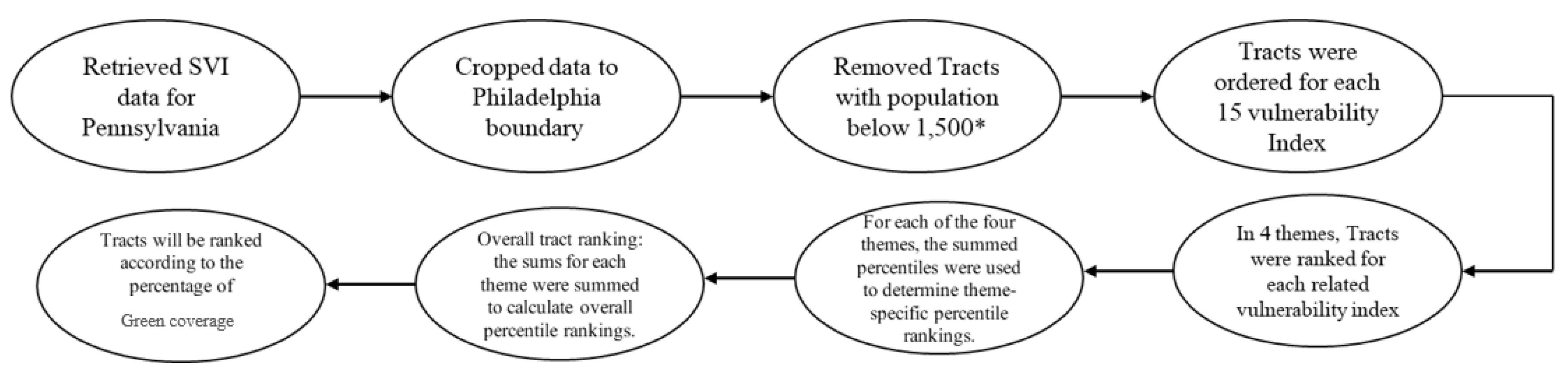
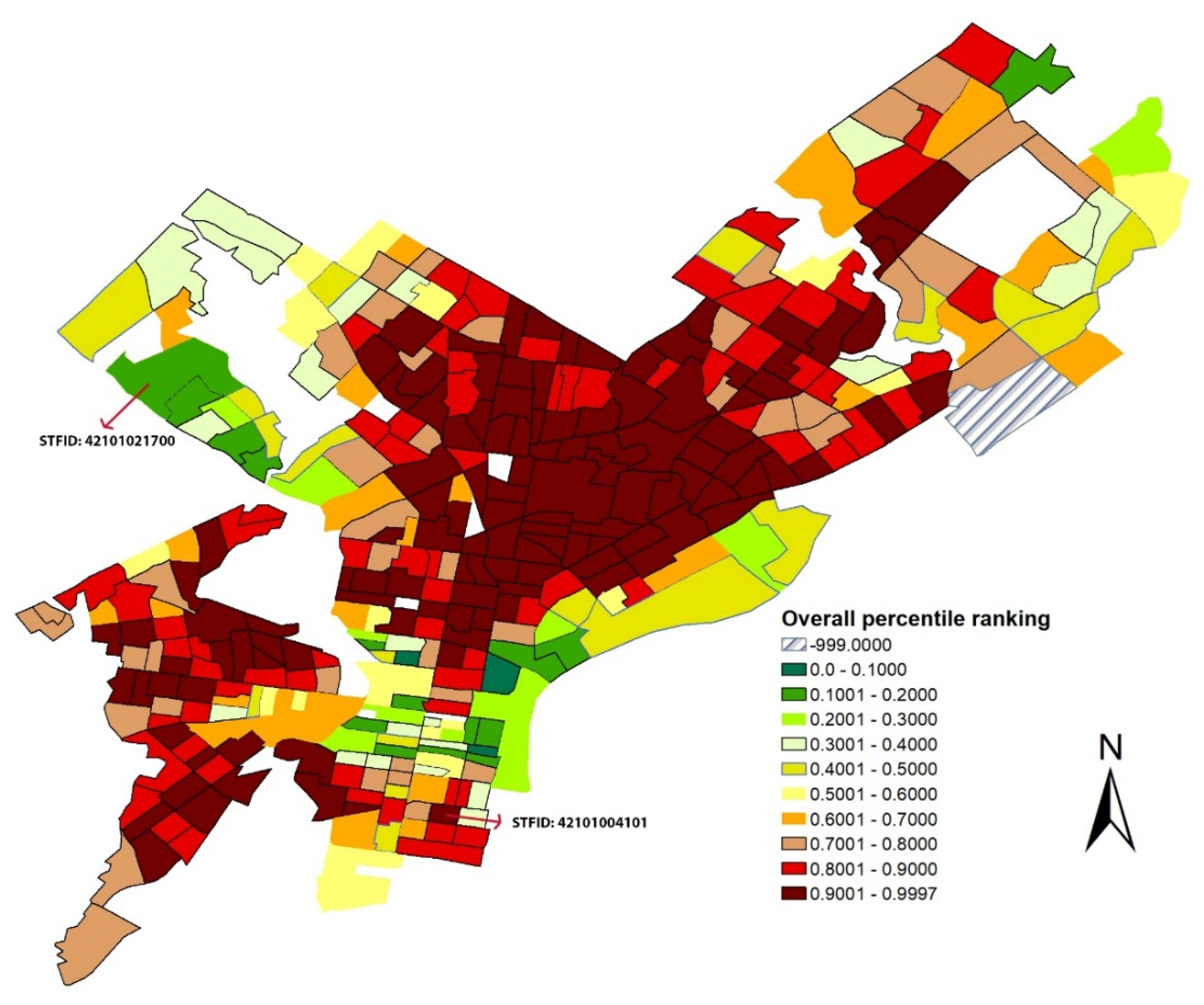
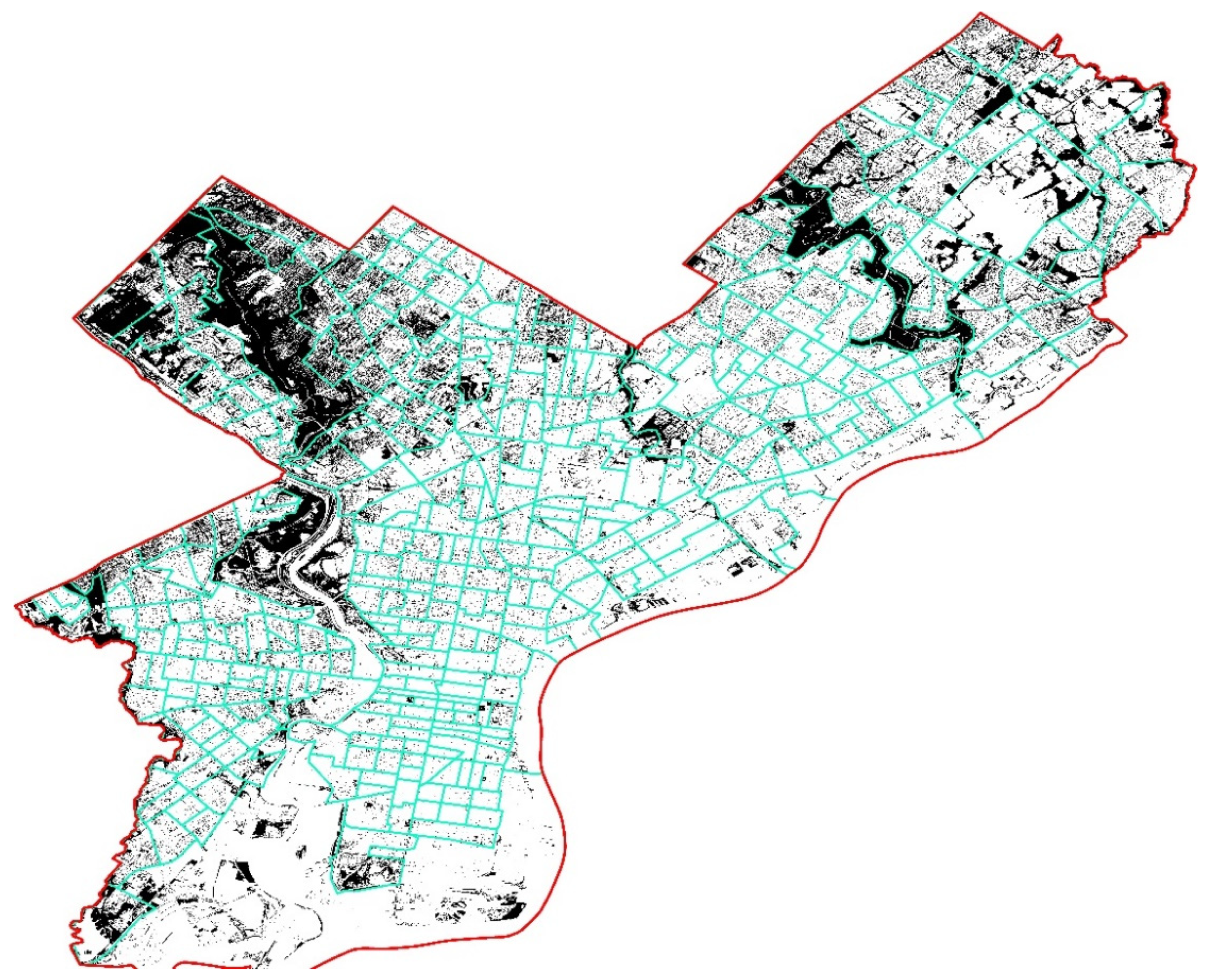
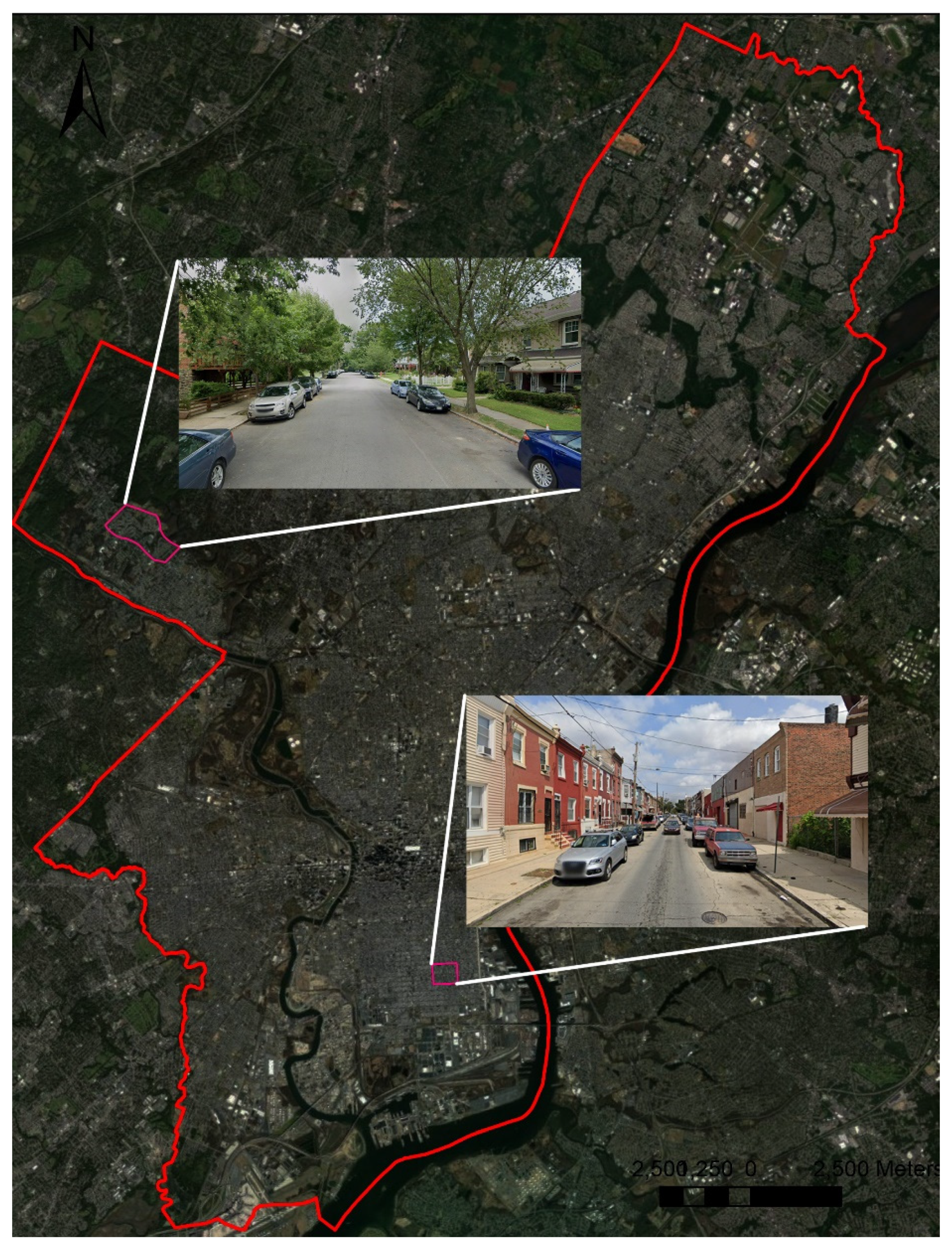
2.1. Step 1: Exploring Social Vulnerability Index to Identify Neighborhoods

Using U.S. Census data, the SVI is gathered by the Agency for Toxic Substances & Disease Registry (ATSDR) at the Centers for Disease Control and Prevention (CDC) to identify the United States communities that will likely need support before, during, and after a public health emergency [43]. Typical census tracts incorporate 1500 to 8000 people, with an optimum size of 4000 people [44], and they are designed to be demographically homogeneous. The CDC/ATSDR SVI ranks U.S. census tracts according to 15 individual variables, i.e., poverty, unemployment, income, education, age (65 or older and 17 or younger), disability, single-parent households, minority, language (speak English less than well), housing unit structure, mobile homes, crowding, lack of vehicle, and group quarter. These 15 variables are further categorized into four related themes including; 1-socioeconomic status, 2-household competition and disability, 3-minority status and language, and 4-housing type and transportation.
The CDC SVI data (2018, the latest version at the time of conducting this research) were used to determine the social vulnerability of every census tract in Philadelphia. Figure 1 shows the tasks to rank the tracts for the four vulnerability themes and the overall vulnerability of the tracts as the last task.
Census tracts in Philadelphia are compared to one another in order to map and analyze relative vulnerability as a consequence of the four aforementioned themes called the overall vulnerability index across the city. Tract rankings are based on percentiles. Percentile ranking values range from 0 (dark green) to 1 (dark red), with higher values indicating greater vulnerability (Figure 2). Tracts for which there is no SVI data available are shown as black and white stripes.
According to the CDC SVI data, census tracts in Philadelphia show significant differences in 15 socioeconomic characteristics, such as poverty, lack of vehicle access, housing type, education, living alone, and disability across the city. Tracts located in northwestern Philadelphia are associated with a low percentile ranking for SVI, 0.1 to 0.2, while tracts in the south, central, and a big part of the north sides show a very high percentile ranking, more than 0.8 indicating greater vulnerability (Figure 2). Moreover, Figure 3 shows a high density of tree canopy in neighborhoods with a low vulnerable population and, on the other hand, a low density of trees in tracts with a higher vulnerability index. Accordingly, the process of selecting two urban blocks in Philadelphia, one with a low level of vulnerability and a high concentration of tree canopy and another with a high level of vulnerability and a low concentration of tree coverage, was achieved by overlaying the SVI and tree canopy coverage from GIS shapefiles.
The outcome of this stage involved the selection of two tracts out of 359 tracts in Philadelphia. One tract was chosen from the tracts with the lowest vulnerability index (STFID: 42101021700, see Figure 2) and high tree coverage, while the other was selected from the tracts with the highest vulnerability index (STFID: 42101004101, see Figure 2) and the lowest tree coverage to proceed with the next step: microclimate modeling. These two tracts and their snapshots are illustrated in Figure 4.

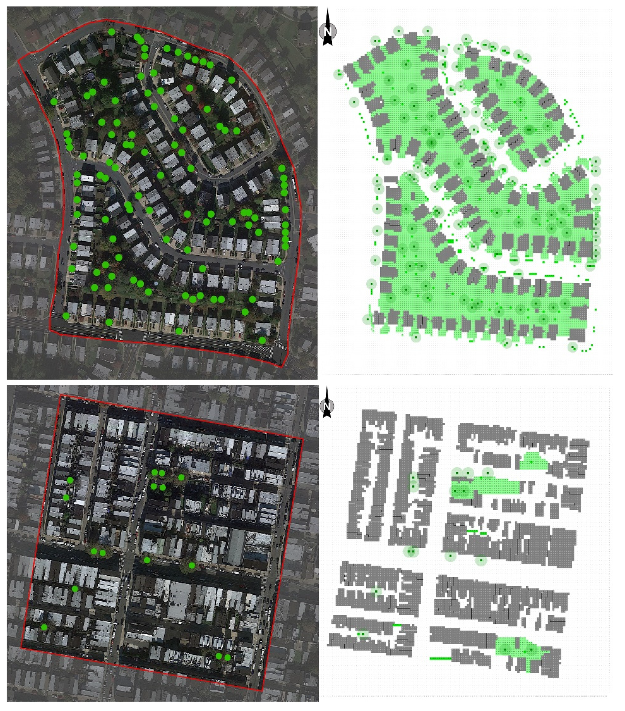
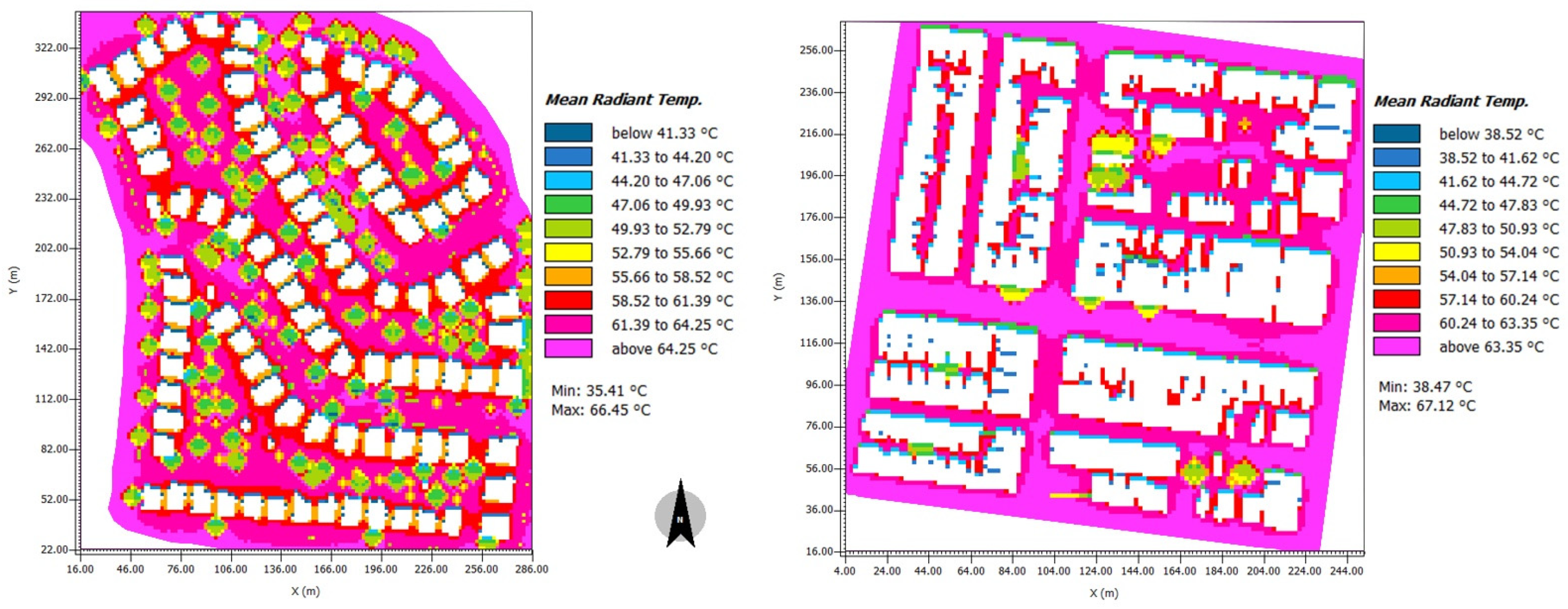
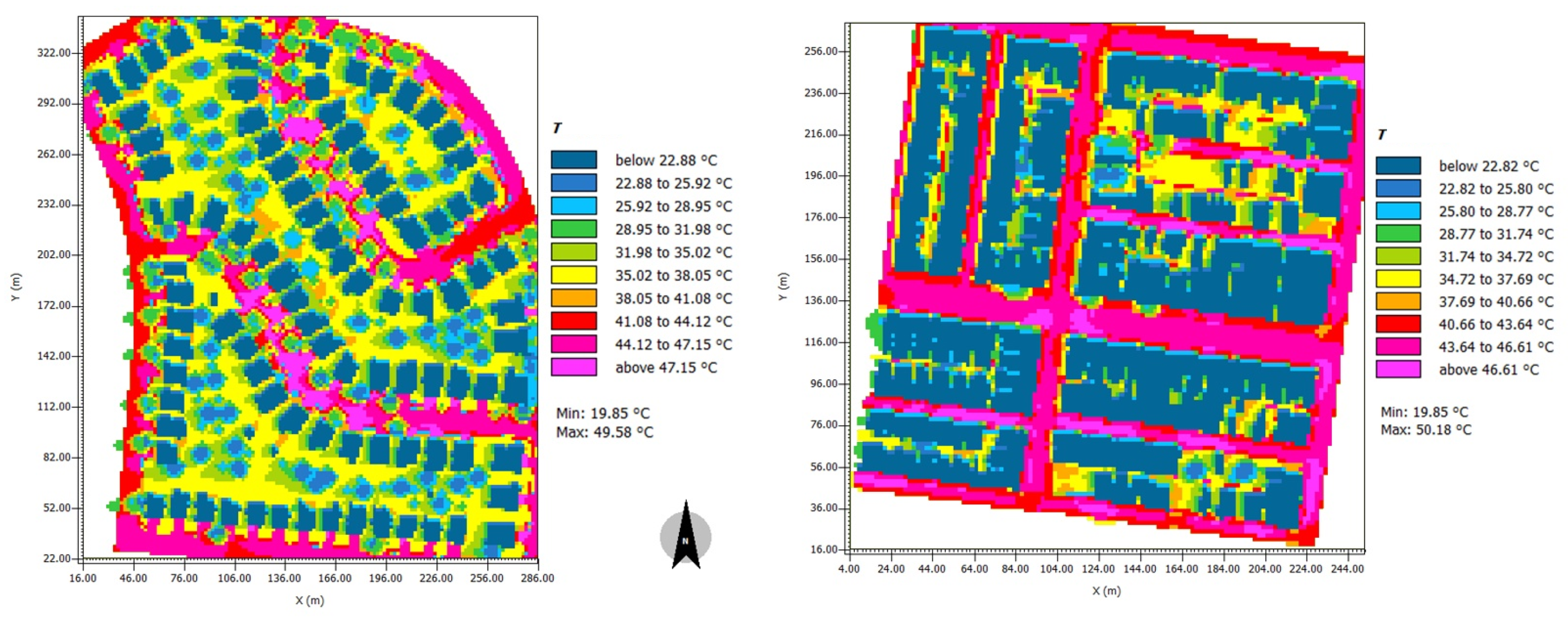
2.2. Step 2: Microclimate and Outdoor Thermal Comfort Simulation

The physical basis and spatial/temporal resolution of urban microclimate models differ greatly. ENVI-met [45], one of the most widely used tools for simulating urban microclimates, can be used to analyze the thermal comfort regime within the street canyon at fine resolutions, down to 0.5 × 0.5 m. The user-friendly tool aims at replicating the primary atmospheric processes that affect the microclimate on a physical basis (i.e., the fundamental laws of fluid dynamics and thermodynamics). BioMet is a plug-in for ENVI-met that calculates human thermal comfort indices from ENVI-met model output files. ENVI-met BIO-met can be used to assess the effects of the presence of vegetation in an urban space, local shading on the person, the position of the person in relation to buildings, and the albedo of paving materials.
ENVI-met BioMet is able to predict outdoor thermal comfort in terms of indices such as a predicted mean vote (PMV), physiological equivalent temperature (PET), universal thermal climate index (UTCI), and standard effective temperature (SET). In this research, the PMV index was adopted to evaluate the outdoor thermal comfort at the street level of the selected tracts in Philadelphia. The PMV is a thermal index developed by Fanger [46] to assess indoor thermal comfort. The PMV calculated by ENVI-met has been adapted for outdoor conditions, including solar radiation and wind speed. To perform a simulation through ENVI-met BioMet, four environmental factors, i.e., air temperature (Ta), mean radiant temperature (MRT), wind speed (UV), and the specific humidity (q), were extracted from the ENVI-met outputs. Moreover, two personal factors, i.e., metabolic rate (ISO 8996) and clothing index (ISO 9920) for four seasons were extracted from the literature [47] and were incorporated into the BIO-met model.
To simulate the PMV index for the selected tracts, two high-resolution 3-D models were created in ENVI-met (Figure 5), with green color representing grass coverage and trees in each model. As a main input to ENVI-met, the geometrical data of the models were obtained from Philadelphia GIS Shapefile, open-source data provided by Pennsylvania Spatial Data Access (PASDA) [48].
In order to construct three-dimensional models of neighborhoods, Grasshopper 3-D and Meerkat, which are based on Rhinoceros software, were utilized. The process of using these tools to create urban 3-D models is explained in detail in [49,50]. The resulting raw 3-D geometries were then imported into Dragonfly, a plug-in created [51] for use in Grasshopper, which enables the creation of 3-D models using Envi-met (INX). To incorporate specific urban characteristics, such as construction materials, land cover, albedo, and anthropogenic heat generated by human activities, the two areas under investigation were classified based on the local climate zone (LCZ) system. The LCZs categorize landscapes based on a typical range of values for surface cover, urban structure, fabrics (radiative and thermal properties of construction materials), and anthropogenic heat flux [52]. The LCZ classification scheme consists of 10 built and 7 land cover types, and each of the 17 basic types is associated with typical value ranges for a set of key urban parameters. The definition and physical properties of all LCZs are provided in 17 illustrative datasheets. Accordingly, the tract with STFID of 42101021700 (top images in Figure 4, simply Block 1, hereafter) was classified as LCZ6: Open low-rise, where buildings are detached and small size with 1–3 stories tall. On the other hand, the tract with the STFID of 42101004101 (bottom images in Figure 4, simply Block 2, hereafter) was classified as LCZ 3: Compact low-rise in which buildings are attached or closely spaced with 1–3 stories tall. Land cover in LCZ 3 is mostly paved or hard-packed; LCZ6 is mostly covered by scattered trees and abundant plants (Figure 6). In order to balance the need for accurate simulation results with the computational time required, the 3-D models were constructed for only a portion of the selected tracts. Specifically, the models were created to cover an area with a minimum diameter of 400 m (or a radius of 200 m), which is the minimum size specified in the LCZ description.
Table 1 summarizes the details of each model for geometrical data and urban configuration. Although the buildings in the two models have almost the same height (6 to 7 m), other properties such as greenery area, site coverage by built elements, and pavement coverage are substantially different between the two models. Additionally, the canyon aspect ratio, height-to-width (H/W), for streets located within Block 1 is consistently 0.25; this ratio varies for streets in different directions within Block 2. Specifically, the H/W ratio in Block 2 ranges from 0.32 for primary East-West streets to 0.8 for secondary streets in the North-South and East-West directions.
In total, 180 h of medium forcing and parallel microclimate simulations were conducted for the two models. Each model was subject to six different weather scenarios, with four scenarios for each of the four seasons (winter, spring, summer, and fall), as well as two scenarios for extreme hot and cold days. The simulations were conducted separately for each scenario, using weather data obtained from the National Oceanic and Atmospheric Administration (NOAA) for the year 2021, which included hourly measurements of air temperature, relative humidity, wind speed, and wind direction and are listed in Table 2. To represent each season, average data for a month within each season (February, May, July, and October) were selected. The literature suggests beginning the simulation process during the early hours of the morning, specifically after sunrise, as this time is characterized by stable atmospheric conditions and minimal impact from the warming effects of the sun on the urban environment [33,53]. Therefore, the simulation for each case was started at 06:00 a.m. and lasted for 24 h to accurately reproduce the characteristics of the selected day.

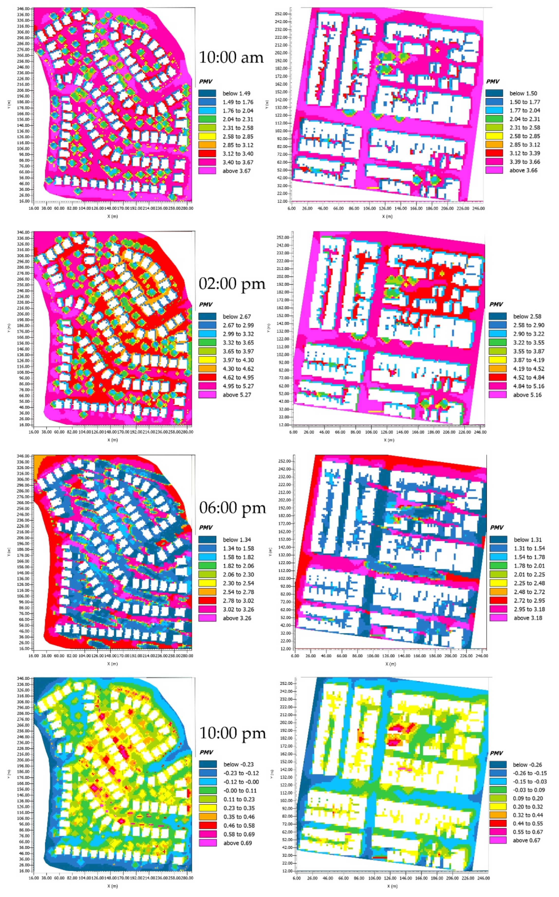
3. Results and Discussion

To determine the climate variables and outdoor thermal comfort in various seasons, fine-level (2 m × 2 m) microclimate and the PMV index were simulated using the ENVI-met and BIO-met models, respectively. As it has been mentioned, 24 h microclimate simulation for six scenarios (winter, spring, summer, fall, extreme hot, and extreme cold) was run for the two models. It means, for example, the PMV inside one model was simulated 144 times to cover 24 h of the six scenarios. After conducting simulations for all six scenarios, the ENVI-met Leonardo tool was employed to visualize the results.
Figure 7 depicts the mean radiant temperature (MRT) simulated at a height of 1.5 m above the ground level at noon for the two blocks. MRT is considered the most important meteorological factor for evaluating outdoor thermal sensation under sunny conditions, regardless of the comfort index used [54]. The MRT range for both models is almost identical, with values exceeding 60 °C for streets that are fully exposed to solar radiation and constructed with asphalt. However, the effects of shading and evapotranspiration from trees result in a range of MRTs between 47 °C and 51 °C for areas below or close to trees (yellow to green areas), leading to an average MRT of 54.5 °C at street level in Block 1, while a very low number of trees in Block 2 led to an average simulated MRT of 61.5 °C. It should be noted that the average values are calculated for the entire street surfaces, including areas under trees and other surfaces made of asphalt and concrete pavement. The influence of grass coverage on MRTs was negligible, with grassy areas exhibiting MRTs that were at most 2 °C lower than other surfaces in the two blocks. Additionally, the simulations revealed a minimum MRT of 35.41 °C and 38.47 °C and a maximum of 66.45 °C and 67.12 °C for Block 1 and Block 2, respectively.
Figure 8 provides a visual comparison of surface temperatures for the summer case at noon. It should be noted that the dark blue areas represent the footprint of buildings and are excluded from the surface temperature analysis. These areas are not reflective of the surface material or vegetation cover and, therefore, would not provide accurate information on surface temperatures. However, the maps show significant differences in surface temperatures across various materials, such as asphalt, concrete pavement, and grass areas. Among these materials, the largest temperature difference is observed in asphalt, where the temperature exceeds 47 °C (purple and red areas). In contrast, the lowest temperature of 23 °C (blue areas) is recorded on the surface right below trees. Additionally, the surface temperature of grass areas was simulated at a range between 34.5 °C to 38 °C (yellow areas). Accordingly, Block 1, with almost 48% covered by grass, benefits from shading and cooling effects that mitigate heat buildup on surfaces compared to Block 2, with only 0.02% grass coverage but 40% covered by impervious surfaces such as asphalt and concrete pavement.
The output files from ENVI-met, along with two personal factors, i.e., metabolism rate and clothing index for each season were incorporated into ENVI-met BioMet to simulate the PMV indices. The PMV model is based on heat balance principles and connects six crucial elements of thermal comfort to the average human response on a specified scale. Normally, the PMV scale is defined on a seven-point thermal sensation scale ranging from cold (−3) to neutral or comfort (0) to hot (+3).
In Figure 9, the output of the ENVI-met model is shown as PMV index maps for the summer scenario at four different hours of the day: 10:00 am, 02:00 pm, 06:00 pm, and 10:00 pm. Maps in Figure 9 serve as examples to demonstrate the variations of comfort index across the models’ area at different hours, and findings are explained in the following sections.
  • PMV values at 10:00 am, summer
According to the results of the simulations, the PMV values at street level and grass areas that were fully exposed to the sun were above 3, which indicates a hot environment and is represented by red to pink colors in the output maps of both models. For areas near or directly below trees, PMV values were recorded in a range from slightly warm (PMV = 1.5) to warm (PMV = 2.5), as indicated by the blue to yellow colors in the maps. For areas located 2 to 4 m to the north or northwest of the building geometries, the PMV values were recorded at the lowest value, below 2, which represents a slightly warm environment. However, no spot was found within the two models that had a PMV value lower than 1, which is the comfort range.
  • PMV values at 02:00 pm, summer
Based on the ENVI-met output maps at 2:00 pm, it can be observed that the entire areas of the two blocks showed PMV values higher than 2.5, which indicates a warm environment. These PMV values were recorded in a few spots located under trees or in areas 2 to 4 m to the north or northeast of the buildings, as shown by light to dark blue colors in the maps. However, spots located on grass areas, asphalt, and concrete pavement all showed PMV values higher than 4, which represents a very hot environment. This indicates that the shading effects of the trees were able to provide some relief from the heat, but other areas that were fully exposed to solar radiation experienced extremely hot conditions.
  • PMV values at 06:00 pm, summer
During the simulation at 6:00 pm, there were still no spots found in both Block 1 or Block 2 with PMV values within the comfort range. However, spots that were affected by trees or located at a distance of 2 to 10 m on the east side of the buildings showed PMV values between 1 and 2, indicating a slightly warm environment. Based on the results, the shading effect of trees and buildings had a significant impact on reducing the PMV index compared to spots on the street level, which had PMV values higher than 3, indicating a hot environment.
Upon comparing the maps of the two blocks, it was observed that Block 1, which had more trees, had more areas with blue color (light to dark), indicating a lower average of PMV values compared to Block 2.
  • PMV values at 10:00 pm, summer
The simulation results for 10:00 pm indicate that nearly all spots within Blocks 1 and 2 have PMV values ranging between −0.5 to +0.5, which is within the comfort range. This suggests that trees and buildings have no significant impact on the PMV values after sunset. It should be noted that this result is observed regardless of the location of the spot within the two blocks, whether it is influenced by trees or buildings. Overall, the PMV values at 10:00 pm suggest that the thermal comfort conditions have improved significantly within the urban environment of the two blocks.
The findings from the summer scenario and the other five weather scenarios demonstrate a strong correlation between tree and grass coverage and outdoor air temperature, mean radiant temperature, and surface temperature during hot seasons and extreme heat events. Areas with a higher concentration of tree canopies experienced a maximum reduction of 1.5 °C in outdoor air temperatures and up to 31 °C in mean radiant temperatures during the daytime of summer and extremely hot conditions. The effects of greenery were more significant in Block 1 (associated with a low SVI), where nearly 50% of the site was covered by trees and grass, compared to only 0.02% of Block 2 (associated with a high SVI). However, the benefits of tree and grass coverage were limited to their immediate surroundings, with areas without green coverage exhibiting significantly higher mean radiant temperatures.
Furthermore, the results showed a strong relationship between PMV and MRT, with a Pearson correlation analysis indicating a significant correlation of 0.987. A significant correlation of 0.859 was also found between air temperature and PMV. The study also found that a higher tree canopy cover in Block 1 was associated with lower outdoor heat exposure in that area, while more impervious surfaces such as streets and pavements in Block 2 were linked to higher heat exposure in that area.
To obtain a more accurate representation of the simulated climate variables and comfort index in the two models, the study included nine specific points for closer investigation, as shown in Figure 10. These points were strategically placed in primary and secondary streets, on asphalt surfaces, sidewalks, and under trees, with the street direction either running from North to South or East to West. The nine specific points were named as follows:
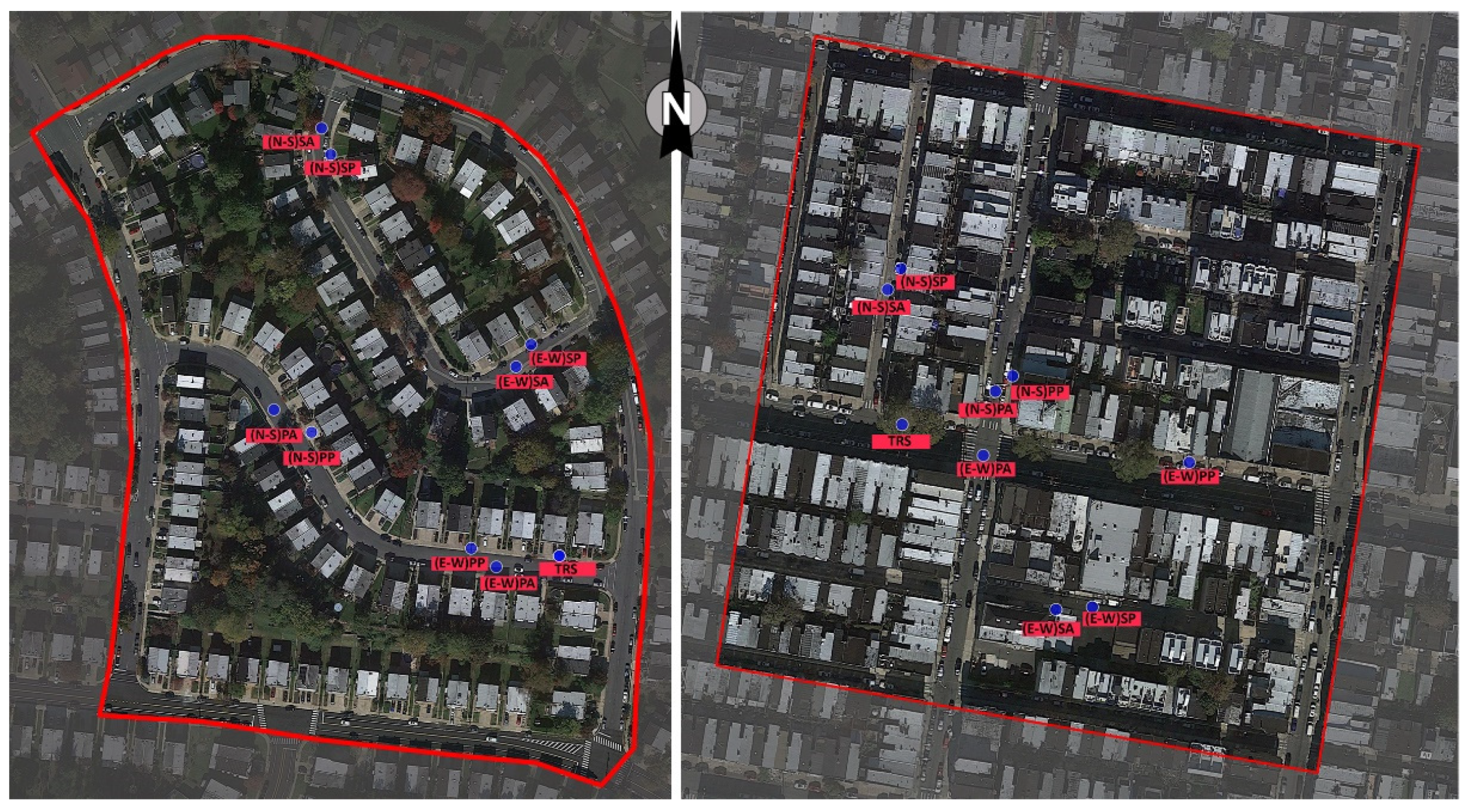
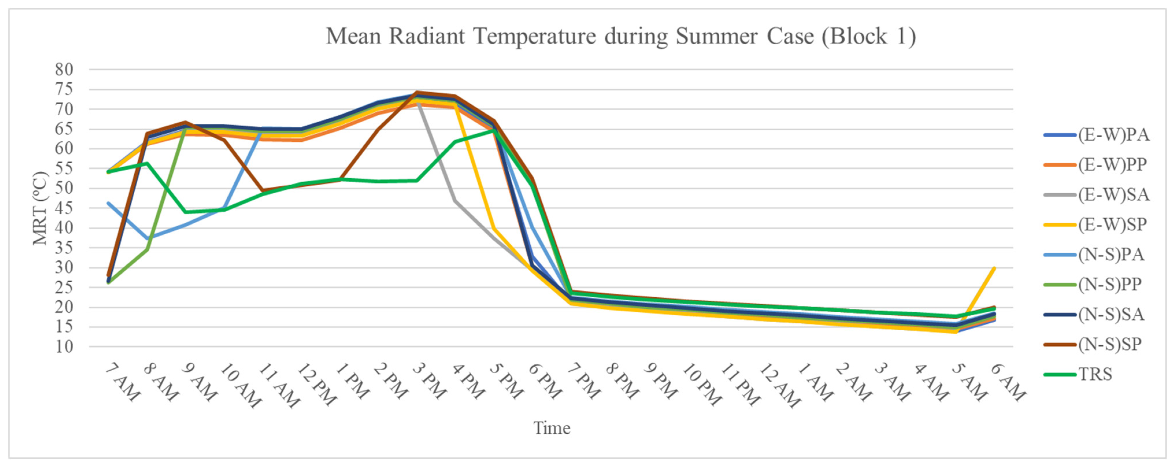
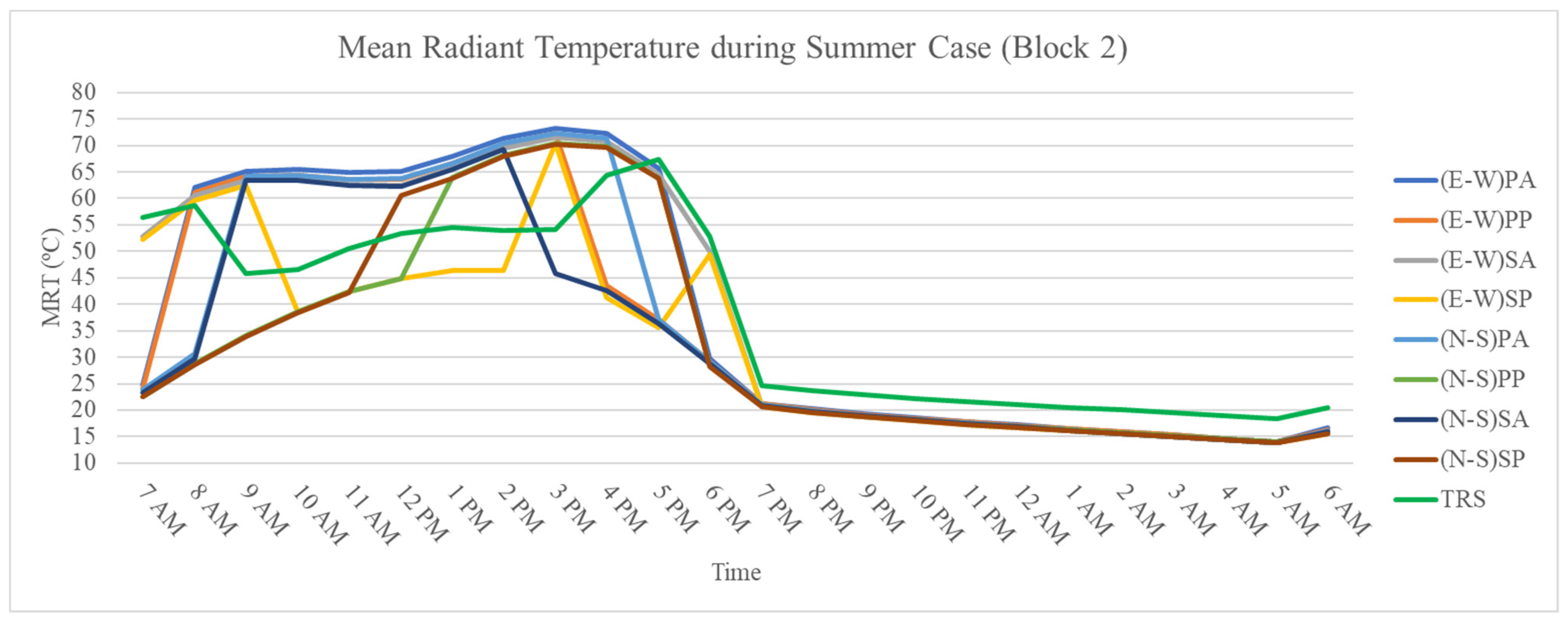
  • North to South primary street, on asphalt (N-S)PA
  • East to West primary street, on asphalt (E-W)PA
  • North to South secondary street, on asphalt (N-S)SA
  • East to West secondary street, on asphalt (E-W)SA
  • North to South primary street, on pavement (N-S)PP
  • East to West primary street, on pavement (E-W)PP
  • North to South secondary street, on pavement (N-S)SP
  • East to West secondary street, on pavement (E-W)SP
  • Under Tress (TRS)
By selecting points in different locations, the study was able to gather data on the varying effects of different surface types and orientations, which allowed for a more nuanced analysis of the simulated climate variables and their impact on human comfort. Figure 11 and Figure 12 illustrate hourly MRTs simulated at each point inside Block 1 and 2 during the summer case, respectively. The simulation was programmed to take measurements every hour, starting at 6:00 am and ending at 6:00 am, 24 h overall.
The points located under trees showed lower mean radiant temperatures (MRTs) throughout the daytime compared to other points. For further investigation of the impact of other factors on MRT and PMV, the other eight points were selected at places without tree and greenery effects. The urban morphology parameters, including Sky View Factor (SVF), Albedo, and H/W ratio, were recorded at each point and analyzed for their effect on MRT and PMV (Table 3). These parameters describe the physical characteristics of urban environments, and they can affect various aspects of the urban environment, including microclimate and human comfort.
In Block 1, six points showed the approximately same amount of MRT during the daytime, while the other three points, including (N-S)PA, (N-S)SP, and TRS, showed lower MRT values at certain times between 7:00 am and 7:00 pm. For instance, the point located on the primary asphalt in the North-South direction, (N-S)PA, showed a value of 45 °C at 7:00 am, 37 °C at 8:00 am, 40 °C at 9:00 am, and 45 °C at 10:00 am. For the rest of the day, MRT recorded at this point was similar to that of other points, which was above 65 °C. The MRT at the point located on the pavement surface of the secondary street in the North-South direction, (N-S)SP, fluctuated between 65 °C at 9:00 am and 50 °C at noon, returning to the same amount as other points after 3:00 pm. The point located under a tree (TRS) had lower MRT throughout the daytime, with a maximum value of 20 °C at 9:00 am compared to the other points.
In Block 2, MRT recorded at two points was lower than other points, including the TRS point, during the morning. These two points were both in the North-South direction and located on both asphalt and pavement surfaces in a secondary street. These two points were well-shaded by the surrounding building, especially buildings on the right side that blocked east sun radiation.
Although the H/W ratio was constant (0.25 for all the points) inside Block 1, SVF and albedo showed a strong effect on MRTs and PMV. A Pearson correlation of 0.61 was found between SVF and MRTs inside Block 1, while it was found up to 0.75 inside Block 2. It means that points with higher SVF have more exposure to heat, resulting in higher MRTs and PMV. Conversely, the urban morphology parameter of albedo displayed a negative correlation of −0.60 with MRTs inside Block 1 and −0.55 inside Block 2, indicating a significant yet inverse relationship. Thus, it can be inferred that higher albedo values correspond to lower MRTs. In Model 2, where different streets had varying H/W ratios, the coefficient with MRTs was −0.39, suggesting that this parameter also has a notable impact on MRT values.

4. Conclusions

This research presented a method that integrates a climate classification system with a 3-D microclimate model to investigate the correlation between outdoor urban climate and the socioeconomic status of urban blocks, using two urban blocks in Philadelphia, Pennsylvania, USA, as the study case. The study involved creating and simulating microclimate models in two urban blocks, which were extracted from two census tracts with varying vulnerability indices. The results demonstrated that urban morphological factors such as vegetated areas, sky view factor (SVF), albedo, and height-to-width (H/W) ratio have an influence on air temperature, mean radiant temperature (MRT), and predicted mean vote (PMV).
The study revealed that trees have a significant cooling effect on outdoor air temperature, MRT, and PMV index during the summer day scenario. These findings are consistent with previous research [55,56,57] that highlighted the beneficial impacts of urban vegetation and roadside trees on the microclimate by reducing surface temperature and MRT, increasing evapotranspiration, providing shading, and reducing PMV. However, the study also found that the benefits of trees are limited to their immediate surroundings, with areas lacking green coverage exhibiting significantly higher MRTs. Consistent with the finding from [56], this study shows the effect of trees on air temperature decreases with increasing distance from the tree canopy.
The study also revealed that the impact of the H/W ratio and surface albedo on outdoor thermal comfort is significant, with higher H/W ratios and albedo leading to lower MRT and greater comfort levels, which is consistent with findings from [53,58,59]. Furthermore, the results presented in this research align with those of a study conducted by [60], which also indicated that factors related to urban morphology, such as building density and orientation, play a notable role in influencing microclimate parameters and thermal comfort.
In conclusion, it is recommended that the utilization of taller and denser buildings with higher albedo pavement surfaces should be considered to enhance thermal comfort conditions, particularly in urban blocks with limited vegetation coverage. The proposed workflow provides evidence to support incorporating urban climate knowledge into the planning and design of healthful and resilient urban environments. Overall, the study highlights the importance of considering urban morphology and vegetation coverage in the design of sustainable and livable urban environments.
This research could be extended in four directions. First, the research involved a 24-h simulation cycle, while it is recommended for future studies to extend the timeframe to 48-h or 72-h cycles to obtain a more comprehensive understanding. Second, the ENVI-met models were supplemented with generic data from the LCZ datasheet for building typology and properties. However, to improve accuracy, genuine information on building materials, A/C types, green roofs and walls, and blue (water) surfaces, if available within the studied blocks, can be added to the models. Third, the research solely concentrated on outdoor weather variables and comfort levels. However, researchers in this era are interested in indoor comfort, which can be investigated in future works. Last, the research concentrated on Philadelphia, PA, from the U.S. Northeast region. However, to gain a better understanding of the effects of urban properties on outdoor climate variables and thermal comfort inside urban blocks with varying social vulnerability indexes, this research should be expanded to incorporate more cities from other climate zones, including hot and dry or extremely cold.

Author Contributions

Conceptualization, F.H., U.P., L.D.I. and G.C.; methodology, F.H. and U.P. and G.C.; software, F.H.; writing—original draft preparation, F.H.; review and editing, U.P., L.D.I. and G.C. All authors have read and agreed to the published version of the manuscript.

Funding

This research was supported in part by the National Science Foundation (Award #2207436), the USDA National Institute of Food and Agriculture and Multistate Research Project (#PEN04623; Accession #1013257), the Eunice Kennedy Shriver National Institute of Child Health and Human Development (Award #P2C HD041025), and the 2021 Institute of Energy and the Environment (IEE) seed grant program at the Pennsylvania State University.

Data Availability Statement

The data presented in this study are available on request from the corresponding author.

Acknowledgments

The authors are grateful for the support from the Hamer Center for Community Design, a research arm of Stuckeman School, and the Department of Architecture at the Pennsylvania State University. Additionally, the authors acknowledge the contributions of Yosef Bodovski, a GIS research analyst at Penn State’s Computational and Spatial Analysis (CSA) Core, for his aid with the GIS maps.

Conflicts of Interest

The authors declare no conflict of interest.

References

  1. Masson-Delmotte, T.W.; Zhai, P.; Pörtner, H.-O.; Roberts, D.; Skea, J.; Shukla, P.R.; Pirani, A.; Moufouma-Okia, W.; Péan, C.; Pidcock, R.; et al. Global Warming of 1.5 °C. An IPCC Special Report on the Impacts of Global Warming of 1.5 °C above Pre-industrial Levels and Related Global Greenhouse Gas Emission Pathways, in the Context of Strengthening the Global Response to the Threat of Climate Change. 2018. Available online: https://www.ipcc.ch/sr15/ (accessed on 17 February 2022).
  2. P. D. United Nations, Department of Economic & Social Affairs. World Urbanization Prospects: The 2018 Revision; United Nations: New York, NY, USA, 2019; Available online: https://population.un.org/wup/publications/Files/WUP2018-Report.pdf (accessed on 13 March 2022).
  3. Taha, H. Urban climates and heat islands: Albedo, evapotranspiration, and anthropogenic heat. Energy Build. 1997, 25, 99–103. [Google Scholar] [CrossRef] [Green Version]
  4. Unger, J. Connection between urban heat island and sky view factor approximated by a software tool on a 3D urban database. Int. J. Environ. Pollut. 2009, 36, 59. [Google Scholar] [CrossRef] [Green Version]
  5. Landsberg, H.E. Urban energy fluxes. In The Urban Climate; University of Maryland: College Park, MD, USA, 1981; pp. 53–82. [Google Scholar]
  6. Oke, T.R. The energetic basis of the urban heat island. Q. J. R. Meteorol. Soc. 1982, 108, 1–24. [Google Scholar] [CrossRef]
  7. Taha, H. Characterization of Urban Heat and Exacerbation: Development of a Heat Island Index for California. Climate 2017, 5, 59. [Google Scholar] [CrossRef] [Green Version]
  8. Santamouris, M. Science of the Total Environment Analyzing the heat island magnitude and characteristics in one hundred Asian and Australian cities and regions. Sci. Total Environ. 2015, 512–513, 582–598. [Google Scholar] [CrossRef]
  9. Peng, S.; Piao, S.; Ciais, P.; Friedlingstein, P.; Ottle, C.; Bréon, F.-M.; Nan, H.; Zhou, L.; Myneni, R.B. Surface Urban Heat Island Across 419 Global Big Cities. Environ. Sci. Technol. 2011, 46, 696–703. [Google Scholar] [CrossRef] [PubMed]
  10. Estoque, R.C.; Murayama, Y.; Myint, S.W. Science of the Total Environment Effects of landscape composition and pattern on land surface temperature: An urban heat island study in the megacities of Southeast Asia. Sci. Total. Environ. 2017, 577, 349–359. [Google Scholar] [CrossRef] [PubMed]
  11. Ho, H.C.; Knudby, A.; Chi, G.; Aminipouri, M.; Lai, D.Y.-F. Spatiotemporal analysis of regional socio-economic vulnerability change associated with heat risks in Canada. Appl. Geogr. 2018, 95, 61–70. [Google Scholar] [CrossRef] [PubMed]
  12. Khatana, S.A.M.; Werner, R.M.; Groeneveld, P.W. Association of Extreme Heat with All-Cause Mortality in the Contiguous US, 2008–2017. JAMA Netw. Open 2022, 5, e2212957. [Google Scholar] [CrossRef]
  13. Centers for Disease Control and Prevention. National Environmental Public Health Tracking Network. 2023. Available online: www.cdc.gov/ephtracking (accessed on 10 May 2022).
  14. Anderson, G.B.; Bell, M.L. Heat Waves in the United States: Mortality Risk during Heat Waves and Effect Modification by Heat Wave Characteristics in 43 U.S. Communities. Environ. Health Perspect. 2011, 119, 210–218. [Google Scholar] [CrossRef] [Green Version]
  15. Heaton, M.J.; Sain, S.R.; Greasby, T.A.; Uejio, C.K.; Hayden, M.H.; Monaghan, A.J.; Boehnert, J.; Sampson, K.; Banerjee, D.; Nepal, V.; et al. Characterizing urban vulnerability to heat stress using a spatially varying coefficient model. Spat. Spatio-Temporal Epidemiol. 2014, 8, 23–33. [Google Scholar] [CrossRef] [PubMed]
  16. Madrigano, J.; Ito, K.; Johnson, S.; Kinney, P.L.; Matte, T. A Case-Only Study of Vulnerability to Heat Wave—Related Mortality. Environ. Health Perspect. 2015, 123, 672–678. [Google Scholar] [CrossRef] [PubMed]
  17. Hsu, A.; Manya, D. Intensity across Major US Cities. Nat. Commun. 2021, 12, 2721. [Google Scholar] [CrossRef] [PubMed]
  18. Yang, W.; Wong, N.H.; Jusuf, S.K. Thermal comfort in outdoor urban spaces in Singapore. Build. Environ. 2013, 59, 426–435. [Google Scholar] [CrossRef]
  19. Aljawabra, F.; Nikolopoulou, M. Thermal comfort in urban spaces: A cross-cultural study in the hot arid climate. Int. J. Biometeorol. 2018, 62, 1901–1909. [Google Scholar] [CrossRef]
  20. Salata, F.; Golasi, I.; Vollaro, R.D.L.; Vollaro, A.D.L. Outdoor thermal comfort in the Mediterranean area. A transversal study in Rome, Italy. Build. Environ. 2016, 96, 46–61. [Google Scholar] [CrossRef]
  21. Huang, J.; Zhou, C.; Zhuo, Y.; Xu, L.; Jiang, Y. Outdoor thermal environments and activities in open space: An experiment study in humid subtropical climates. Build. Environ. 2016, 103, 238–249. [Google Scholar] [CrossRef] [Green Version]
  22. Xu, M.; Hong, B.; Mi, J.; Yan, S. Outdoor thermal comfort in an urban park during winter in cold regions of China. Sustain. Cities Soc. 2018, 43, 208–220. [Google Scholar] [CrossRef]
  23. Hirashima, S.Q.D.S.; de Assis, E.S.; Nikolopoulou, M. Daytime thermal comfort in urban spaces: A field study in Brazil. Build. Environ. 2016, 107, 245–253. [Google Scholar] [CrossRef] [Green Version]
  24. Middel, A.; Selover, N.; Hagen, B.; Chhetri, N. Impact of shade on outdoor thermal comfort—A seasonal field study in Tempe, Arizona. Int. J. Biometeorol. 2016, 60, 1849–1861. [Google Scholar] [CrossRef] [Green Version]
  25. Chi, G.Q.; Ho, H.C. Population stress: A spatiotemporal analysis of population change and land development at the county level in the contiguous United States, 2001–2011. Land Use Policy 2018, 70, 128–137. [Google Scholar] [CrossRef]
  26. Chi, J.; Zhu, G. Spatial Regression Models for the Social Sciences; SAGE Publications: Thousand Oaks, CA, USA, 2019. [Google Scholar]
  27. Toparlar, Y.; Blocken, B.; Maiheu, B.; van Heijst, G. A review on the CFD analysis of urban microclimate. Renew. Sustain. Energy Rev. 2017, 80, 1613–1640. [Google Scholar] [CrossRef]
  28. Crank, P.J.; Sailor, D.J.; Ban-Weiss, G.; Taleghani, M. Evaluating the ENVI-met microscale model for suitability in analysis of targeted urban heat mitigation strategies. Urban Clim. 2018, 26, 188–197. [Google Scholar] [CrossRef]
  29. Ozkeresteci, I.; Crewe, K.; Brazel, A.J.; Bruse, M. Use and evaluation of the ENVI-met model for environmental design and planning. An Experiment on Lienar Parks. In Proceedings of the 21st International Cartographic Conference (ICC), Durban, South Africa, 10–16 August 2003; pp. 10–16. [Google Scholar]
  30. Rodríguez Algeciras, J.A.; Gómez Consuegra, L.; Matzarakis, A. Spatial-temporal study on the effects of urban street configurations on human thermal comfort in the world heritage city of Camagüey-Cuba. Build. Environ. 2016, 101, 85–101. [Google Scholar] [CrossRef]
  31. Sinsel, T. Advancements and Applications of the Microclimate Model ENVI-Met; Johannes Gutenberg-Universitat Mainz: Mainz, Germany, 2022. [Google Scholar] [CrossRef]
  32. Ayyad, Y.N.; Sharples, S. Envi-MET validation and sensitivity analysis using field measurements in a hot arid climate. IOP Conf. Series Earth Environ. Sci. 2019, 329, 012040. [Google Scholar] [CrossRef] [Green Version]
  33. Acero, J.A.; Arrizabalaga, J. Evaluating the performance of ENVI-met model in diurnal cycles for different meteorological conditions. Theor. Appl. Clim. 2018, 131, 455–469. [Google Scholar] [CrossRef]
  34. Acero, J.A.; Herranz-Pascual, K. A comparison of thermal comfort conditions in four urban spaces by means of measurements and modelling techniques. Build. Environ. 2015, 93, 245–257. [Google Scholar] [CrossRef]
  35. Alsaad, H.; Hartmann, M.; Hilbel, R.; Voelker, C. ENVI-met validation data accompanied with simulation data of the impact of facade greening on the urban microclimate. Data Brief 2022, 42, 108200. [Google Scholar] [CrossRef]
  36. Morakinyo, T.E.; Lai, A.; Lau, K.K.-L.; Ng, E. Thermal benefits of vertical greening in a high-density city: Case study of Hong Kong. Urban For. Urban Green. 2019, 37, 42–55. [Google Scholar] [CrossRef]
  37. Forouzandeh, A. Numerical modeling validation for the microclimate thermal condition of semi-closed courtyard spaces between buildings. Sustain. Cities Soc. 2018, 36, 327–345. [Google Scholar] [CrossRef]
  38. Elraouf, R.A.; Elmokadem, A.; Megahed, N.; Eleinen, O.A.; Eltarabily, S. Evaluating urban outdoor thermal comfort: A validation of ENVI-met simulation through field measurement. J. Build. Perform. Simul. 2022, 15, 268–286. [Google Scholar] [CrossRef]
  39. US Census Bureau. 2022. Available online: https://www.census.gov/quickfacts/fact/table/US/PST045222 (accessed on 23 January 2023).
  40. Mayor’s Office of Sustainability and ICF International. Growing Stronger: Toward a Climate-Ready Philadelphia. 2015. Available online: https://www.phila.gov/documents/growing-stronger-toward-a-climate-ready-philadelphia/ (accessed on 1 March 2023).
  41. Schade, R.S. Philadelphia Rowhouse Manual: A Practical Guide for Homeowners; The City of Philadelphia: Philadelphia, PA, USA, 2008. Available online: https://www.phila.gov/media/20190521124726/Philadelphia_Rowhouse_Manual.pdf (accessed on 18 July 2021).
  42. Baechler, P.M.; Michael, C.; Williamson, J.L.; Gilbride, T.L.; Cole, P.C.H.; Marye, G.L. Building America Best Practices Series: Volume 7.1: Guide to Determining Climate Regions by County. 2010. Available online: https://www.osti.gov/biblio/1068658 (accessed on 22 July 2021).
  43. Centers for Disease Control and Prevention/Agency for Toxic Substances and Disease Registry/Geospatial Research, Analysis, and Services Program. 2018. Available online: https://www.atsdr.cdc.gov/placeandhealth/svi/data_documentation_download.html (accessed on 15 June 2021).
  44. U.S. Census Bureau. 2009. Available online: https://www.census.gov/library/publications/2008/compendia/statab/128ed.html (accessed on 21 August 2021).
  45. Bruse, M.; Fleer, H. Simulating surface–plant–air interactions inside urban environments with a three dimensional numerical model. Environ. Model. Softw. 1998, 13, 373–384. [Google Scholar] [CrossRef]
  46. Shaw, E.W. Thermal Comfort: Analysis and applications in environmental engineering, by P. O. Fanger. 244 pp. DANISH TECHNICAL PRESS. Copenhagen, Denmark, 1970. Danish Kr. 76, 50. R. Soc. Health J. 1972, 92, 164. [Google Scholar] [CrossRef] [Green Version]
  47. Havenith, G.; Holmér, I.; Parsons, K. Personal factors in thermal comfort assessment: Clothing properties and metabolic heat production. Energy Build. 2002, 34, 581–591. [Google Scholar] [CrossRef]
  48. Pennsylvania Spatial Data Access PASDA. The Pennsylvania State University. 2016. Available online: http://www.pasda.psu.edu/ (accessed on 15 August 2021).
  49. Hashemi, F.; Marmur, B.; Passe, U.; Thompson, J. Developing a workflow to integrate tree inventory data into urban energy models. In SimAUD 2018 Symposium on Simulation for Architecture and Urban Design; Simulation Series; TU Delft: Delft, The Netherlands, 2018; Volume 50. [Google Scholar]
  50. Hashemi, F.; Iulo, L.D.; Poerschke, U. A novel approach for investigating canopy heat island effects on building energy performance: A case study of Center City of Philadelphia, PA. In Proceedings of the AIA/ACSA Intersections Research Conference: CARBON, Fall Conference Proceedings, Washington, DC, USA, 30 September – 2 October 2020; pp. 197–203. [Google Scholar] [CrossRef]
  51. Roudsari, M.S.; Pak, M.; Smith, A.; Gill, G. Ladybug: A Parametric Environmental Plugin For Grasshopper To Help Designers Create An Environmentally-conscious Design. In Proceedings of the Building Simulation, Chambéry, France, 26–28 August 2013; pp. 3128–3135. [Google Scholar] [CrossRef]
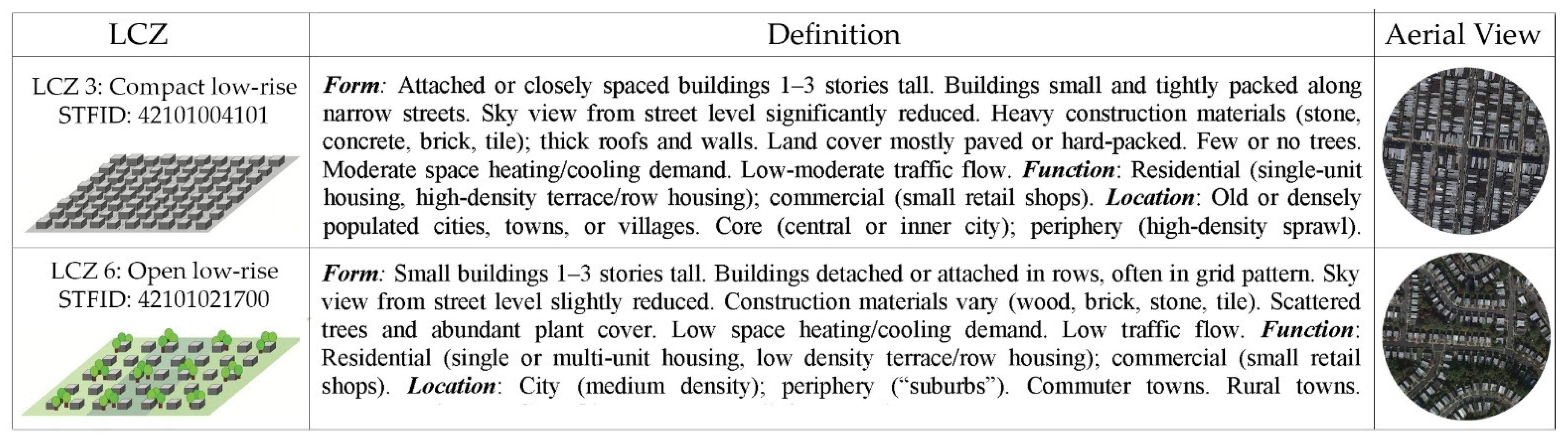
  52. Stewart, I.D.; Oke, T.R. Local Climate Zones for Urban Temperature Studies. Bull. Am. Meteorol. Soc. 2012, 93, 1879–1900. [Google Scholar] [CrossRef]
  53. Ali-Toudert, F.; Mayer, H. Numerical study on the effects of aspect ratio and orientation of an urban street canyon on outdoor thermal comfort in hot and dry climate. Build. Environ. 2006, 41, 94–108. [Google Scholar] [CrossRef]
  54. de Abreu-Harbich, L.V.; Labaki, L.C.; Matzarakis, A. Effect of tree planting design and tree species on human thermal comfort in the tropics. Landsc. Urban Plan. 2015, 138, 99–109. [Google Scholar] [CrossRef]
  55. Gatto, E.; Buccolieri, R.; Aarrevaara, E.; Ippolito, F.; Emmanuel, R.; Perronace, L.; Santiago, J.L. Impact of Urban Vegetation on Outdoor Thermal Comfort: Comparison between a Mediterranean City (Lecce, Italy) and a Northern European City (Lahti, Finland). Forests 2020, 11, 228. [Google Scholar] [CrossRef] [Green Version]
  56. Zaki, S.A.; Toh, H.J.; Yakub, F.; Saudi, A.S.M.; Ardila-Rey, J.A.; Muhammad-Sukki, F. Effects of Roadside Trees and Road Orientation on Thermal Environment in a Tropical City. Sustainability 2020, 12, 1053. [Google Scholar] [CrossRef] [Green Version]
  57. Bernabé, A.; Bernard, J.; Musy, M.; Andrieu, H.; Bocher, E.; Calmet, I.; Kéravec, P.; Rosant, J.-M. Radiative and heat storage properties of the urban fabric derived from analysis of surface forms. Urban Clim. 2015, 12, 205–218. [Google Scholar] [CrossRef] [Green Version]
  58. Elraouf, R.A.; Elmokadem, A.; Megahed, N.; Eleinen, O.A.; Eltarabily, S. The impact of urban geometry on outdoor thermal comfort in a hot-humid climate. Build. Environ. 2022, 225, 109632. [Google Scholar] [CrossRef]
  59. Zhang, Y.; Du, X.; Shi, Y. Effects of street canyon design on pedestrian thermal comfort in the hot-humid area of China. Int. J. Biometeorol. 2017, 61, 1421–1432. [Google Scholar] [CrossRef] [PubMed]
  60. Zaki, S.; Azid, N.; Shahidan, M.; Hassan, M.; Daud, M.; Abu Bakar, N.; Salim, S.A.Z.S.; Yakub, F. Analysis of Urban Morphological Effect on the Microclimate of the Urban Residential Area of Kampung Baru in Kuala Lumpur Using a Geospatial Approach. Sustainability 2020, 12, 7301. [Google Scholar] [CrossRef]
Figure 1. The workflow for ranking Philadelphia’s census tract according to their SVI, Source: Authors.
Buildings 13 01040 g001
Figure 2. Maps show the range of vulnerability in Philadelphia, PA as a consequence of the four themes (overall ranking).
Buildings 13 01040 g002
Figure 3. Tree canopy coverage in Philadelphia, PA.
Buildings 13 01040 g003
Figure 4. Two selected tracts for microclimate simulation; top left with low vulnerability index and bottom right with high vulnerability index, the purple highlights show the exact boundary of each census tract.
Buildings 13 01040 g004
Figure 5. The exact boundary of selected blocks within the census tracts (left images) and ENVI-met models created for each block (right images).
Buildings 13 01040 g005
Figure 6. LCZ description, data adapted from [52], aerial images from Google Earth (Philadelphia, PA).
Buildings 13 01040 g006
Figure 7. Simulated MRT at noon and 1.5 m above the ground level, summer case.
Buildings 13 01040 g007
Figure 8. Simulated Surface temperature at noon, summer case.
Buildings 13 01040 g008
Figure 9. Simulated PMV inside the two models during the summer case for every 4 h starting at 10 am and ending by 10 pm.
Buildings 13 01040 g009
Figure 10. Location of nine points inside the two models.
Buildings 13 01040 g010
Figure 11. MRTs during summer case at nine points inside Block 1.
Buildings 13 01040 g011
Figure 12. MRTs during summer case at nine points inside Block 2.
Buildings 13 01040 g012
Table 1. Model dimensions and site properties for two blocks.
Census BlockModel DimensionsSite Properties
Site AreaNumber of
Buildings
Average Building
Height
Site Coverage
Ratio
Grass Coverage
Ratio
Pavement Coverage
Ratio
Road Coverage
Ratio
H/W Ratio
Block 1152 × 184 × 30
dx = 2 m
dy = 2 m
dz = 2 m
81,182 (m2)1836 m0.210.480.030.280.25
Block 2132 × 137 × 30
dx = 2 m
dy = 2 m
dz = 2 m
53,026 (m2)3027 m0.420.020.180.22Primary E-W: 0.32
Primary N-S: 0.5
Secondary N-S, E-W: 0.8
Table 2. Climatology data for 6 defined cases, source: NOAA.
CasesTmax (°C)Tmin (°C)TAVG (°C)Average Wind Speed (m/s)Wind Direction
Winter Case4.24−1.841.234.35NW
Coldest Day
(2 February 2021)
0−9.99−4.997.07NW
Summer Case3021.625.983.34SW
Hottest Day
(7 July 2021)
35.5224.4229.993.52SW
Fall Case
(24 October 2021)
177.812.473.7SE
Spring Case
(12 May 2021)
20.18.4814.134.11NW
Table 3. SVF, Albedo, and H/W ratio at each point inside two blocks.
BlocksSky View Factor (SVF)Surface AlbedoH/W Ratio
(E-W)PABlock 10.840.20.25
Block 20.780.20.32
(E-W)PPBlock 10.750.350.25
Block 20.680.350.32
(E-W)SABlock 10.840.20.25
Block 20.620.20.8
(E-W)SPBlock 10.810.350.25
Block 20.520.350.8
(N-S)PABlock 10.610.20.25
Block 20.700.20.5
(N-S)PPBlock 10.720.350.25
Block 20.520.350.5
(N-S)SABlock 10.660.20.25
Block 20.610.20.8
(N-S)SPBlock 10.450.350.25
Block 20.510.350.8
Disclaimer/Publisher’s Note: The statements, opinions and data contained in all publications are solely those of the individual author(s) and contributor(s) and not of MDPI and/or the editor(s). MDPI and/or the editor(s) disclaim responsibility for any injury to people or property resulting from any ideas, methods, instructions or products referred to in the content.

