Abstract
One of the most important parameters that indicate the energy performance of a window system is the thermal transmittance (U-value). Many research studies that deal with numerical methods of determining a window’s U-value have been carried out. However, the possible assumptions and simplifications associated with numerical methods and simulation tools could increase the risk of under- or over-estimation of the U-value. For this reason, several experimental methods for investigating the U-value of windows have been developed to be used either alone or as a supplementary method for validation purposes. This review aims to analyze the main experimental methods for assessing the U-value of windows that have been published by national and international standards or as scientific papers. The analysis criteria include the type of the test in terms of boundary conditions (laboratory or in situ), the part of the window that was tested (only the center of glazing or the entire window), and the data analysis method (steady-state or dynamic). The experimental methods include the heat flow meter (HFM) method, guarded hot plate (GHP) method, hot box (HB) method, infrared thermography (IRT) method, and the so-called rapid U-value metering method. This review has been set out to give insights into the procedure, the necessary equipment units, the required length of time, the accuracy, the advantages and disadvantages, new possibilities, and the gaps associated with each method. In the end, it describes a set of challenges that are designed to provide more comprehensive, realistic, and reliable tests.
1. Introduction
As a result of an increase in the global population and the importance of building services and indoor comfort, the building sector’s energy consumption has also increased and is responsible for a considerable share of the total energy used in the world [1,2]. It was reported that in the United States (US), about 41% of primary energy was consumed by the building sector in 2010 [3,4]. In the European Union (EU), this sector accounted for about 40% of the total final energy use and is among the biggest CO2 producers [5]. As China is the largest consumer of world energy, its building sector is expected to consume more than 30% by 2020, according to [4]. Overall, based on the Global Status Report, buildings and constructions are assumed to be responsible for more than 55% of the total global energy consumption [6]. It was reported that the main share of energy consumption in buildings goes to heating and cooling spaces to compensate for the weak performance of building envelopes [7,8,9]. Therefore, the need to improve the thermal performance of building envelopes seems undeniable. To improve the building envelope energy performance, we have to know which parts of the envelope show weaker thermal performance [10,11]. Windows are one of those envelope elements that have received special attention.
Since they provide natural light, natural ventilation, favorable solar gain (in cold regions in the winter), and aesthetic and positive psychological impacts, windows have to be used in buildings [12,13]. However, due to their weak energy performance, windows are one of the most energy-inefficient parts of the building envelope [4]. They account for between 20% and 60% of the energy loss and also excessive solar heat gain in buildings, which depends on factors such as climate and the age, type, and size of buildings [14,15]. It was reported that in the US, windows in commercial buildings were responsible for about 1.5% of the total energy consumption in 2011, which is equivalent to the energy consumption of about 8 million US households [14]. This means that windows have a considerable potential to reduce the total energy consumption of buildings worldwide [16]. Many research studies have been conducted to investigate which features of windows have made their energy inefficient and how they could be improved. Studies have mostly focused on the thermal and optical properties of window systems, followed by their geometries, shapes, and orientation [17,18]. Moghaddam et al. [14] stated that the primary reason for the huge amount of energy loss in buildings would be the high thermal transmittance (U-value) of windows. For traditional single- and double-glazing systems, the U-values are in a range from five to six () and two to three (), respectively [19]. These values are normally much higher than walls, roofs, floors, and doors in such a way that even in the new building codes introduced by European countries, the U-value of windows is allowed to be four–six times the U-value of walls (e.g., in Austria, Belgium, Denmark, Finland, etc.) [20].
The first step in improving a window’s U-value is to evaluate them as accurately as possible [21,22]. However, determining them accurately is not an easy task since both accuracy and simplicity requirements have to be fulfilled [23]. A window system’s U-value can be determined by using laboratory tests and their sub-sequential calculations, theoretical calculations based on national or international standards, and also simulation tools [24]. For homogeneous materials that have one-dimensional steady-state heat flux, the heat transfer analysis is straightforward, while for building elements, such as windows, the inhomogeneity caused by different components and materials constituting the window means that the evaluation of heat transfer would be difficult [3]. In addition, the need to improve the energy performance of windows has resulted in the emergence of new complex window systems, for which the U-value could not be easily calculated via standardized theoretical equations. The mathematical models used in theoretical methods could not help to fully understand the heat transfer behavior inside complex windows [22]. Even if those methods give answers, they should be validated by experimental methods [3,25]. Baldinelli and Bianchi [23] stated that experimental methods could provide researchers with all of the involved heat transfer mechanisms, thereby overcoming the simplifications of numerical procedures. The authors noted that sometimes the simulation results could be under- or over-estimated due to those simplifications. Cuce [26] highlighted the complaints of building occupants about the inadequate thermal performance of commercial glazing products compared to the reported U-values in datasheets, which were mostly derived from theoretical methods or simulation tools. For an argon-filled double-glazed window, the author showed that the experimental U-values (in this case, several environmental chamber tests were conducted) were noticeably higher than those calculated via the theoretical calculation and CFD method. The difference was mostly attributed to the impacts of the thermal bridges and edge effects, which cannot be ignored in the experimental test. Therefore, it was concluded that to determine the U-values of highly insulating and multi-layer fenestration systems, it would be better to adopt experimental methods [23,26]. In addition, there are still complex systems such as supply-air windows, with varying environmental parameters and window parameters for which few numerical solutions have been identified, and those solutions should be complemented and/or validated by reliable experimental methods [27].
This review paper aims to investigate the experimental methods that can determine a window’s U-value following two main steps. First, we examined the main available standardized experimental methods that have been introduced specifically for windows/glazing systems or the standardized methods whose main focus was not on the windows but on adapting and applying window characteristics by other researchers. Second, we looked into the novel experimental methods developed by researchers and whether or not they were based on the main concepts of the available standardized methods. As illustrated in Figure 1, three main criteria were considered for each experimental method: Criterion I which is related to the type of test in terms of boundary conditions (laboratory or in situ); Criterion II, which deals with the part of the window that was analyzed (only the center of the glazing or the entire window, including the edge and frame); and finally, Criterion III, which is related to the data analysis method (steady-state or dynamic).
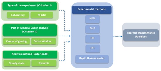
Figure 1.
Schematic of the experimental methods for determining a windows’ U-value with respect to the three main analysis criteria.
The methods reviewed here for the U-value include the heat flow meter (HFM), guarded hot plate (GHP), hot box (HB), infrared thermography (IRT), and the so-called rapid U-value meter. In the end, a set of challenges were identified to provide more comprehensive, realistic, and reliable tests for the future. Figure 2 illustrates the study concept framework.
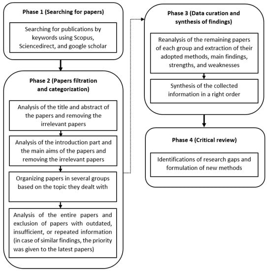
Figure 2.
Illustrates the study concept framework.
2. Experimental Methods for Windows U-Value Determination
Thermal transmittance also called the overall heat transfer coefficient or U-value in (), is generally defined as the steady-state heat flow rate, which is divided by the projected area of a specimen and by the temperature difference between its two sides [7]. As mentioned in ASHRAE Handbook—Fundamentals (ASHRAE 2021) [28], most window systems are made up of transparent multi-pane glazing units and opaque elements, including the frame (and sometimes dividers). Therefore, to obtain the U-value of the entire window, it is necessary to study the heat transfer through the center of the glazing, the edges of the glazing, and the frame part. The first method of the U-value calculation described in ISO 15099:2003 [29], which was subsequently used by the WINDOW simulation tool (developed by Lawrence Berkeley National Laboratory), used the area-weighted U-values of each component of the window according to the following equation:
where U and A represent the U-value () and the projected area () of each part, respectively. The subscripts g, c, e, f, and t indicate the glazing, center, edge, frame, and entire window, respectively.
In the second method of the U-value calculation described in ISO 15099:2003 [29], instead of considering the area of the glazing edge, the term linear thermal transmittance () was used to define the heat transfer through the perimeter of the glass area (). The calculation of the U-value of the entire window is based on the following equation:
Some of the experimental methods that will be explained in the following sub-sections consider the U-value of the entire window, while the other methods consider only the U-value of the central part of the glazing excluding the edges and the frame parts. Therefore, for each method, the parts of the window that are taken into account in the U-value determination are specifically mentioned.
2.1. Heat Flow Meter (HFM) Method
2.1.1. Heat Flow Meter Apparatus
The HFM method is considered one of the most important techniques for thermal conductance and thermal resistance (and subsequently the U-value) determination of building elements [30]. To measure the U-value of the central part of a glazing sample under steady-state conditions, excluding the heat transfer through the frames and linear thermal bridges through the edges, a single- or double-specimen HFM apparatus could be used following standard EN 675:2011 [31] (identical to ISO 10293:1997 [32]). This standard can be applied to multiple glazing with flat and parallel surfaces. The function of an HFM apparatus is based on the temperature difference between the two surfaces of a test specimen, which is created by contacting the hot and cold plate of the HFM apparatus, and the associated heat flux through the sample (perpendicular to the sample) [33]. Figure 3 illustrates the schematic of a single-specimen heat flow meter apparatus. The heating and cooling plates are both similar in size and surface dimensions. A heat flux sensor Is attached to the metering area, as specified in the figure. There is another type of HFM apparatus that supports two specimens. This type of apparatus is made up of a heating plate sandwiched between two specimens and two cooling plates in contact with the samples.
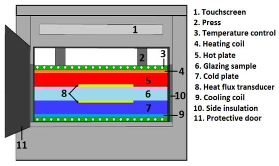
Figure 3.
Schematic of a single-specimen heat flow meter apparatus.
Based on EN 675:2011 [31], the U-value of the glazing under test, in (), can be calculated using the following equation:
where is the surface-to-surface thermal resistance of the glazing, in (); and represents the standardized internal and external surface heat transfer coefficient, in (), respectively. and are the mean temperatures of the warm and cold surfaces of the specimen facing the metering areas, in Kelvin (), respectively. and are the heat flow densities, in () obtained from the two heat flow meters facing the specimen.
For multiple glazing without a coating with emissivity lower than 0.837 on the outer surfaces, and are assumed to be 7.7 () and 25 (), respectively [31].
Multiple glazing with a coating that has an emissivity lower than 0.837 on the surface adjacent to the inner room, could be determined via the following equation:
where is the corrected emissivity of the surface. EN 675:2011 [31] suggests that when the U-value is used for the design stage, based on the position of the glazing and the environmental conditions, the above-mentioned standardized and could be corrected accordingly to obtain a more accurate U-value. Yüksel [34] considered the HFM method and saw the HFM apparatus as an accurate, fast, and easy-to-use method with a measurement uncertainty of between 3% (at room temperature) and 10% for insulations, plastics, and glasses.
When the actual U-value of an existing glazing system in a real situation (or even in a laboratory) is going to be determined, portable heat flux sensors associated with thermocouples could be used for in situ measurements instead of an HFM apparatus [11].
2.1.2. Heat Flow Meter Sensors for In Situ Measurements
As far as the in situ U-value determination of building elements using the heat flow meter method is concerned, two international standards are currently available: ISO 9869-1:2014 [35] and ASTM C1155-95:2021 [36]. The first introduces the average and the dynamic method, while the second presents the summation methods (similar to the Average method) and the sum of the least squares (SLS) method (a complex method similar to the dynamic method). All methods are based on the measurement of the internal and external surface temperatures using thermocouples, the internal heat flux using heat flux meters, and a data acquisition system for recording the data under outdoor conditions or even in laboratory conditions for at least three days [37].
The primary focus of ISO 9869-1:2014 [35] is on plane-building components, primarily consisting of opaque layers that are perpendicular to the heat flow and have no significant lateral heat flow. Depending on the structure of the test element, the indoor and outdoor temperature stability, and the data analysis method (either the average method for steady-state conditions or the dynamic method), the minimum duration of the test could range between 72 h and 7 days [11,30]. The data collected onsite is mostly analyzed using the average method because of its simple calculation procedures [38]. The average method and the summation method are similar to each other, specifically in terms of their simplicity and their dependency on measuring conditions. The reliability of the results using these methods relies to a great extent on the temperature difference between the hot and cold surfaces of the test element, as well as a stable direction of heat flow such that the smaller the temperature difference, the less accurate the results are, and a longer test period is needed [30,37]. Although the minimum value for the temperature difference is not specified in ISO 9869-1:2014, some studies recommended 10 °C for the in situ wall’s thermal property measurement to improve the accuracy of the results [39]. Aguilar-Santana et al. [40] stated that the errors associated with the average method could lie between 14 and 28%, while as Atsonios et al. [37] mentioned, the errors of the summation method would be around 20%.
Gonçalves et al. [38] stated that the average method would assume that the U-value of the element could be achieved by dividing the mean density of the heat flow rate by the mean environmental (ambient) temperature difference. Assuming that the index j is related to individual measurements, the U-value () can be obtained using the following equation:
where is the density of the heat flow rate (), is the interior environmental (ambient) temperature (), and is the exterior environmental (ambient) temperature (). The environmental temperatures can be obtained using the following equation:
where , , , , and represent the space emittance, the radiation transfer coefficient (), the convection transfer coefficient (), the mean radiant temperature seen by the surface (K), and the air temperature adjacent to the surface (K). It should be mentioned that the environmental temperatures cannot be observed directly, and factors such as the vertical temperature gradient in heated rooms (resulting in a variation in along the test element), the fact that different points on the test element have different view factors relative to the various radiating surfaces (resulting in varying throughout the test element), and changes in over the element surface (specifically near heaters), could cause the environmental temperatures to fluctuate over the whole test element. However, as mentioned in ISO 9869-1:2014 [35], different temperatures tend to be used to define the U-value, such as air temperatures (simplest method), comfort temperatures (the average of the mean radiant temperature and air temperature), and environmental temperatures (with all the above-mentioned difficulties).
To consider the impacts of thermal inertia on heavy building elements, ISO 9869-1:2014 [35] also proposes an alternative methodology for data correction involving the modification of measured heat flow rates based on the thermal storage capacities of the element [30,41]. However, this method still remains a boundary condition-dependent and semi-stationary method trying that attempts to cancel out the occurring dynamics inherent to the in situ measurements instead of including them in the analysis [41]. In contrast, the dynamic analysis method has the potential to consider the inherently dynamic characteristics of in situ measurements by including the heat flux and temperature fluctuations in the analysis instead of just simply canceling them out, which would result in results that are faster, more reliable, and almost independent of measuring conditions [41,42]. However, the dynamic analysis methods could come at a cost, as many researchers see the complexity of the calculation procedures as a deterrent to their use [30].
In one of the most important dynamic analysis methods on which Annex B of ISO 9869-1:2014 [35] was based, the heat flux through the element under test was modeled by a stationary and a transient part. The transient part covered the impacts of the changing climatic conditions that triggered the building element so that the steady-state behavior could be isolated in the stationary part. Then, the model was fit into the heat flux measurements with the help of multiple linear regression, resulting in an estimation of the element’s thermal conductance [41]. Soares et al. [30] summarized the basis of this dynamic method as follows:
The “measurement of the heat flux and internal and external surface temperatures at several time intervals, determination of the internal and external surface temperatures, time interval selection, calculation of the exponential functions of time constants, heat flow matrix creation, heat flow vectors, and total square deviation estimation, bearing in mind that the best time constant set is the one giving the smallest square deviation providing the most reasonable heat flow vector estimation leading to thermal conductance determination”.
In a research study conducted by Atsonios [37], the effects of measuring conditions on the stability of the thermal resistances measured by the dynamic method and the sum of least squares method for three different walls were assessed. It was discovered that the dynamic and SLS methods showed more dependency on the direction of the heat flow, so where this was stable, the deviation of their results was less than 6%, while by changing the heat flow direction, the deviation of their results rose to 8% and 18%, respectively.
In addition, several studies have investigated other developed dynamic analysis methods that could be used to calculate the building envelope elements’ (mostly walls) R-values from in situ data, such as the ARX model (also called the black-box model) and the R-C network model (also called grey-box model) [7,43]. Although the use of dynamic models could improve the accuracy of the results, each one has its own advantages and disadvantages; therefore, there is still no consensus on which model would work better in situ measurements [43]. As noted by Bienvenido-Huertas et al. [7], more research studies would be needed to clarify the limitations and possibilities of the developed dynamic methods.
Park et al. [11] mentioned that most of the studies on the HFM method were limited to the U-value determination of opaque elements, specifically a building’s walls, while very little attention was paid to window elements. The thermal behavior of window systems, however, differs from that of walls in several ways [44]. Their sensitivity to solar radiation and the usually small difference in temperature between the inner and outer panes [39] make it hard to directly transpose the procedures in the above-mentioned standards and methods (whose main focus is on walls and other opaque elements) [24]. For opaque building elements, the impact of solar irradiance on the sensors’ measurements can be corrected by applying the moving average technique, while for glazing systems, it would be difficult to protect the measurements from the interference of solar radiation. Despite this difficulty, some research studies have tried to apply the available standardized in situ U-value determination methods to window units [11,35,36,41].
In a case study conducted by [44], based on the average method represented by ISO 9869-1:2014 [35], the U-value of the central part of the glazing of an existing double-glazed window with a PVC frame was measured with the help of a gSKIN heat flux sensor, two temperature sensors, a data acquisition system, and greenTEG software (V1.00.03). Three night-time measurements (starting a couple of hours after sunset and ending early in the morning) were taken to avoid the impacts of solar radiation. However, to analyze the impact of solar radiation on the U-value of the glazing, an additional daytime measurement (starting in the morning and ending in the early evening before sunset) was also carried out. As shown in Figure 4, the heat flux sensor was attached to the inward-facing surface of the inner pane with a temperature sensor attached next to it, approximately 3–5 cm from the window surface. Another temperature sensor was placed in the same location but on the other side of the window. The U-values that were obtained from the three subsequent night-time measurements were very similar, differing between 2.09 and 2.11 () with a difference of less than 1%. The standard deviation for each of the measurements was less than 5%, showing their compliance with ISO 9869-1:2014 [35]. Therefore, it was concluded that a measurement time of only a few hours was enough to provide a reliable U-value. However, the daytime measurement showed a high deviation (almost 18%) from the average night-time measured U-value, together with a higher standard deviation (21.1%) compared to the night-time measurements’ results. The unreliability associated with the daytime U-value measurement was mostly attributed to the impact of solar radiation, i.e., at some times of the day, the heat loss from the inside to the outside due to temperature difference could be completely offset by the solar heat transmittance.
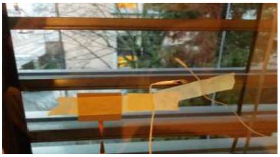
Figure 4.
In situ measurement set-up for the glazing U-value determination using HFM method. Reproduced from [44].
O’Hegarty et al. [45] stated that for a north-facing typical single-glazed window of a building located in the northern hemisphere, the in situ measured U-value using the average HFM method turned out to be almost 11% lower than the theoretical U-value. This measurement was carried out in winter with an average indoor/outdoor temperature difference of 7.2 °C. However, it was not explicitly mentioned whether the measured U-value was related just to the glazing part or if it included the entire window.
In another study conducted by Ficco et al. [46], the U-values of different building components were measured, including heavy walls, a light polystyrene insulating layer, and a double glazing system under different measuring conditions using an in situ HFM method. The authors found a temperature difference of less than 7 °C across the components, but not the heavy walls, and for the light insulation layer and the glazing system, the measured U-values (using the average analysis method) were very repeatable with meaningfully reduced uncertainties even in the short test duration (between 3 h and 12 h). It was found that the deviation between the measured U-values of the glazing system given by different types of HFM sensors and the value declared by the manufacturer was less than 5%. In another study carried out by Marshall et al. [47], the U-values of windows of a building fabric were measured using the in situ HFM method following ISO 9869-1:2014 [35]. However, no information was given regarding the windows’ configurations and whether the U-value was related to only the central part or the entire window. This study collected the results over a longer period (7 days) than that in the study by Ficco et al. [46], where the tests lasted less than 12 h, and only minor differences of about 3% were found between the standardized results and the measured results.
To determine the thermal and optical characteristics of a glazing system under real operational conditions, Goia et al. [24] developed a simple non-calorimetric method with relatively cheap equipment. This included sets of temperature sensors, heat flux meters, pyranometers, and a data acquisition system, which could be installed in real buildings or test cells. The proposed method was based on measurements of temperatures, heat fluxes, and solar irradiance values (for determining the g-value which is beyond the scope of this study). Figure 5 illustrates the energy flows and the parameters that were measured in the method. The U-value was evaluated by linear regression, conducted by the ordinary least squares method. With the help of night-time measurements (to avoid the impacts of solar radiation), the U-value was determined using the following equations:
where represents the reading of the heat-flux meter in () and and are the measured outdoor and indoor air temperatures in (°C), respectively. For the purpose of validation, the proposed method was adopted to evaluate the U-value of a case study, a conventional double-glazed unit, with known thermal characteristics and the data acquisition times in a range from one to two weeks each season. It was discovered that the in situ U-value could be determined with an accuracy range of ±10%–±15%, which is an acceptable degree of accuracy.
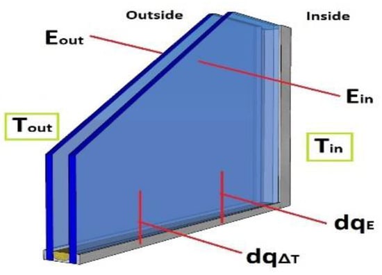
Figure 5.
Schematic representation of energy flows and relevant nomenclature: E_{out} (W·m−2) is the global (on vertical plane) impinging solar irradiance measured by a thermopile pyranometer; E_{in} (W·m−2) is the global (on vertical plane) transmitted solar irradiance into the room measured by a thermopile pyranometer; dq_{\mathrm{\Delta T}} (W·m−2) is the heat flux towards the interior due to the thermal gradient between outside and inside; dq_E (W·m−2) is the heat flux due to absorbed solar radiation. Adopted from Goia et al. [24].
In another study conducted by Park et al. [11], the U-value of an entire double-glazed window was determined using the HFM method. For this, the heat flux sensors, and the accompanying thermocouples were attached to the central part of the glazing at one point, to the edge of the glazing at six points, and to the frame part at three points (see Figure 6).
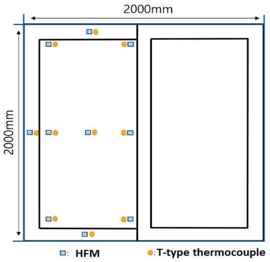
Figure 6.
Illustration of the measurement points for in situ HFM method. Reproduced from Park et al. [11].
The measurements were conducted over a 72 h time period and the U-value of each point on the window was determined according to the average method described in ISO 9869-1:2014 [35] (see Equation (7)). The U-value of the entire window () was calculated using the following equation:
where , , and represent the U-value of the central part, the edge part, and the frame part of the window, in (), respectively. , , , and are the area of the entire window, the center part, the edge part, and the frame part of the window, in (), respectively. Then, the result of the HFM method was compared against the standardized U-value obtained from a hot box measurement in the laboratory based on the Korean standard KS F 2278:2017 [48]. It was discovered that the U-value measured via the HFM method deviated by 5.9% from the standardized U-value. However, no more details regarding the temperature measurements and the impacts of the surface coefficients on the accuracy of the result were provided. In another study conducted by Aguilar-Santana et al. [40], the U-value of nine samples of one- and two-glazed static windows with different technologies and gas-filling materials was determined using an environmental chamber based on the average method explained by ISO 9869-1:2014 [35]. The authors reported that the U-values obtained via HFM showed good agreement compared with the results in the literature. It was concluded that in the vicinity of the window edges, higher U-values were measured than in the center part of the window due to the thermal bridges and the occurrence of convection motion in double-glazed samples containing a gas mixture in their internal cavities. It was stated that the scalability, accuracy, and adaptability of the HFM method listed it among the reliable in situ methods for the determination of a windows U-value. However, it was suggested that the difficulties in maintaining constant flow rates for quite a long period of time (72 h) and sensitivity to solar radiation could be considered as the drawbacks associated with this method.
It should be noted that, according to the literature review, the research studies that have adopted the HFM method mostly determined the windows’ U-values based on the average method under controlled conditions. Roulet et al. [49] conducted a study to compare the accuracy of the results derived from the average method and the standardized dynamic method for different building elements, including a double-glazed argon-filled window with coatings and a high insulation window with two inner selective plastic films. The authors concluded that for light elements such as windows, in the absence of solar radiation, the steady state could be reached quickly, and reliable results were therefore obtained with the average method and the dynamic method when applied to night-time recorded data. However, as far as daytime measurements were concerned, the average method came with very high dispersion and a very low mean value due to solar radiation interference in the long-term average. For the duration of the 6- 12- and 24 h measurement periods (but no longer), the dynamic method gave more reasonable results.
The in situ HFM method is based on point measurements; therefore, specifying the right points to which the sensors should be attached is not an easy task. This could also be seen as a drawback because the results obtained by a sensor only represent the properties of that specific point and do not reflect the properties of the entire surface [50]. In addition, several factors could affect the results obtained from the HFM method, including the errors of the equipment units and sensors, outdoor and indoor temperature differences, the presence of solar radiation, wind speed, adjacent heating or cooling devices, fluctuations in indoor and outdoor temperatures and heat flow during the measurement, thermal bridges, humidity, partial adhesion of sensors, and the homogeneity of the element under test [30,37,46,49,51]. Feng et al. [39] considered the in situ HFM to be a relatively expensive method that required a complex controller, data logger, and expensive heat flux sensors, along with the presence of an expert operator. The authors believed that one way to improve the buildings’ energy behavior could be to develop low-cost, easy-to-use, and, at the same time, reliable in situ methods to measure the thermal performance of envelope elements that even homeowners would be able to use to gain some idea of the thermal behavior of their building’s envelope. The authors’ suggested device is further discussed in Section 2.5. The summary of the HFM method with a focus on glazing systems is presented in Table 1.

Table 1.
Summary of the HFM method with a focus on glazing systems.
2.2. Guarded Hot Plate (GHP) Method
The guarded hot plate method is a steady-state measurement method that can be used to determine the U-value of middle-scale or small specimens (i.e., ideally, a square specimen fitted to 800 mm × 800 mm [40]). There are two types of guarded hot plate apparatus units, namely, the single-plate and double-plate apparatus. In the single-plate unit (see Figure 7 adopted from Tadeu et al. [52]), the test specimen is placed between an electrically heated plate (hot plate) and a cold plate. The hot plate is bordered by a guard heating system which is heated separately to the same temperature as the hot plate to minimize the heat loss to the exterior. In the double-plate method, the hot plate is embedded in the guard, but this time it is placed between two test specimens of the same size. When the electric system warms up the hot plate, note that the hot plate and the guard are the same temperatures; a unidirectional heat flow passes through the specimen(s) from the hot plate to the cold plate(s) perpendicular to the sample(s) surfaces. After reaching a steady state, the temperature difference over the sample(s) is measured using thermocouples [30]. Johra [53] stated that vertical pressure is needed to ensure good thermal contact between the test specimen and the plates.
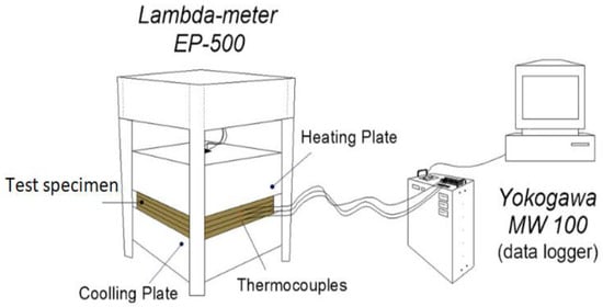
Figure 7.
Schematic of a single specimen guarded hot plate apparatus connected to a data logger. Adopted from Tadeu et al. [52].
Standard ISO 10291:1994 [54] (or EN 674:2011 [55] as stated by [56]) provided a method for determining the steady-state U-value of the central part of multilayer glazing using the guarded hot plate method [57]. According to the standard, and with the help of the apparatus, the surface-to-surface thermal resistance (R-value) of multiple glazing could be calculated via the following equation:
where , , , and , respectively represent the metering area in (); the average specimen hot side temperature, in (°C or K); the average specimen cold side temperature, in (°C or K); and the average powered supplied to the heating unit, in (W). Then, the U-value of the multiple glazing can be determined using Equation (5). It should be noted that all the measurements should be carried out in an upright position since the standard does not consider inclined glazing samples [58]. The values of and for a normal multilayer glazing without low-E coating on the surface are assumed to be 23 () and 8 (), respectively, which are slightly different from the standardized values that are used for the HFM apparatus. However, a multilayer glazing with a low-E coating on its internal surface, can still be calculated using Equation (7).
As far as the accuracy of the GHP method is concerned, standard ISO 8302:1991 [59] states that the expected accuracy at room temperature and for the full temperature range would be expected to be between 2% and 5%, respectively, which shows a high level of accuracy [30,60]. It is stated that since this method is based on steady-state measurements, there must be sufficient time for the apparatus and the specimen to reach the thermal equilibrium, but the time needed may vary from several minutes to several days, based on the apparatus, the specimen, and their interactions [59]. Thomas and Zarr [61] highlighted the protracted time required to complete each test using the GHP method.
In a study conducted by Ghazi Wakili et al. [57], the U-values of the central part of triple-glazed low-E coated insulating glass units with argon filling from five different suppliers were measured by a guarded hot plate apparatus. The apparatus used for the experiment was equipped with an electromechanical control unit, which, after the installation of the sample, could rotate the whole apparatus, including the samples, from a horizontal into a vertical position. All measurements in the study were conducted in the vertical position so as to be in line with the requirements of EN 674:2011 [55]. The results of the experiments were then compared with the values declared by the manufacturers which all were about 0.6 (). The comparison showed that, except for one sample, there were deviations between the experimentally measured and the declared U-values. The reasons for the deviation were mostly attributed to the degradation of the low-E coatings in the cavities. The authors also claimed that it would be possible to explore the linear thermal transmittance (Ψ-value) of the edges of the glazing unit, the sealing, and the spacer (excluding the frame part) () using a guarded box. For this purpose, each glazing sample was tested twice, once for the whole glazing unit and then after it had been divided into two parts and glued together along the longest side (see Figure 8). The Ψ-value was determined through the following equation:
where , , , , and , respectively represented the total heat loss through the single unit, the total heat loss through the two-glued double units, the temperature difference over a single unit, the temperature difference over the two-glued double units, and the length of the metering area. The authors also suggested the use of an additional insulation (EPS) belt around the samples to prevent the circulating air inside the GHP from impacting the measurement results. It was also mentioned that the specimen needed to be treated in a chamber to reach the standard temperature before being placed in the apparatus. Standard ISO 10291:1994 [54] defined a mean temperature of 10 °C for the specimen and a maximum temperature difference of 15 °C through the sample thickness. In addition, the authors highlighted the importance of the flatness of the sample to the accuracy of the results; it was mentioned that the gas compression in the cavity (because of lower temperatures) could lead to a dishing effect.
Figure 8.
Schematic of the two glued samples of triple-glazed units of 400 mm × 800 mm and the temperature sensors. The door can only be opened in a horizontal position. Reproduced from Ghazi Wakili et al. [57].
Sánchez-Palencia et al. [56] pointed out that in ISO 10291:1994 [54], similar to standards EN 673:2011 [62] and EN 675:2011 [31], the internal and external surface heat transfer coefficients are assumed to be fixed values, although these values might differ depending on the environmental conditions, the geometry of the building, and the position of the windows. Therefore, similar to the HFM method, if the U-value is used for the design stage or if the U-value of existing glazing needs to be evaluated, the standardized surface heat transfer coefficients can change according to the case conditions.
Tadeu et al. [52] used the GHP apparatus to experimentally validate a boundary element model (BEM), which was formulated in the frequency domain to study the dynamic behavior of linear thermal bridges (see Figure 7). For experimental measurements, a pre-conditioned multilayer system (with a set-point temperature of 23 ± 2 °C and 50 ± 5% relative humidity) was placed in a single-specimen guarded hot plate apparatus and exposed to an unsteady heat flow rate. First, the apparatus maintained a mean temperature of 23 °C in the test specimen and a 15 °C temperature difference between the heating and the cooling units. Therefore, the temperature of the top multilayer surface (in contact with the heating plate unit) rose, while the temperature of the bottom multilayer surface (in contact with the lower plate) dropped. The energy input was maintained until stability was achieved, and there were no temperature variations at the multilayer interfaces. Once stability was reached, the system stopped heating and cooling so the temperatures of the multilayer systems could return to their initial states. The temperature variations at each interface layer were measured by thermocouples, which were connected to a data logger system to record the data (see Figure 7). The test took 16 h, and its results were later compared with the numerical results based on the BEM. The comparison showed that the BEM solutions agreed with the experimental ones. This study showed that although the primary goal of the GHP method was to analyze the thermal properties of the samples in a steady-state condition, it could also be used to study the dynamic behaviors of the samples or to validate the numerical methods when studying the dynamic behavior of different products. In the future, this approach might also be applied to glazing systems to analyze their behavior under dynamic conditions with GHP apparatus. A summary of the GHP method with a focus on glazing systems is presented in Table 2.
Table 2.
Summary of the GHP method with a focus on glazing systems.
2.3. Hot Box (HB) Method
The hot box method has been widely used for the thermal testing of full-scale homogeneous and non-homogeneous [3,24] building components mostly at a steady-state [30] and sometimes at dynamic conditions [25,63] in the absence of solar radiation and air leakage effects [64]. Several standards have been drafted for this method, e.g., standards ISO 8990:1994 [65], widely used in Europe, the American ASTM C1363-05:2005 [66], the Russian Gost 26602.1-99 [67], and the Korean KS F 2278 Standard [48]. The first three standards describe the design requirements for the HB apparatus, the measurement technique, and the test procedure required to obtain the U-value [3,68]. The main purposes of those standards are all the same, which is to create a temperature difference in steady-state conditions across the test specimen placed between a room warmed by a heating unit (simulating the indoor condition) and a cold room connected to a cooling unit (simulating the outdoor condition). The specimen is also surrounded by a panel with known thermal properties. ISO 8990:1994 [65] and suggested temperatures of 20 °C and 0 °C for the warm and cold side, respectively, whereas Asdrubali and Baldinelli [3] report that the American ASTM C1363-05:2005 [66] and the Russian Gost 26602.1-99 [67] specified different levels, specifically for the cold side which are −17 °C and −20 °C, respectively. The results obtained from ISO 8990:1994 [65] and ASTM C1363-05:2005 [66] are expected to be similar because they have almost the same procedures and methodology for defining heat exchange. In both standards, the sample that was made up of different components was treated as a single black box; therefore, only the total heat transfer through the sample was considered for U-value determination, while the Russian Gost 26602.1-99 [67] attempted to take the thermal properties of each component of the sample into consideration to determine their weaknesses and strengths, this caused the procedure to be time-consuming and more complicated, especially for strongly non-homogeneous specimens [3].
Two main types of hot box apparatus were built according to standard ISO 8990:1994 [65], these being the guarded hot box (GHB) and the calibrated hot box (CHB). Both devices are suitable for testing full-scale vertical and horizontal specimens (such as walls, ceilings, floors, and vertical and sloped window systems) [3,30]. For the horizontal and sloped solutions, the hot box needed to accommodate the exact position of the specimens. The guarded hot box test device was made up of three main components, namely, a guard box, a metering box, and a cold box [30] (see Figure 9a). The guard box surrounds the metering box, and both are equipped with circulating fans to maintain airspeed and temperature uniformity. The metering box’s open side was pressed against the test specimen, which was then placed between the cold box and the guarded metering box [21]. To prevent any heat loss from the metering box to the guarded box and to ensure that the total heat supplied to the metering box was crossed the test specimen in a direction perpendicular to its faces, their temperatures should be the same [21,25,30,69]. Prata et al. [25] stated that the guarded HB apparatus would not require calibration; however, unlike the calibrated HB apparatus, its relatively modest measuring area meant that larger specimens could not be tested.
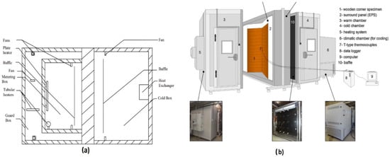
Figure 9.
Schematic of HB apparatus. (a) A guarded HB apparatus, reproduced from Ghosh et al. [69]; (b) A calibrated HB apparatus with a wooden specimen under test, reproduced from Prata et al. [25].
The calibrated apparatus consists of two main parts, the metering box (the hot room) and the cold box, which are both made from insulation materials and prevent heat transfer between the device and the external environment [25,30,70] (see Figure 9b). The external environment should be ventilated to maintain the desired temperature and to keep errors associated with the apparatus to a minimum; however, its temperature does not necessarily need to be the same as the hot room [63]. The test specimen was placed in the aperture of a surrounding panel facing the hot box on one side and the cold box on another side. The chambers were equipped with fan systems to prevent thermal stratification [71]. The measurements were taken once the temperature in each box was stable. To determine the heat loss through the metering box walls, heat transfer through the surrounding panel, and the flanking losses, several calibration tests needed to be carried out under a wide range of environmental temperatures before the main test. This required the help of calibration panels with a known thermal resistance range [25]. With the knowledge of the box and marginal heat losses, the amount of heat that passed through the test specimen could be quantified [30].
The main difference between the guarded hot box method and the calibrated hot box method was that the former did not need calibration. It was discovered that the guarded hot box could provide more accurate results and has shown greater flexibility in terms of the boundary conditions adjustment (e.g., temperature difference range) [21]. However, unlike the calibrated hot box apparatus, the guarded hot box could not be used for large specimens or singular solutions, including corner walls, because of its modest measuring area [25]. Both the guarded and calibrated hot box units are regarded as expensive equipment units [30].
In addition to the above-mentioned standards, there are two significant standards that have been specifically prepared to determine the U-value of fenestration systems using the HB method; they are standard ISO 12567:2010 [72] (mostly used in Europe) and the American ASTM C1199:2014 [64]. In both standards, the measured U-value (, in ) was obtained by dividing the density of the heat flow rate through the specimen, in (), and by the temperature difference between the two sides of the specimen, in (K). However, in ASTM C1199:2014 [64], the temperature difference between the two sides of the specimen refers to the average air temperatures, while in ISO 12567:2010, it refers to the environmental temperatures (including the radiation impact). For the purpose of rating and comparing the results of the HB methods (followed by different standards) with each other and/or with the theoretical and simulation results, the U-value measured by the HB method needed to be standardized by correcting them with the standardized total surface thermal resistances (for ISO 12567:2010), or with the standardized total surface heat transfer coefficients (for ASTM C1199:2014) [73].
ASTM C1199:2014 introduced two methods for standardizing the measured U-value; these are the calibration transfer standard (CTS) method and the area weighting (AW) method. To determine the surface heat transfer coefficients on the fenestration product, the CTS method required the calculation of equivalent surface temperatures from the calibration data, while the AW method required the directly measured surface temperatures on both sides of the test specimen (see Figure 10). The standardized surface heat transfer coefficient for the room side () and the weather side () considered by this standard are 7.7 () and 30 (), respectively. More details regarding the measurements, calibration and standardization of the measured U-value can be found in the standard.
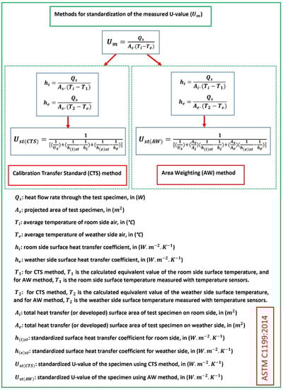
Figure 10.
Summary of the standardization of the measured U-value following the standard ASTM C1199:2014.
As far as the standardization of the measured U-value using ISO 12567:2010 is concerned, the standardized value of the total surface thermal resistance, , for windows was assumed to be 0.17 (). Figure 11 summarizes the procedures that should be followed to obtain the standardized U-value () of the glazing based on ISO 12567:2010. More details regarding the measurement, calibration and standardization process can be found in the standard.
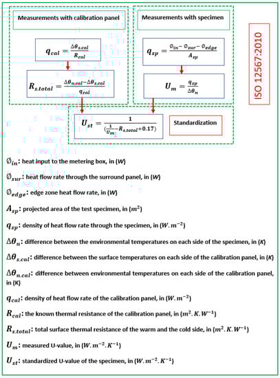
Figure 11.
Summary of the standardization of the measured U-value following method standard ISO 12567:2010.
Desjarlais and Zarr [73] stated that the standardization of the measured U-value using the HB method might result in a greater uncertainty of the results since it requires measuring and calculating more values (based on the standard that is followed). The authors discussed one alternative solution, which was to introduce variable local heat transfer coefficients or thermal resistances for the cold and warm side surfaces and glazing cavity, so the results of the simulations, theoretical calculation, and other methods could be directly compared with the actual measured U-values from the HB method.
In a study on the impacts of the distance between the pillars in vacuum glazing on the U-value of the window, conducted by Cho and Kim [74], it was highlighted that one of the benefits of the hot box method was that the edge effects of the glazing would be considered in the window U-value determination. However, in simulation tools (in this case, WINDOW), the edge impact of the vacuum glazing caused by its insulation condition was not considered, which resulted in differences between the experimental and simulation results. In addition to the entire window’s U-value determination, researchers have tried to use the hot box method to evaluate the U-value of the frame part. For instance, Lechowska et al. [75] used a hot box device to evaluate the U-value of three types of PVC window frames based on EN 12412-2:2003 [76]. Three frame units with insulation panel fillings were mounted into the surrounding panel in the hot box, and the U-value of the frames was obtained using the following equation:
where , , , , , and represented the measured total U-value (), the total area (), the environmental temperature difference (K), the thermal conductance of the insulation panel filling (), the surface temperature difference of the insulation panel filling (K), the area of the insulation panel filling (), and the area of the frame, respectively. The results of the measurements were then compared with a CFD model, which was developed by a two-dimensional simulation (Ansys Fluent), and a maximum deviation of 3.3% between the simulation and the measurement results were found.
In another study conducted by Kim et al. [77], the impacts of PVC and aluminum frames on the energy performance of different types of window systems were investigated using a hot box apparatus. The windows were classified as sliding, double cut-up sliding, quadruple cut-up sliding, fixed window, fixed window with a project, and project window. In the study, the U-values of the glazing sections were determined prior to the hot box test with the help of the software WINDOW. In the next step, by conducting hot box tests, the U-values of the entire windows were obtained, and finally, the U-values of the frame part was calculated using the following equation:
where is the U-value of the frame, and are the U-values of the window and glazing, respectively. , and are the areas of the window, glazing, and frame in (), respectively. It should be noted that in this study, the frame part of the window included the performance of the spacer because the impact of the spacer and the associated linear thermal bridges could not be measured separately.
Grynning et al. [78] adopted the HB method to investigate the impacts of integrated (in-between pane) Venetian-style shading units on the U-value of several windows with 2-, 3-, and 4-pane glazing units. The measurement results were then compared with a numerical simulation using the THERM/WINDOW simulation tools. The comparison revealed that numerically simulated U-values were lower than the measured U-values. The authors felt that there could be several reasons for the disparity, including the difference between the real characteristics of low-E coatings and those the manufacturer acknowledged, thermal bridging effects that were not considered in the simulation, and the probable occurrence of some air leakage during the HB tests. The first two reasons are related to the simulation method’s weaknesses, while the last is related to the experimental method’s weaknesses. Banionis et al. [79] investigated the impacts of the indoor and outdoor temperature difference on the U-value of insulated double and triple-glazing units with low-E coatings using a guarded hot box apparatus. In the study, in addition to the windows’ U-values, the U-value of the central part of the glazing was measured using additional temperature sensors and a heat flux meter attached to the central part of the glazing. The temperature on the warm side of the hot box was kept at 20 °C, but for the cold side, three different temperatures, 0 °C, −10 °C, and −14 °C were set. The results of the study showed that as the cold side temperature dropped from 0 °C to −14 °C, the U-value of an entire window increased by approximately 9–10%, while the U-value of the central part of glazing units increased by approximately 14–15%. Based on the results of the measurements, the authors concluded that the U-value of the insulated glazing units with gas fillings and low-E coatings would depend on the outdoor temperatures; therefore, to predict the heat loss through windows and buildings’ energy consumption more accurately, it would be more reasonable to introduce designed U-values for windows based on the climate zones, instead of using the standardized declared U-values.
In real situations, building elements are in dynamic conditions and, therefore, to obtain more accurate results regarding the thermal performance of the building elements, studies would have to be conducted in real dynamic conditions [68,80]. The hot box was standardized to work in stationary conditions. However, some research studies have tried to apply hot box methods to investigate the thermal behavior of some building wall specimens with and without thermal bridges and in dynamic conditions [25,81,82,83]. They used different techniques, including sinusoidal excitations in the cold chamber to vary the cold side temperatures and impulsive solicitation. However, the literature review showed that research into the dynamic thermal behavior of window systems using hot box methods is not receiving enough attention.
As far as the reliability and accuracy of the HB method are concerned, the literature regards it as an accurate and reliable method for the U-value determination of large-scale systems in such a way that its results could be considered a reference with which the results of other experimental and theoretical methods could be compared for the validation purpose [3,30,84]. Baldinelli and Bianchi [23] also stated that for a window manufacturer to achieve high-performance certified products, and test on an experimental hot box set-up would be more appropriate than other methods.
In terms of the measurement duration, standard ISO 8990 does not mention any specific requirement, but it does say that the required time to reach stability for steady-state tests depends on factors such as thermal resistance, thermal capacity, surface coefficients, presence of mass transfer and/or moisture redistribution within the sample, and the apparatus. However, generally, the HB is known for its relatively long measuring time [30], usually several days [85]. It should be noted that the measurement time could also depend on the standard chosen to follow the adaptation of the HB method [3]. The HB method, with a focus on glazing systems, is summarized in Table 3.
Table 3.
Summary of the HB method with a focus on glazing systems.
2.4. Infrared Thermography (IRT) Method
In the infrared thermography (IRT) method, the infrared radiation emitted by the objects is captured and converted to electrical signals, which enable the images to be generated with the distribution of the surface temperatures of the objects and with the help of the Stefan–Boltzmann law. IRT could be divided into two categories, namely, qualitative and quantitative IRT [30]. In the qualitative IRT, the main focus was usually on identifying surface imperfections in building elements, moisture issues, air leakage, and thermal bridge locations. IRT can also be used as a supplementary tool to help find locations without any defects or non-homogeneities for attaching the heat flow meters [50,86,87,88]. The quantitative IRT can be used as a non-invasive method of investigating the building elements’ thermal performance, e.g., the Ψ-value of junctions, the temperature distribution of elements’ surfaces, and the U-value of the elements [30,88,89].
Regarding the thermal bridges in the building envelope, as O’Grady et al. [90] stated, most of the studies investigated single linear thermal bridges with moderate temperature gradients separately from each other, thereby ignoring their impacts on each other. With the help of quantitative IRT, Asdrubali et al. [91] defined heat loss through thermal bridges with a factor indicating how the heat loss through a building element would increase as a result of thermal bridges. The quantified thermal bridging heat loss was determined by multiplying the factor by the U-value of the plain component, which was then measured by a heat flow meter (HFM). The proposed method was validated on a thermal bridge between a window frame and glazing in laboratory conditions. Based on that approach, O’Grady et al. [90] tried to use indoor IRT techniques to simultaneously investigate the multiple parallel thermal bridges with large gradients in the surface temperature distribution. For this purpose, two specimens containing parallel thermal bridges created by square hollow steel (SHS) sections (the distance between them was different for each specimen) were tested. In addition, two window configurations (one with a wooden frame and one with a PVC frame) were studied using IRT, with the whole installed window considered as a single unit and the total heat loss due to the window system (including heat loss through the glazing, frame, the connection between frame and glazing, and heat loss around the window due to installation) was quantified. The qualitative IRT showed that the distance between the thermal bridges would determine the degree of interaction between them. The interaction between the parallel thermal bridges, which were close to each other, was so significant that they acted in similarly to a single thermal bridge (see Figure 12). For the square hollow steel (SHS) sections, the IRT measured thermal bridging heat losses, in (), and the Ψ-values, in (), were compared with the values obtained from hot-box measurements. For the windows, the IRT measured heat loss through thermal bridges, in (), and the so-called M-values, in (), were compared with the values given by hot-box measurements. The comparisons showed deviations of less than 10% between the equivalent values, which was assumed a good agreement.
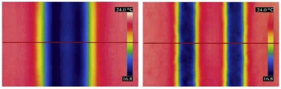
Figure 12.
Sample IR images for specimens with parallel thermal bridges created by square hollow steel (SHS); two parallel thermal bridges positioned at a distance apart smaller than the specimen thickness (left), and two parallel thermal bridges positioned at a distance apart greater than the specimen thickness (right). Reproduced from O’Grady et al. [90].
Baldinelli and Bianchi [23] used IRT to compare the experimental and simulation results regarding the U-values of two types of window systems. The IR images showed the surface temperature distribution on the warm side of the test specimens and enabled a comparison with the surface temperature distribution derived from the numerical analysis. The IR image revealed that the surface temperature distribution along the windows was not symmetrical, and the upper parts showed higher temperatures which were attributed to the air stratification effect, while the simulation thermal image was quite symmetrical, meaning that the air stratification was underestimated by the simulation. As far as the U-value determination using quantitative IRT techniques was concerned, the comprehensive literature review conducted by Kirimtat and Krejcar [92] reported that many studies used the IRT method to evaluate the U-values of opaque elements, such as internal and external walls, roofs, bricks, plasters, and insulation materials (see Table 1 in [92]). However, only a few papers were found that dealt with the thermal performance of windows, and, more specifically, only one reference for the window’s U-value assessment using IRT techniques was mentioned. Lucchi [93] stated that there would be some difficulties applying IRT to glazing thermal performance determination since IR images of a glazing system would be very sensitive to its surroundings. There are several factors that could affect the accuracy of IRT results, including the glazing emissivity, air temperature, environment temperature, atmospheric temperature, relative air humidity, the distance from the object, and the specular reflections of surrounding objects [23,93]. In addition, the investigated object must be in a steady-state condition to be free of disturbing influences, which could be difficult in real conditions (in situ) because building glazing systems are exposed to dynamic environmental conditions [94]. Therefore, Lucchi [93] pointed out that indoor IRT surveys under strict boundary conditions (i.e., the use of high emissivity materials as reference ε-values, with uniform wind velocity and temperature gradient of 15 °C across the glazing) could give more accurate results. Boafo et al. [95] received help from an IRT technique to compare the performance of two different window systems (before renovation and after) and their thermal bridges based on the temperatures of the window surfaces; however, they did not evaluate the window’s U-values using IRT.
Fokaides and Kalogirou [96] used IRT to evaluate the overall U-values of building envelopes, including the windows. However, the authors do not present a detailed method describing the window’s U-value assessment with IRT. It was concluded that IRT-measured U-values were at an acceptable level in the range of 10–20%, while the roofs and windows showed higher deviations than the other building elements because of the thermal inertia effects, which could not be controlled. Maroy et al. [97] investigated the reliability of the U-values for insulated glazing units using IRT techniques. It was found that the evaluation of the thermal performance of glazing systems based on their surface temperatures was not straightforward, either in the laboratory or in situ (for both inside and outside measurements). The biggest issue with glazing systems was determining the accurate heat surface coefficients, which were easily affected by wind and indoor and outdoor heating elements. The authors concluded that the IRT survey could be adopted to differentiate between good and poor glazing units, but the accurate glazing unit’s U-value (or R-value) determination might not be achievable even if strict boundary conditions (i.e., cloudy conditions, the high-temperature difference over the sample, etc.) were applied. Meanwhile, in a recently published study conducted by Park et al. [11], IRT was used to calculate the U-value of a double-glazed window of an existing house. The study was based on the standard ISO 9869-2:2018 [98], while the standard was devised to determine the opaque building elements’ U-value. In order to adopt the standard method for a window unit, a blackbody was built to correct the emissivity and reflectance so that the emissivity was assumed to be one and the reflectance zero. Then, the surface temperatures of the center of the glass, the edge of the glass, and the frame were measured with an IR camera (see Figure 13). By considering two different values for the internal surface heat transfer coefficient, = 9.09 () from the Korean energy-saving design standard and = 7.69 () from ISO 6946:2017 [99], two scenarios were created, and the total U-value of the window was calculated for each scenario using the following equation:
where , , and represent the total heat transmission rate for the window, the surface heat transfer coefficient, and the area of inner window, respectively. The subscripts c, e, f, and t mean the center, the edge, the frame, and the entire window, respectively. , , and are equal to , , and , respectively. , represent the indoor and outdoor temperature, respectively.
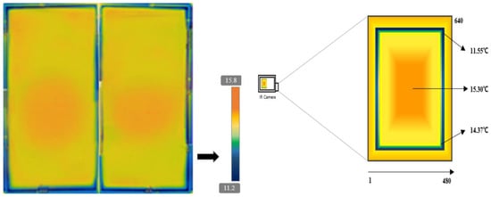
Figure 13.
Window surface temperatures using an IR camera [11].
Finally, the IRT-measured U-values of the entire window for both scenarios were compared against the U-values obtained from the Korean KS F 2278 Standard [48] (using a hot box device in the laboratory) and heat flow meter method. The comparison showed that the result of the first scenario, in which the internal surface heat transfer coefficient was = 9.09 (), was only 3% different from the standard U-value. The deviation of the results for the second scenario (with = 7.69 ()), and the heat flow meter method (with the average method) from the standard U-value were reported to be 11.8% and 5.9%, respectively. It was concluded that the IRT could be considered a reliable method for determining a window’s U-value. Finally, the authors suggested further investigation of the IRT-measured U-values with the measured surface heat transfer coefficients instead of the values reported by standards. It is worth mentioning, too, that the fact that the IRT-measured U-value was closer to the standard value does not necessarily show that it was more accurate than the heat flow meter result. As previously mentioned, the standard values usually involve some simplifications and assumptions which may not be true for all conditions.
Recently, combining the UAV (unmanned aerial vehicle)-assisted thermal imagery with machine learning techniques to estimate the U-value of building envelopes has attracted researchers’ attention. This approach has the potential to revolutionize the process of the thermal assessment of building elements since it is a non-destructive method giving surface temperature data for a large inspection area in a short time remotely without any need to manually analyze the thermal images to estimate U-values [100,101]. The study conducted by Sadhukhan et al. [100] revealed that the U-values of windows estimated by machine learning techniques through analyzing the UAV-assisted thermal images differentiated from the performance of single- and double-glazed windows. This means that, for a building with several windows, it could be possible to evaluate the impacts of windows on the building’s energy performance. However, the U-values were found to be sensitive to the outdoor conditions with some discrepancies from theoretical values. This approach is at its initial stage and is expected to reach more attention in the future.
Table 4 summarized the main findings for the quantitative IRT method with a focus on glazing systems.
Table 4.
Summary of the IRT method with a focus on glazing systems.
2.5. Developed Rapid U-Value Meter Tools
Some rapid and easy-to-use U-value (and g-value) meter tools have been developed by researchers in recent years. These were claimed to be useful for acquiring some knowledge of the energy performance of existing windows in real conditions [102]. In a study by Pekkala [103], an instrument called a rapid U-value meter (see Figure 14) was used to rapidly measure the U-value of five windows of the same type but different sizes. However, some other supplementary equipment units, such as a wind speed meter, thermocouples, a pyranometer, a thermal imaging camera, and a data logger system, were also useful. The basic principle was to place the rapid U-value meter at different measuring points on the inner surface of the glazing. The components of the rapid U-value meter are shown in Figure 14. Temperature sensor number 1 (under the instrument), covered with thermal insulation (number 4), measured the temperature. Another temperature sensor (number 2) simultaneously measured the temperature of the undisturbed area. The decline in temperature at the point of temperature sensor 1 because of the insulation could be recognized by the control system (number 5), which triggered the electrical heater (number 3) to compensate for the temperature drop. In that way, the temperatures at sensors 1 and 2 could become equal. The power () required to keep temperature sensors 1 and 2 at equilibrium was displayed on the instrument in (), which could be converted to (). Then, based on the heating power, the inner surface temperature, , in (°C), and the outside air temperature, , in (°C), and the U-value of the measuring area could be achieved through the following equation:
where , and represent the area of the instrument, in this case, 0.01, the internal surface resistance, which was assumed to be 0.13 (), and the external surface resistance, which was assumed to be 0.04 (). It was also mentioned that the additional heat due to electronics (in this case, 5 ) and the impact of solar radiation could also be added to in the equation. The author mentioned that when it came to the U-value measurement of the center part of an existing window’s glazing, in the 5–6 h of night-time measurements, reliable results close to the standardized values (with a maximum deviation of ±5%) could be obtained. However, this instrument could not be used to directly measure the U-value of the frame part and the linear thermal bridges between the glazing edges and the frame. This could be due to a rapid change in temperature in the horizontal direction, requiring the instrument to be well aligned vertically so that both temperature sensors could be placed in the same temperature direction, as well as the fact that there was not usually enough space to place the instrument correctly on the frame and edge part of the window. These issues would result in unreliable values. Thus, with the combination of theoretical calculations based on the technical data relating to the frame part and linear thermal bridges (using the manufacturer’s data) and the U-value of the center part of the glazing measured by the rapid U-value meter, the U-value of the entire window could be obtained.
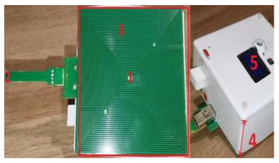
Figure 14.
Components of a rapid U-value meter. Reproduced from Pekkala [103].
Feng et al. [39] introduced a portable and relatively cheap tool for in situ measurements of the thermal and optical performance of the glazing system of existing buildings (see Figure 15). The tool could help the building owners or occupants to find out about the energy performance of their buildings’ windows before undertaking any energy efficiency measures or renovation. Using the Arduino platform and low-cost sensors (including low-cost and small-dimension digital elements, mainly including luminosity sensors, phototransistors, temperature sensors, surface temperature sensors, and a display screen), the tool was specifically designed to measure the glazing properties, including the U-value of the center part of the glass, the solar transmittance, and the visible light transmittance. Without the need to use an expensive heat flux sensor, and considering the fact that in a steady state, the heat flux intensity would be equal through the different layers, by only measuring the surface temperatures of the glazing and a supplementary object with pre-measured thermal resistance, (), the U-value () of the center part of the glazing could be calculated through the following equations:
where , , , and represent the surface temperature of the object exposed to indoor air (°C), the temperature of the interface between the object and the glass (°C), the temperature of the outer surface of the glass (°C), and the area of the surfaces ().
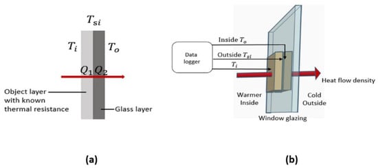
Figure 15.
(a) Heat transfer through the multi-layered surfaces; (b) The measurement setup for the instrument. Reproduced from Feng et al. [39].
The authors mentioned that the U-value of the center part of the glazing displayed by the tool was measured under a so-called quasi-steady state. In fact, the time expected for the system to be stable was about 30 min. When the difference between the average and maximum U-values was smaller than 5%, it was assumed that the expected quasi-steady state could be reached, and the average U-value would be displayed.
To validate the accuracy of the measuring tool, in late October-early November, three measurement experiments were carried out on an existing double-pane window (two 6 mm clear glass panes with an air gap) in absence of solar radiation (to comply with ISO 9869-1:2014 [35]). Table 5 summarizes the results of the three measurements knowing that the U-value of the center part of the glass declared by the manufacturer was 2.97 (). The results showed that the accuracy of the results of the measuring tool was between 6.1 and 21.6% and, as mentioned by Soares et al. [30] and ISO 9869-1:2014 [35] regarding the in situ U-value measurements, the smaller the temperature difference between the indoor and outdoor, the less accurate the results. In addition, it could be seen that the time needed to reach the so-called quasi-steady state for the case with lower indoor-outdoor temperature differences was relatively longer. The authors stated that the weather conditions (including the wind speed), solar radiation, indoor-outdoor temperature differences, stability, frost, and condensation would affect the accuracy of the results measured by the tool.
Table 5.
Summary of the results of the three measurements of an existing double-pane window using the rapid U-value meter. Conducted by Feng et al. [39].
To sum up, these relatively cheap and easy-to-use instruments used by Pekkala [103] and Feng et al. [39] could be very useful for evaluating the thermal performance of existing windows before energy retrofitting measures. However, more research on these so-called rapid U-value meters seems necessary, first, to investigate their applicability and accuracy for different glazing systems under different boundary conditions, and second, to promote them so that they could be used to evaluate the U-values of entire windows (not only the center of the glazing part).
3. Critical Review
This review paper has studied the main experimental U-value assessment methods for window systems, including the heat flow meter (HFM) method, the guarded hot plate (GHP) method, the hot box (HB) method, the infrared thermography (IRT) method, and the so-called rapid U-value meter method. Table 6 summarizes the main advantages and disadvantages of each of the reviewed methods and provides the possibility of comparing them with each other. It can be seen that the HB method allows measurements under a wide range of controllable boundary conditions representing different weather conditions with reliable and accurate results. It also allows the U-value of an entire window to be measured considering all the involved complex heat transfer mechanisms that are usually simplified in theoretical methods. However, this method, together with GHP and HFM apparatus methods can only be adopted in the laboratory. In order to measure the U-value of windows/glazing systems onsite, HFM sensors, the IRT method, and the so-called rapid U-value meters tools could be used. Table 6 shows that although the HFM sensors method could provide reliable U-values of the existing windows, the cost of the equipment is usually high. In addition, to evaluate the U-value of the entire window this method requires the use of several heat flux sensors simultaneously, which, in turn, increases the cost of the test. As far as the applicability and reliability of the IRT method for determining the U-value of a window are concerned, the literature review revealed opposite attitudes. As discussed previously, Maroy et al. [97] limited the applicability of the IRT method to differentiate between good and poor glazing units, while Park et al. [11] considered this method to be a reliable one in order to obtain the U-value of a window. Therefore, more research into the applicability of the IRT method in this area is needed. In addition, its equipment is expensive, and adopting the method requires special expertise. The most important issue with the so-called rapid U-value meter tools is the lack of research and the fact that most of them can only measure the U-value of the central part of the glazing (they cannot measure the U-value of the entire window). The literature review revealed that the amount of research dealing with this type of tool is still limited. However, once their reliability and accuracy of them are confirmed, they can be widely used since they are cheap, easy to use, and fast, providing useful information needed for window retrofitting measures.
Table 6.
Comparison of the reviewed methods for determining the U-value of a window.
It can be said that there are two main goals for determining a window’s U-values. The first is to compare different new products with each other in a reliable way so the designers can choose their desired products with more confidence. The second goal is to assess existing windows’ thermal performance in a cheap and reliable way before embarking on any energy retrofitting measures.
To accomplish the first goal, it is necessary to identify reliable laboratory methods that are capable of producing different boundary conditions so that the U-value of the products (especially the ones with low-E coatings) under different boundary conditions can be evaluated. As discussed previously, the U-value of a window can be affected by outdoor/indoor conditions (e.g., temperature, wind speed, etc.) [79]. To obtain the second goal, it is necessary to identify the most suitable method in terms of reliability, cost, test duration, and ease of use.
To achieve the above-mentioned goals, the authors of this paper proposed a comprehensive study that provides the possibility for a fair comparison of different new window products and even different laboratory and in situ methods. Figure 16 illustrates the proposed comprehensive approach.
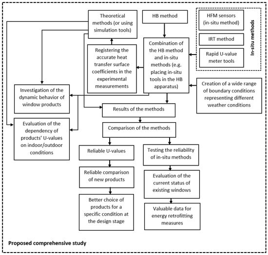
Figure 16.
The comprehensive study proposed by the authors.
The proposed study suggests the combination of the HB method as a reliable laboratory method and the reviewed in situ methods (HFM, IRT, and rapid U-value meter tools) under different boundary conditions for a wide range of window systems. Accurate registration and the introduction of the boundary conditions of the tests to the simulation tools (or theoretical methods) allow for a fair comparison between the measured and the simulated (or calculated) U-values. In addition, there is a possibility to evaluate the dynamic performance of window systems following the methods reviewed in this paper or in newly proposed ones. This comprehensive approach could also shed new light on the applicability and accuracy of the IRT method and the U-value meter tools, which would be helpful for energy retrofitting measures. In addition, such a comprehensive study would specify the U-value of a wide range of products under different weather conditions, thus leading to a better choice of products at the design stage.
Last but not least, researchers in the future may consider including other experimental methods, such as GHP and HFM, methods in the proposed study in such a way that their boundary conditions will not be limited to the standardized ones.
4. Conclusions
Windows are responsible for a considerable amount of energy needs in all types of buildings. Therefore, to have energy-efficient buildings, it seems inevitable that the energy performance of windows should be improved. One of the most important parameters indicating the energy performance of window systems is thermal transmittance (U-value). This value should therefore be assessed as accurately as possible before embarking on any energy efficiency measures.
This review paper has studied the main experimental U-value assessment methods for window systems, including the heat flow meter (HFM) method, guarded hot plate (GHP) method, hot box (HB) method, infrared thermography (IRT) method, and the so-called rapid U-value meter tools. The first step was to try and identify the standardized procedures for each method, then to analyze the advantages, disadvantages, and new possibilities provided by researchers which complemented the standardized methods.
The review showed that some useful methods, including the in situ HFM method and quantitative IRT method, could be of great help when it comes to assessing the performance of windows in real conditions; however, no standardized procedure specifically dealing with window systems was found. While most attention has been paid to the opaque elements with quite different characteristics from those of window systems, this gap could cause difficulties for researchers in terms of the comparison and validation of their own proposed methods. It was also found that the investigation of the dynamic thermal performance of window systems for most of the above-mentioned methods has received less attention, while in real situations, the window systems are exposed to dynamic conditions. Therefore, this fact can be taken into consideration in future studies by adopting and improving the dynamic analysis of a window’s U-value.
Another important point that was discussed in many of the reviewed papers was the difference between the standardized boundary conditions and real ones while assessing the thermal properties of windows. It was repeatedly stated by the authors that although the standardized boundary conditions provide the opportunity to compare different window systems, they may not necessarily represent the actual behavior of the products in different geographical locations, climates, and orientations. As Kuhn [104] stated, the U-value is not a material constant and can be influenced by several boundary conditions, such as the external and internal heat transfer coefficients, wind conditions, internal and external temperatures, etc. Therefore, it could be useful to make the standardized methods and their proposed conditions more flexible so that they can be used to study the behavior of window systems based on different boundary conditions.
In the end, the authors of the paper proposed a comprehensive approach and provided the possibility for a fair comparison of different new window products and even different laboratory and in situ methods under a wide range of boundary conditions representing different weather conditions. Last but not least, when it comes to the accurate determination of a window system’s U-values in real conditions, the scope of the experimental assessments would have to be expanded in such a way that the impacts of possible phenomena such as rain, air leakage, condensation, and climate change are also considered. However, these existing phenomena are usually neglected by standardized and other developed methods, and this could increase errors in the results. This issue and the other gaps identified by this review study (at the end of each method and the critical review section) may well be taken into account by researchers in future studies.
Author Contributions
N.S.: Writing—Original Draft, Supervision, Review and Editing, Funding acquisition, Publication process correspondence; S.A.M.: Writing—Original Draft, Conceptualization, Methodology, Publication process correspondence, Funding acquisition; M.G.d.S.: Supervision, Review and Editing. All authors have read and agreed to the published version of the manuscript.
Funding
This work has been supported by the project EvoSlide (POCI-01-0247-FEDER-033658) funded by Portugal 2020 through COMPETE 2020, and the FCT Portugal (Fundação para a Ciência e a Tecnologia) under the project “Super Energy Efficient Radiant Floor Systems (SEERFloor)”.
Institutional Review Board Statement
Not applicable.
Informed Consent Statement
Not applicable.
Data Availability Statement
Not applicable.
Conflicts of Interest
The authors declare no conflict of interest.
References
- Mirrahimi, S.; Mohamed, M.F.; Haw, L.C.; Ibrahim, N.L.N.; Yusoff, W.F.M.; Aflaki, A. The effect of building envelope on the thermal comfort and energy saving for high-rise buildings in hot–humid climate. Renew. Sustain. Energy Rev. 2016, 53, 1508–1519. [Google Scholar] [CrossRef]
- Fereidani, N.A.; Rodrigues, E.; Gaspar, A.R. A review of the energy implications of passive building design and active measures under climate change in the Middle East. J. Clean. Prod. 2021, 305, 127152. [Google Scholar] [CrossRef]
- Asdrubali, F.; Baldinelli, G. Thermal transmittance measurements with the hot box method: Calibration, experimental procedures, and uncertainty analyses of three different approaches. Energy Build. 2011, 43, 1618–1626. [Google Scholar] [CrossRef]
- Kamalisarvestani, M.; Saidur, R.; Mekhilef, S.; Javadi, F. Performance, materials and coating technologies of thermochromic thin films on smart windows. Renew. Sustain. Energy Rev. 2013, 26, 353–364. [Google Scholar] [CrossRef]
- Kirimtat, A.; Koyunbaba, B.K.; Chatzikonstantinou, I.; Sariyildiz, S. Review of simulation modeling for shading devices in buildings. Renew. Sustain. Energy Rev. 2016, 53, 23–49. [Google Scholar] [CrossRef]
- Tong, S.W.; Goh, W.P.; Huang, X.; Jiang, C. A review of transparent-reflective switchable glass technologies for building facades. Renew. Sustain. Energy Rev. 2021, 152, 111615. [Google Scholar] [CrossRef]
- Bienvenido-Huertas, D.; Moyano, J.; Marín, D.; Fresco-Contreras, R. Review of in situ methods for assessing the thermal transmittance of walls. Renew. Sustain. Energy Rev. 2018, 102, 356–371. [Google Scholar] [CrossRef]
- Hee, W.J.; Alghoul, M.A.; Bakhtyar, B.; Elayeb, O.; Shameri, M.A.; Alrubaih, M.S.; Sopian, K. The role of window glazing on daylighting and energy saving in buildings. Renew. Sustain. Energy Rev. 2015, 42, 323–343. [Google Scholar] [CrossRef]
- Aguilar-Santana, J.L.; Jarimi, H.; Velasco-Carrasco, M.; Riffat, S. Review on window-glazing technologies and future prospects. Int. J. Low-Carbon Technol. 2019, 15, 112–120. [Google Scholar] [CrossRef]
- Yang, S.; Cho, H.M.; Yun, B.Y.; Hong, T.; Kim, S. Energy usage and cost analysis of passive thermal retrofits for low-rise residential buildings in Seoul. Renew. Sustain. Energy Rev. 2021, 151, 111617. [Google Scholar] [CrossRef]
- Park, S.; Kim, S.; Jeong, H.; Do, S.; Kim, J. In Situ Evaluation of the U-Value of a Window Using the Infrared Method. Energies 2021, 14, 1904. [Google Scholar] [CrossRef]
- Cuce, E.; Riffat, S.B. A state-of-the-art review on innovative glazing technologies. Renew. Sustain. Energy Rev. 2015, 41, 695–714. [Google Scholar] [CrossRef]
- Stevanović, S. Optimization of passive solar design strategies: A review. Renew. Sustain. Energy Rev. 2013, 25, 177–196. [Google Scholar] [CrossRef]
- Moghaddam, S.A.; Mattsson, M.; Ameen, A.; Akander, J.; Da Silva, M.G.; Simões, N. Low-Emissivity Window Films as an Energy Retrofit Option for a Historical Stone Building in Cold Climate. Energies 2021, 14, 7584. [Google Scholar] [CrossRef]
- Pereira, J.; Teixeira, H.; Gomes, M.D.G.; Rodrigues, A.M. Performance of Solar Control Films on Building Glazing: A Literature Review. Appl. Sci. 2022, 12, 5923. [Google Scholar] [CrossRef]
- Akram, M.W.; Hasannuzaman, M.; Cuce, E.; Cuce, P.M. Global technological advancement and challenges of glazed window, facade system and vertical greenery-based energy savings in buildings: A comprehensive review. Energy Built Environ. 2021, 4, 206–226. [Google Scholar] [CrossRef]
- Silva, T.; Vicente, R.; Rodrigues, F. Literature review on the use of phase change materials in glazing and shading solutions. Renew. Sustain. Energy Rev. 2016, 53, 515–535. [Google Scholar] [CrossRef]
- Marinoski, D.L.; Melo, A.; Weber, F.; Guths, S.; Lamberts, R. Measurement of solar factor of glazing and shading devices using a solar calorimeter. Build. Environ. 2018, 144, 72–85. [Google Scholar] [CrossRef]
- Ghosh, A. Investigation of vacuum-integrated switchable polymer dispersed liquid crystal glazing for smart window application for less energy-hungry building. Energy 2023, 265, 126396. [Google Scholar] [CrossRef]
- UNECE. Study on Mapping of Energy Efficiency Standards and Technologies in Buildings in the UNECE Region; UNECE: Geneva, Switzerland, 2018. [Google Scholar]
- Basak, C.K.; Sarkar, G.; Neogi, S. Performance evaluation of material and comparison of different temperature control strategies of a Guarded Hot Box U-value Test Facility. Energy Build. 2015, 105, 258–262. [Google Scholar] [CrossRef]
- Pavlenko, A.M.; Sadko, K. Evaluation of Numerical Methods for Predicting the Energy Performance of Windows. Energies 2023, 16, 1425. [Google Scholar] [CrossRef]
- Baldinelli, G.; Bianchi, F. Windows thermal resistance: Infrared thermography aided comparative analysis among finite volumes simulations and experimental methods. Appl. Energy 2014, 136, 250–258. [Google Scholar] [CrossRef]
- Goia, F.; Serra, V. Analysis of a non-calorimetric method for assessment of in-situ thermal transmittance and solar factor of glazed systems. Sol. Energy 2018, 166, 458–471. [Google Scholar] [CrossRef]
- Prata, J.; Simões, N.; Tadeu, A. Heat transfer measurements of a linear thermal bridge in a wooden building corner. Energy Build. 2018, 158, 194–208. [Google Scholar] [CrossRef]
- Cuce, E. Accurate and reliable U-value assessment of argon-filled double glazed windows: A numerical and experimental investigation. Energy Build. 2018, 171, 100–106. [Google Scholar] [CrossRef]
- Huang, Y.; El Mankibi, M.; Cantin, R. Identification of dynamic U-values for supply-air double windows based on experiments. In Proceedings of the CLIMA 2022 the 14th REHVA HVAC World Congress, Rotterdam, The Netherlands, 22–25 May 2022. [Google Scholar]
- ASHRAE Handbook Fundamentals, SI ed.; Refrigerating and Air-Conditioning Engineers, Inc.: Atlanta, GA, USA, 2021.
- ISO 15099; Thermal Performance of Windows, Doors and Shading Devices—Detailed Calculations. International Organization for Standardization: Geneva, Switzerland, 2003.
- Soares, N.; Martins, C.; Gonçalves, M.; Santos, P.; da Silva, L.S.; Costa, J.J. Laboratory and in-situ non-destructive methods to evaluate the thermal transmittance and behavior of walls, windows, and construction elements with innovative materials: A review. Energy Build. 2018, 182, 88–110. [Google Scholar] [CrossRef]
- EN 675; Glass in Building. Determination of Thermal Transmittance (U Value). Heat Flow Meter Method. European Committee for Standardization: Brussels, Belgium, 2011.
- ISO 10293; Glass in Building—Determination of Steady-State U Values (Thermal Transmittance) of Multiple Glazing—Heat Flow Meter Method. International Organization for Standard: Geneva, Switzerland, 1997.
- Huang, Y.; El Mankibi, M.; Cantin, R.; Coillot, M. Application of fluids and promising materials as advanced inter-pane media in multi-glazing windows for thermal and energy performance improvement: A review. Energy Build. 2021, 253, 111458. [Google Scholar] [CrossRef]
- Yüksel, N. The Review of Some Commonly Used Methods and Techniques to Measure the Thermal Conductivity of Insulation Materials. In Insulation Materials in Context of Sustainability; Almusaed, A., Almssad, A., Eds.; IntechOpen: London, UK, 2016. [Google Scholar] [CrossRef]
- ISO 9869-1; Thermal Insulation—Building Elements—Insitu Measurement of Thermal Resistance and Thermal Transmittance; Part 1: Heat Flow Meter Method. International Organization for Standardization: Geneva, Switzerland, 2014.
- ASTM C1155-95 (2021); Standard Practice for Determining Thermal Resistance of Building Envelope Components from the In-Situ Data. ASTM International: West Conshohocken, PA, USA, 2021.
- Atsonios, I.A.; Mandilaras, I.D.; Kontogeorgos, D.A.; Founti, M.A. A comparative assessment of the standardized methods for the in–situ measurement of the thermal resistance of building walls. Energy Build. 2017, 154, 198–206. [Google Scholar] [CrossRef]
- Gonçalves, M.; Serra, C.; Simões, N.; Flores-Colen, I.; Kokolsky, C.; Sprengard, C. Onsite monitoring of a wall retrofitted with an external vacuum insulation composite system. J. Build. Eng. 2021, 44, 103301. [Google Scholar] [CrossRef]
- Feng, Y.; Duan, Q.; Wang, J.; Baur, S. Approximation of building window properties using in situ measurements. Build. Environ. 2019, 169, 106590. [Google Scholar] [CrossRef]
- Aguilar-Santana, J.L.; Velasco-Carrasco, M.; Riffat, S. Thermal Transmittance (U-value) Evaluation of Innovative Window Technologies. Futur. Cities Environ. 2020, 6, 1–13. [Google Scholar] [CrossRef]
- Deconinck, A.-H.; Roels, S. Comparison of characterisation methods determining the thermal resistance of building components from onsite measurements. Energy Build. 2016, 130, 309–320. [Google Scholar] [CrossRef]
- Gaspar, K.; Casals, M.; Gangolells, M. A comparison of standardized calculation methods for in situ measurements of façades U-value. Energy Build. 2016, 130, 592–599. [Google Scholar] [CrossRef]
- Lu, X.; Memari, A.M. Comparison of the Experimental Measurement Methods for Building Envelope Thermal Transmittance. Buildings 2022, 12, 282. [Google Scholar] [CrossRef]
- greenTEG AG. gSKIN ® Application Note: U-Value Glass Measurement. 2014. Available online: http://shop.greenteg.com/wp-content/uploads/gSKIN-application-note_U-value-glass_case-study.pdf (accessed on 22 January 2023).
- O’Hegarty, R.; Kinnane, O.; Lennon, D.; Colclough, S. In-situ U-value monitoring of highly insulated building envelopes: Review and experimental investigation. Energy Build. 2021, 252, 111447. [Google Scholar] [CrossRef]
- Ficco, G.; Iannetta, F.; Ianniello, E.; Alfano, F.R.D.; Dell’Isola, M. U-value in situ measurement for energy diagnosis of existing buildings. Energy Build. 2015, 104, 108–121. [Google Scholar] [CrossRef]
- Marshall, A.; Fitton, R.; Swan, W.; Farmer, D.; Johnston, D.; Benjaber, M.; Ji, Y. Domestic building fabric performance: Closing the gap between the in situ measured and modelled performance. Energy Build. 2017, 150, 307–317. [Google Scholar] [CrossRef]
- KS F 2278; Standard Test Method for Thermal Resistance for Windows and Doors. Korean Standards Association: Seoul, Republic of Korea, 2017.
- Roulet, C.; Gass, J.; Markus, I. In-Situ U-Value Measurement: Reliable Results in Shorter Time By Dynamic Interpretation of Measured Data. ASHRAE Trans. 1985, 108, 1371–1379. [Google Scholar]
- Lu, X.; Memari, A. Application of infrared thermography for in-situ determination of building envelope thermal properties. J. Build. Eng. 2019, 26, 100885. [Google Scholar] [CrossRef]
- Yang, I.; Kim, D.; Lee, S.; Jang, H. Construction and calibration of a large-area heat flow meter apparatus. Energy Build. 2019, 203, 109445. [Google Scholar] [CrossRef]
- Tadeu, A.; Simões, I.; Simões, N.; Prata, J. Simulation of dynamic linear thermal bridges using a boundary element method model in the frequency domain. Energy Build. 2011, 43, 3685–3695. [Google Scholar] [CrossRef]
- Johra, H. Aalborg University Description of the Guarded Hot Plate Method for Thermal Conductivity Measurement with the EP500; Department of Civil Engineering, Aalborg University: Aalborg, Denmark, 2019. [Google Scholar] [CrossRef]
- ISO 10291; Glass in Building—Determination of Steady-State U Values (Thermal Transmittance) of Multiple Glazing—Guarded Hot Plate Method. International Organization for Standardization: Geneva, Switzerland, 1994.
- EN 674; Glass in Building—Determination of Thermal Transmittance (U Value)—Guarded Hot Plate Method. European Committee for Standardization (CEN): Brussels, Belgium, 2011.
- Sánchez-Palencia, P.; Martín-Chivelet, N.; Chenlo, F. Modeling temperature and thermal transmittance of building integrated photovoltaic modules. Sol. Energy 2019, 184, 153–161. [Google Scholar] [CrossRef]
- Wakili, K.G.; Raedle, W.; Krammer, A.; Uehlinger, A.; Schüler, A.; Stöckli, T. Ug-value and edge heat loss of triple glazed insulating glass units:A comparison between measured and declared values. J. Build. Eng. 2021, 44, 103031. [Google Scholar] [CrossRef]
- Lechowska, A. A CFD study and measurements of double glazing thermal transmittance under downward heat flow conditions. Energy Build. 2016, 122, 107–119. [Google Scholar] [CrossRef]
- ISO 8302; Thermal Insulation—Determination of Steady-State Thermal Resistance and Related Properties—Guarded Hot Plate Apparatus. International Organization for Standardization: Geneva, Switzerland, 1991.
- Eithun, C.F. Development of a Thermal Conductivity Apparatus: Analysis and Design; Norwegian University of Science and Technology: Trondheim, Norway, 2012. [Google Scholar]
- Thomas, W.C.; Zarr, R.R. Transient Thermal Response of a Guarded-Hot-Plate Apparatus for Operation Over an Extended Temperature Range. J. Res. Natl. Inst. Stand. Technol. 2018, 123, 123001. [Google Scholar] [CrossRef] [PubMed]
- EN 673; Glass in Building—Determination of Thermal Transmittance (U Value)—Calculation Method. European Committee for Standardization (CEN): Brussels, Belgium, 2011.
- Andreotti, M.; Calzolari, M.; Davoli, P.; Pereira, L.D.; Lucchi, E.; Malaguti, R. Design and Construction of a New Metering Hot Box for the In Situ Hygrothermal Measurement in Dynamic Conditions of Historic Masonries. Energies 2020, 13, 2950. [Google Scholar] [CrossRef]
- ASTM C1199; Standard Test Method for Measuring the Steady-State Thermal Transmittance of Fenestration Systems Using Hot Box Methods. American Society for Testing and Materials (ASTM): West Conshohocken, PA, USA, 2014.
- EN ISO 8990; Thermal Insulation—Determination of Steady-State Thermal Transmission Properties—Calibrated and Guarded Hot Box. European Standard: Brussels, Belgium, 1994.
- ASTM C1363-05; Standard Test Method for Thermal Performance of Building Materials and Envelope Assemblies by Means of a Hot Box Apparatus. American Society for Testing and Materials: West Conshohocken, PA, USA, 2005.
- GOST 26602.1-99; Windows and Doors. Methods of Determination of Resistance of Thermal Transmission. Interstate Standard of Russian Federation: Russia, 1999.
- Simões, I.; Simões, N.; Tadeu, A.; Riachos, J. Laboratory thermal transmittance assessments of homogeneous building elements using infrared thermography. In Proceedings of the 2014 International Conference on Quantitative InfraRed Thermography, Bordeaux, France, 7–11 July 2014. [Google Scholar] [CrossRef]
- Ghosh, A.; Hyde, T.J.; Neogi, S. Development and Performance Evaluation of a Virtual Pid Controller for a Guarded Hot Box Test Facility for U-Value Measurement. Int. J. Emerg. Technol. Adv. Eng. 2013, 3, 17–21. [Google Scholar]
- Transactions, T.; Techniczne, C. Measurement of thermal transmittance of multi-layer glazing with ultrathin in-ternal glass partitions. Czas. Tech. 2014, 3, 273–279. [Google Scholar] [CrossRef]
- Baldinelli, G.; Asdrubali, F.; Baldassarri, C.; Bianchi, F.; D’Alessandro, F.; Schiavoni, S.; Basilicata, C. Energy and environmental performance optimization of a wooden window: A holistic approach. Energy Build. 2014, 79, 114–131. [Google Scholar] [CrossRef]
- ISO 12567; Thermal Performance of Windows and Doors—Deter-Mination of Thermal Transmittance by the Hot-Box Method. International Organization for Standardization: Geneva, Switzerland, 2010.
- Desjarlais, A.O.; Zarr, R.R. Insulation Materials: Testing and Applications; ASTM International: West Conshohocken, PA, USA, 2002; Volume 4. [Google Scholar]
- Cho, S.; Kim, S.-H. Analysis of the Performance of Vacuum Glazing in Office Buildings in Korea: Simulation and Experimental Studies. Sustainability 2017, 9, 936. [Google Scholar] [CrossRef]
- Lechowska, A.A.; Schnotale, J.A.; Baldinelli, G. Window frame thermal transmittance improvements without frame geometry variations: An experimentally validated CFD analysis. Energy Build. 2017, 145, 188–199. [Google Scholar] [CrossRef]
- EN 12412-2; Thermal Performance of Windows, Doors and Shutters—Determination of Thermal Transmittance by Hot Box Method—Part 2: Frames. European Standard: Brussels, Belgium, 2003.
- Kim, S.-H.; Jeong, H.; Cho, S. A Study on Changes of Window Thermal Performance by Analysis of Physical Test Results in Korea. Energies 2019, 12, 3822. [Google Scholar] [CrossRef]
- Grynning, S.; Misiopecki, C.; Uvsløkk, S.; Time, B.; Gustavsen, A. Thermal performance of in-between shading systems in multilayer glazing units: Hot-box measurements and numerical simulations. J. Build. Phys. 2014, 39, 147–169. [Google Scholar] [CrossRef]
- Banionis, K.; Kumžienė, J.; Burlingis, A.; Ramanauskas, J.; Paukštys, V. The Changes in Thermal Transmittance of Window Insulating Glass Units Depending on Outdoor Temperatures in Cold Climate Countries. Energies 2021, 14, 1694. [Google Scholar] [CrossRef]
- Garai, G.E. Heat Transfer Evaluation of a Window with a “Hot Box” Set-Up in a 18th Century Stone Building by Using Comsol Software; University of Gavle: Gavle, Sweden, 2019. [Google Scholar]
- Brown, W.C.; Stephenson, D.G. Guarded Hot Box Procedure for Determining the Dynamic Response of Full-Scale Wall Specimens—Part I. ASHRAE Trans. 1993, 99, 632–642. [Google Scholar]
- Martin, K.; Campos-Celador, A.; Escudero, C.; Gómez, I.; Sala, J. Analysis of a thermal bridge in a guarded hot box testing facility. Energy Build. 2012, 50, 139–149. [Google Scholar] [CrossRef]
- Baldinelli, G.; Bianchi, F.; Lechowska, A.A.; Schnotale, J.A. Dynamic thermal properties of building components: Hot box experimental assessment under different solicitations. Energy Build. 2018, 168, 1–8. [Google Scholar] [CrossRef]
- Smith, N.; Isaacs, N.; Burgess, J.; Cox-Smith, I. Thermal performance of secondary glazing as a retrofit alternative for single-glazed windows. Energy Build. 2012, 54, 47–51. [Google Scholar] [CrossRef]
- Shen, Z.; Brooks, A.L.; He, Y.; Shrestha, S.S.; Zhou, H. Evaluating dynamic thermal performance of building envelope components using small-scale calibrated hot box tests. Energy Build. 2021, 251, 111342. [Google Scholar] [CrossRef]
- Serra, C.; Tadeu, A.; Simões, N. Heat transfer modeling using analytical solutions for infrared thermography applications in multilayered buildings systems. Int. J. Heat Mass Transf. 2017, 115, 471–478. [Google Scholar] [CrossRef]
- Serra, C.; Tadeu, A.; Simões, N. Boundary element method simulation of 3D heat diffusion in defective layered media for IRT building applications. Eng. Anal. Bound. Elements 2017, 81, 44–52. [Google Scholar] [CrossRef]
- O’Grady, M.; Lechowska, A.A.; Harte, A.M. Infrared thermography technique as an in-situ method of assessing heat loss through thermal bridging. Energy Build. 2017, 135, 20–32. [Google Scholar] [CrossRef]
- O’Grady, M.; Lechowska, A.A.; Harte, A.M. Quantification of heat losses through building envelope thermal bridges influenced by wind velocity using the outdoor infrared thermography technique. Appl. Energy 2017, 208, 1038–1052. [Google Scholar] [CrossRef]
- O’Grady, M.; Lechowska, A.A.; Harte, A.M. Application of infrared thermography technique to the thermal assessment of multiple thermal bridges and windows. Energy Build. 2018, 168, 347–362. [Google Scholar] [CrossRef]
- Asdrubali, F.; Baldinelli, G.; Bianchi, F. A quantitative methodology to evaluate thermal bridges in buildings. Appl. Energy 2012, 97, 365–373. [Google Scholar] [CrossRef]
- Kirimtat, A.; Krejcar, O. A review of infrared thermography for the investigation of building envelopes: Advances and prospects. Energy Build. 2018, 176, 390–406. [Google Scholar] [CrossRef]
- Lucchi, E. Applications of the infrared thermography in the energy audit of buildings: A review. Renew. Sustain. Energy Rev. 2018, 82, 3077–3090. [Google Scholar] [CrossRef]
- Lehmann, B.; Wakili, K.G.; Frank, T.; Collado, B.V.; Tanner, C. Effects of individual climatic parameters on the infrared thermography of buildings. Appl. Energy 2013, 110, 29–43. [Google Scholar] [CrossRef]
- Boafo, F.E.; Ahn, J.-G.; Kim, S.-M.; Kim, J.-H.; Kim, J.-T. Fenestration refurbishment of an educational building: Experimental and numerical evaluation of daylight, thermal and building energy performance. J. Build. Eng. 2019, 25, 100803. [Google Scholar] [CrossRef]
- Fokaides, P.A.; Kalogirou, S.A. Application of infrared thermography for the determination of the overall heat transfer coefficient (U-Value) in building envelopes. Appl. Energy 2011, 88, 4358–4365. [Google Scholar] [CrossRef]
- Maroy, K.; Carbonez, K.; Steeman, M.; Bossche, N.V.D. Assessing the thermal performance of insulating glass units with infrared thermography: Potential and limitations. Energy Build. 2017, 138, 175–192. [Google Scholar] [CrossRef]
- ISO 9869-2; Thermal Insulation—Building Elements—In-Situ Measurement of Thermal Resistance and Thermal Transmittance—Part 2: Infrared Method for Frame Structure Dwelling. International Organization for Standardization: Geneva, Switzerland, 2018.
- EN ISO 6946; Building Components and Building Elements—Thermal Resistance and Thermal Transmittance—Calculation Methods. International Organization for Standardization: Geneva, Switzerland, 2017.
- Sadhukhan, D.; Peri, S.; Sugunaraj, N.; Biswas, A.; Selvaraj, D.F.; Koiner, K.; Rosener, A.; Dunlevy, M.; Goveas, N.; Flynn, D.; et al. Estimating surface temperature from thermal imagery of buildings for accurate thermal transmittance (U-value): A machine learning perspective. J. Build. Eng. 2020, 32, 101637. [Google Scholar] [CrossRef]
- Gertsvolf, D.; Horvat, M.; Khademi, A.; Aslam, D.; Berardi, U. Image Processing for Future Machine Learning Algorithm Applications on Infrared Thermography of Building Envelope Systems. In Proceedings of the Cobee 2022, Montreal, ON, Canada, 25–29 July 2022. [Google Scholar]
- Sørensen, L.S. Energy Renovation of Buildings Utilizing the U-value Meter, a New Heat Loss Measuring Device. Sustainability 2010, 2, 461–474. [Google Scholar] [CrossRef]
- Pekkala, O. Precise U-Value Measurement of Installed Windows; ARCADA: Vantaa, Finland, 2020. [Google Scholar]
- Kuhn, T.E. State of the art of advanced solar control devices for buildings. Sol. Energy 2017, 154, 112–133. [Google Scholar] [CrossRef]


Disclaimer/Publisher’s Note: The statements, opinions and data contained in all publications are solely those of the individual author(s) and contributor(s) and not of MDPI and/or the editor(s). MDPI and/or the editor(s) disclaim responsibility for any injury to people or property resulting from any ideas, methods, instructions or products referred to in the content. |
© 2023 by the authors. Licensee MDPI, Basel, Switzerland. This article is an open access article distributed under the terms and conditions of the Creative Commons Attribution (CC BY) license (https://creativecommons.org/licenses/by/4.0/).