Abstract
The group studs arrangement is applied to prefabricated composite beams to significantly improve construction speed. However, contact vibration exists in the unconstrained interface area of the high-speed railway composite beam during the operation period, which degrades the connecting performance of the composite beam and adversely affects the overall structure. In this study, finite element simulations of the vibration of concrete slabs and steel beams in the unconstrained interface area were carried out to obtain finite element models with damage. The effects of vibration damage on the degradation of the studs were investigated by push-out and pull-out tests using finite element simulation of the local specimen model. The macroscopic ontological models of the undamaged and previously damaged group studs were obtained. Compared with the specimen without damage, the ultimate bearing capacity of the pushed-out specimen with damage decreased by 24.8%; the ultimate slip decreased by 15%; and the stiffness decreased by 12.8%. The behavior of the pulled-out specimen with damage was almost the same as that of the specimen without damage. On this basis, a finite element model of the train–track–composite beam coupling system was established. The influence of the degradation of the connection on the coupling system with 300 km/h, 330 km/h, and 360 km/h train speeds was analyzed under the conditions of single-train driving and a two-train rendezvous. In the case of single-train travel, compared with the undamaged composite beam, the mid-span vertical displacements of the composite beams with damage increased by 13%, 8.38%, and 6.2% for train speeds of 360 km/h, 330 km/h, and 300 km/h, respectively; the transverse displacements increased by 24.2%, 15%, and 9.2%, respectively. In the case of a two-train rendezvous, the mid-span vertical displacements increased by 8.8%, 13.7%, and 12.8%, respectively; the transverse displacements increased by 26.4%, 53%, and 24.8%, respectively.
1. Introduction
Steel–concrete composite beam bridges are one of the ideal structural forms for high-speed railway bridges with a main span in the range of 40~100m. The prefabricated composite beam (group studs arrangement) structure has been promoted for its advantages of fast construction and low deflection. The most common structural form of prefabricated composite beams is shown in Figure 1, where flexible connectors such as studs are used for shear connections and arranged in clusters, and prefabricated concrete slabs with holes are used. The usage of this prefabricated composite beam can avoid concrete casting and can speed up construction. Moreover, this usage also minimizes the long-term deflection of the structure due to the concrete shrinkage and creep, thus weakening the effect on the structure dynamic caused by track irregularity. During operation, railway bridges are subject to the impact loading of train wheels. The impact load frequency of high-speed trains on high-speed railway bridges is higher than that of highway bridges and general-speed railway bridges. For the above prefabricated composite beam, there is an unconstrained interface area between the two sets of connectors. There are differences in the spatial location, the material performance, and the geometric performance between the concrete slab and the steel beam. All of these and other factors, such as randomness of loading and roughness of the beam–slab interface, cause the vibration of the steel beam and the concrete slab to have an inevitable phase difference, which is more likely to cause damage to the concrete slab and the connectors. When the damage accumulates to a certain extent, it will reduce the force performance of the group studs. Then, the degradation of the group studs will directly affect the overall coordinated working performance of the concrete slab and steel beam, causing a more negative impact on the operation performance of the railway composite beam. Therefore, it is important to investigate the long-term performance of prefabricated steel–concrete composite beams to determine the degradation law of the working performance of the group studs and the influence law on the overall working ability of the train–track–bridge coupling system.
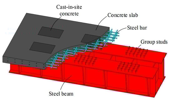
Figure 1.
Prefabricated steel–concrete composite beams.
The stress between the concrete slab and the steel beam of the composite beam is mainly transferred by the shear connection; so, it has a great influence on the deformation and stress of the composite beam. Among them, stud shear connectors are the most commonly used shear connectors with better construction technology and better bridge stress performance. Experts and scholars have conducted rich research on stud connectors and obtained fruitful results. From the research methods, the study of interface performance can be divided into three kinds: experimental studies, theoretical models, and numerical analysis. In terms of experimental research, the force–displacement relationship is the most important mechanical performance of the stud connector and includes the longitudinal shear–slip relationship and the vertical upward pulling force–lift displacement relationship, which are generally obtained by push-out and pull-out tests, respectively. The shear–slip formula proposed by Ollgard et al. [1] is widely used and has been introduced into the European code 4 [2]. The formula specifies the shear bearing capacity of the composite beam studs as the smaller part of the strength of the studs themselves and the local compressive capacity of the surrounding concrete. The pull-out test shows that the pull-out capacity of the composite beam stud is also smaller than the ultimate tensile capacity of the stud’s parent material and the damage capacity of the surrounding concrete cone. For the theoretical model research, due to the deformation of the shear connectors, there are longitudinal slips and vertical lift-off displacements at the interface. These lead to the section conversion stiffness method being unable to accurately calculate the force performance of the composite beams, and the calculation results are on the unsafe side. The researchers proposed a theoretical model for the composite beam considering the longitudinal slips and vertical lift-offs at the interface. The principle involves introducing new degrees of freedom functions based on the primary beam (Euler beam or Timoshenko beam), including the slip function (to simulate the longitudinal slip) [3], the vertical separation displacement function (to simulate the vertical lift deformation) [4], and the shear hysteresis strength function (to simulate the shear hysteresis effect) [5]. The model solutions include theoretical analytical solutions [6], finite element methods [5,7], and finite difference methods [8]. Some studies that investigated numerical models of composite beams have demonstrated the reliability and adequacy of this approach. [9,10,11,12] For numerical analysis, four methods are mainly used to simulate the force performance of the composite beam studs: (1) the use of solid elements to simulate the studs [13], which can finely simulate the local force state of the studs and the surrounding concrete and is mostly used in the fine analysis of the local range of the composite beam interface; (2) the use of beam elements to simulate the studs, which can simplify the computational scale of the finite element model to the greatest extent and is mostly used in the numerical calculation of the overall force performance of the composite beam; (3) the simulation of the studs by spring elements [14,15], with the elements adopting a force–displacement macroscopic constitutive model instead of the stress–strain microscopic constitutive model; and (4) the simulation of the studs by setting the face-to-face contact relationship [16], which is only applicable to the case of homogeneous studs. A large number of studies have been performed on the force performance of the composite beam interface. These studies are basically carried out by focusing on the acquisition or application of the force–displacement macroscopic intrinsic relationship of the studs.
Group stud connectors are the most important structure for prefabricated composite beams to ensure that the steel beam and concrete slab work together. Xu et al. [17,18,19,20] analyzed the shear resistance and damage process of the group studs by means of push-out tests and finite element simulations. Then, Xu et al. investigated the effect of the concrete cracks caused by bending moments on the push-out tests of cluster studs. The pull-out performance of group studs has been little studied. Huang et al. [21] conducted pull-out tests on group studs and found that the average ultimate pull-out capacity of the group studs was discounted to a certain extent compared to the ultimate pull-out capacity of individual studs. The conclusion from the above study is that the mechanical performance of a stud in group studs is reduced compared with the uniform arrangement. In addition, the group studs effect is not only influenced by the number of studs, rows, and concrete strength but is also related to the loading method, loading process, loading magnitude, stud stressing state, and shear connection degree.
The coupling analysis and solution of the train–track–bridge system is an important reference for judging the working performance of railroad bridges, which is a very important part of their dynamic analysis. Diana and Cheli [22] studied the dynamic interaction of the train–bridge system comprehensively and systematically by considering the track contact and the elasticity of the track. Then, they established a finite element model of the train–track–bridge dynamic interaction. Their finite element model of the train–track–bridge dynamic interaction for different types of bridges and track structures was established and validated, and the model results were in good agreement. Lv [23] combined the finite element software ANSYS with the multibody dynamics software UM to analyze the train–track–bridge refined finite element model based on the stiffness degradation method and creatively introduced the bridge damage state. Finally, from the level of bridge health monitoring, an assessment method for the condition of high-speed railway bridges during operation was proposed. To obtain as accurate a dynamic response as possible, the train–track-bridge dynamics model needs to be analyzed in a more refined way. Refined modeling based on large finite element analysis software can perform more detailed parametric analysis, which can save a lot of energy.
Much of the current study of damage to composite beams has focused on static damage from destructive moment and shear. Study on the damage caused by vibration is relatively lacking. The effect of connection damage on the overall structure has been widely investigated. However, less attention has been paid to the detailed effect of damage to the mechanical performance of the interface connection, which is important. The dynamic analysis of train–track–composite beam coupling systems with damage has mostly focused on the effects caused by the stiffness degradation of the overall structure. The effects caused by local damage have been neglected. As the dynamic damage at the interface of the composite beam and its effect on the connection and working performance of the composite beam are still unclear, this study intends to carry out a three-part research work through numerical simulation. The first is to establish an elaborate finite element model of the steel–concrete composite beam to study the dynamic response of the composite beam under a high-frequency impact load. Then, based on the elaborate composite beam model, the local specimen model with damage is obtained after cutting. Numerical simulations of push-out and pull-out tests are performed to obtain the force–displacement macroscopic constitutive relationship between the damaged and the undamaged group stud connectors. Based on the obtained macroscopic intrinsic structure relationship, a finite element model of the coupled train–track–composite beam coupling system is established to study the dynamic response of the damaged and undamaged composite beam when the train passes. As a result, the concrete slab damage and stud connection degradation of the composite beam under a high-frequency impact load and their effects on the working performance of the composite beam are obtained.
2. Elaborate FEM of the Prefabricated Steel–Concrete Composite Beam
2.1. The Generation of FEM
In this study, a combined steel–concrete beam was designed with the dimensions shown in Figure 2. The steel beam and the concrete slab are connected by group studs. The entire beam has 12 studs at each end, arranged in 3 rows of 4 studs each, with a transverse and longitudinal spacing of 400 mm. The studs have a rod diameter of 22 mm and a height of 230 mm and a stud head diameter of 35 mm and a height of 10 mm. The rest of the interface is unconstrained. The restraint conditions for the simply supported beam are set for both the left and right sides, as shown in Figure 2a.
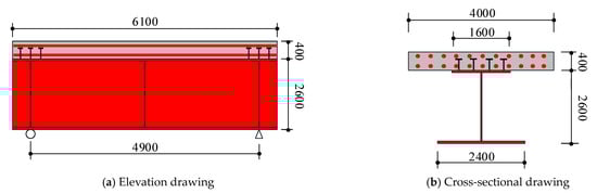
Figure 2.
Elevation and cross-section diagrams of the composite beams (unit: mm).
In this study, a finite element model of the designed combined beam was established based on the large finite element platform ABAQUS. As shown in Figure 3, there are five major components in the finite element model of the composite beam: the concrete slab, the steel beam, the studs, the reinforcement, and the loading board. To finely analyze the performance of the concrete slab and the studs, the concrete, steel beam, and stud connections are modeled by solid (C3D8R) cells; the steel reinforcement is modeled by truss (truss) cells; and the loading plate is modeled by solid (C3D8R) cells. As the difference between the size of the studs and the model of the combined beam is too large, on the basis of global meshing, a more refined meshing should be used for the studs and the stress-concentrated areas, such as the intersection of the concrete and steel beams where the studs are in contact with each other, as shown in Figure 4. The steel beam was meshed by an automatic meshing tool in ABAQUS with a mesh size of 100 mm. Figure 4a shows the element meshing of the concrete slab. In order to match the stud profile, the element sizes of the concrete slab from top to bottom in the vertical direction are 80 mm, 80 mm, 10 mm, 115 mm, and 115 mm. The element meshing of studs is shown in Figure 4b.
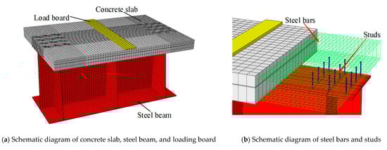
Figure 3.
Elaborate FEM of the steel–concrete composite beam.
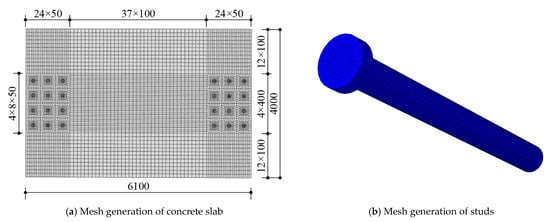
Figure 4.
Elaborate mesh generation of the critical parts.
The frictional effect between the steel beam and the concrete is ignored in this modeling process, i.e., the face-to-face contact modes of tangential frictionless (Frictionless) and normal hard contact (Hard Contact) are adopted between the steel beam and the concrete. The tangential friction between the studs and the concrete contact surface is simulated by the penalty friction, and the tangential friction coefficient is 0.4. The normal pressure transfer is simulated by hard contact. The bottoms of the studs are bound to the steel beam. The reinforcement is simulated by embedding in the contact module, the reinforcement element is embedded into the concrete element, and the bond slip between them is ignored. The loading plate is set as a rigid body and is bound to the top surface of the concrete.
2.2. Material Properties of FEM
2.2.1. The Constitutive Relation of Concrete
To better simulate the mechanical behavior of the concrete, the plastic damage intrinsic model of concrete from the ABAQUS material database was used in this study. The model uses damage factors dc and dt to characterize the degradation of the concrete material stiffness, where, when d = 0, the stiffness of the concrete material is not degraded and is within the elastic phase; when d = 1, the stiffness of the concrete material undergoes complete degradation, and the unloaded elastic mode is zero.
According to the relevant provisions of the Code for the design of concrete structures (GB50010-2010) [24], the expressions of the uniaxial compressive principal structure relationship for concrete materials are shown in Equations (1)–(5):
where αc is the parameter value of the falling section in the uniaxial compressive principal relationship curve of the concrete material, taken as 2.48; fc,r is the representative value of the uniaxial compressive strength of the concrete, taken as 38 MPa; εc,r is the peak compressive strain of the concrete corresponding to fc,r, taken as 0.00176; Ec is the elastic modulus of the concrete material, taken as 34,500 MPa; and dc is the damage factor of the concrete under compression.
The expressions for the uniaxial tensile principal structure relationship for concrete materials are shown in Equations (6)–(9):
where αt is the parameter value of the falling section in the uniaxial tensile principal relationship curve of the concrete material, which is taken as 2.17; ft,r is the representative value of the uniaxial tensile strength of the concrete, which is taken as 2.64 MPa; εt,r is the peak tensile strain of the concrete corresponding to ft,r, which is taken as 0.00011; Ec is the modulus of elasticity of the concrete material, which is taken as 34,500 MPa; and dt is the tensile damage factor of the concrete.
Based on the theories listed above, the principal structure relationship curves of the C50 concrete used in this paper are shown in Figure 5.
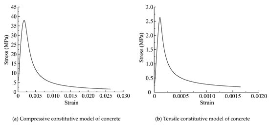
Figure 5.
Stress–strain curve of C50 concrete.
The value of the damage factor d used in this paper is shown in Figure 6.
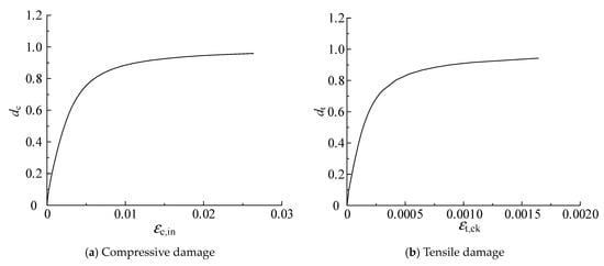
Figure 6.
Plastic damage factor of concrete.
The detailed values of the remaining parameters in the plastic damage principal structure model for concrete materials are shown in Table 1.

Table 1.
Parameters of the plastic damage constitutive model of concrete.
2.2.2. The Constitutive Relation of Steel
The materials of both the steel beam and the reinforcement are defined using ideal elastoplastic models, and the materials of the pins are defined using a bilinear model, as shown in Figure 7.
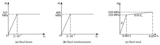
Figure 7.
Stress–strain curve of the steel.
To better simulate the influence of the stress state at which the stud is loaded on its cracking strain, a plastic damage intrinsic model of the stud is introduced in this paper, and the relationship between the triaxial stress and the cracking strain of the stud material is shown in Equation (10) [25]:
where PR is the equivalent metal cracking strain; εR is the cracking strain of the metal under uniaxial loading; ν is Poisson’s ratio of the metal material (taken as 0.3); σm is the average stress; σeq is the equivalent Mises stress; and S0 is a constant factor, taken as 1.5.
The spatial cracking strain of the metal is usually replaced using the equivalent cracking strain of the metal according to Equation (10). The plastic damage intrinsic relationship curve of the stud is shown in Figure 8. In this model, there is an exponential relationship between the equivalent plastic displacement and the damage factor d. According to the mesh refinement of the stud in the finite element model, the exponential factor between them is taken as 0.01 in this paper.
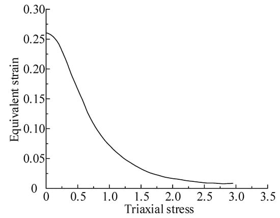
Figure 8.
Plastic damage model of the studs.
2.3. Rayleigh Damping Model
The damping coefficients of each member material in this paper are calculated by Rayleigh damping, as shown in Equation (11):
where α is the mass damping factor, β is the stiffness damping factor, C is the damping matrix, M is the mass matrix, and K is the stiffness matrix.
The Rayleigh damping coefficients for the finite element model of the combined beam are shown in Table 2.
Table 2.
Rayleigh damping coefficient of composite beams.
2.4. Dynamic Response of the Composite Beam
To simulate the action of two rows of wheel pairs in the bogie of a rail train, an “M” wave load is applied in the span of the combined beam model with a frequency of 6 Hz. The amplitude curve of an “M” load cycle is shown in Figure 9.
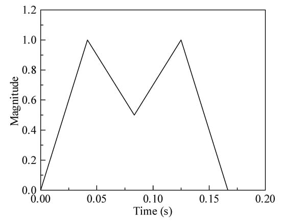
Figure 9.
Amplitude–time curve of the “M” type load.
An explicit solver with a small convergence error was used to solve the numerical model, which was proven to be accurate and reliable. Through the dynamic analysis of the finite element model of the combined beam with group studs, the respective vertical acceleration (vertical acceleration) and vertical displacement (vertical displacement) time curves of the steel beam and concrete slab of the combined beam model were obtained, as shown in Figure 10, where the positive directions of acceleration and displacement are vertically upward. In general, the acceleration and displacement time curves of the concrete slab and steel beam are significantly different. Figure 10a shows that the maximum acceleration of the concrete slab is 4.06 m/s2 and that of the steel beam is 4.61 m/s2. From the location of the local peaks of the acceleration time curves of both materials, there are certain phase differences between the two curves. Figure 10b shows that the maximum displacement of the concrete slab is 0.95 mm and the maximum displacement of the steel beam is 2.51 mm; the two displacement time curves are roughly cyclic: both displacements have the same trend in the initial stage, and the concrete slab reaches the negative displacement peak before the steel beam and then gradually decreases to the displacement zero point and then gradually increases to the positive displacement peak, while the displacement of the steel beam continues to increase after the concrete slab reaches the negative displacement peak until its negative displacement peak, and then, it gradually decreases until it is equal to the positive displacement peak. The displacement of the steel beam continues to increase after the concrete slab reaches the peak of negative displacement until it reaches the peak of negative displacement and then gradually decreases until it is equal to the displacement of the concrete slab. After that, the time course of displacement of the two beams changes approximately in the same way as this process. In this process, the concrete slab and the steel beam are separated, especially when they are in the negative displacement regime.
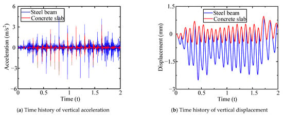
Figure 10.
Time history of acceleration and displacement of the composite beam.
3. Degradation of Mechanical Properties of Connectors Caused by Vibration Damage
3.1. FEM of Local Specimens with Vibration Damage
To analyze the performance degradation of the interface connection of the composite beam, finite element simulations of the local model of the stud arrangement area at both ends of the existing damaged composite beam were carried out to launch the pull-out tests. The model from the previous dynamic analysis was replicated to account for vibration damage, and the rest of the model was removed by the part-cutting function in ABAQUS, keeping the local model of the stud arrangement area for the subsequent push-out and pull-out tests, as shown in Figure 11. The settings of the material properties and the contact relations of the existing damaged specimen model are the same as those of the previous elaborate FEM. Based on the existing damaged specimens, the FEM of the undamaged specimens was also established to investigate the effect of the degradation of the interfacial shear connection properties. The undamaged specimen model has the same settings as the existing damaged launch specimen except that the initial state is not applied.
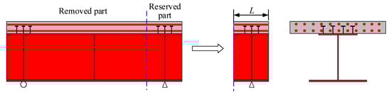
Figure 11.
Finite element model of specimens with existing damage.
In this paper, two local specimen lengths are set up for each of the two types of tests. The length of the existing damaged specimen (S-1) and the undamaged specimen (S-2) used to launch the test is L1 = 2000 mm. The length of the existing damaged specimen (S-3) and the undamaged specimen (S-4) used for the pull-out test is L2 = 1200 mm. Specimen S-1 was set up with a completely fixed restraint on the left side (cutting side) of the steel beam and concrete slab; the bottom surface of the steel beam was left with only the degree of freedom of the translational movement along the length of the beam, and the rest were all restrained; the cross-section was coupled to a reference point in the center on the right side of the steel beam, and the loading process of the roll-out test was simulated by applying a horizontal displacement load to the reference point. The bottom surface of the concrete slab of specimen S-3 was set with a completely fixed restraint; the bottom surface of the steel beam had only vertical translational degrees of freedom, and the rest were all restrained; the bottom surface of the steel beam was coupled to a reference point in the center, and the loading process of the pull-out test was simulated by applying a vertical displacement load to the reference point. The boundary conditions and the loading methods of specimens S-2 and S-4 were set in the same way as S-1 and S-3, respectively.
3.2. Results of Push-out Specimens
The load–slip curves of the specimen models were obtained by the finite element analysis of S-1 and S-2, as shown in Figure 12. The curve of S-1 has basically the same trend as the curve of S-2, which also goes through the elastic, yielding, and breaking stages. The load–slip curve first grows linearly; then, the growth rate slows down until the ultimate load is reached, the curve begins to decline, and finally, the studs shear off and break. The force performance indices of S-1 and S-2 are listed in Table 3. The vibration damage of the concrete slab has an effect on the ultimate shear capacity and slip of the pinned joints, and compared with S-2, the ultimate shear capacity of S-1 decreases by 24.8%, and the ultimate slip decreases by 15%.
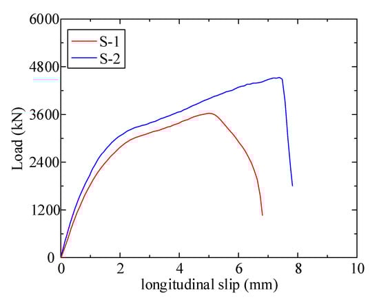
Figure 12.
Load–longitudinal slip curves of S-1 and S-2.
Table 3.
Result comparison of push-out test specimens.
With the gradual increase in the displacement load, the root of the stud first starts to yield, and the stress level basically decreases in the direction from the root to the head of the stud. When the load reaches the ultimate shear load capacity of the stud, the stress at the root of the stud reaches 430 MPa. Then, the elements at the root gradually fade away until all the elements at the bottom of the corresponding studs disappear at the limit of the slip. The Mises stress distribution in the ultimate load-carrying capacity phase for the row of studs of S-1 and S-2 is shown in Figure 13.
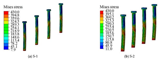
Figure 13.
Mises stress of the studs in the push-out specimens at the ultimate bearing capacity (MPa).
During the loading process, the concrete changes in the root area of the stud connector are more concentrated, and the closer the hole is to the stud connector, the greater the stress, and the damage only exists near the stud connector. During loading, the shear force is transferred from the steel beam to the stud, and the studs squeeze the concrete at the root of the stud, where the concrete has a high stress level; the stud deforms in the shear and separates from the concrete above the stud cap; so, the concrete above is subjected to less force. The damage of the concrete slab at the end of loading is shown in Figure 14, which ignored the area further away from the studs. It can be seen that the concrete at the root of the stud is more severely damaged in the tension, and the damage covers the entire vicinity of the hole; the damage in the compression mainly occurs in the area of the hole in the direction of the loading at the root of the stud. The maximum tensile stress in the concrete slab of specimen S-1 was 7.8 MPa, and the maximum compressive stress was 15.9 MPa; the maximum tensile stress in the concrete slab of S-2 was 4.1 MPa, and the maximum compressive stress was 20.8 MPa. The maximum stresses all occur in the concrete slab at the holes where the studs are located.
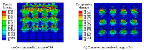
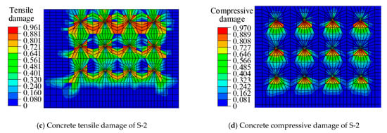
Figure 14.
Concrete damage of S-1 and S-2.
3.3. Results of Pull-out Specimens
The lift displacement curves of the specimen models were obtained by performing finite element analysis on S-3 and S-4, as shown in Figure 15. The curves of S-3 largely overlap with those of S-4, which also go through the elastic, yielding, and breaking stages. The lift displacement curve first grows linearly, and then, the growth rate slows down until the curve starts to fall after reaching the ultimate load. There is an obvious step in the descending section because the individual studs with higher stresses are the first to break; the tension is redistributed in the remaining studs, and eventually, the remaining studs are also pulled off and lose their load-carrying capacity. There is an obvious step in the descending section because the individual studs with higher stresses are damaged first, and the tensile force is redistributed in the remaining studs. Finally, the remaining studs are also pulled off and lose their bearing capacity. The force performance indices of S-3 and S-4 are listed in Table 4, which shows that the previous vibration damage has little effect on the tensile load capacity of the studs.
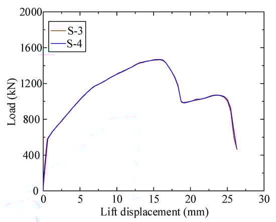
Figure 15.
Load–lift displacement curves of S-3 and S-4.
Table 4.
Result comparison of the pull-out test specimens.
The numerical simulation shows that the Mises stress of the studs in S-3 and S-4 is almost the same. The Mises stress distribution of the S-3 specimen studs during the significant loading phase is shown in Figure 16. At the initial loading, most of the stud stresses were concentrated in the range of 10–60 MPa, with the maximum stress of 107 MPa appearing at the middle row of studs; with the gradual increase in the displacement load, the root of the stud first began to yield, and the stress level basically decreased gradually in the direction from the root of the stud to the head. When the load reached one-half of the ultimate pull-out capacity of the studs, the maximum stress of the stud reached 350.6 MPa, which appeared at the root of the stud and the middle row of studs; when the load reached the ultimate pull-out capacity of the stud, the stress at the root of the stud reached 430 MPa, and the necking phenomenon appeared at the root of the middle row of studs. When the displacement load continues to increase, the middle row of studs will be damaged first, and the studs on both sides will also start to show the necking phenomenon; the displacement load is continually increased until the studs on both sides are all pulled off and damaged, at which time the elements at the studs that were pulled off and damaged all fade away. The stud stress development in specimen S-4 is also almost the same as that in S-3.
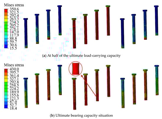
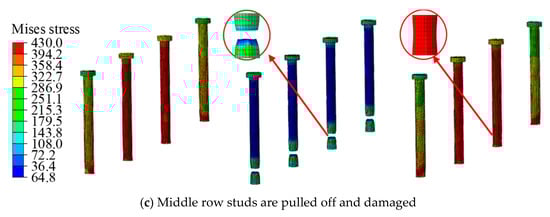
Figure 16.
Mises stress of the studs in S-3 (MPa).
The stress variation and damage to the concrete area of the hole in the stud is more concentrated. During the loading process, the tensile force is transferred from the steel beam to the studs, which deform in a tensile manner and squeeze the concrete at the bottom of the stud cap, where the concrete is under pressure, while the concrete above the stud cap is under a certain tensile force. The loading was finished, and the damage of S-3 and S-4 is shown in Figure 17, which ignored the area further away from studs. It can be seen in the figure that the concrete at the holes of the stud connectors suffered some tensile damage, while the compressive damage was not significant. The maximum tensile stress of the S-3 concrete slab was 7.6 MPa, and the maximum compressive stress was 12.7 MPa; the maximum tensile stress of the S-4 concrete slab was 8.6 MPa, and the maximum compressive stress was 12.0 MPa. The maximum stresses mentioned above are found in the concrete slab at the holes where the studs are located.
Figure 17.
Concrete damage of S-3 and S-4.
4. Effect of Connector Damage on Train–Track–Composite Beam Coupled System
In this paper, the finite element model of the dynamic interaction of a high-speed train ballastless track–composite beam bridge is established by ABAQUS, and the macroscopic constitutive models of the local specimens S-1~S-4 obtained in a previous paper are introduced (Figure 12 and Figure 15). The influence of the interface connection degradation on the overall dynamic response of the train–rail–beam system is analyzed in the case of driving a single train and crossing two trains.
4.1. FEM of High-Speed Train Ballastless Track–Composite Beam System
Based on the Code for the design of steel and concrete composite bridges (GB 50917-2013) [26] and the Code for the design of a high-speed railway (TB10621-2014) [27], a typical 40 m span simply supported by a steel–concrete composite box girder was designed. The track structure on the beam adopts the China Railway Track System II (CRTS II) ballastless track, which is widely used in China. The dimensions of the designed composite beam and track structure are shown in Figure 18.
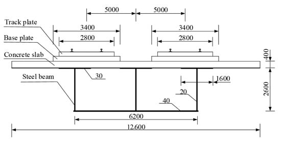
Figure 18.
Cross-section diagram of composite beam with CRTS Ⅱ ballastless track (mm).
The finite element model of the composite beam bridge is established by ABAQUS. The concrete slab adopts the solid (C3D8R) element, the steel beam adopts the shell (C43R) element, the steel bar adopts the truss element, and the stud adopts the connector element. Among them, the stiffness of the connector element of the composite beam bridge under the existing damage state is taken from the shear stiffness and the anti-lifting stiffness in the force–displacement macroscopic constitutive relationship of S-1 and S-3. The stiffness of the connector element of the composite beam bridge in the undamaged state is taken from the shear stiffness and the anti-lifting stiffness in the force–displacement macroscopic constitutive model of S-2 and S-4.
The Rayleigh damping coefficient of the composite beam bridge model is shown in Table 5, and the remaining material parameters are the same as those in Section 2.2.
Table 5.
Rayleigh damping coefficient of the composite beam with track.
We refer to the Code for the design of railway continuous welded rail (TB10015-2013) [28] and use a standard 60 kg·m−1 track, adopting a 1.435 m gauge and a 0.6 m fastener spacing. The track, track slab, and ground slab are modeled by solid elements (C3D8R). The spring-damper element is used to simulate the track and fastener. The lateral, vertical, and longitudinal equivalent stiffnesses of the fastener are 50, 35, and 15.12 MN·m−1, respectively, and the lateral, vertical, and longitudinal damping coefficients are 30, 37.5, and 30 kN·s·m−1, respectively. In the track system, except for the fastener system, the track slab and floor adopt the linear elastic constitutive model. The detailed parameters of each material are taken from TB10621-2014 [27]. In addition, the binding constraint between the base plate and the concrete slab ignores the relative displacement between them.
In the train–rail–bridge dynamic analysis, the following assumptions are made for the train model: (1) without considering the elastic deformation and relative motion of the train body, bogie frame, and wheelset in the vibration process, the train body is regarded as a rigid body with a uniform mass and as transversely and longitudinally symmetric; (2) the vibration of the carriage, bogie frame, and wheelset along the longitudinal axis are not considered; (3) the primary suspension device is mainly composed of a spring damping device between the car body and the bogie frame; (4) the secondary suspension device is mainly composed of a spring damping device between the bogie frame and the wheelset; (5) the car body contains six degrees of freedom, which are three-dimensional translational and rotational degrees of freedom; (6) when the train is running, it only performs uniform linear motion, and the longitudinal force and lateral force caused by acceleration, deceleration, and turning are not considered. The high-speed rail train set in this paper contains only one carriage. The train body is simplified into a multi-rigid body system composed of one carriage body, two bogies, and four wheelsets. The FEM is established in ABAQUS with reference to CRH2 EMU. The main parameters of CRH2 are shown in Table 6. In the model, the train compartment is simulated by a discrete rigid body, and the bogie and wheelset are simulated by an analytical rigid body. The reference points are set at the geometric center of each rigid body, in which the rigid body mass is applied by concentrated mass points, the gravity of each rigid body is applied by the equivalent loading method, and the specified concentrated force is applied at the reference points of each rigid body. The fastener element is used to simulate the primary and secondary suspension devices of the train. The specific structure of the model is shown in Figure 19.
Table 6.
Main parameters of CRH2.
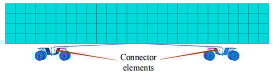
Figure 19.
FEM of single train and connector elements.
The track irregularity recommended by the German track spectrum is simulated by the inverse Fourier transform method. Using the MATLAB platform, the German low-interference track height and track irregularity samples are drawn, as shown in Figure 20. Then, the track component is divided. On this basis, the track surface coordinates are modified by the input file to realize the application of track irregularity. The details of the track model with track irregularity are shown in Figure 21.
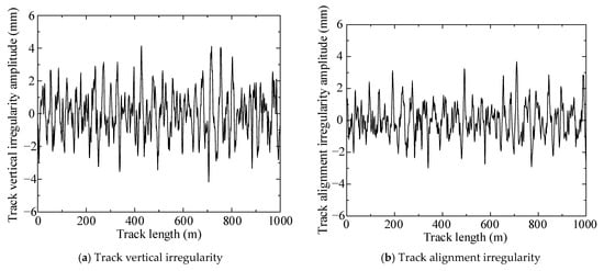
Figure 20.
Spectrum of low interference track irregularities.
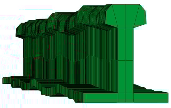
Figure 21.
Details of the track model with irregularity.
Considering the two cases of single-train driving (T-1) and the two-train intersection (T-2), the finite element models of a high-speed train ballastless track–composite beam bridge system is established based on ABAQUS. The model includes a high-speed train, a CRTS II slab ballastless track structure and a composite beam bridge. The train–rail–bridge model under single-train driving and two trains meeting is shown in Figure 22. In order to completely simulate the movement of the trains on a composite beam, the rails were extended beyond the composite beam. The tracks beyond the composite beams are fixed at the bottom.
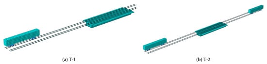
Figure 22.
Train–track–composite beam under the 2 driving conditions.
4.2. The Responses of the Composite Beams with Train Passing
To facilitate the analysis of the influence of the stud performance degradation on the overall dynamic performance of the composite beams, this paper considers three train speeds: 360 km/h, 330 km/h, and 300 km/h. The response of the composite beam bridges under the T-1 and T-2 conditions is obtained by ABAQUS dynamic analysis. The vertical displacement and lateral displacement of the composite beam span are mainly studied. According to the calculation, the times for a single train to cross the bridge are approximately 0.404 s, 0.441 s, and 0.485 s. According to the size of the finite element model, the analysis step time of the train–rail–bridge model is determined to be 1.5 s.
4.2.1. Responses of T-1
The time history curves of the mid-span nodes of the composite girder bridge under the condition of each train speed are shown in Figure 23, Figure 24 and Figure 25. The peak mid-span displacement of the composite girder bridge at the three speeds is shown in Table 7. In the case of a speed of 360 km/h, compared with the dynamic response peak of the composite beam bridge under the undamaged state, the vertical displacement peak of the composite beam bridge under the existing damage state increased by 13%, and the lateral displacement peak increased by 24.2%. In the case of a speed of 330 km/h, compared with the dynamic response peak of the composite beam bridge under the undamaged state, the vertical displacement peak of the composite beam bridge under the existing damage state increased by 8.38%, and the lateral displacement peak increased by 15%. In the case of a speed of 300 km/h, compared with the dynamic response peak of the composite beam bridge under the undamaged state, the vertical displacement peak of the composite beam bridge under the existing damage state increased by 6.2%, and the lateral displacement peak increased by 9.2%. For T-1, compared with the undamaged composite beam, the vertical displacement and lateral displacement peaks of the composite beam in the existing damage state increased by varying degrees, and the degradation of the stud performance had a greater impact on the composite beam bridges with a higher traffic speed.
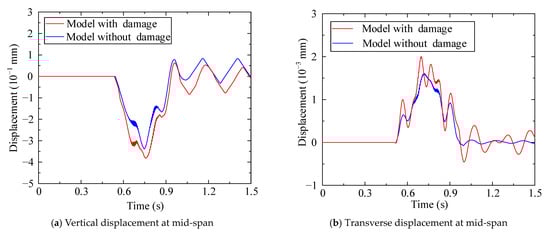
Figure 23.
Responses of the composite beam at a train speed of 360 km/h in the case of T-1.
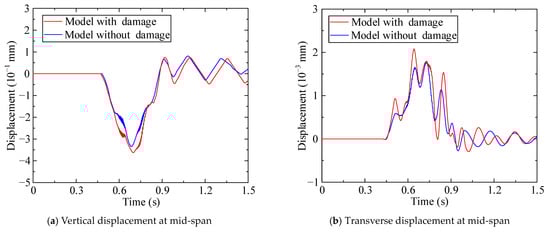
Figure 24.
Responses of the composite beam at a train speed of 330 km/h in the case of T-1.
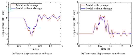
Figure 25.
Responses of the composite beam at a train speed of 300 km/h in the case of T-1.
Table 7.
Comparison of maximum displacement at mid-span of composite beams.
4.2.2. Responses of T-2
The time history curves of the mid-span nodes of the composite girder bridge under the condition of each train speed are shown in Figure 26, Figure 27 and Figure 28. The peak mid-span displacement of the composite girder bridge at three speeds is shown in Table 8. In the case of a speed of 360 km/h, compared with the dynamic response peak of the composite beam bridge in the undamaged state, the vertical displacement peak of the composite beam bridge under the existing damage state increased by 8.8%, and the lateral displacement peak increased by 26.4%. In the case of a speed of 330 km/h, compared with the dynamic response peak of the composite beam bridge in the undamaged state, the vertical displacement peak of the composite beam bridge under the existing damage state increased by 13.7%, and the lateral displacement peak increased by 53%. In the case of a speed of 300 km/h, compared with the dynamic response peak of the composite beam bridge in the undamaged state, the vertical displacement peak of the composite beam bridge under the existing damage state increased by 12.8%, and the lateral displacement peak increased by 24.8%. For T-2, compared with the composite girder bridge with traffic speeds of 360 km/h and 300 km/h, the degradation of the stud force performance had the greatest impact on the composite girder bridge with a traffic speed of 330 km/h.
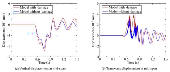
Figure 26.
Responses of the composite beam at a train speed of 360 km/h in the case of T-2.
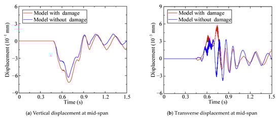
Figure 27.
Responses of the composite beam at a train speed of 330 km/h in the case of T-2.
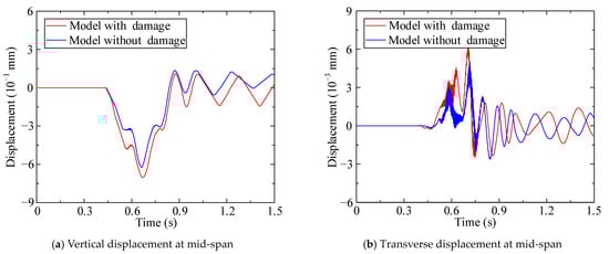
Figure 28.
Responses of the composite beam at a train speed of 300 km/h in the case of T-2.
Table 8.
Comparison of maximum displacement at mid-span of composite beams.
5. Conclusions
In this paper, an elaborate FEM of a composite beam with group studs is established based on the ABAQUS platform, and an “M” type cyclic load is applied. On this basis, the FEM of the push-out and pull-out tests of the existing damaged and undamaged local specimens was established. Then, a numerical simulation was carried out to analyze the concrete slab damage and the degradation of the connection. The coupling system of a high-speed train ballastless track–composite beam was established, in which the macroscopic constitutive model of the connection was introduced. Finally, the influence of the connection degradation on the overall behavior of the coupling system under the conditions of single-train driving and a two-train rendezvous was analyzed.
(1) For the vibration characteristics of the area without a stud constraint at the composite beam interface, there is a certain phase difference between the acceleration time curve of the concrete slab and the steel beam at the local peak of the acceleration time curve of each specimen. The displacement time curve of each specimen is basically cyclic, and the trend is that the concrete slab and the steel beam are separated at the peak of the negative displacement of the concrete slab and return to the fit state after reaching the peak of their respective positive and negative displacements.
(2) For the finite element simulation of the group stud local specimen launch, the ultimate load capacity of the existing damaged launch specimen decreased by 24.8%; the ultimate slip decreased by 15%; and the shear stiffness decreased by 12.8% compared with the force performance index of the undamaged launch specimen. In the process of conducting the finite element simulation of the group stud specimen pull-out, the studs in the middle row had higher stress and were the first to fracture, and the tensile force was redistributed among the rest of the studs, which led to an obvious step in the decreasing section of the load capacity. Compared with the stress performance indices of the undamaged extracted specimens, the ultimate load capacity of the existing damaged extracted specimens decreased by 0.2%; the lift displacement when the middle row of studs was pulled off decreased by 2.1%; the lift displacement when all the studs were pulled off decreased by 1.6%; and the pull-out stiffness decreased by 0.55%. Vibration damage had a greater effect on the shear performance of the studs and had little effect on the pull-out resistance of the studs.
(3) For the single-train travel and the two-train rendezvous, the peak vertical and lateral displacements of the existing damaged composite girder bridge increased by different degrees for different passing speeds compared to the undamaged composite girder. In the case of the single-train travel, the spanwise vertical displacements of the existing damaged composite beam increased by 13%, 8.38%, and 6.2% for the passing speeds of 360 km/h, 330 km/h, and 300 km/h, respectively, and the lateral displacements increased by 24.2%, 15%, and 9.2%, respectively, compared with the undamaged composite beam. In the case of the two-train rendezvous, the vertical displacements in the span increased by 8.8%, 13.7%, and 12.8%, respectively, and the lateral displacements increased by 26.4%, 53%, and 24.8%, respectively. In general, the degradation of the shear connection force performance during single-train travel has the greatest effect on the response of the combined girder for the 360 km/h passing speed; in the case of the two-train rendezvous, the degradation of the shear connection force performance has the greatest effect on the response of the combined girder bridge for the 330 km/h passing speed.
Author Contributions
Conceptualization, L.Z.; methodology, L.Z.; software, G.-Y.Z.; validation, G.-Y.Z.; formal analysis, J.-X.H.; investigation, G.-Y.Z.; resources, L.Z.; data curation, W.L.; writing—original draft preparation, W.L.; writing—review and editing, W.L.; visualization, J.-C.Z.; supervision, L.Z.; project administration, L.Z.; funding acquisition, L.Z. and G.-Y.Z. All authors have read and agreed to the published version of the manuscript.
Funding
The research was funded by the financial support provided by the Projects of Central Guidance for Local Science and Technology Development of China (226Z0801G) and Open Fund of National Key Laboratory of High-Speed Railway Track Technology of China (2021YJ048).
Institutional Review Board Statement
Not applicable.
Informed Consent Statement
Informed consent was obtained from all individual participants included in the study.
Data Availability Statement
The data provided in this study could be released upon reasonable request.
Acknowledgments
The authors express their thanks to the people helping with this work, and acknowledge the valuable suggestions from the peer reviewers.
Conflicts of Interest
The authors declare no conflict of interest.
References
- Ollgaard, J.G.; Slutter, R.G.; Fisher, J.W. Shear strength of stud connectors in lightweight and normal-weight concrete. AISC Eng. J. 1971, 8, 55–64. [Google Scholar]
- EN 1994-2; Eurocode 4: Design of Composite Steel and Concrete Structures, Part 2: General Rules and Rules for Bridges. European Committee for Standardization: Brussels, Belgium, 1997.
- Chakrabarti, A.; Sheikh, A.H.; Griffith, M.; Oehlers, D.J. Analysis of composite beams with longitudinal and transverse partial interactions using higher order beam theory. Int. J. Mech. Sci. 2012, 59, 115–125. [Google Scholar] [CrossRef]
- He, G.H.; Yang, X. Finite element analysis for buckling of two-layer composite beams using Reddy’s higher order beam theory. Finite Elem. Anal. Des. 2014, 83, 49–57. [Google Scholar] [CrossRef]
- Ranzi, G.; Asta, A.D.; Ragni, L.; Zona, A. A geometric nonlinear model for composite beams with partial interaction. Eng. Struct. 2010, 32, 1384–1396. [Google Scholar] [CrossRef]
- Zhu, L.; Su, R.K.L. Analytical solutions for composite beams with slip, shear-lag and time-dependent effects. Eng. Struct. 2017, 152, 559–578. [Google Scholar] [CrossRef]
- Sousa, J.B.M., Jr.; Oliveira, C.E.M.; da Siliva, A.R. Displacement-based nonlinear finite element analysis of composite beam-columns with partial interactions. J. Constr. Steel Res. 2010, 66, 772–779. [Google Scholar] [CrossRef]
- Zhu, L.; Nie, J.G.; Ji, W.Y. Positive and negative shear lag behaviors of composite twin-girder decks with varying cross-section. Sci. China Technol. Sci. 2017, 60, 116–132. [Google Scholar] [CrossRef]
- Elbelbisi, A.H.; El-Sisi, A.A.; Hassan, H.A.; Salim, H.A.; Shabaan, H.F. Parametric study on steel–concrete composite beams strengthened with post-tensioned CFRP tendons. Sustainability 2022, 14, 15792. [Google Scholar] [CrossRef]
- El-Sisi, A.; Alsharari, F.; Salim, H.; Elawadi, A. Efficient beam element model for analysis of composite beam with partial shear connectivity. Composite Structures. Compos. Struct. 2023, 303, 116262. [Google Scholar] [CrossRef]
- Alsharari, F.; El-Sisi, A.E.; Mutnbak, M.; Salim, H.; El-Zohairy, A. Effect of the progressive failure of shear connectors on the behavior of steel-reinforced concrete composite girders. Buildings 2022, 12, 596. [Google Scholar] [CrossRef]
- El-Sisi, A.A.; Hassanin, A.I.; Shabaan, H.; Elsheikh, A.I. Effect of external post-tensioning on steel-concrete composite beams with partial connection. Eng. Struct. 2021, 247, 113130. [Google Scholar] [CrossRef]
- Bonilla, J.; Bezerra, L.M.; Mirambellc, E. Resistance of stud shear connectors in composite beams using profiled steel sheeting. Eng. Struct. 2019, 187, 478–489. [Google Scholar] [CrossRef]
- Zhu, L.; Nie, J.G.; Li, F.X.; Ji, W.Y. Simplified analysis method accounting for shear-lag effect of steel-concrete composite decks. J. Constr. Steel Res. 2015, 115, 62–80. [Google Scholar] [CrossRef]
- Nie, J.G.; Pan, W.H.; Tao, M.X.; Zhu, Y.Z. Experimental and Numerical Investigations of Composite Frames with Innovative Composite Transfer Beams. ASCE J. Struct. Eng. 2017, 143, 04017041. [Google Scholar] [CrossRef]
- Guezouli, S.; Lachal, A. Numerical analysis of frictional contact effects in push-out tests. Eng. Struct. 2012, 40, 39–50. [Google Scholar] [CrossRef]
- Xu, C.; Sugiura, K.; Wu, C.; Su, Q.T. Parametrical static analysis on group studs with typical push-out tests. J. Constr. Steel Res. 2012, 72, 84–96. [Google Scholar] [CrossRef]
- Xu, C.; Sugiura, K. FEM analysis on failure development of group studs shear connector under effects of concrete strength and stud dimension. Eng. Fail. Anal. 2013, 35, 343–354. [Google Scholar] [CrossRef]
- Xu, C.; Sugiura, K. Parametric push-out analysis on group studs shear connector under effect of bending-induced concrete cracks. J. Constr. Steel Res. 2013, 89, 86–97. [Google Scholar] [CrossRef]
- Xu, C.; Sugiura, K. Analytical investigation on failure development of group studs shear connector in push-out specimen under biaxial load action. Eng. Fail. Anal. 2014, 37, 75–85. [Google Scholar] [CrossRef]
- Huang, C.P.; Zhang, Z.X.; Zheng, Z.J.; Tan, Y. Force characteristics and failure mechanism experimental study of group-nail in steel-concrete composite structure. J. Wuhan Univ. Technol. 2015, 37, 100–105. (In Chinese) [Google Scholar]
- Diana, G.; Cheli, F. Dynamic Interaction of RaiIway Systems with Large Bridges. Veh. Systen Dyn. 1989, 18, 71–106. [Google Scholar] [CrossRef]
- Lv, J. Research of Condition Assessment of High Speed Railway Bridge Based on Dynamic Interaction of the Coupled Train and Bridge. Master’s Thesis, Harbin Institute of Technology, Harbin, China, 2014. (In Chinese). [Google Scholar]
- GB 50010-2010; Ministry of Housing and Urban-Rural Development of PRC, Code for Design of Concrete Structures. China Architecture & Building Press: Beijing, China, 2010. (In Chinese)
- Lemaitre, J. A continuous damage mechanics model for ductile fracture. J. Eng. Mater. Technol. 1985, 107, 83–89. [Google Scholar] [CrossRef]
- GB 50917-2013; Ministry of Housing and Urban-Rural Development of PRC, Code for Design of Steel and Concrete Composite Bridges. China Planning Publishing House: Beijing, China, 2013. (In Chinese)
- TB10621-2014; National Railway Administration of PRC. Code for Design of High-Speed Railway. China Railway Publishing House: Beijing, China, 2014. (In Chinese)
- TB10015-2013; National Railway Administration of PRC. Code for Design of Railway Continuous Welded Rail. China Railway Publishing House: Beijing, China, 2013. (In Chinese)


Disclaimer/Publisher’s Note: The statements, opinions and data contained in all publications are solely those of the individual author(s) and contributor(s) and not of MDPI and/or the editor(s). MDPI and/or the editor(s) disclaim responsibility for any injury to people or property resulting from any ideas, methods, instructions or products referred to in the content. |
© 2023 by the authors. Licensee MDPI, Basel, Switzerland. This article is an open access article distributed under the terms and conditions of the Creative Commons Attribution (CC BY) license (https://creativecommons.org/licenses/by/4.0/).