
Response Modification Factors for Multi-Span Reinforced Concrete Bridges in Pakistan

 ,
,  , and
, and
Abstract
1. Introduction
2. Description of Reinforced Concrete Bridges
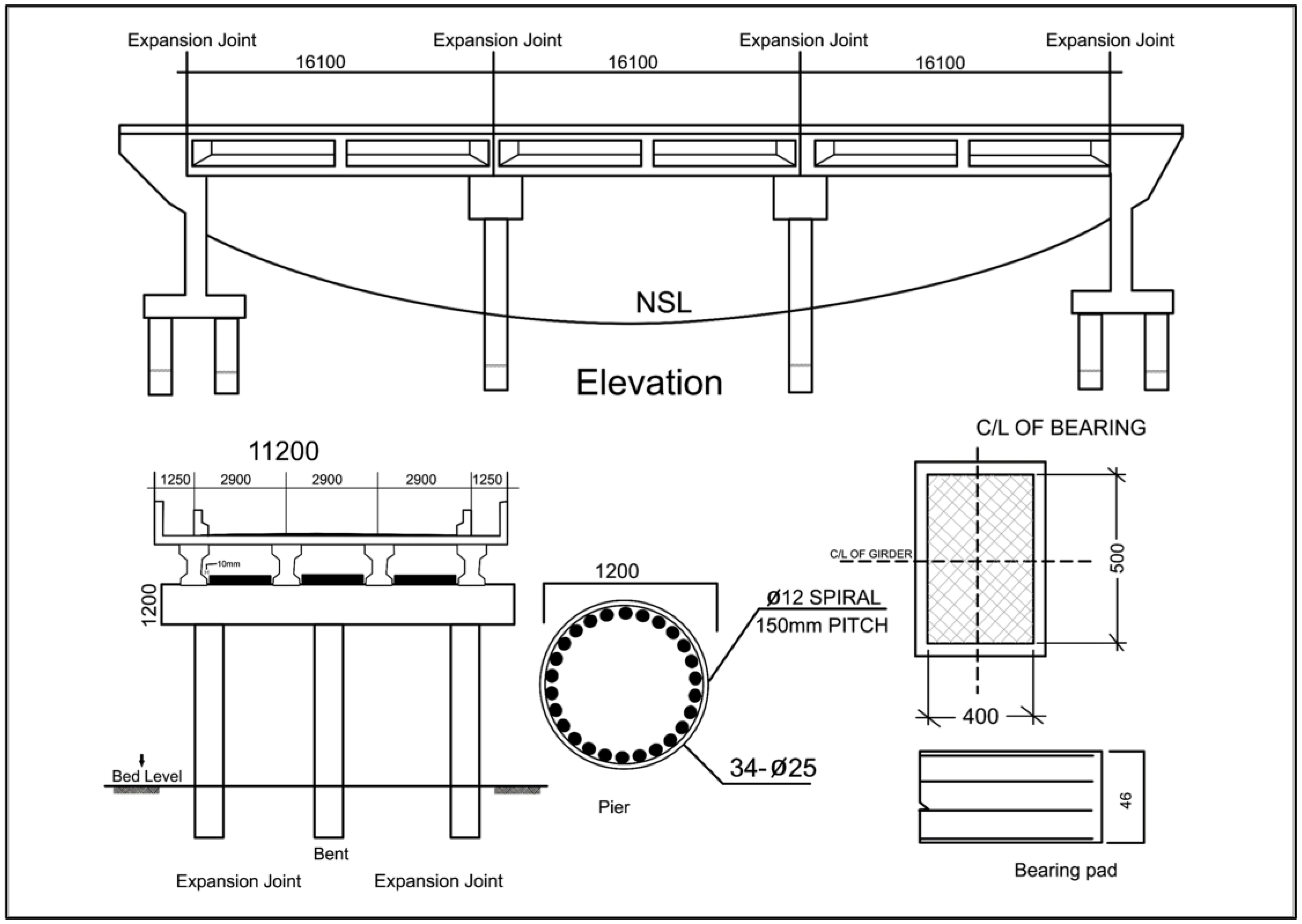
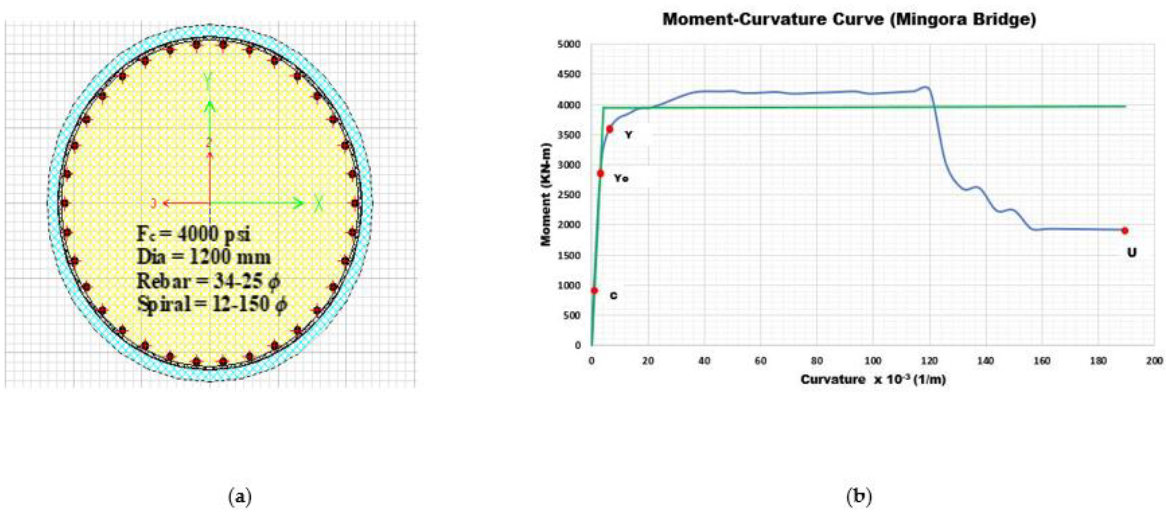
2.1. Mingora Bridge
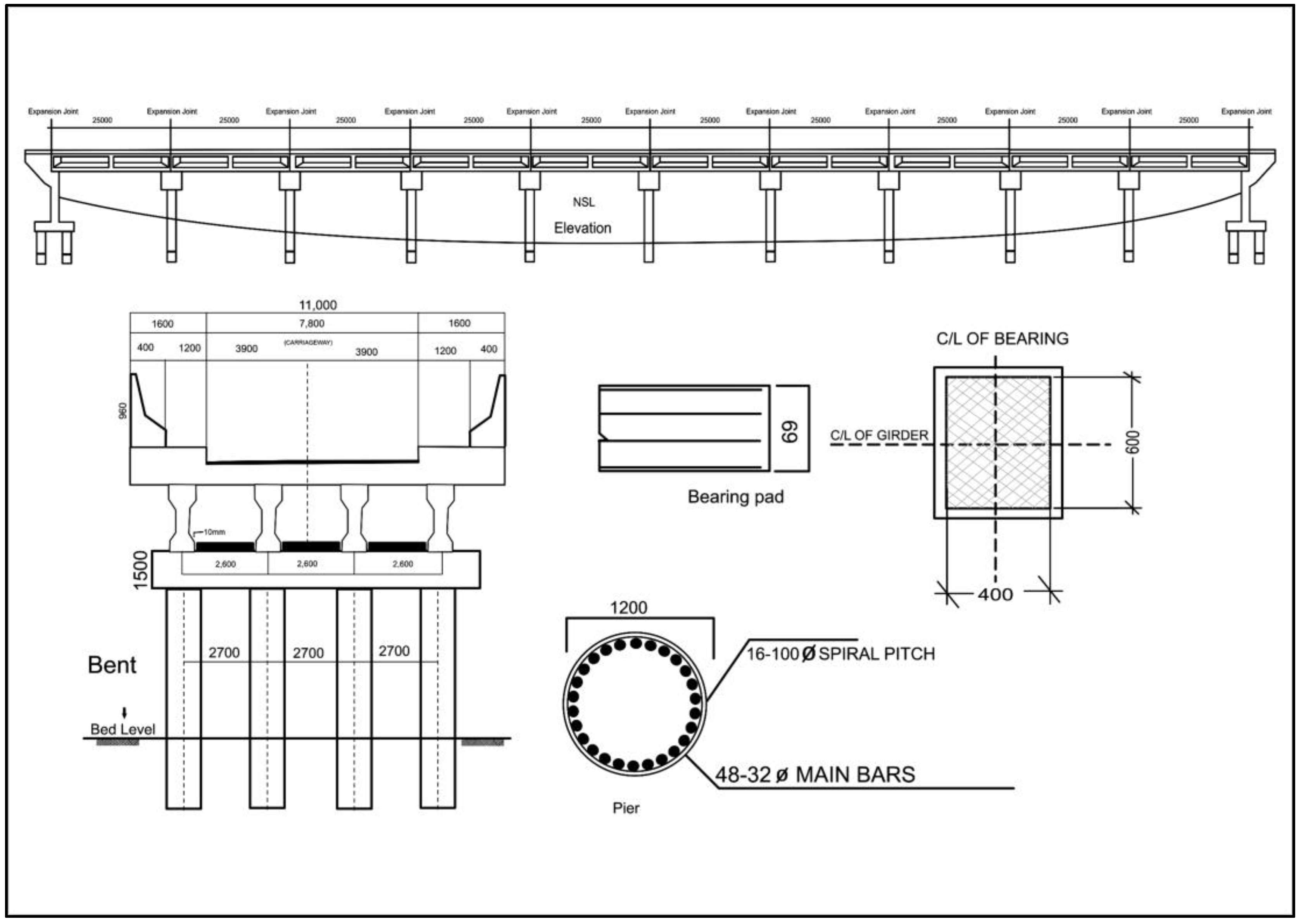
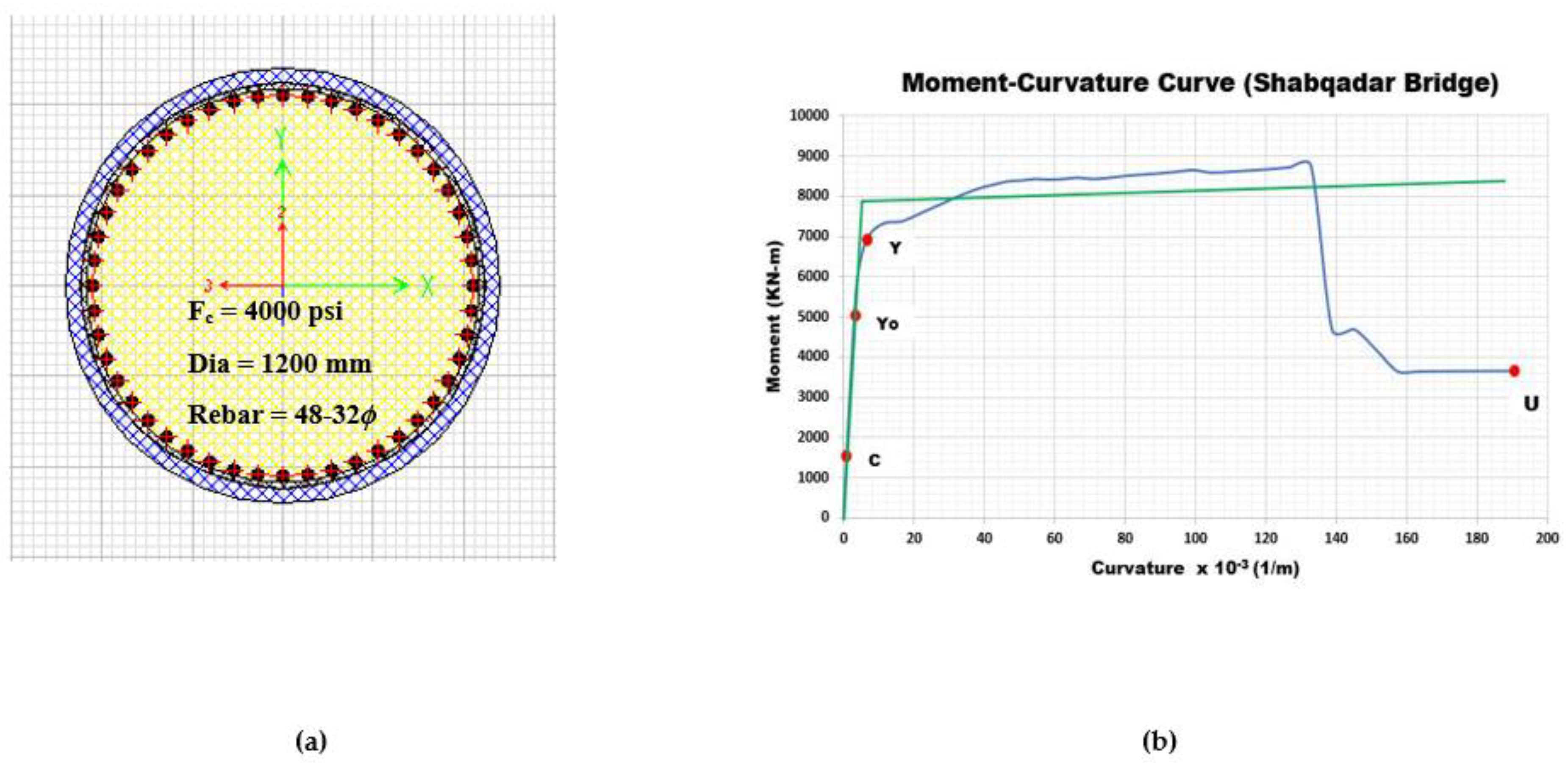
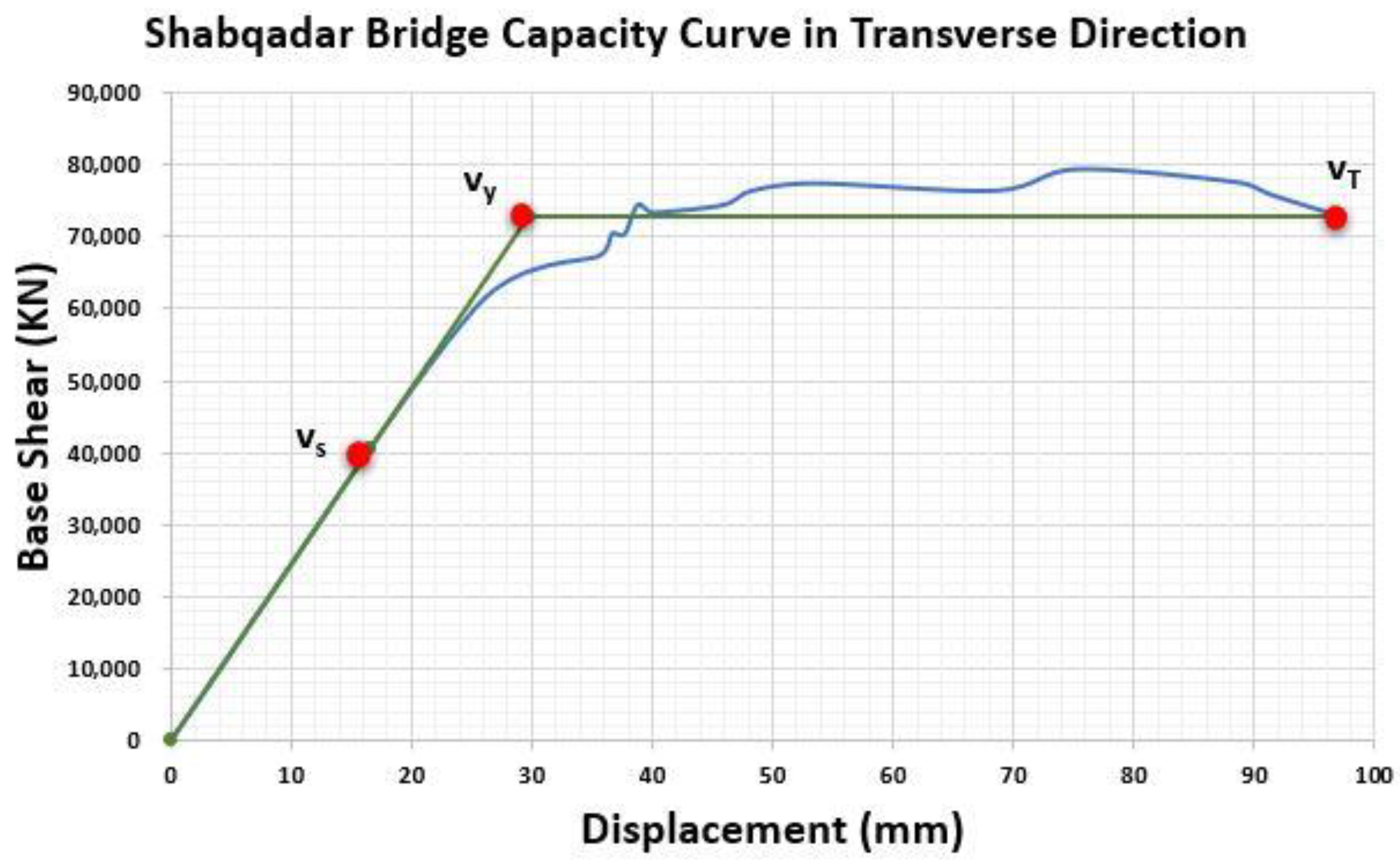
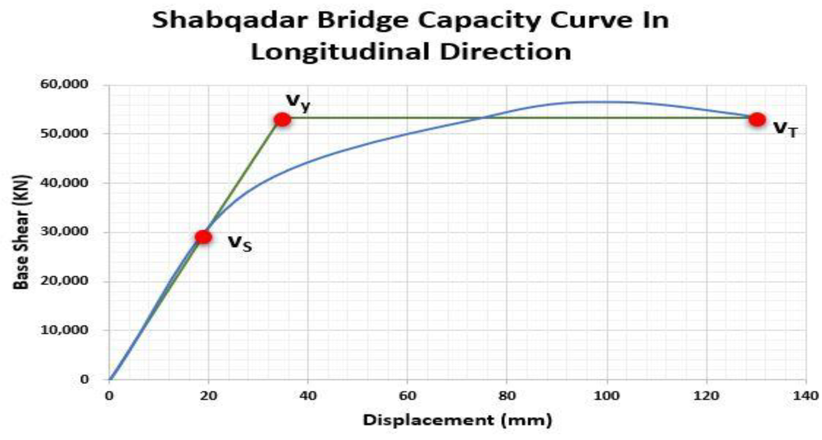
2.2. Shabqadar Bridge Charsadda
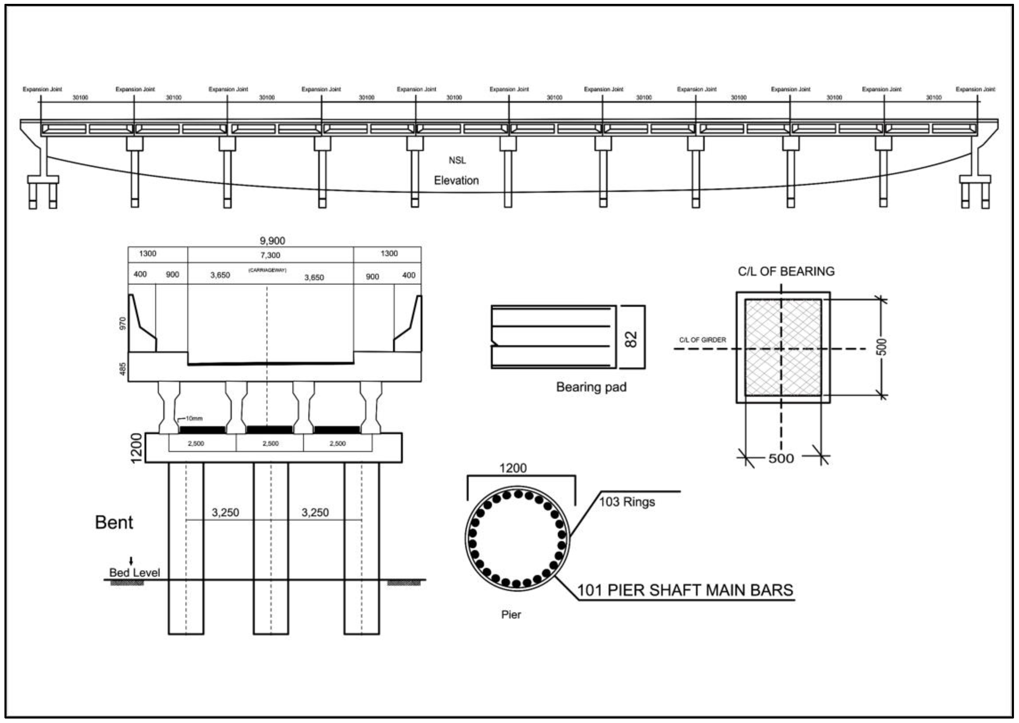
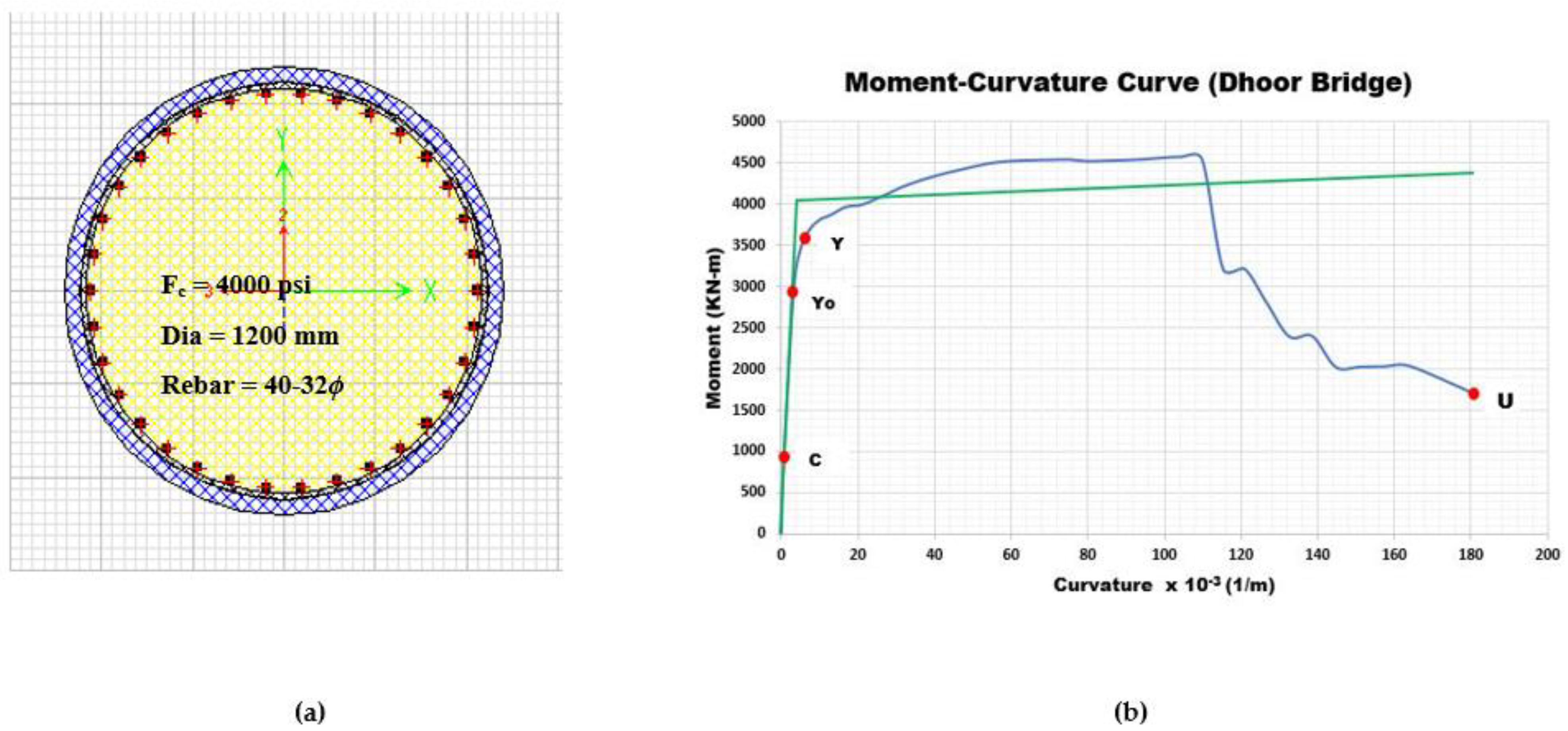
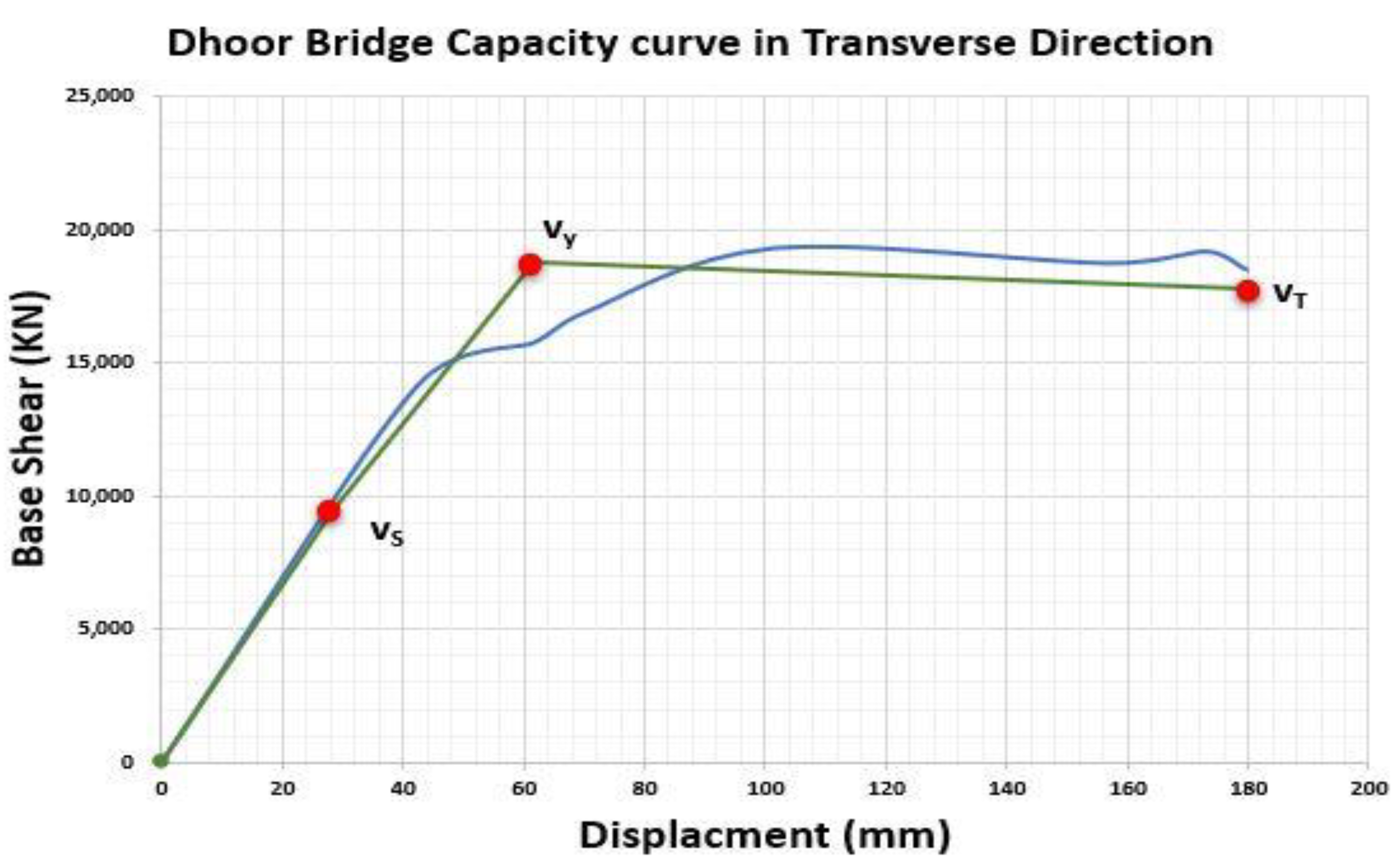
2.3. Dhoor Bridge Mansehra
3. Computational Models
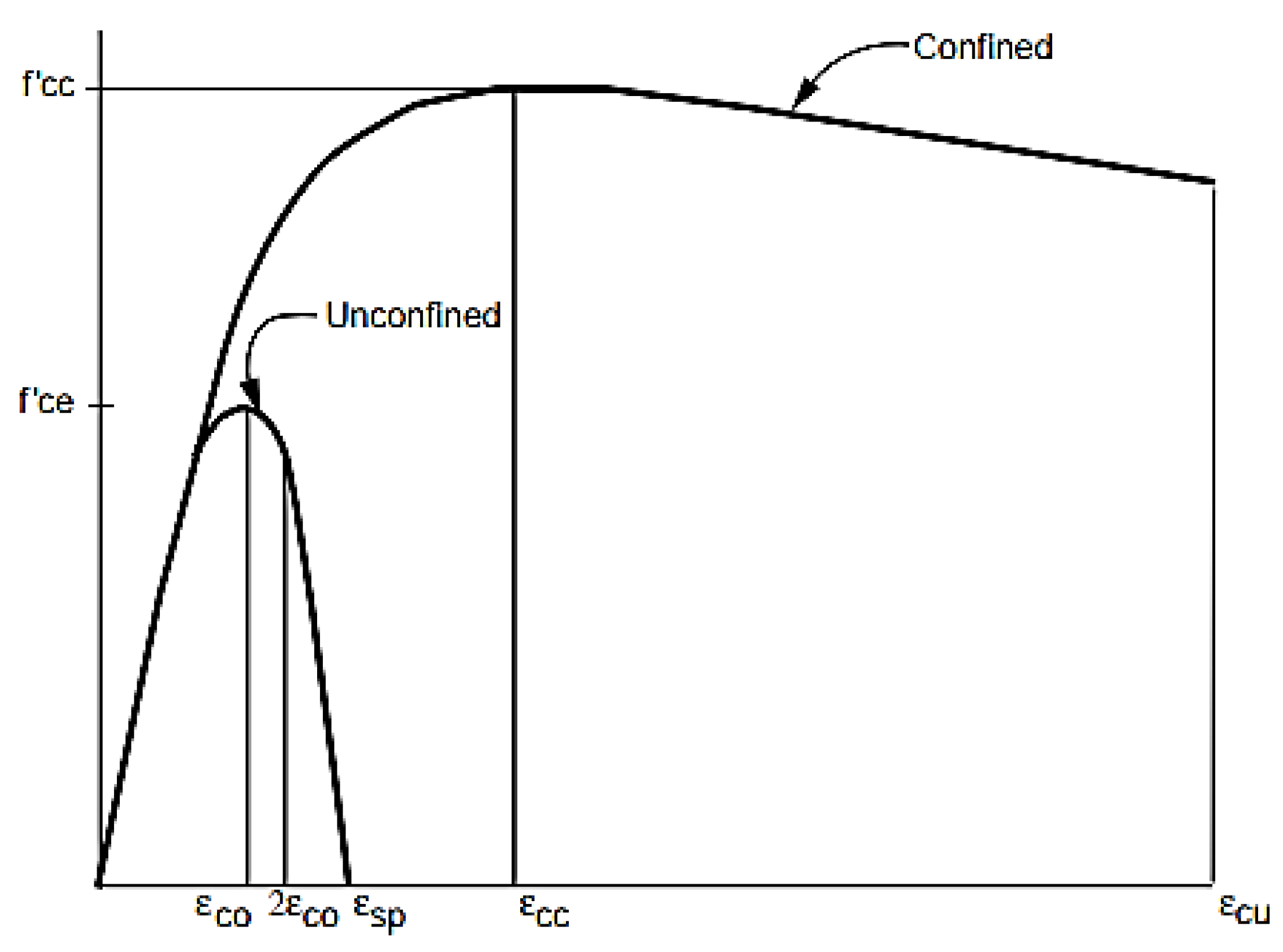
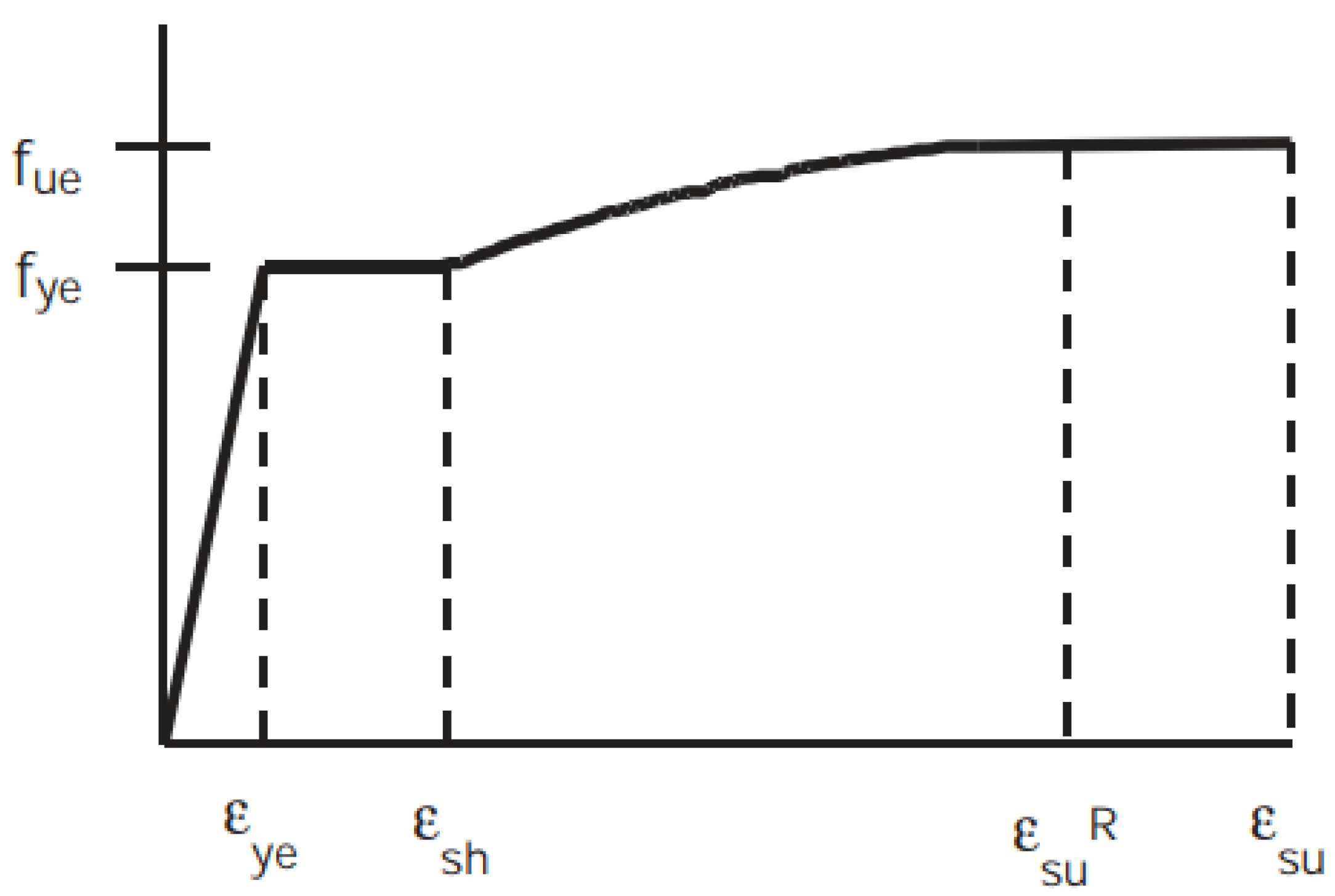
3.1. Material Properties Modeling of Bridge
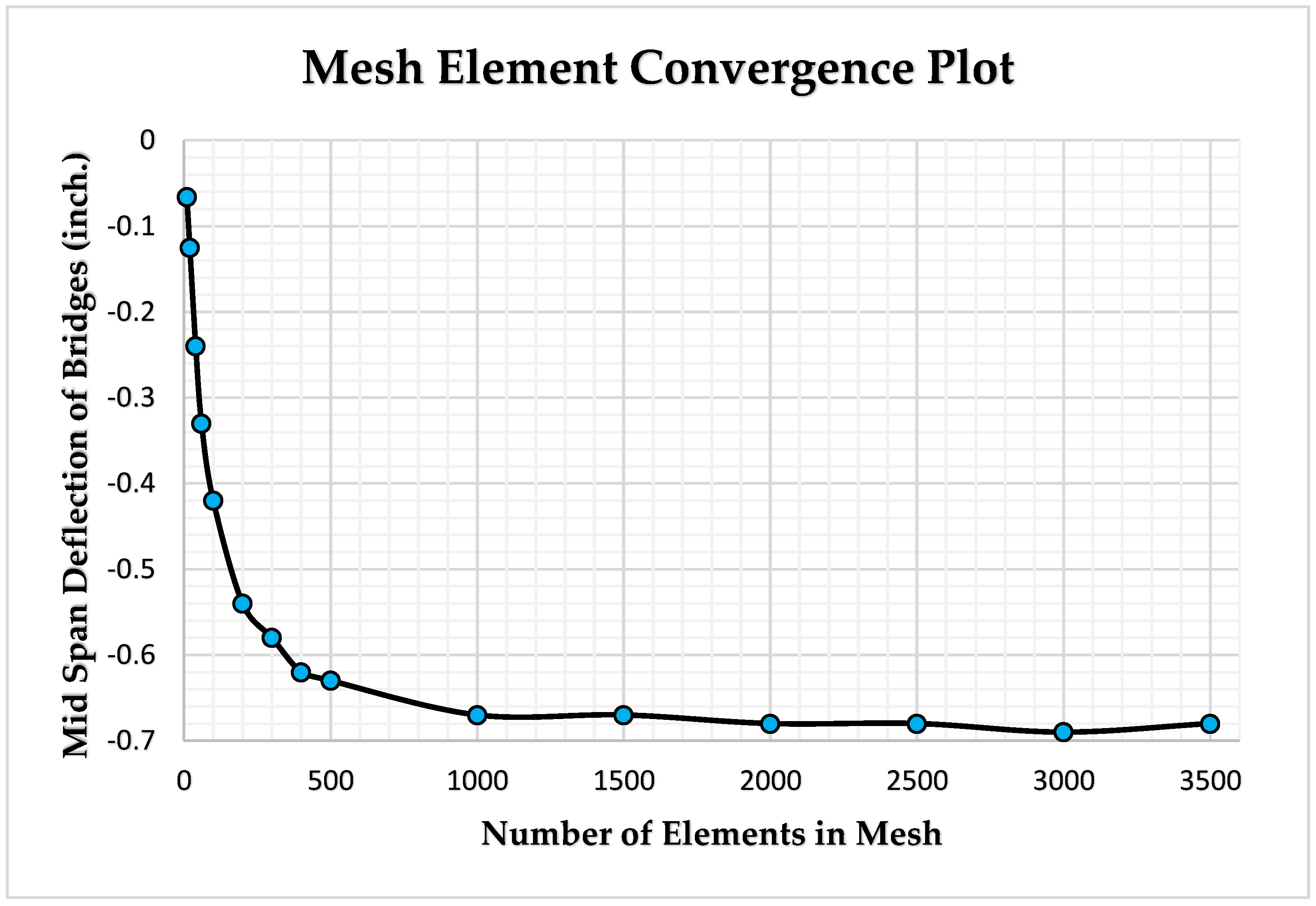
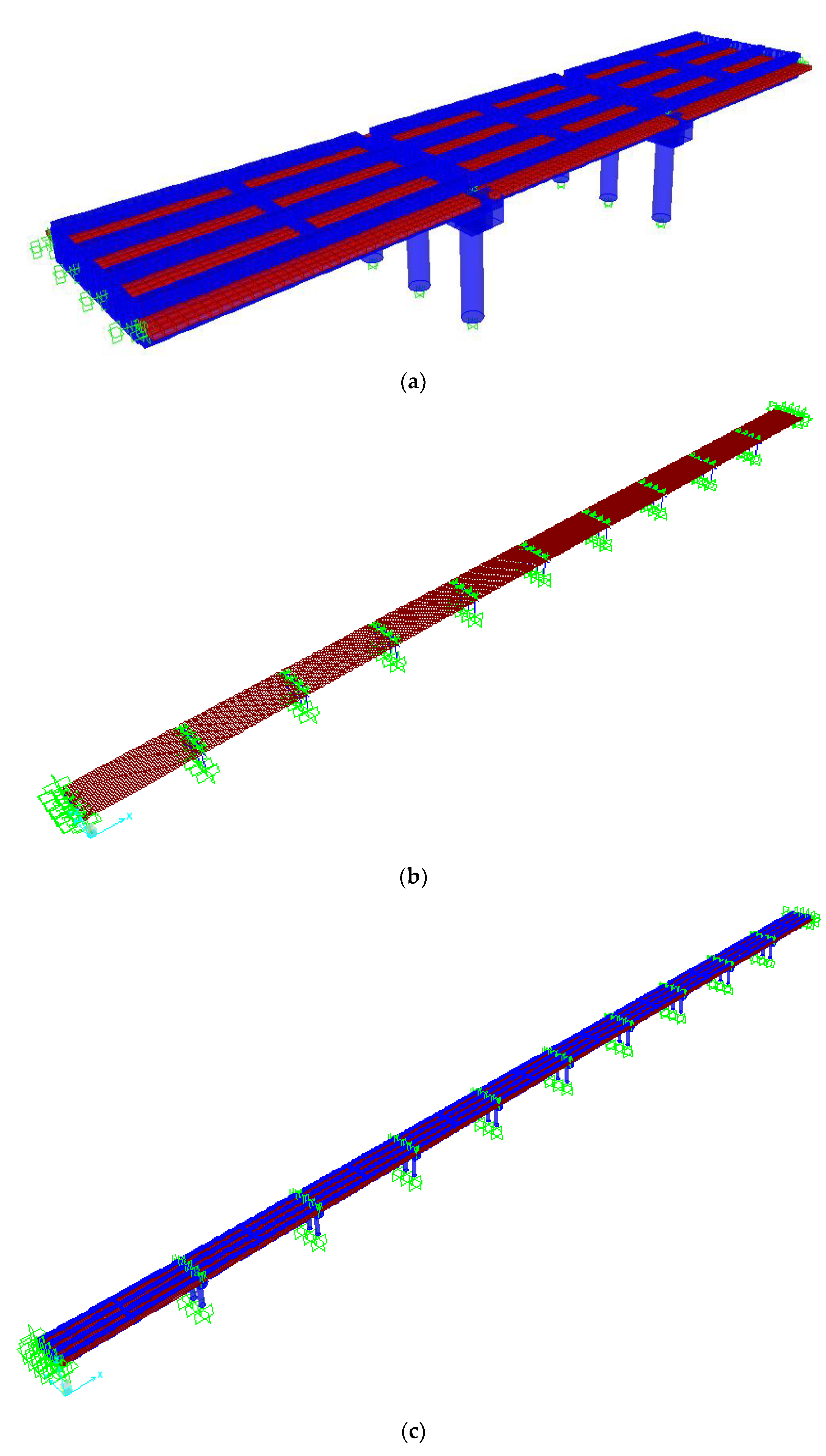
3.2. Finite Element Modeling of Bridge
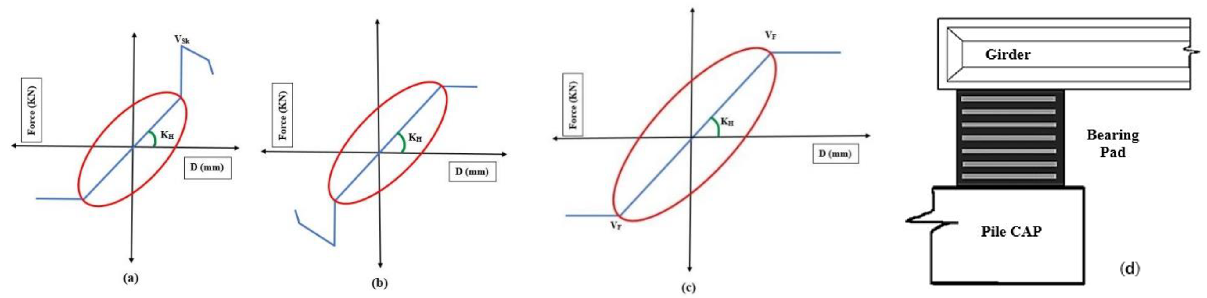
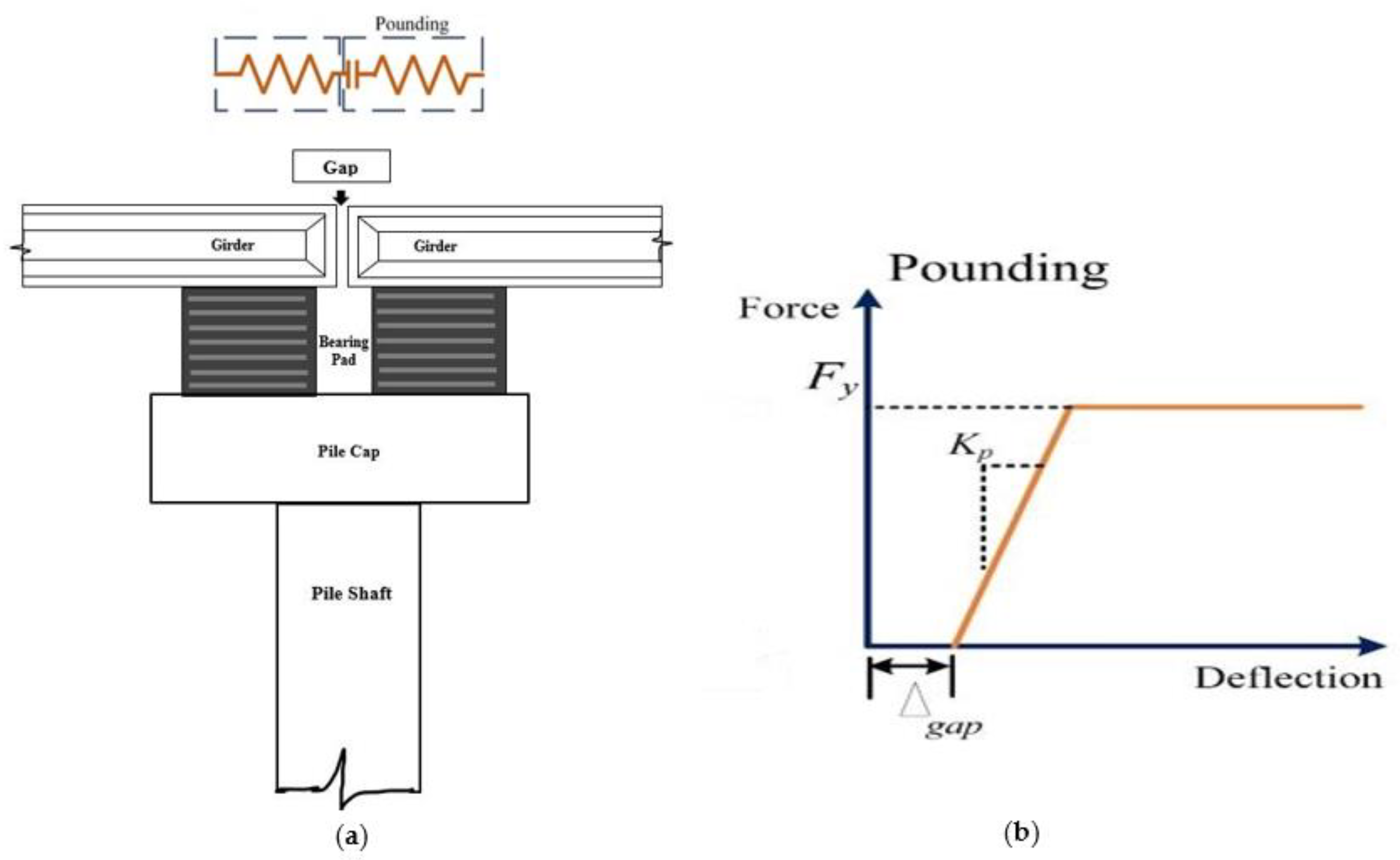
3.2.1. Bearing Pads
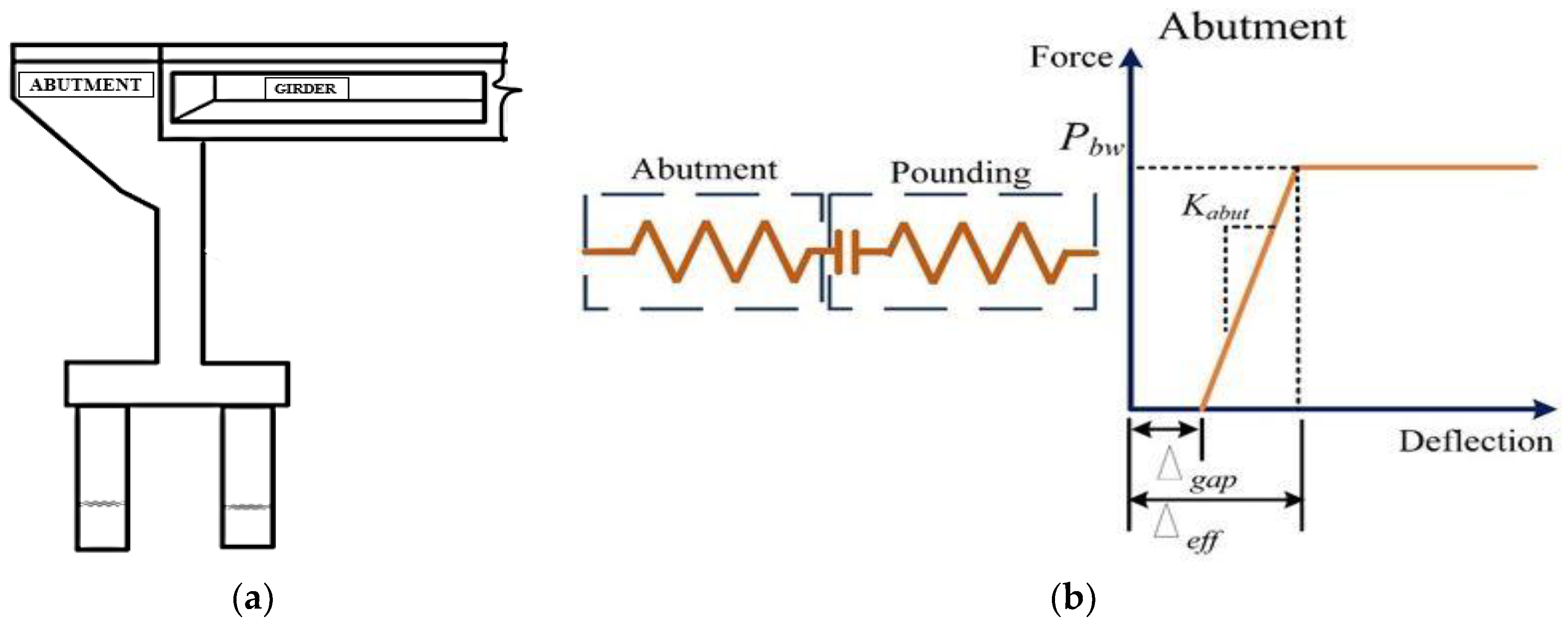
3.2.2. Abutments
3.3. Expansion Joint
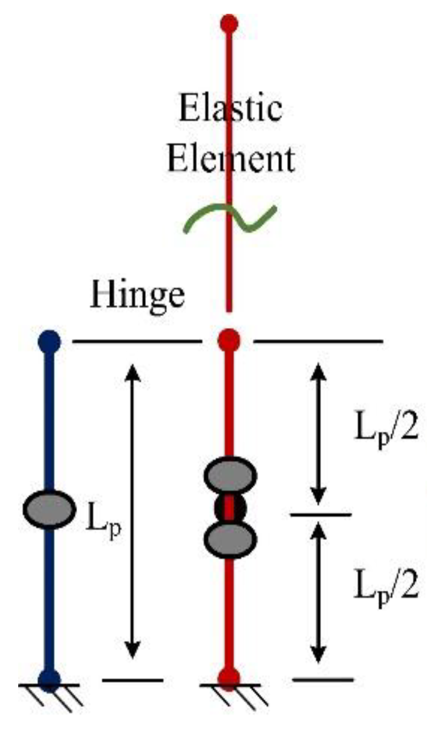
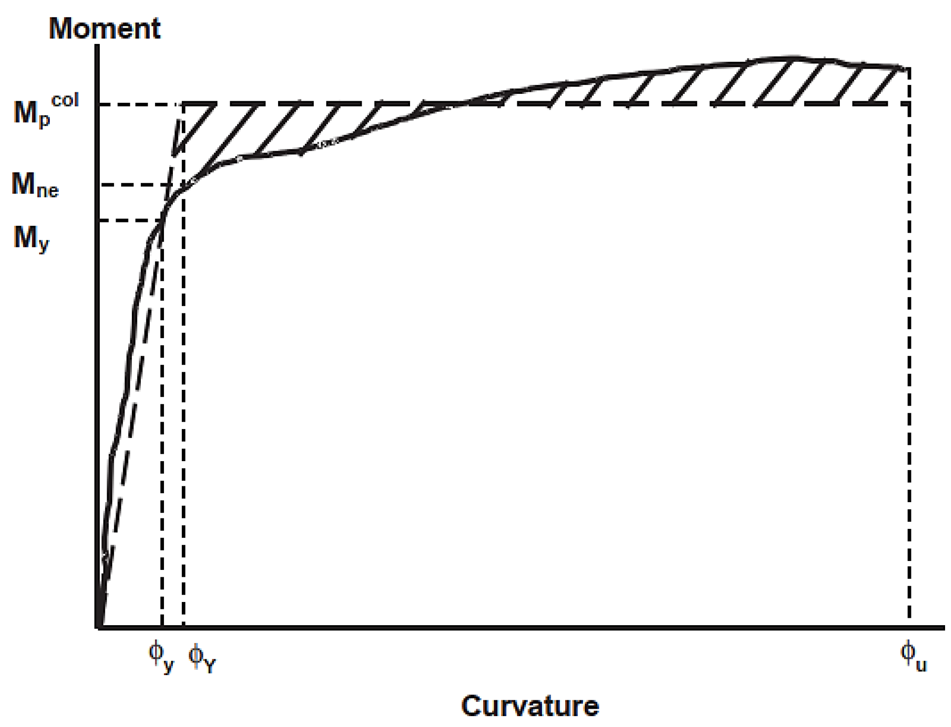
3.4. Plastic Hinges, Performance Limit and Bridge Piers
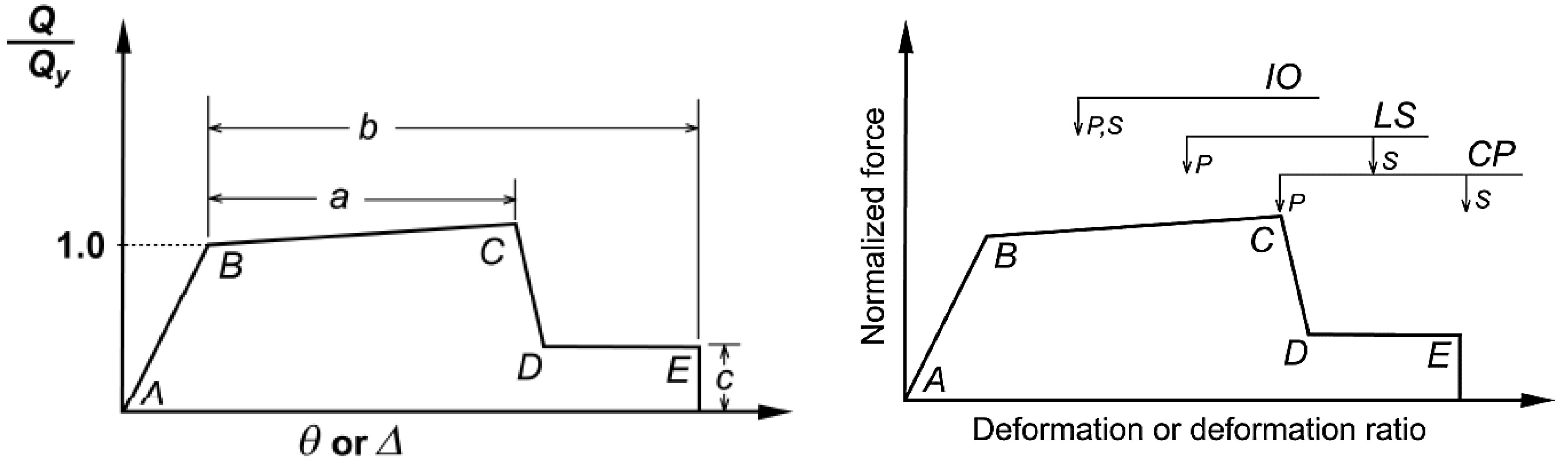
3.4.1. Performance Limits
3.4.2. Moment Curvature of Bridge Piers
ϕy = 0.00284 (1/m); ϕu = 0.1696 (1/m);
P = 1345 kN
ϕy = 0.00314 (1/m); ϕu = 0.171 (1/m);
P = 1468 kN
ϕy = 0.00288 (1/m); ϕu = 0.1706 (1/m);
P = 1453 kN
4. Response Modification Factor (R-Factor)
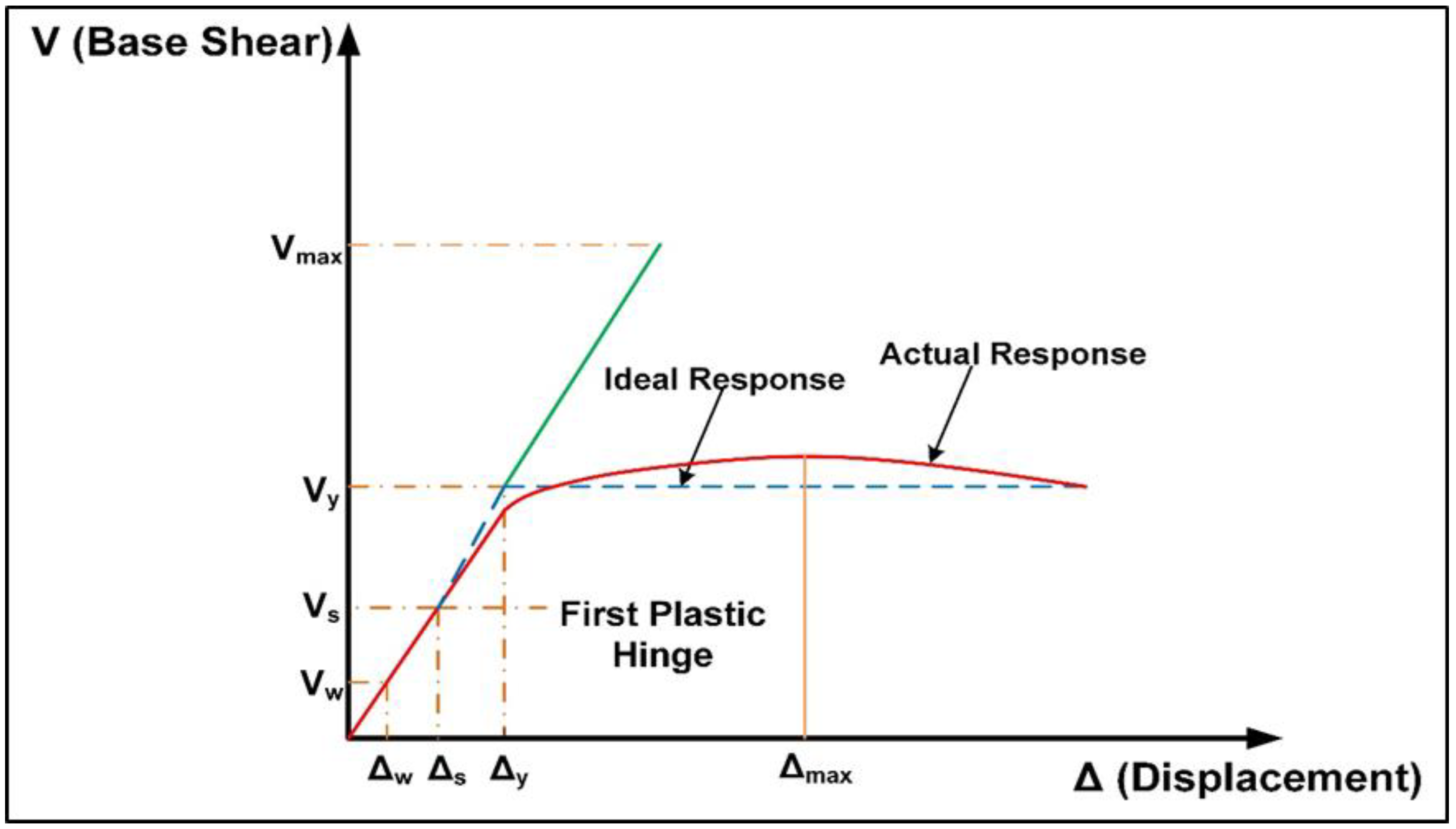
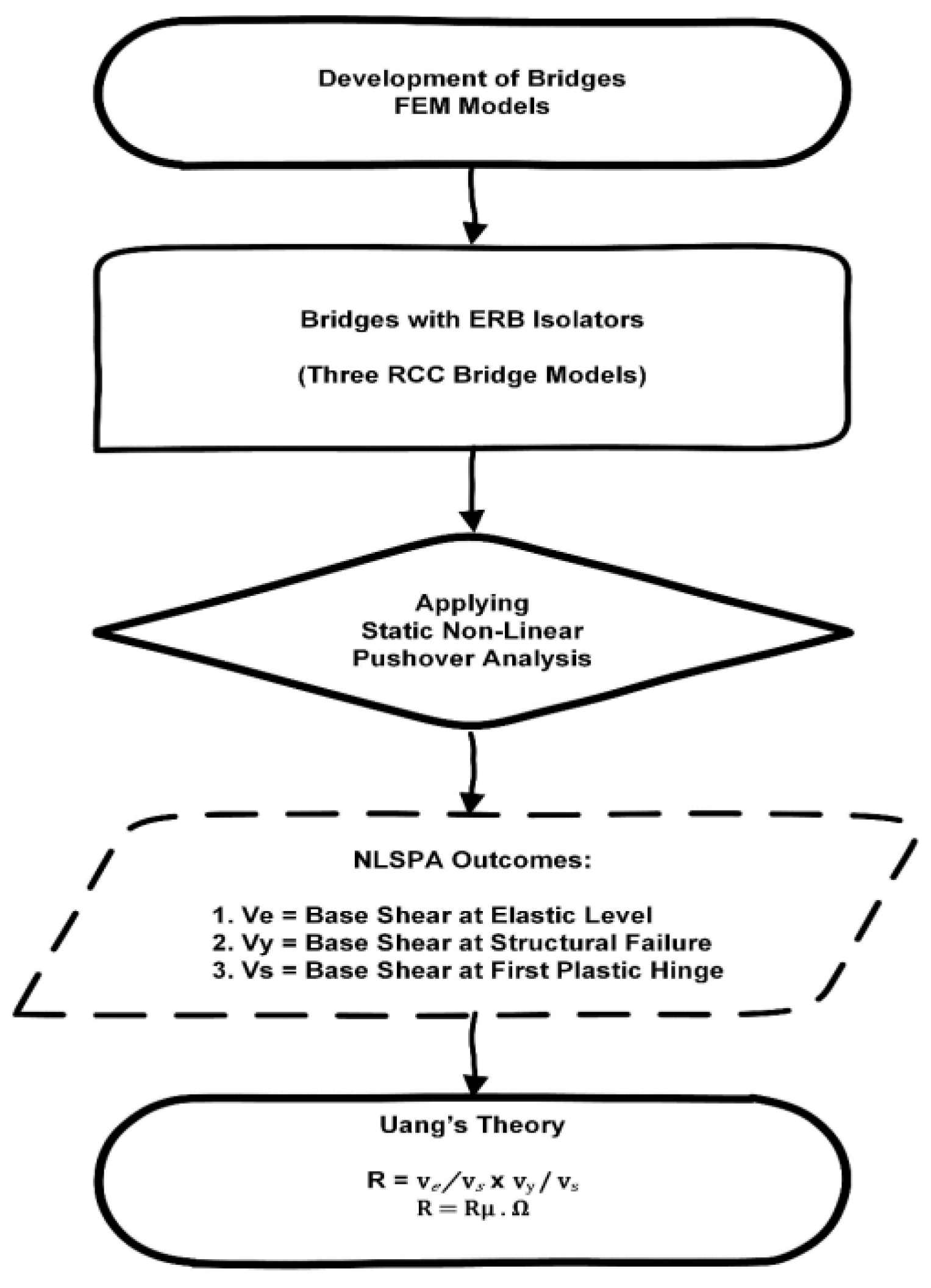
4.1. Uang’s Procedure R-Factor Coefficient Method
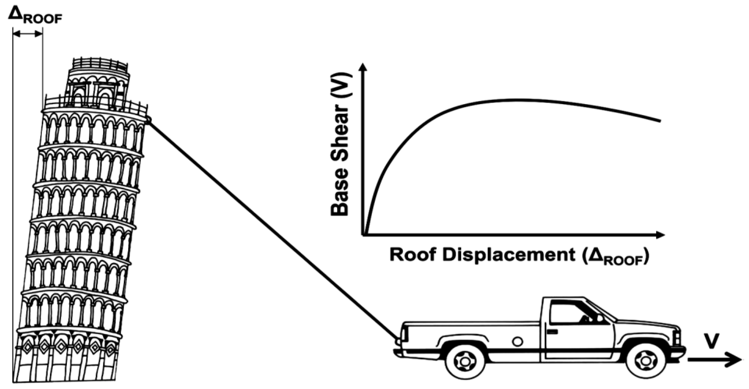
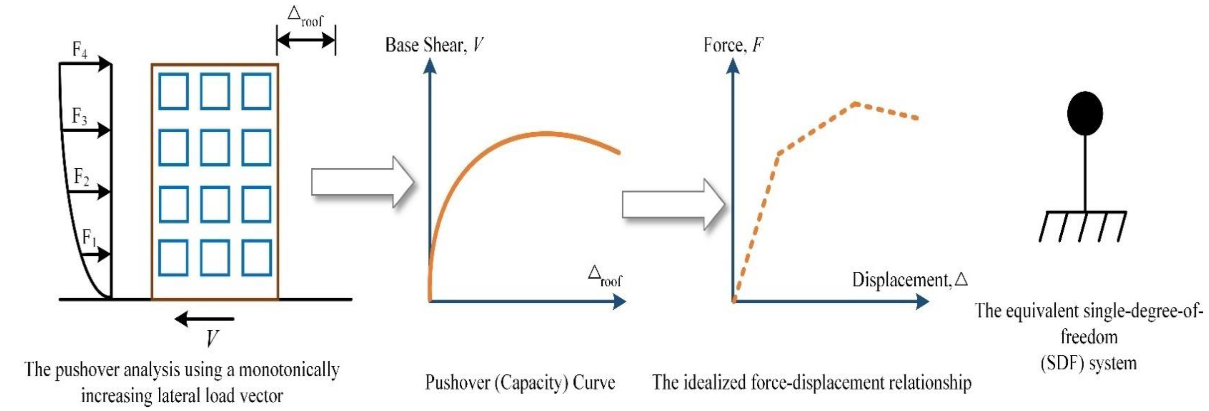
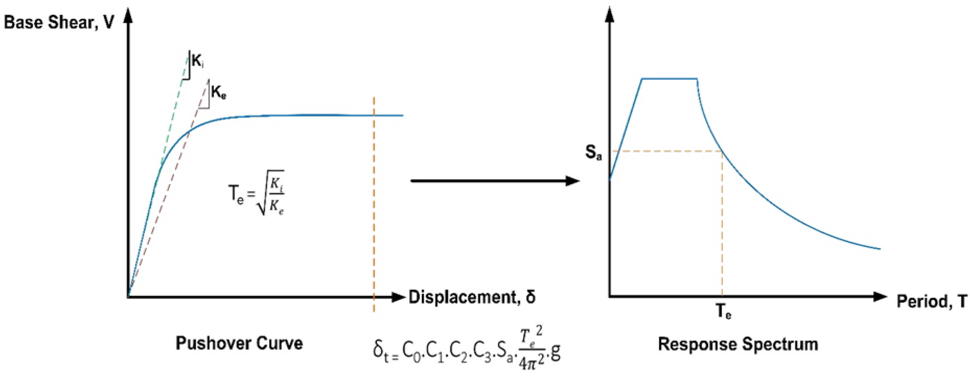
4.2. Nonlinear Static Pushover Analysis (NLSPA)
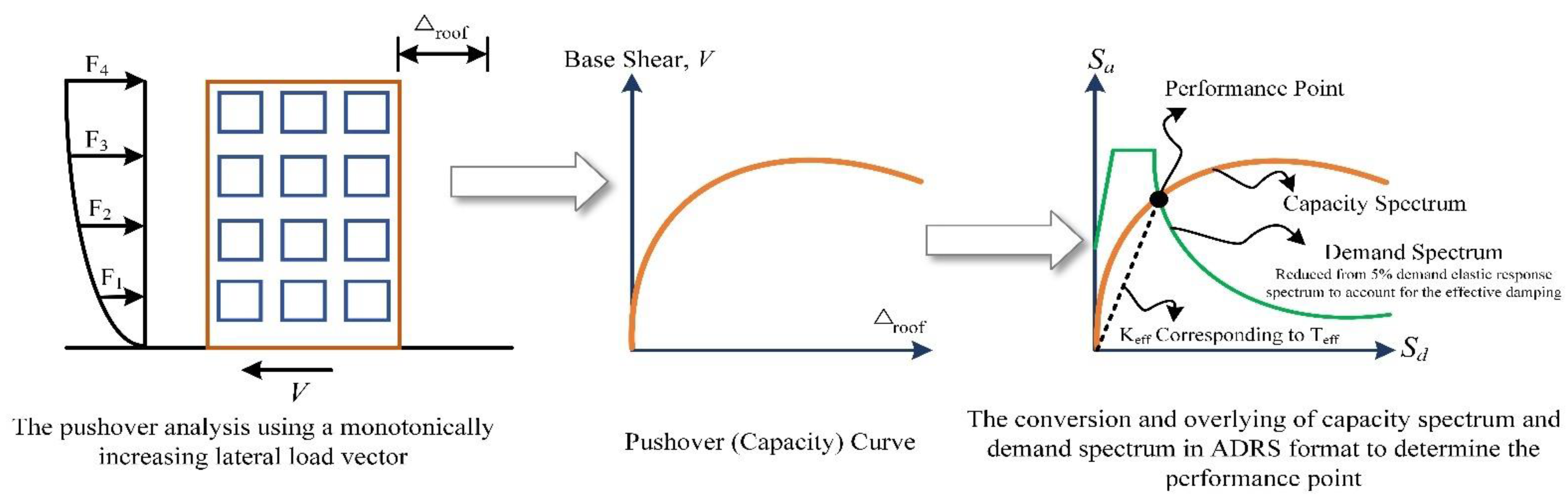
4.2.1. The Capacity Spectrum Method (CSM)
4.2.2. Displacement Coefficient Method (DCM)
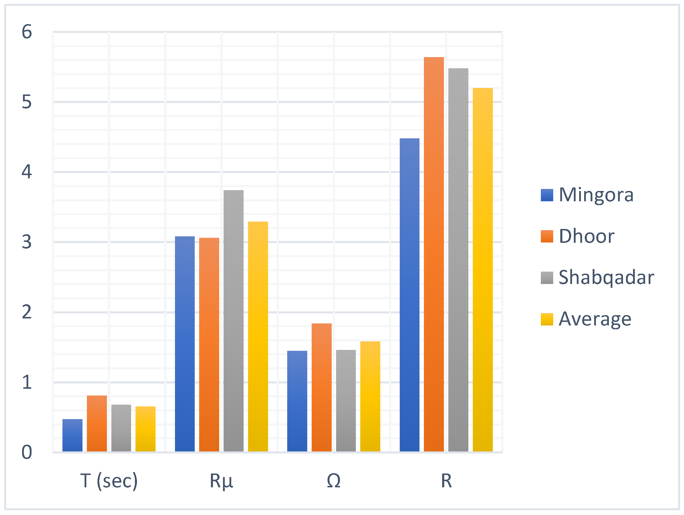
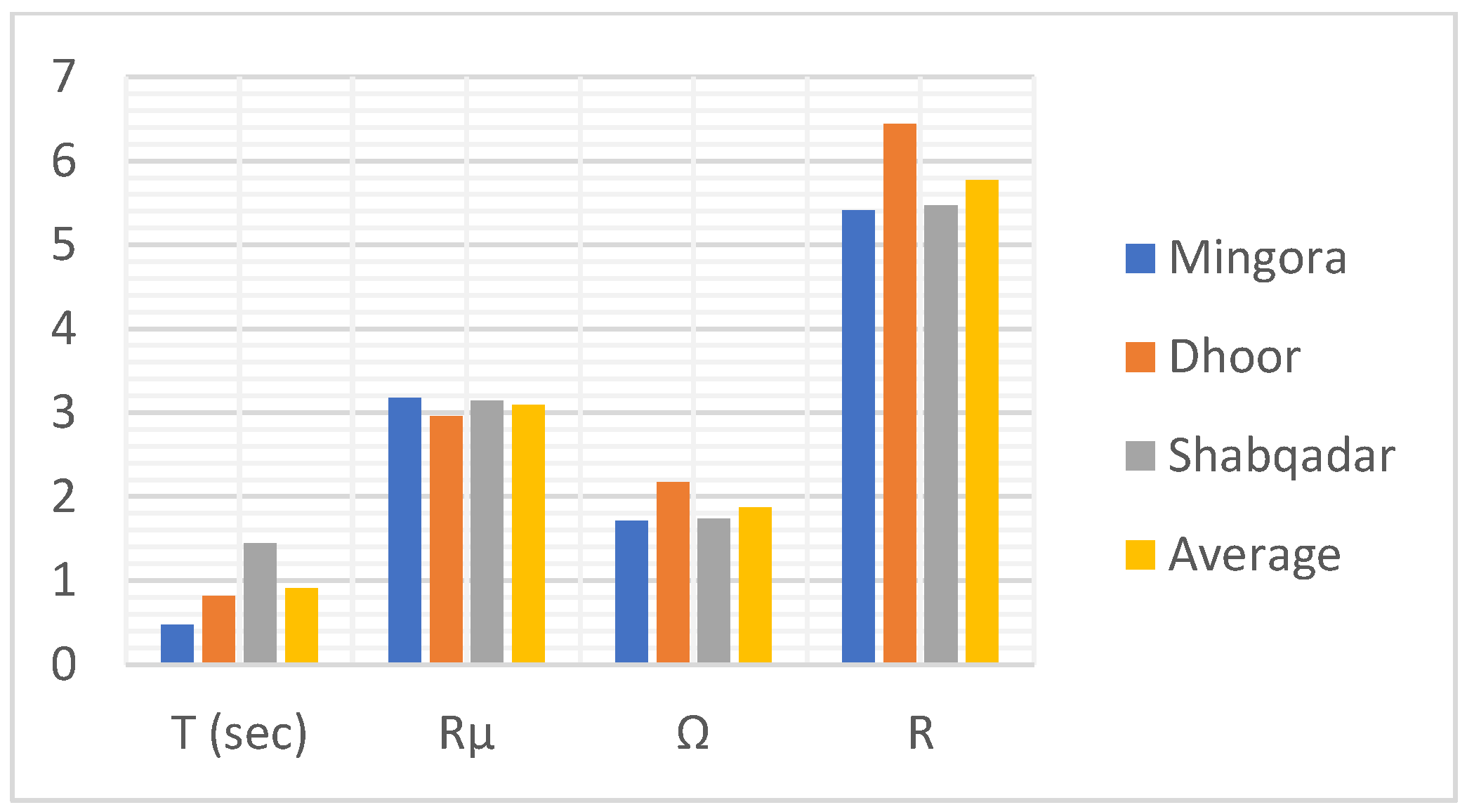
4.3. Response-Factor Computation
5. Conclusions
Author Contributions
Funding
Institutional Review Board Statement
Informed Consent Statement
Data Availability Statement
Conflicts of Interest
References
- Ali, S.M.; Khan, A.N.; Rahman, S.; Reinhorn, A.M. A survey of damages to bridges in Pakistan after the major earthquake of 8 October 2005. Earthq. Spectra 2011, 27, 947–970. [Google Scholar] [CrossRef]
- Kawashima, K. Seismic Isolation of Highway Bridges. J. JAEE 2004, 4, 283–297. [Google Scholar] [CrossRef]
- Sakellariadis, L.; Anastasopoulos, I.; Gazetas, G. Fukae bridge collapse (Kobe 1995) revisited: New insights. Soils Found. 2020, 60, 1450–1467. [Google Scholar] [CrossRef]
- Putra, R.; Riyono, W.A. Risk analysis of seismic bridge damage: Case study after Lombok and Palu earthquake. In E3S Web of Conferences 4th ICEEDM; EDP Sciences: Les Ulis, France, 2020; Volume 156, p. 03008. [Google Scholar]
- Memari, A.M.; Harris, H.G.; Hamid, A.A.; Scanlon, A. Ductility evaluation for typical existing R/C bridge columns in the eastern USA. Eng. Struct. 2005, 27, 203–212. [Google Scholar] [CrossRef]
- Kanamori, H. The energy release in great earthquakes. J. Geophys. Res. 1977, 82, 2981–2987. [Google Scholar] [CrossRef]
- Aye, M.N.; Kasai, A.; Shigeishi, M. An Investigation of Damage Mechanism Induced by Earthquake in a Plate Girder Bridge Based on Seismic Response Analysis: Case Study of Tawarayama Bridge under the 2016 Kumamoto Earthquake. Adv. Civ. Eng. 2018, 2018, 9293623. [Google Scholar] [CrossRef]
- Government of Pakistan Minstry of Housing and Works. Building Code of Pakistan; Government of Pakistan Minstry of Housing and Works: Islamabad, Pakistan, 2007.
- Ali, M. BCP SP-2007 BCP SP-2007 Preface; U.E.T Taxila: Rawalpindi, Pakistan, 2007. [Google Scholar]
- Khan, S.; Waseem, M. Earthquake seismic site response analysis by comparison between equivalent linear and nonlinear methods, a case study at Kohat and Muzaffarabad. J. Himal. Earth Sci. 2019, 52, 46–63. [Google Scholar]
- Khan, R.; Kumar, M.; Ahmed, M.; Rafi, M.; Lodi, S. Earthquake Damage Assessment of Bridges in Karachi. NED Univ. J. Res. 2015, 12, 45. [Google Scholar]
- Constantinou, M.; Quarshie, J. Response Modification Factors for Seismically Isolated Bridges; PAHO: New York, NY, USA, 1998; Available online: http://mceer.buffalo.edu/publications/catalog/reports/Response-Modification-Factors-for-Seismically-Isolated-Bridges-MCEER-98-0014.html (accessed on 3 November 1998).
- Federal Emergency Management Agency (FEMA). NEHRP Guidelines for the Seismic Rehabilitation of Buildings and NEHER Commentary on the Guidelines for the Seismic Rehabilitation of Buildings; Federal Emergency Management Agency (FEMA): Washington, DC, USA, 1997.
- International Conference of Building Officials. UBC-1997 Code. In Uniform Building. ‘Uniform Building Code’; International Conference of Building Officials: Whittier, CA, USA, 1997; ISBN 1884590896. [Google Scholar]
- Federal Emergency Management Agency (FEMA). ATC-1978 Applied Technology Council. Tentative Provisionsfor the Development ofSeismic Regulationsfor Buildings, National Science Foundation and National Bureau of Standards; Federal Emergency Management Agency (FEMA): Washington, DC, USA, 1984. [Google Scholar]
- Whittaker, A.; Hart, G.; Rojahn, C. Seismic response modification factors. J. Struct. Eng. 1999, 125, 438–444. [Google Scholar] [CrossRef]
- Ran, N. ATC 19 Structural Response Modifictaion Factors. 1995. Available online: https://www.atcouncil.org/pdfs/atc19toc.pdf (accessed on 24 May 1995).
- Gastineau, A.J.; Wojtkiewicz, S.F.; Schultz, A.E. Response Modification Approach for Safe Extension of Bridge Life. J. Bridg. Eng. 2012, 17, 728–732. [Google Scholar] [CrossRef]
- Gastineau, A.J.; Wojtkiewicz, S.F.; Schultz, A.E. Lifetime Extension of a Realistic Model of an In-Service Bridge through a Response Modification Approach. J. Eng. Mech. 2013, 139, 1681–1687. [Google Scholar] [CrossRef]
- Routledge, P.J.; Cowan, M.J.; Palermo, A. Low-damage detailing for bridges—A case study of Wigram-Magdala Bridge. In Proceedings of the 2016 NZSEE Conference, Christchurch, New Zealand, 14 November 2016; pp. 1–8. [Google Scholar]
- Warn, G.P.; Whittaker, A.S. Asce Property Modification Factors for Seismically Isolated Bridges. J. Bridg. Eng. 2006, 11, 371–377. [Google Scholar] [CrossRef]
- Çavdar, E.; Özdemir, G.; Karuk, V. Modification in Response of a Bridge Seismically Isolated with Lead Rubber Bearings Exposed to Low Temperature. Tek. Dergi 2022, 33, 1–24. [Google Scholar] [CrossRef]
- Zhang, F.; Li, S.; Wang, J.; Zhang, J. Effects of fault rupture on seismic responses of fault-crossing simply-supported highway bridges. Eng. Struct. 2020, 206, 110104. [Google Scholar] [CrossRef]
- Bergami, A.V.; Lavorato, D.; Fiorentino, G.; Nuti, C. Incremental Modal Pushover Analysis (IMPA) for bridges. Appl. Sci. 2021, 2911–2919. [Google Scholar] [CrossRef]
- Zhang, A.L.; Qiu, P.; Guo, K.; Jiang, Z.Q.; Wu, L.; Liu, S.C. Experimental study of earthquake-resilient end-plate type prefabricated steel frame beam-column joint. J. Constr. Steel Res. 2020, 166, 105927. [Google Scholar] [CrossRef]
- Kappos, A.J.; Paraskeva, T.S.; Moschonas, I.F. Response Modi fi cation Factors for Concrete Bridges in Europe. J. Bridg. Eng. 2013, 18, 1328–1335. [Google Scholar] [CrossRef]
- Zahrai, S.M.; Khorraminejad, A.; Sedaghati, P. Response modification factors of concrete bridges with different bearing conditions. Earthq. Struct. 2019, 16, 185–196. [Google Scholar] [CrossRef]
- Waseem, M.; Spacone, E. Fragility curves for the typical multi-span simply supported bridges in northern Pakistan. Struct. Eng. Mech. 2017, 64, 213–223. [Google Scholar] [CrossRef]
- Ali, S.M. Study of energy dissipation capacity of rc bridge columns under seismic demand. Ph.D. Thesis, University of Engineering and Technology, Peshawar, Pakistan, 2009. [Google Scholar]
- Uang, C.-M. Establishing R (or Rw) and Cd factors for building seismic provisions. J. Struct. Eng. 1991, 117, 19–28. [Google Scholar] [CrossRef]
- Aviram, A.; Mackie, K.; Stojadinovic, B. Guidelines for Nonlinear Analysis of Bridge Structures in California; Pacific Earthquake Engineering Research Center: Berkeley, CA, USA, 2008. [Google Scholar]
- Akogul, C.; Celik, O. Effect of Elastomeric Bearing Modeling Parameters on the Seismis Design of RC Highway Bridges with Precast Concrete Girders. In Proceedings of the 14th World Conference on Earthquake Engineering, Beijing, China, 12–17 October 2008; Available online: https://www.researchgate.net/publication/265930567_Effect_of_elastomeric_bearing_modeling_parameters_on_the_Seismis_design_of_RC_highway_bridges_with_precast_concrete_girders (accessed on 17 October 2008).
- Caltrans Seismic Design Criteria, Version 1.3; Caltrans: Sacramento, CA, USA, 2004.
- Mander, J.B.; Priestley, M.J.N.; Park, R. Theoretical stress-strain model for confined concrete. J. Struct. Eng. 1989, 114, 1804–1826. [Google Scholar] [CrossRef]
- Tortolini, P.; Petrangeli, M.; Lupoi, A. Criteri per la verifica e la sostituzione degli appoggi in neoprene di viadotti esistenti in zona sismica. In Proceedings of the 14th Italian Conference on Earthquake Engineering, Bari, Italy, 30 August–3 September 2011; Available online: https://www.researchgate.net/publication/266941512 (accessed on 17 October 2008).
- Malhotra, V.M.; Mehta, P.K. Standard specifications. In Pozzolanic and Cementitious Materials; CRC Press: Boca Raton, FL, USA, 2006; p. 871. [Google Scholar] [CrossRef]
- Yazdani, N.; Eddy, S.; Cai, C.S. Effect of bearing pads on precast prestressed concrete bridges. J. Bridg. Eng. 1999, 5, 224–232. [Google Scholar] [CrossRef]
- Shafiei-tehrany, R. Nonlinear Dynamic and Static Analysis of I-5 Ravenna Bridge. Ph.D. Thesis, Washington State University, Washington, WA, USA, 2008. [Google Scholar]
- Muthukumar, S. A Contact Element Approach with Hysteresis Damping for the Analysis and Design of Pounding in Bridges; Georgia Institute of Technology: Atlanta, GA, USA, 2003. [Google Scholar]
- Caltrans Seismic Design Criteria, Version 1.7; Caltrans: Sacramento, CA, USA, 2013.
- Hakim, R.A.; Alama, M.S.; Ashour, S.A. Seismic Assessment of RC Building According to ATC 40, FEMA 356 and FEMA 440. Arab. J. Sci. Eng. 2014, 39, 7691–7699. [Google Scholar] [CrossRef]
- Favvata, M.J.; Naoum, M.C.; Karayannis, C.G. Seismic Evaluation of Infilled RC Structures with Nonlinear Static Analysis Procedures. In Proceedings of the 15th World Conference on Earthquake Engineering, Lisbon, Portugal, 24–28 September 2012. [Google Scholar]
- Abdi, H.; Hejazi, F.; Jaafar, M.S. Response modification factor—Review paper. IOP Conf. Ser. Earth Environ. Sci. 2019, 357, 1–16. [Google Scholar] [CrossRef]
- Building Seismic Safety Council; Washington, D. NEHRP Recommended Provisions for Seismic Regulations for New Buildings; U.S. Department of Homeland Security: Washington, CA, USA, 1988.
- Zafar, A. Response Modification Factor of Reinforced Concrete Moment Resisting Frames in Developing Countries. Master’s Thesis, University of Illinois at Urbana-Champaign, Champaign, IL, USA, 2009. [Google Scholar]
- Nassar, A.A.; Krawinkler, H. Seismic demands for SDOF and MDOF systems, Report No. 95. Stanford Univ. 1991, 204, 12–45. [Google Scholar]
- Krawinkler, H.; Seneviratna, G.D.P.K. Pros and cons of a pushover analysis of seismic performance evaluation. Eng. Struct. 1998, 20, 452–464. [Google Scholar] [CrossRef]
- Fajardo, K.N.; Blázquez, A. FEMA 356 Preestándar y Comentario Para la Rehabilitación Sísmica de Edificios; Interreg Poctefa: Spain, France, 2000; p. 519. [Google Scholar]
- Najam, F.A. Nonlinear Static Analysis Procedures for Seismic Performance Evaluation of Existing Buildings—Evolution and Issues. In International Congress and Exhibition Sustainable Civil Infrastructures: Innovative Infrastructure Geotechnology; Springer: Cham, Swizerland, 2018. [Google Scholar] [CrossRef]
- ATC 40—Seismic evaluation and retrofit of concrete buildings. Available online: https://www.atcouncil.org/pdfs/atc40toc.pdf (accessed on 30 November 1996).
- FEMA-440, Improvement of Nonlinear Static Seismic Analysis Procedures. Available online: https://store.atcouncil.org/index.php?dispatch=attachments.getfile&attachment_id=123 (accessed on 29 June 2005).


| Bridge ID | Bridge 1 | Bridge 2 | Bridge 3 |
|---|---|---|---|
| Bridge name | Shabqadar | Dhoor | Mingora |
| No. of spans | 10 | 10 | 3 |
| Span length (mm) | 10 × 25,000 | 10 × 30,100 | 3 × 16,100 |
| Bridge width (mm) | 11,000 | 9900 | 11,200 |
| No. of girders | 4 | 4 | 4 |
| Girder material | Concrete | Concrete | Concrete |
| No. of piers | 4 | 3 | 3 |
| Pier diameter (mm) | D = 1200 | D = 1200 | D = 1200 |
| Sr. # | Bridge Name | Spans | Bearing Pad Area (Ab, mm) | Neoprene Thickness (H, mm) | Horizontal Stiffness (Kh, kN/mm) |
|---|---|---|---|---|---|
| 1. | Charsadda Bridge | 10 | 400 × 600 | 69 | 4706 |
| 2. | Dhoor Bridge | 10 | 500 × 500 | 82 | 3906.3 |
| 3. | Mingora Bridge | 03 | 400 ×550 | 38 | 5789 |
| Immediate Occupancy | Damage Control | Life Safety | Structural Stability |
|---|---|---|---|
| 0.01 | 0.01–0.02 | 0.02 | 0.33 Vi/Pi |
| Trans. Reinf. | Modeling Parameter | Plastic Rotation Limit | ||||||
|---|---|---|---|---|---|---|---|---|
| a | b | c | Immediate Occupancy | Life Safety | Structural Stability | |||
| ≤0.1 | C | ≤3 | 0.02 | 0.03 | 0.2 | 0.005 | 0.001 | 0.020 |
| ≤0.1 | C | ≥6 | 0.016 | 0.024 | 0.2 | 0.005 | 0.001 | 0.015 |
| ≥0.4 | C | ≤3 | 0.015 | 0.025 | 0.2 | 0.003 | 0.005 | 0.015 |
| ≥0.4 | C | ≥6 | 0.012 | 0.02 | 0.2 | 0.003 | 0.005 | 0.010 |
| α (%) | a | b |
|---|---|---|
| 0 | 1 | 0.42 |
| 2 | 1 | 0.37 |
| 10 | 0.8 | 0.29 |
| T | a | b | C (T,α) | µ | Rµ | Δm | Δy | Ω | R-Factor |
|---|---|---|---|---|---|---|---|---|---|
| 0.47 | 1 | 0.42 | 1.20 | 3.52 | 3.18 | 120.56 | 34.59 | 1.71 | 5.41 |
| T | a | b | C (T,α) | µ | Rµ | Δm | Δy | Ω | R-Factor |
|---|---|---|---|---|---|---|---|---|---|
| 0.47 | 1 | 0.42 | 1.20 | 3.39 | 3.08 | 118.65 | 34.501 | 1.45 | 4.48 |
| T | a | b | C (T,α) | µ | Rµ | Δm | Δy | Ω | R-Factor |
|---|---|---|---|---|---|---|---|---|---|
| 1.44 | 1 | 0.42 | 0.88 | 2.97 | 3.14 | 97.14 | 32.68 | 1.74 | 5.47 |
| T | a | b | C (T,α) | µ | Rµ | Δm | Δy | Ω | R-Factor |
|---|---|---|---|---|---|---|---|---|---|
| 0.677 | 1 | 0.42 | 1.02 | 3.79 | 3.74 | 130.58 | 34.43 | 1.46 | 5.48 |
| T | a | b | C (T,α) | µ | Rµ | Δm | Δy | Ω | R-Factor |
|---|---|---|---|---|---|---|---|---|---|
| 0.813 | 1 | 0.42 | 0.966 | 2.92 | 2.96 | 179.606 | 61.78 | 2.17 | 6.44 |
| T | a | b | C (T,α) | µ | Rµ | Δm | Δy | Ω | R-Factor |
|---|---|---|---|---|---|---|---|---|---|
| 0.808 | 1 | 0.42 | 0.966 | 1.83 | 1.84 | 120.18 | 65.50 | 3.06 | 5.64 |
| X-Dir | Bridge.1 | Bridge.2 | Bridge.3 | Average |
|---|---|---|---|---|
| Name | Mingora | Dhoor | Shabqadar | |
| T (s) | 0.472362 | 0.808817 | 0.67773 | |
| Rμ | 3.08 | 3.06 | 3.74 | 3.29 |
| Ω | 1.45 | 1.84 | 1.46 | 1.58 |
| R | 4.48 | 5.64 | 5.48 | 5.20 |
| Y-Dir | Bridge.1 | Bridge.2 | Bridge.3 | Average |
|---|---|---|---|---|
| Name | Mingora | Dhoor | Shabqadar | |
| T (s) | 0.473977 | 0.81375 | 1.4434 | |
| Rμ | 3.18 | 2.96 | 3.14 | 3.09 |
| Ω | 1.71 | 2.17 | 1.74 | 1.87 |
| R | 5.41 | 6.44 | 5.47 | 5.77 |
Publisher’s Note: MDPI stays neutral with regard to jurisdictional claims in published maps and institutional affiliations. |
© 2022 by the authors. Licensee MDPI, Basel, Switzerland. This article is an open access article distributed under the terms and conditions of the Creative Commons Attribution (CC BY) license (https://creativecommons.org/licenses/by/4.0/).
Share and Cite
Butt, M.J.; Waseem, M.; Sikandar, M.A.; Zamin, B.; Ahmad, M.; Muayad Sabri Sabri, M. Response Modification Factors for Multi-Span Reinforced Concrete Bridges in Pakistan. Buildings 2022, 12, 921. https://doi.org/10.3390/buildings12070921
Butt MJ, Waseem M, Sikandar MA, Zamin B, Ahmad M, Muayad Sabri Sabri M. Response Modification Factors for Multi-Span Reinforced Concrete Bridges in Pakistan. Buildings. 2022; 12(7):921. https://doi.org/10.3390/buildings12070921
Chicago/Turabian StyleButt, Muhammad Jamal, Muhammad Waseem, Muhammad Ali Sikandar, Bakht Zamin, Mahmood Ahmad, and Mohanad Muayad Sabri Sabri. 2022. "Response Modification Factors for Multi-Span Reinforced Concrete Bridges in Pakistan" Buildings 12, no. 7: 921. https://doi.org/10.3390/buildings12070921
APA StyleButt, M. J., Waseem, M., Sikandar, M. A., Zamin, B., Ahmad, M., & Muayad Sabri Sabri, M. (2022). Response Modification Factors for Multi-Span Reinforced Concrete Bridges in Pakistan. Buildings, 12(7), 921. https://doi.org/10.3390/buildings12070921