1. Introduction
The school building studied in this paper was equipped by a seismic recording system within the network for monitoring public buildings, bridges and dams, the Seismic Observatory of Structure (OSS) of the Italian Department of Civil Protection (DPC). As reported with more details in [
1], the seismic responses of structures are recorded for both scientific and civil protection purposes: acceleration measures are acquired at each floor in real time and processed in the OSS central server in Rome, assessing possible damage (which can be extended to buildings having similar construction typology) based on experimental inter-storey drifts. All recorded data are shared automatically via website with the technical/scientific community for both improving the knowledge of the real structural behaviour under earthquakes and providing background for technical regulations. OSS measured quantities are also a quick alert for DPC, which can accordingly mobilize the Italian Civil Protection System, including regional and municipal local authorities and operational structures as the fire brigade, Red Cross, police, volunteers, etc. Prior to the installation of the monitoring system, a survey of the monitored structures is performed, including structure design, soil properties, photographic reports, assessment of geometric and mechanic properties, development and analysis of finite element models (optimized by comparison with experimental data), and vulnerability analysis.
Between August and November 2016, three major earthquake events occurred in Central Italy. The first event (magnitude (M) = 6.1) occurred on 24 August 2016, the second (M = 5.9) occurred on 26 October 2016, and the third (M = 6.5) occurred on 30 October 2016. Each event was followed by numerous after-shocks, some exceeding M = 5. A comprehensive description of the sequence is out of the scope of this paper. A large body of literature is available about this topic; to cite only one paper, in [
2], a synthesis of the observations of two post-event reconnaissance teams is reported. Analyses of the damage patterns in several towns, like Amatrice, can be found in [
3]: in particular, the evolution of damage due to the seismic sequence within each vulnerability class of buildings is reported.
Several papers have been devoted to the analysis of the structural response and damage observed during the 2016 seismic sequence [
4,
5,
6,
7,
8,
9,
10,
11,
12,
13,
14,
15,
16,
17,
18,
19,
20,
21]. They used different computational models and tools (commercial or research codes) based on a wide variety of approaches, including nonlinear, linear with kinematic constraints, non-smooth contact dynamics, macroelements, and seismic regulations codified procedures. One group [
4,
5,
6,
7,
8,
9,
10,
11] is devoted to non-monitored structures; they are limited to a prediction of structure response and have highlighted the capacity of the computational techniques adopted in satisfactorily representing the real damage scenario, even if from a qualitative point of view. More interesting is the second group [
12,
13,
14,
15,
16,
17,
18,
19,
20,
21], which is devoted to the analysis of monitored structures, some of which are included in the OSS set. For these structures, as the one studied in this paper, records of dynamic quantities due to environmental and seismic excitations are available.
The papers [
12,
16,
20,
21] addressed a masonry school building in Visso town and showed that the measured acceleration signals are well reproduced by a nonlinear commercial code. The papers [
13,
15] examined data recorded by the monitoring systems of three buildings, which were used to study the phenomenon of frequency and damping wandering during strong motion. In [
14], the experimental results were used to calibrate the numerical model in order to assess strengthening interventions. The papers [
17,
19] focused on school buildings outside the epicentral area, slightly impacted by the 2016 seismic sequence. The paper [
18] addressed a base isolated building; the authors observed that the comparison between the recorded seismic accelerations and the corresponding accelerations obtained from a numerical model showed a good correspondence in one direction; in the other direction, characterized by a high-frequency response attributed to the presence of an elevator shaft, the acceleration peaks are underestimated by the numerical model.
As is well known, structural health monitoring (SHM) techniques can be applied on data gathered from a seismic monitoring system. Even if a comprehensive review of SHMs is outside the aim of this paper, the classification reported in [
22] is of interest, where the approaches proposed in the literature are distinguished as being either model-based or signal-based. In the former approaches, damage is recognized through tracking variations in the simulated measurements from a structural model, and specific parameters of this model are updated under the system’s responses, as discussed, for example, in [
23]. The latter approaches rely on statistical analysis and assess the system’s response independently; therefore, they do not require additional information concerning the structure’s physical properties and parameters. One of the main issues of signal-based techniques is the limitation of the number of response quantities. As discussed in the following, combining experimental and numerical results, available response quantities can be expanded in order to obtain much information at the local level, thus allowing the estimation of damage on all relevant structural elements.
This paper is focused on the interpretation of data gathered by the OSS monitoring system installed on a school building in Amatrice while also taking advantage of interpretative numerical models. First, a linear finite element model is used for the simulation of small amplitude vibrations in order to obtain a reliable dynamic characterization of the structure’s initial conditions. Some relevant quantities of the recorded motion are selected to describe the experimental dynamic behaviour under the seismic excitation. As far as the estimation of damage degree, at present, this is performed with a simplified approach, where the maximum recorded inter-storey drifts are compared with literature reference values established for different construction typologies (masonry, reinforced concrete RC). This approach has been improved on the basis of measured quantities and the specific characteristics of the structure under study: the recorded displacements are applied to a nonlinear finite element model of the structure, and the numerical results, which satisfactorily describe the experimental evidence, furnish reliable quantification of local damage. This approach is also useful in a SHM perspective, because it allows us to expand the experimental data set and to gather information at the local level on a great number of structural elements.
2. Description of the Building Aggregate
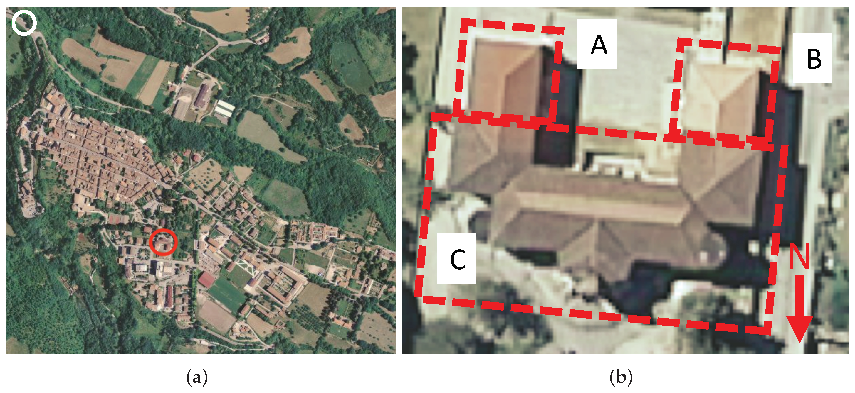
The school building aggregate studied in this paper, belonging to a typology widely studied in a seismic perspective in the last years [
24,
25], is located near the centre of Amatrice. The aerial view of the aggregate is reported in
Figure 1a, while in
Figure 1b, the three buildings belonging to the aggregate are evidenced. The main school building C was constructed from 1933 to 1936; the structural typology was masonry made by irregular stones interrupted at regular distance by horizontal layers of clay bricks. The original wooden roof was substituted in the 1970s by ribbed slabs, similar to those of the floors. Building C has two levels above ground and one level partly under ground. RC buildings A and B were added in 1990 and 2000, respectively. Both buildings A and B have two levels above ground, while building B also has one level under ground. The floor slabs of buildings A and B were made by hollow clay bricks and RC joists; the roof slab of building A consists of corrugated steel sheets supported by steel trusses, while for building B’s roof, the same typology of floors was used. Despite the fact that masonry and RC buildings were separated by structural joints, the roof did not have evident discontinuity of the tiles.
In Italy, three seismic zones exist according to both historical and modern regulations (Zone 1 corresponds to locations with the highest seismicity), not considering Zone 4, where the seismic hazard is negligible. Amatrice was classified as seismic Zone 2 starting in 1915. In 1983, Zone 2 was confirmed, while in 2003, Zone 1 was enforced. Until 2003, seismic action was described using conventional parameters without physical meaning; starting in 2003, the seismic action began to be described using uniform hazard spectra. Thus, it is reasonable to assume that all buildings A, B and C have been designed according to the actions corresponding to seismic Zone 2; at that time, the structural design under seismic actions was performed by applying to the building a system of equivalent horizontal loads and performing allowable stress checks. Starting from 1984, and this is significant only for buildings A and B, seismic codes required a 20% increment of the horizontal loads for buildings characterized by a higher level of risk, such as school buildings, if compared to ordinary ones.
At the end of 2009, a seismic vulnerability assessment of building C was performed, leading to a seismic reliability factor (i.e., the displacement capacity/demand ratio) in the range between 0.4 and 0.6; the variability was due to different assumptions for the masonry characteristics. For buildings A and B, the estimate of the seismic reliability factor was about 0.4. The vulnerability assessment was conducted according to the Italian seismic regulation [
26] with reference to a 712-year return period seismic action, greater than the 475-year return period applicable for ordinary buildings; the reference limit state was similar to the so-called life safety according to modern international seismic codes.
In 2012, structural interventions were made to buildings A and B: the columns were reinforced with fiber-reinforced polymer (FRP) material, and plastic fiber-reinforced plaster was applied to external infills and internal partitions in order to prevent the falling of debris in case of an earthquake.
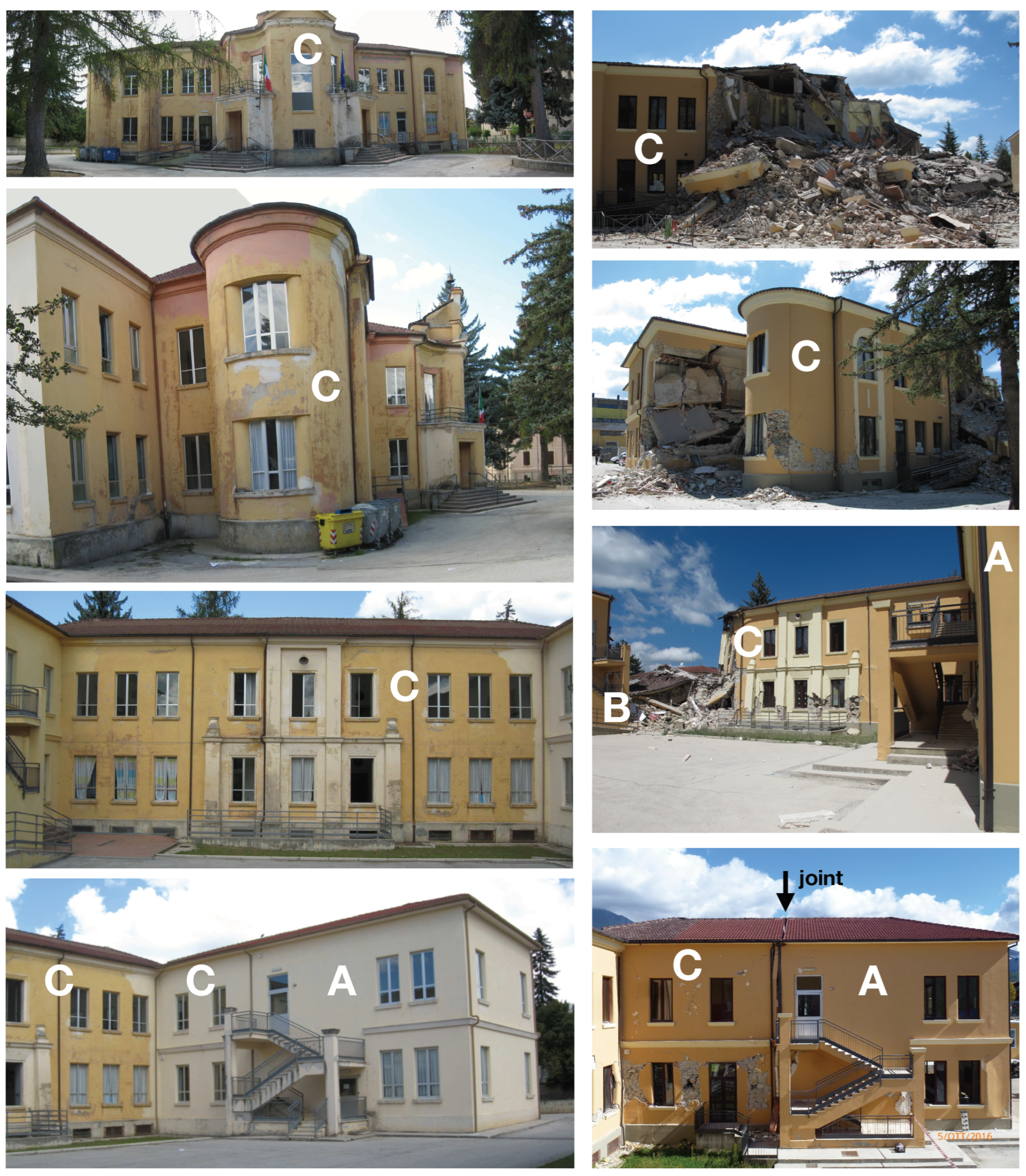
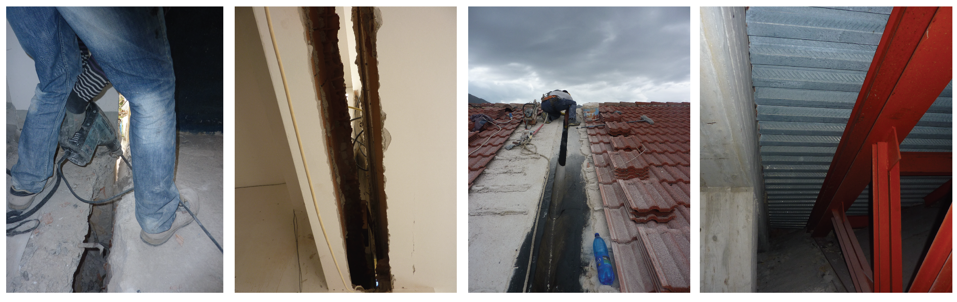
After the main shock of the 24 August 2016 earthquake, in the following simply denoted as the 2016 earthquake, the conditions of the buildings were as depicted in
Figure 2. Building C underwent a partial collapse, involving the portion of the building having an underground level (
Figure 2 and Figure 4). The remaining portion of the building showed very heavy damage, with several diagonal cracks in the walls and an overturning of a facade owing to out-of-plane actions. Buildings A and B showed relevant damage to infills and partitions without collapse and moderate damage to structural elements. Damage was also evident to the joints between buildings C and A, where the tiles collapsed and a 15 cm opening appeared (see bottom picture of
Figure 2).
Special attention must be paid to the dimensions of the structural joints between buildings A, B and C. At the time of the construction of both buildings A and B, a minimum joint dimension of 1% of the height with respect to the foundations was enforced. This corresponds to nearly 10 cm for building A and 12 cm for building B. According to the code [
26] applicable for the 2012 interventions, the 1% minimum joint dimension must be multiplied by a factor depending on the site seismicity, corresponding to a 30% increment of the previously reported values. In 2011, some tests on all buildings concerning material properties, structural details, and, in particular, the joints between buildings C, A and B were performed by DPC. As documented in
Figure 3 during the 2012 seismic upgrading of buildings A and B, the structural configurations of the joints were checked at all levels. At the roof level, in order to avoid damage to the tile layer in ordinary conditions, a weak connection was built to sustain the nonstructural elements. The performance of the structural joints will be discussed in the following on the basis of the recorded quantities.
3. Description of the Monitoring System
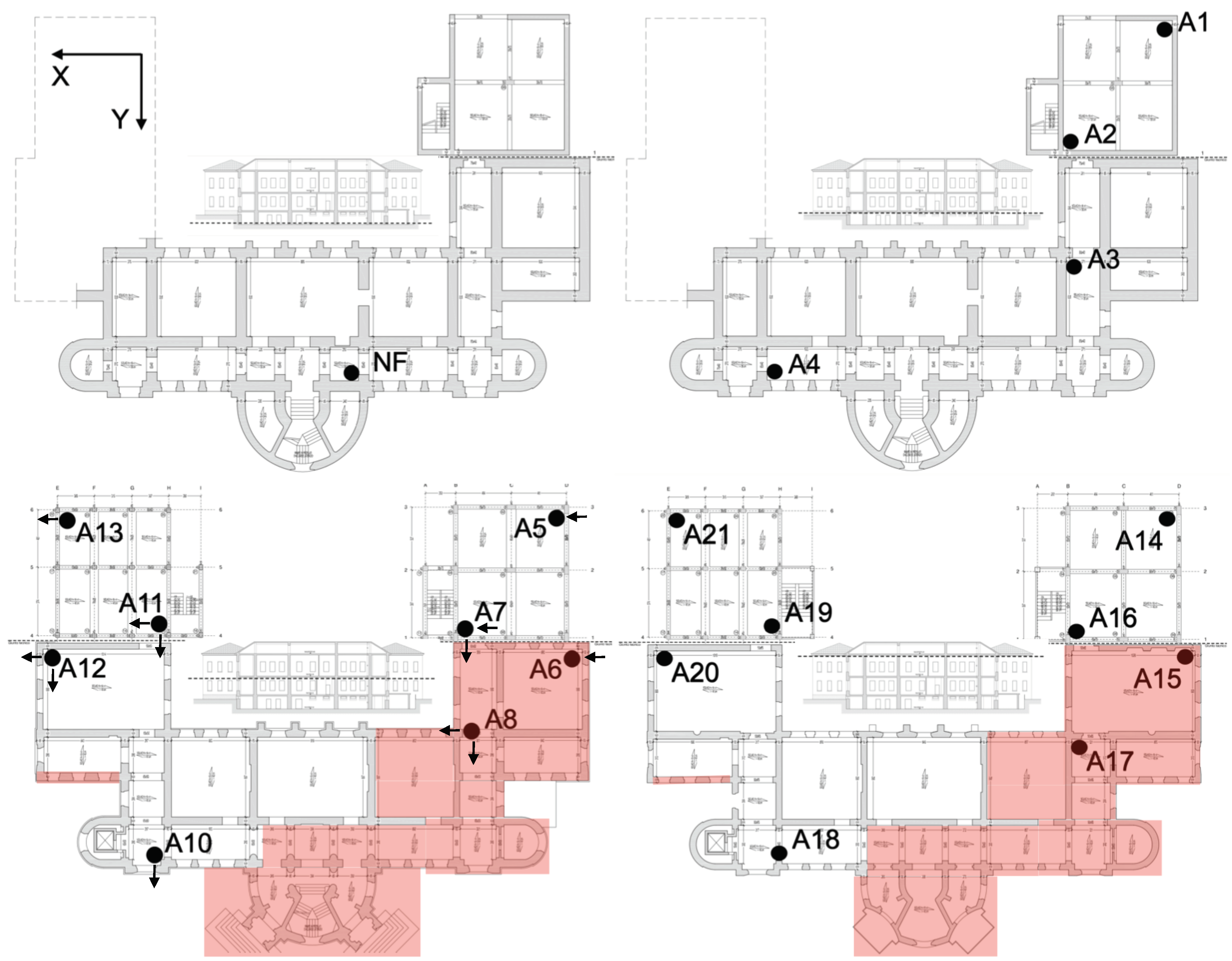
The monitoring system installed in 2010 on the aggregate studied in this paper is composed of 1 digital recording unit, 21 accelerometers (1 triaxial, 10 bi-directional, 10 mono-directional), 1 GPS receiving unit for UTC synchronisation, and 1 ADSL modem for communications with DPC server; all sensors are connected to the local recording unit by cables. The locations of the sensors are reported in
Figure 4. The number and locations of the components were selected in order to describe the floor plane motion in a realistic manner. The floors of buildings A and B can be reasonably considered as rigid, while for building C, a deformation of the floors can be expected. Thus, for this building more components were deployed, as depicted in
Figure 4. In particular, the sensor locations were selected in order to allow the definition of three different rigid body constraints, as discussed in the following.
The nominal full-scale of the NF sensor is ±0.5 g. For the other sensors, the nominal full-scale is ±1 g. Accelerations 33% greater than the above-reported nominal full-scale values can be recorded by the system. Indeed, a 7.5 V electric current corresponds to the nominal full-scale, while the digitizer is capable of recording up to 10 V, i.e., 33% more than 7.5 V. Thus, when the acceleration exceeds the nominal full-scale, the digitizer is still capable of recording it up to ±0.66 g for NF and ±1.33 g for the remaining ones.
4. Experimental Modal Analysis and Linear Model Updating
Prior to discussing the behaviour of the buildings under the 2016 destructive earthquake, it is useful to highlight their dynamical properties gathered from experimental modal analyses. As previously discussed, in 2012, some structural interventions on both buildings A and B and their joints were made; thus, two configurations are analyzed, before and after 2012. A 20-min ambient vibration measurement recorded in 2010 and a 1-h ambient vibration measurement before the 2016 earthquake are available. These data sets will be denoted, respectively, by 2010 and 2016 and can be suitably analyzed using linear procedures in order to determine the updated model after the 2012 interventions.
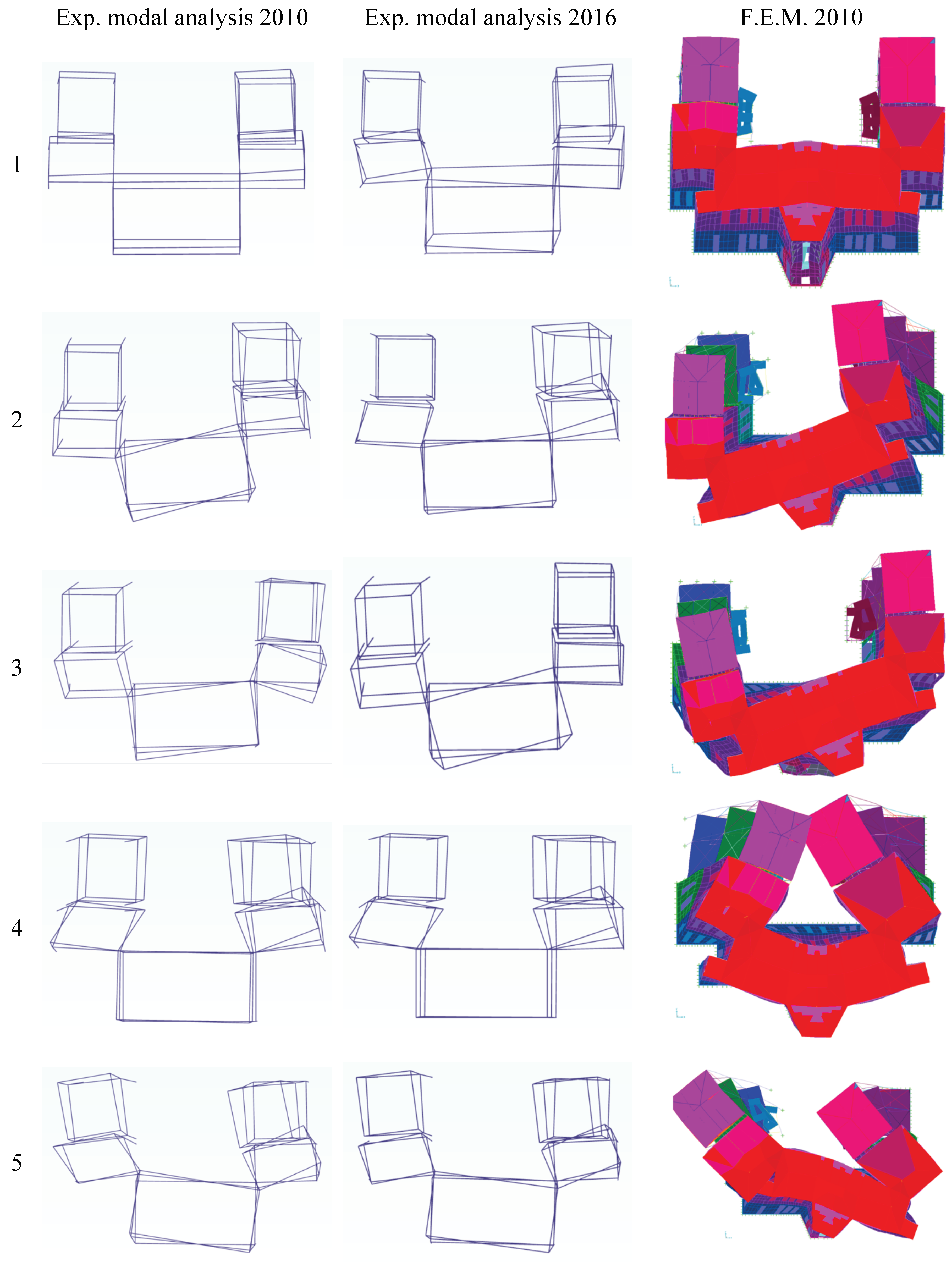
With the aim of allowing a clear depiction of modal shapes, the floors have been subdivided in 5 rectangular portions: the displacement of a generic point has been calculated by those of the instrumented points imposing rigid body constraints on each portion.
Table 1 collects the natural frequencies obtained by both 2010 and 2016 data sets, while in
Figure 5, the corresponding modal shapes are depicted. The first 4 frequencies fall in a narrow frequency range (6.03–6.94 Hz). Starting from the 2010 data set, as expected, the first mode is mainly in the Y direction, while the second mode is mainly torsional. In the third mode, the main portion of building C exhibits a torsion: one wing and one RC building accomodate it, while the other parts oppose it. In the fourth mode, the main wing of building C exhibit a small translation in X, while both wings translate and rotate in opposite directions. In the fifth mode, the main wing of building C exhibits a torsion, while the secondary wings of building C and both buildings A and B oppose it. Comparing the behaviour of the structural joints near buildings A and B, it is evident that, despite a significant coupling of all buildings, building B is more independent with respect to building A.
Using the 2016 data set, a slightly different dynamical behaviour can be observed. The natural frequency of the first mode does not change; for the second to fourth mode, 3–5% increments are observed, while the fifth mode exhibit a 1% reduction. The frequency increment can be reasonably explained considering a slight increment of the stiffness of buildings A and B, where the infill walls and the partitions were covered by a reinforced plaster during the 2012 interventions. The deformed shapes are generally similar to that of the 2010 dataset, but the second mode of 2016 resembles the third mode of 2010 and vice versa. Concerning the behaviour of structural joints near buildings A and B, it is confirmed that there is a significant coupling of all buildings and an independence of building B, but also, building A appears slightly more independent with respect to the 2010 configuration, especially with reference to the first mode shape. This behaviour can be attributed to the 2012 interventions, when the joint dimensions have been verified.
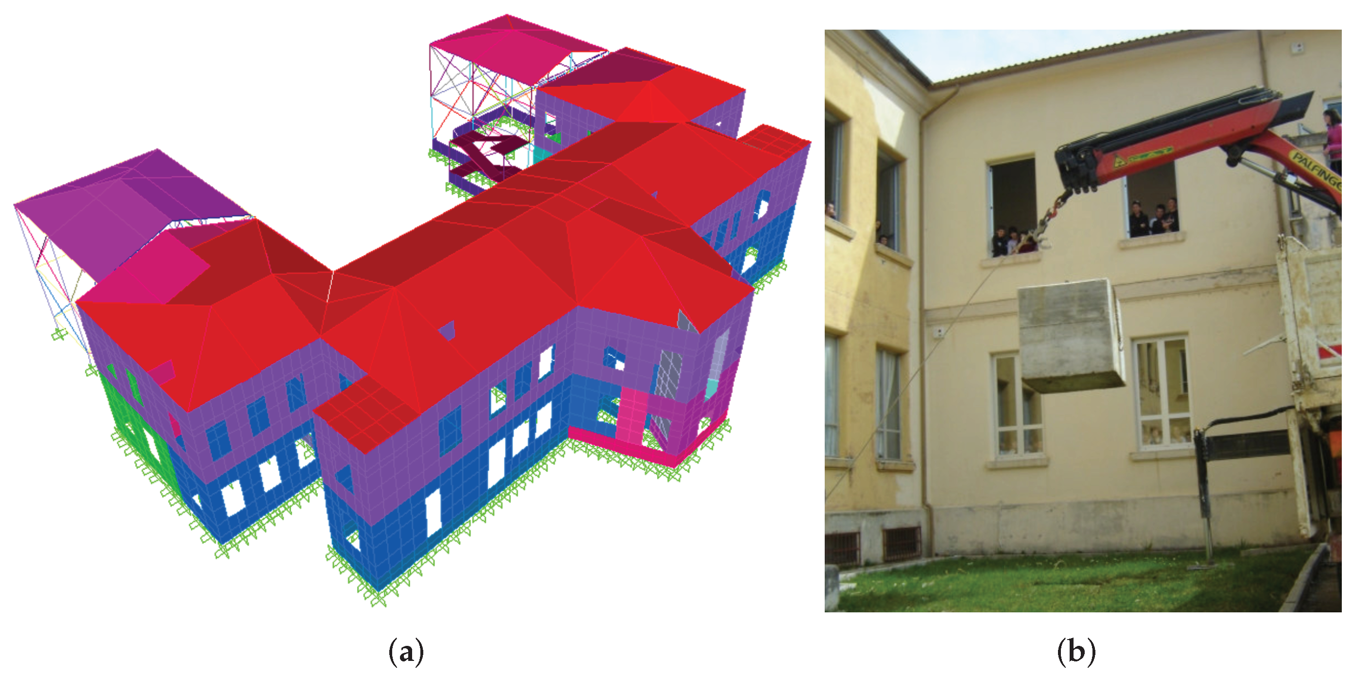
Like all other structures belonging to OSS, for this aggregate, a FEM has been developed in 2011 (
Figure 6a) using a commercial software [
27]. The a priori model characteristics were based on the geometry and material properties purposely investigated after the installation of the monitoring system; then, the parameters of the a priori model were updated to reasonably match experimental frequencies and mode shapes obtained by small vibrations induced on the structure by letting a RC block fall on the ground near the building at the monitoring system installation time (
Figure 6b).
Taking into account that the aggregate of buildings C, A and B, at least at small level sof vibration, exhibit a dynamical behaviour as a whole, a global model has been created (
Figure 6a). The masonry walls of building C and the slabs have been modelled using shell elements; the columns and beams of buildings A and B and the roof trusses have been modelled using frame elements, while the corresponding plane elements in
Figure 6a were used only to simulate the masses. The infilled walls of buildings A and B have been modelled using equivalent diagonal struts. For the external underground walls, the soil-structure interaction has been modelled using equivalent horizontal springs. The nodes of the model have been considered fixed at the base.
Firstly, a brief description of the a priori model is given. The dead weight of the slabs are reported in the following: inclined slabs with deformed steel sheets, 170 kg/m2; stairs, 500–700 kg/m2; RC floor slabs, 450–550 kg/m2; horizontal RC slabs under the roof and inclined RC slabs of the roof, 300–350 kg/m2, which leads to significant masses at the top. For the masonry walls, the unit weight was assumed to be 2200 kg/m3; for hollow clay walls, the unit weight was assumed to be 700 kg/m3; and for RC elements the unit weight was assumed to be 2200–2500 kg/m3 (depending on in situ tests). The elastic modulus was assumed as follows: RC columns, 21,000–28,000 MPa (a 0.8 reduction coefficient with respect to test values was applied to take into account the cracked properties); RC beams, 13,000–17,000 MPa (0.5 reduction coefficient for cracked properties); masonry, 2300 MPa. For infilled walls, an equivalent elastic modulus of 7900 MPa was initially set, and the transversal dimension of the equivalent strut was set to 20% of the diagonal length. In the a priori model, the structural joints were considered not effective (continuity between buildings A, B and C).
The calibration of the model, based on the minimization of the error between experimental and numerical frequencies and mode shapes, leads to the following updated parameters: the elastic modulus of the masonry was set to 1600 MPa (30% reduction); the elastic modulus of the infills of building A was increased by 10%, while that of building B was reduced by 25%; furthermore, the joints were considered effective only for building B at all floors, except at the roof level. In the framework of structural identification procedures, model updating techniques usually involves suitable analytical nonlinear procedures to drive the optimum selection of the parameters [
28,
29]. When the focus of the study, like in the present case, is on the analysis of the seismic performance, rather than on the analytical features of the method, a linearized modified procedure based on [
30] can be effectively applied.
The results in terms of natural frequencies are reported in
Table 1 under the column FEM2010. The error is generally very small, between 0 and 1%; only for the fourth mode is the error 2.2%. The mean error is 0.62%. The comparison in terms of mode shapes is reported in
Figure 5, and results are very satisfactory; due to visualization approximations, buildings C and B seem connected at all floors, but in the model, they are connected only at the roof level. The modal participation masses of this model are reported in
Table 2: a good agreement can be observed with respect to the description of the experimental modal shapes reported in
Table 1.
With the aim to confirm the confidence in the global model of the aggregate, single models of each building are examined: they are not able to reproduce the experimental behaviour. In
Table 3, the dynamical properties of the independent models are reported. The experimental frequencies are poorly approximated by separate models, while they are in good agreement with the global model FEM2010 of
Table 1. It appears that the C building mainly influences the behaviour of the aggregate. The experimental first mode can be interpreted as the effect of the connection of new buildings A and B to the old building C; the resulting experimental frequency (6.03 Hz) falls in the range of the first frequencies in the Y direction of the separate models (5.78, 6.81, 7.01).
As already discussed, in 2012, some structural interventions were made. Thus, the FEM2010 model has been modified in order to approximate the new dynamical parameters reported in
Table 1 under the column “Experimental 2016”. The new model, called FEM2016, reflects those structural modifications involved deletion of the connections between buildings A and C at all floors, except at the roof, analogous to building B in the FEM2010 model and a 10% increment to the elastic modulus of the masonry infills due to the reinforced plaster applied to the walls.
The results obtained in terms of natural frequencies are reported in
Table 1 in the corresponding column. For FEM2016, the error is generally very small, between 0.3 and 1.7%. Only for the second mode is the error 4.2%; in this case, the mean error is 1.22%, greater than the 0.62% mean error obtained with FEM2010. The modal shapes obtained with model FEM2016 are not reported, because they are very similar to those of FEM2010 in
Figure 5.
Different from the experimental results where, as already observed, there is an exchange between the second and third modes of the 2010 and 2016 measurements, this is not present in the numerical shapes. In any case, the result obtained was considered sufficiently approximate to use this model for the kind of simulations discussed in the following section.
5. Experimental and Numerical Analysis of the 2016 Earthquake Response
The 2016 earthquake was recorded by the OSS monitoring system, and several types of information can be gathered based on both the strong motion characteristics and on the building response.
5.1. The Recorded Strong Motion
A detailed analysis of the signal recorded at the base level (position NF of
Figure 4) is outside the scope of this paper. Few data can be discussed in order to put the aggregate behaviour in the larger picture of the effects of the earthquake on the territory.
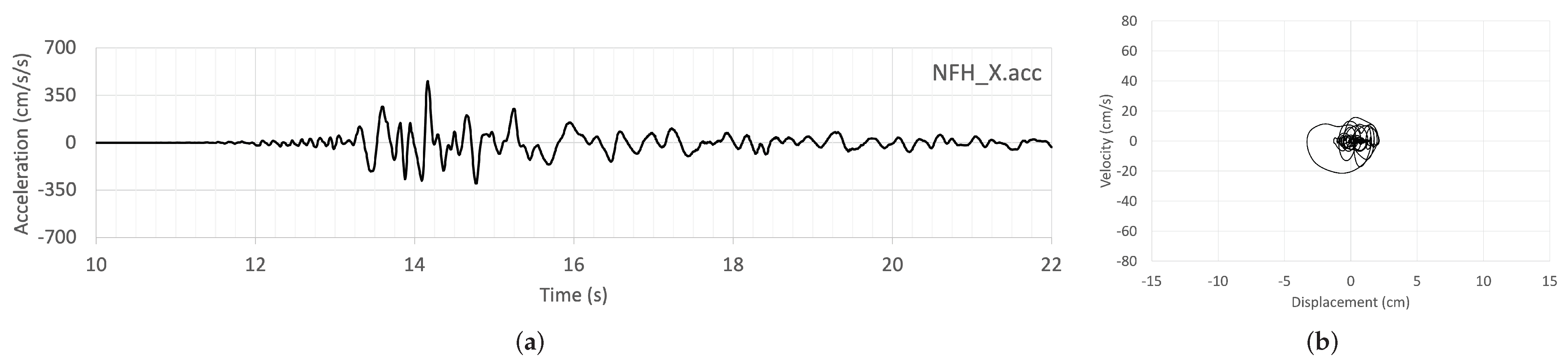
Figure 7 shows the acceleration time history at the base of the aggregate: the peak values are about 0.45, 0.65 and 0.5 g in the
X,
Y and
Z directions, respectively. The prevalent horizontal direction of the base motion was in the
Y direction, as depicted in
Figure 7d, where a single relevant cycle of about 13 cm maximum displacement is evident. This horizontal displacement was coupled to a significant maximum vertical displacement of about 6 cm. Prior to the integration, to obtain velocity and displacement, the acceleration has been processed using a high-pass filter with a 0.25 Hz corner frequency. Using a more sophisticate processing procedure [
31], permanent displacements could be evidenced, but for the aims of this paper, the trajectories reported in the diagrams maintain their validity.
It is also interesting to compare the NF record (in the following called AMTS) with the signal recorded by the RAN station called AMT. RAN is the acronym of Italian accelerometric network, which consists of more than 500 stations. The position of the AMT station is reported in
Figure 1a; the distance between AMT and AMTS is about 800 m, and the difference in elevation is about 80 m (AMTS is the highest). The characteristics of the soil corresponding to AMT and AMTS positions are rather different: the AMTS location can be considered more prone to significant local amplification effects with respect to AMT.
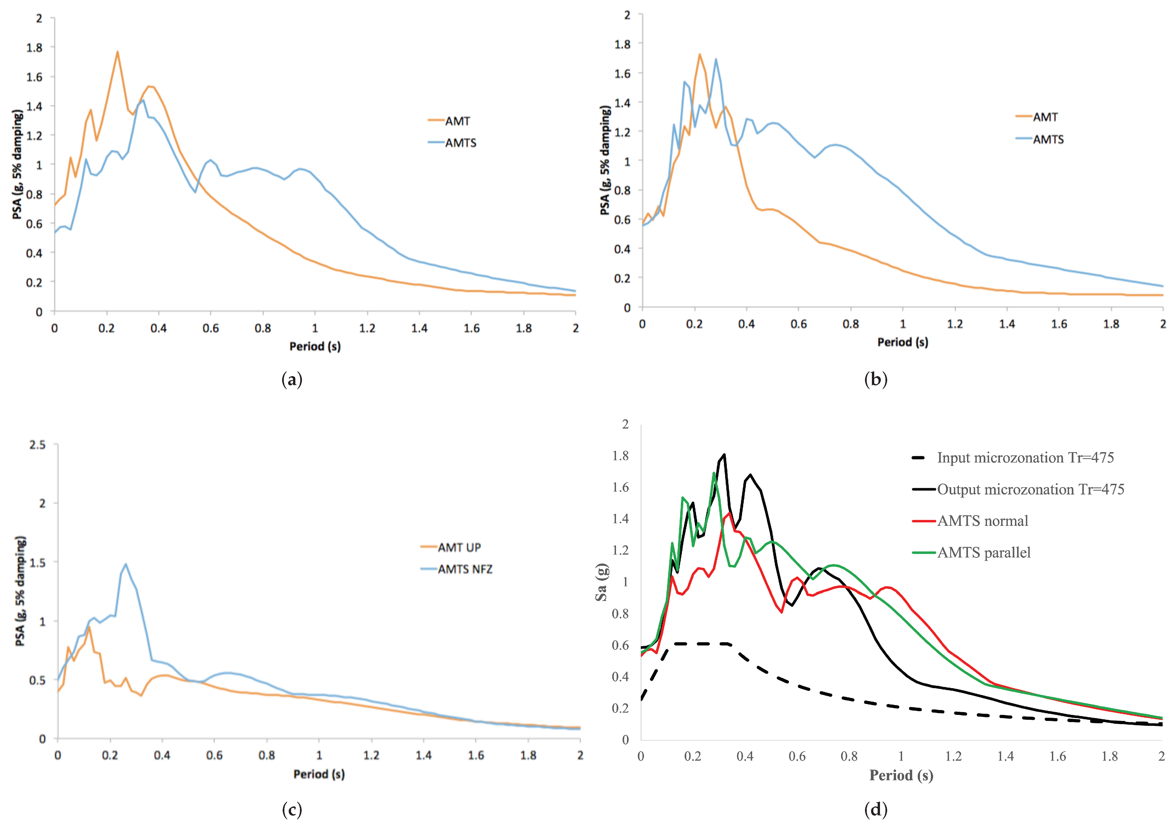
Figure 8a–c allows us to compare the spectral content of the accelerometric records of AMTS and AMT. To make the comparison more consistent from a seismological point of view, the components have been projected with respect to the fault, which is the intersection of the ideal plane representing the earthquake source and the surface of the ground. The usefulness of this projection also stems from the fact that the 2016 earthquake resulted significantly affected by near-source effects: usually these effects influence the parallel component differently from the orthogonal one [
32]. The horizontal spectra are rather similar in the period range between 0 and 0.4 s; for periods greater than 0.4 s, AMTS is more severe. Peak ground acceleration is in the range 0.6–0.8 g; the maximum spectral ordinate is about 1.8 g.
Figure 8d shows that the 475-year return period site amplification spectrum [
33] (output microzonation) is much greater than that on stiff soil (input microzonation). Moreover, the experimental response spectra (AMTS) results are greater than the 475-year spectrum (output microzonation) for the high period range. Thus, it is interesting to evaluate the corresponding return period of this spectra. To this aim, using the information produced by the microzonation program, a spectral amplification curve can be obtained for the AMTS site. Dividing each spectral ordinate of AMTS spectrum by the amplification curve, the site amplification effects are eliminated from the record, and the resulting spectrum can be considered on stiff or reference site. At this point, several response spectra, characterized by various return periods, can be calculated with the formula reported in [
26]; the spectrum with the best approximation furnishes the wanted return period. To reduce the influence of the near fault effects that are not taken into account in the code [
26], it is more suitable to use the parallel component (green curve in
Figure 8d), which, as it can be easily verified, is not significantly affected by this phenomenon. At the end, a return period of 700 years was estimated. For the new school buildings in Italy, the live safety performance is required for a 712-year return period. Usually, for existing buildings, the same performance of a new building cannot be expected if a seismic retrofit has not been performed. In the case at hand, as already written, for building C, a seismic reliability factor of 0.4–0.6 was estimated; by simple calculations, this means that the life safety target fulfilment was expected for an earthquake having a mean return period between 80 and 200 years. Thus, the 2016 earthquake, characterized by a 700-years return period, exceeded that corresponding to the life safety performance.
5.2. The Structural Response
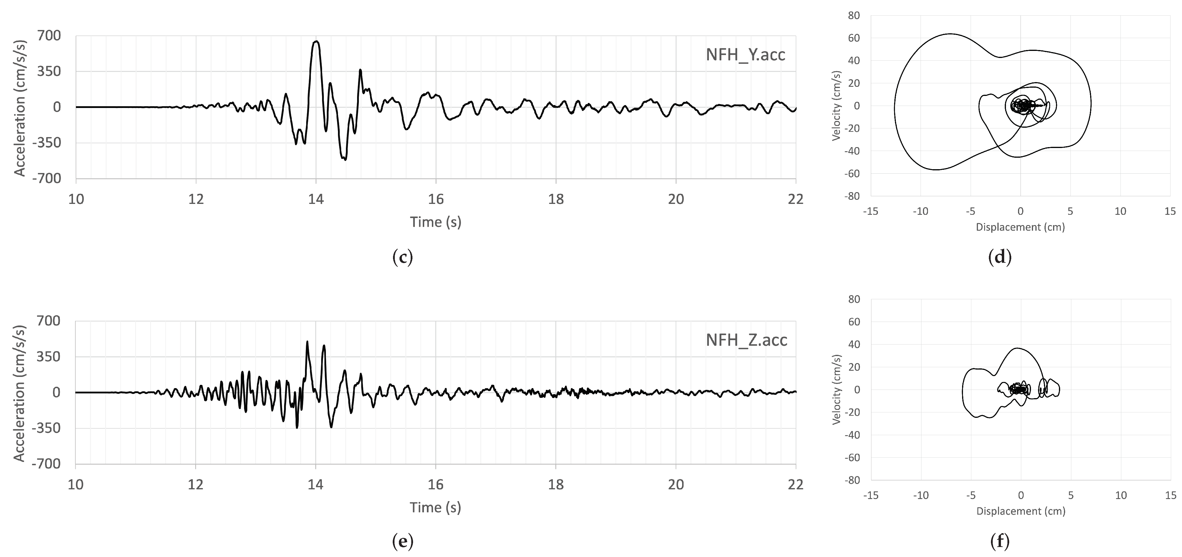
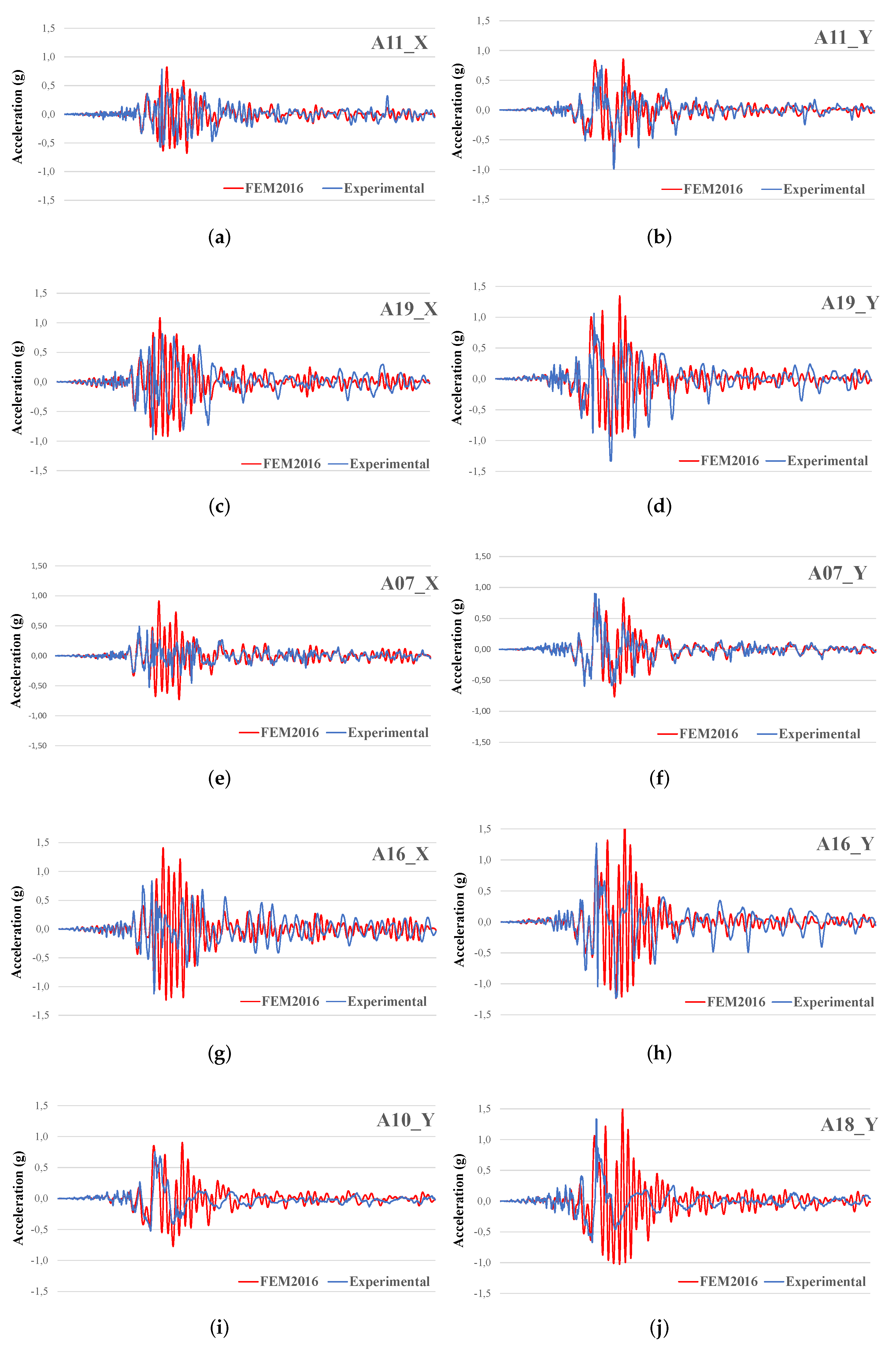
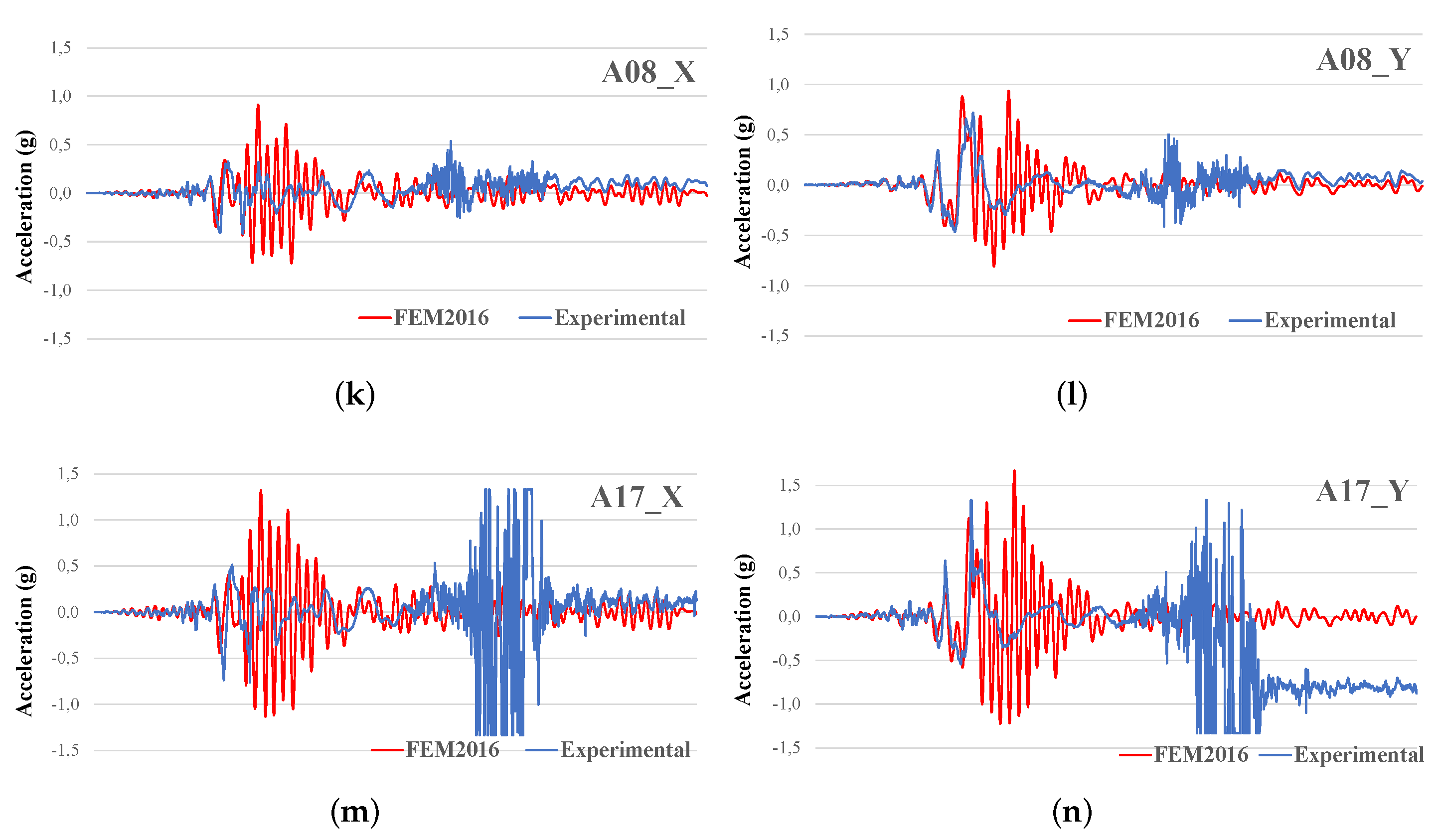
With reference to the performance of the aggregate,
Figure 9 reports acceleration time histories recorded in some points during the 2016 earthquake. In the same figure, the simulations performed with the previously updated FEM2016 linear model are also depicted. As expected [
12,
13,
14,
15,
16,
17,
18,
19,
20,
21,
34], the FEM2016 model is able to reproduce the real behaviour until the elastic limit is exceeded. After that, a significant period of elongation of the structure is evident in the experimental results. Nonetheless, the elastic model is capable of predicting rather well the maximum accelerations at various locations (
Table 4). Obviously, for the portions of the structure affected by a collapse, this comparison is not significant. In any case, the mean error in terms of accelerations results are 7.6% at level 1, 12.9% at level 2 and 15.7% at level 3. This result seems rather interesting, considering the huge nonlinearity experienced by this structure.
As is well known, the damage state of the structural vertical elements, both masonry and RC, can be correlated to the maximum inter-storey drift.
Table 5 lists these values for each building. Even not considering the sensors located in the collapsed portion, very high values of about 3% were attained at the first inter-storey above ground of building C; as a reference, the code [
26] for masonry buildings suggests, for the life safety limit state, maximum values of 0.4% for shear and 0.6% for flexure. The recorded values are indicative that the masonry panels at the second inter-storey attained the collapse limit. The maximum recorded drift at the third inter-storey (between levels 2 and 3) was 0.8%, close to the above-reported range for the life safety performance. At both inter-storeys, the observed damage agreed with that expected according to the code.
For RC buildings A and B, the maximum inter-storey drift was 1.1%. According to the literature [
35] the drift at yielding could be assumed to be about 0.9%, while the drift value corresponding to the near collapse limit state can be assumed to be about 2.3%. The recorded value suggests that the columns exceeded the elastic range, but with limited excursion into the plastic range. This result agrees with the observed damage.
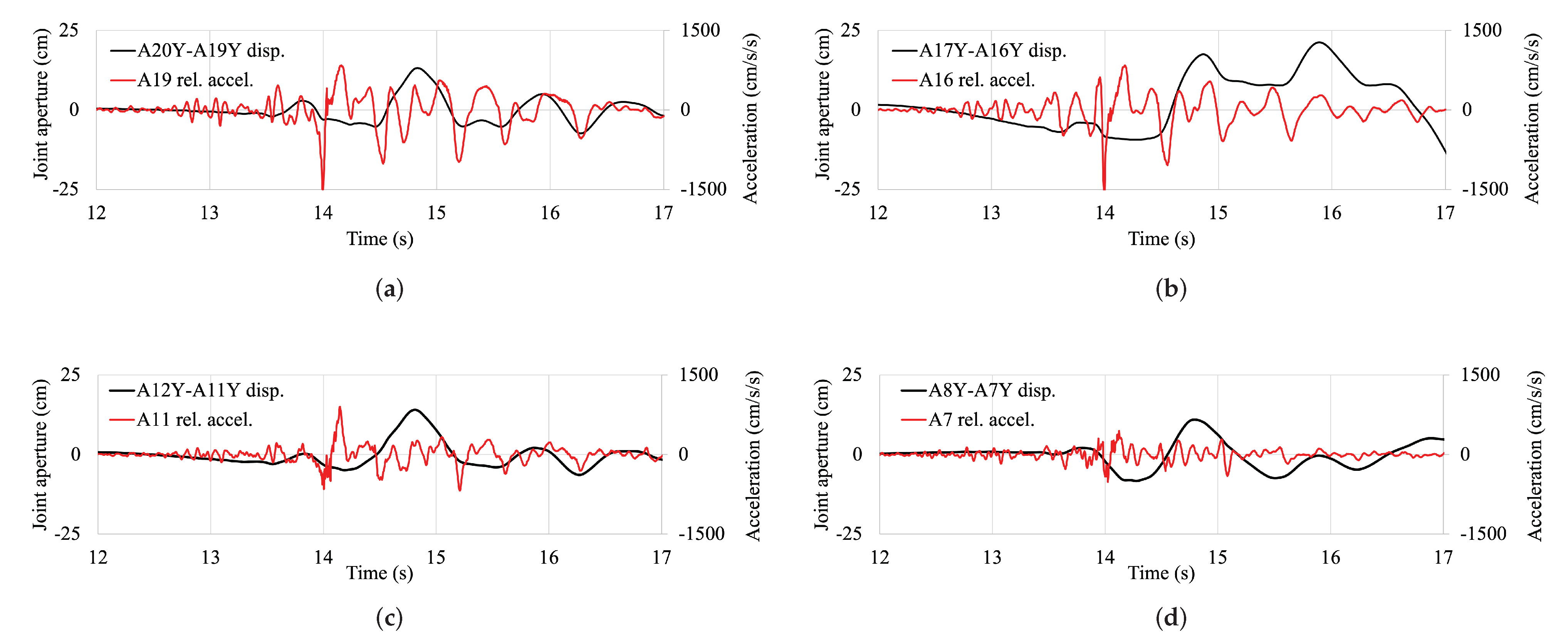
A special attention, for this aggregate, must be paid to the behaviour of the structural joints. The recorded opening of the joints at each level is reported in
Figure 10. At first glance, the relative displacement curves are not symmetric: the closure is always smaller than the opening. Very high values of opening before the collapse of about 15–20 cm were registered. During the first relevant cycle, all joints tend to close and, especially at the roof level, acceleration impulses can be observed, reasonably due to the rupture of the light structures supporting the tiles. The results suggest that the minimum joint dimension, as enforced by the current Italian code, should be improved if pounding between adjacent buildings is judged to be avoided even under very severe earthquakes.
5.3. Evaluation of Local Damage Using Nonlinear Models
A combined experimental-numerical approach has been applied to evaluate local damage in the structure. The procedure is discussed by referring to building A. Nonlinear models of RC buildings have been developed according to the lumped plasticity approach for the monodimensional elements, beams and columns using the “hinge properties” definition of the code [
27]. This nonlinear model does hot have a predictive aim in order to simulate the failure behaviour, but its aim is the use of measured response for the estimation of local damage quantities. The elastic characteristics of the elements were obtained from the linear model of the whole aggregate, previously updated using experimental modal data. For the nonlinear characteristics of the elements, taking into account only the flexural behaviour of the plastic hinges, the yielding
and ultimate
chord rotations and the plastic hinge length
were calculated in accordance to the code [
26]:
where
and
are the yielding and ultimate curvatures of the end sections,
h is the section height,
is the mean diameter of the reinforcements,
and
(in MPa) are the concrete compression strength and steel yielding stress, respectively,
is the shear length, i.e., the ratio between flexural moment and shear (usually assumed equal to one half of the inter-storey height), and
is the seismic action resistant elements. Moreover, the definition of the plastic hinges requires the evaluation of yielding
and ultimate
moments, which are determined under the simplified assumption of constant axial force. Material strength values have been obtained during the already reported survey, performed after the installation of the monitoring system.
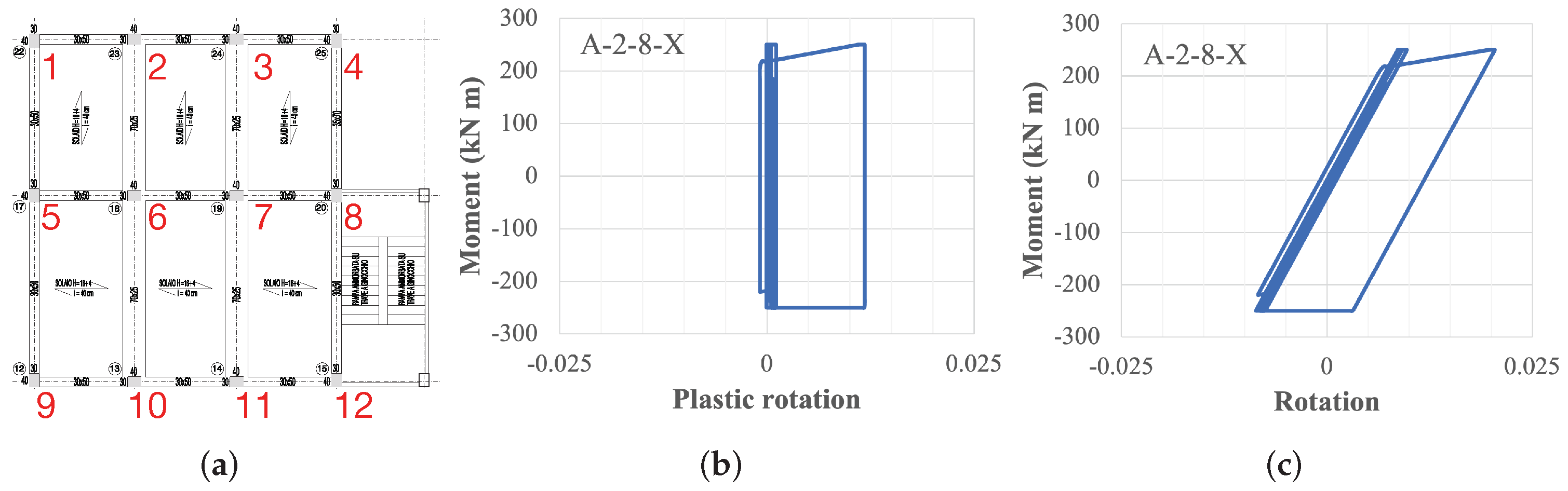
A deformed configuration of the structure is determined on the basis of the displacement time histories recorded during the 2016 earthquake, and the deformation field of each column (
Figure 11a) is estimated as well. To this aim, the recorded displacements were applied to the points of the model corresponding to the location of the sensors; the plane stiffness of the floor slabs allowed us to transfer these displacements to the remaining points. It can be easily recognized that this procedure does not require the knowledge of the nonlinear interaction between buildings C and B. An example of the moment-plastic rotation diagram is reported in
Figure 11b; in
Figure 11c the moment-total rotation is reported. To characterize the local damage
in each element, the following quantity has been calculated:
Obviously, the damage index
is not intended to accurately characterize each possible failure mode (flexural, shear, bond slip, joint failure) of the RC elements: its aim is rather to determine elements more heavily damaged with respect to the others. The values of local rotations and damage are listed in
Table 6. At first glance, the excursion in the nonlinear range was significantly larger for a global displacement of the structure in the Y direction, confirming the results of
Table 5. Moreover, the values of
were greater at the base level than at the upper floor. It is well known that damage indices are generally affected by a high degree of scatter [
36]; thus, in this case,
can be especially useful to compare the state of damage of different columns. With this in mind, the damage level was generally moderate, with the exception of two columns, 8 and 12, adjacent to the external stairs at the second inter-storey, were
was very high. This quantitative damage estimation was confirmed by a direct inspection after the earthquake; in particular, the conditions of the most damaged columns of building A can be observed in the last image of
Figure 2.
While the inter-storey drift values calculated directly from the measures (
Table 5) represent a mean value along a vertical alignment, the local chord rotation values calculated using the nonlinear model (
Table 6) highlight the peaks of damage to the most stressed parts of the structure. For example, column A-12 attained a maximum chord rotation of 1.98% at inter-storey 2 at the upper plastic hinge, to be compared to the mean inter-storey drifts of 1.1% of sensor A11Y of
Table 5.
6. Conclusions
A school building aggregate, equipped with a permanent seismic monitoring system by DPC and heavily impacted by the 24 August 2016 Central Italy earthquake was studied. The building aggregate was located in Amatrice and was composed of one masonry and two RC buildings. The main masonry building C was separated by the RC buildings, A and B, through structural joints. Building C underwent a partial collapse, while buildings A and B showed moderate damage, with few localized heavy damaged beam-column joints.
From the signal recorded at the base level of the structure, the acceleration peak value was about 0.65 g, and the prevalent horizontal component of the base motion was in the North-South direction, where a single relevant cycle of about 13 cm maximum displacement was highlighted. The comparison of this recorded motion to that of a different station in Amatrice outskirts, belonging to the national accelerometric network, showed a significant local amplification effect. Indeed, a very good agreement between the experimental response spectra and that derived by a microzonation study was observed. The acceleration response spectra recorded at the base of the building corresponded to a mean return period of about 700 years, similar to 712 years, corresponding to the life safety limit state at present required in Italy for new school buildings. In the case at hand, the seismic vulnerability of the school building was greater than that of a new building, and the same limit state corresponded to an earthquake with a mean return period between 80 and 200 years.
The dynamical properties of the buildings before the 2016 earthquake were obtained from experimental modal analyses. Two configurations of the aggregate were considered: before (called 2010) and after (called 2016) structural interventions performed in 2012. In both results, the first 4 frequencies fell in a narrow frequency range (6.03–6.94) Hz, and, despite the presence of structural joints, a significant coupling of all buildings was registered. Using the 2016 data, a slight increment of frequencies was observed due to the reinforcement interventions, and a small modification of the mode shapes was observed as well, probably related to the upgrading of structural joints between B and C and A and C buildings.
An FEM was developed on the basis of geometric and material properties purposely investigated. Then, model parameters were updated to reasonably match the experimental frequencies and mode shapes obtained by small vibration tests. The aggregate exhibited a dynamical behaviour as a whole, and a global model was created accordingly. The results of the FEM in terms of natural frequencies and mode shapes were very satisfactory, and the updated model was used in the simulation of the response to the 2016 earthquake.
This updated FEM was subjected to the base excitation recorded during the 24 August 2016 earthquake. As expected, the model is able to reproduce the real behaviour fairly faithfully until the elastic limit is exceeded. After that, a significant period of elongation in the experimental structure response is evident. It is worth noticing that the maximum accelerations at various locations predicted using the elastic model are in good agreement with the measured values: the mean error was between 7.6% and 15.7% at the first and third building level, respectively. This result seems rather interesting considering the huge nonlinearity experienced by this structure, and suggests the need to study more in depth the capability of linear models to predict the structural response in terms of acceleration and probably in terms of force.
A special attention has been paid to the behaviour of the structural joints. It can be observed that the relative displacement curves are not symmetric: the closure is always smaller than the opening, which reached high values of about 15–20 cm, greater than the gap required by the current seismic code. This result suggests that this minimum joint dimension should be improved if pounding between adjacent buildings is deemed to also be avoided under severe earthquakes.
Nonlinear models of RC buildings have been developed from the linear model of the whole aggregate. The beams and the columns were modelled according to the lumped plasticity approach: plastic hinges were defined at each beam-column joint. The recorded displacement time histories were applied to the nodes of the model of building A, and the deformation of the elements were determined. Thus, a local damage in each element was calculated, and a damage index was introduced, which made it possible to describe the different conditions of the structural elements.
As expected, the excursion in the nonlinear range was significantly larger for a deformed configuration of the structure in the North-South direction, where the earthquake component is stronger. In any case, the damage level generally was moderate, with the exception of two columns adjacent to the external stairs, where the index reached the highest values. This quantitative damage estimation was confirmed by a direct inspection after the earthquake. While the inter-storey drift values calculated directly from the measured quantities represent a mean value along a vertical alignment, the combined use of a nonlinear model allows for highlighting the peaks of damage in the most stressed elements of the structure.
In a SHM perspective, in this paper, the use of experimental results and nonlinear models has been combined: in particular, a numerical model has been used along with experimental results to obtain information at a local level, thus allowing the estimation of damage on all relevant structural elements. This technique can be very useful in general to obtain more significant results from recorded responses.


