Shaking Table Seismic Experimental Investigation of Lightweight Rigid Bodies

Abstract

This study presents the findings of an extensive shaking table experimental campaign conducted on nine free-standing wooden specimens, aiming at providing insights on the rigid body motion of free-standing objects. The specimens, which differ in slenderness and size, are characterized by impairments in their base surface and most likely in their shapes, which also lead to asymmetric responses. The imperfections of the tested objects are an additional source of uncertainty with respect to the intrinsic chaotic character of the rigid body motion, which is a crucial factor that prevents the reproducibility of the tests and induces discrepancies between specimen responses and those of their ideal models. A contactless measurement strategy is employed to assure unaltered data acquisition. The experimental campaign includes free vibration tests, pulse excitation, and natural ground motions tests; the dynamic responses of the specimens are organized and rearranged, aiming at providing a comprehensive set of data that could be employed for calibrating numerical models accounting for imperfect conditions. The damping properties of the specimens are discussed, providing a novel estimation of the coefficient of restitution based on the free vibration tests. The limits of the ideal simple rigid model are highlighted, and the roles of size factor and aspect ratio are discussed according to the obtained results.

1. Introduction

Rigid body motion can describe a wide variety of structural systems both in the field of civil engineering [1,2,3] and in the protection of ancient remains [4,5,6] and artworks [7,8,9,10], especially in seismic conditions. In view of the practical implications of the understanding of such systems, starting from the pioneering Housner’s study [11] presented in 1963, the rigid motion of rocking blocks was addressed by several experimental studies that aimed to refine the numerical prediction of their response. Despite the apparent simplicity of these systems, which basically develops through the full contact and the rocking conditions, the intrinsic characteristics of rocking body motion exhibits features that make the full understanding of the physical phenomenon anything but trivial. Rigid body systems are indeed characterized by uplift conditions far from obvious to be identified, by a negative stiffness in the rocking phase, and by an objective difficulty to describe the transition conditions at each impact (usually treated by means of an empirical coefficient of restitution).

Several authors contributed to improve Housner’s model, extending its features by considering asymmetric blocks [12,13], the occurrence of sliding [14], by extending the model to the three-dimensional behavior [15], or by proposing alternative strategy to evaluate the coefficient of restitution [16,17,18,19,20,21], also with reference to experimental evaluations [10,22]. In other cases, alternative numerical models were proposed, considering moment-rotation laws to describe the rocking motion [17,23,24,25,26].

In order to better observe the rigid block motion, the numerical studies were also combined with the improvement of the experimental knowledge of rocking systems [27,28,29]. These studies were oriented to the identification of the role of an elastic foundation on which the blocks may lay [29], or to the assessment of the impact conditions [27,28]; few extensive experimental campaigns were presented to provide a large amount of data for possible comparison with numerical models [30]. The experimental campaigns usually converge in stating the non-repeatability of the experimental tests [31,32], as also testified by the failing of the numerical models to correctly reproduce experimental results [16,28,33,34,35,36,37,38,39]; such a circumstance is mainly due to the negative stiffness of the rigid body systems, which led some authors to classify the rigid body oscillator as a chaotic system [40,41]. More recently, some authors interpreted the non-reproducibility of the experimental dynamic response of rigid body systems through statistical tools [42], leading to a reasonable prediction of their dynamic response.

In this paper, the results of an extensive shaking table experimental campaign conducted on nine wooden prismatic specimens are presented. The specimens were conveniently designed considering different slenderness and size factors. The tests, conducted in the laboratory of the College of Architecture in Syracuse (University of Catania, Italy), aim both to characterize the blocks in terms of uplift and impact conditions and to observe the full nonlinear behavior under horizontal accelerations. Precisely, two different classes of ground motions were applied, namely pulse excitations ranging both in amplitude and angular frequency, and natural accelerograms with increasing Peak Ground Acceleration (PGA). The results were then collected in convenient behavior maps, which were also compared with the simple rocking model proposed by Housner [11], evidencing the non-reproducibility of the tests and the limits of oversimplified numerical models in simulating the experimental response of block affected by impairments. The experimental measures in terms of displacement were evaluated by tracking the motion of several points with a contactless measuring method, making use of a high frequency acquisition camera and tracking motion software. The employment of contactless measurement technique is particularly suited for lightweight systems, where the use of accelerometers might alter the dynamic properties of the system. Alternative contactless strategies were already proposed in the literature, such as the 3D Laser Vibrometry [43], which exploits the Doppler shift of the laser beam reflected off the vibrating surface. The results, which represent a large database of tests at disposal of other researchers [44] for comparison with advanced numerical models, are also an opportunity to discuss the role of slenderness and size factor in the stability of the blocks (Supplementary Materials).

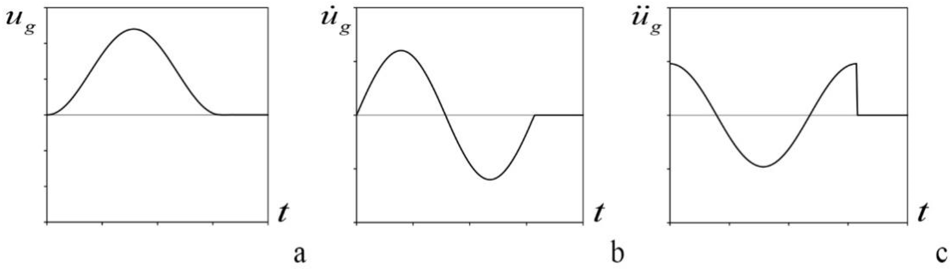
2. Rigid Body Motion

The dynamic behavior of free-standing objects is governed by rigid body motion. Indeed, for such structures the deformability is usually negligible, and the dynamic behavior may be characterized by a full contact phase until the acceleration module reaches an uplift threshold; then the block starts to rock and the collapse for such structural systems is conventionally associated to the overturning of the block. The 2D Simple Rocking Model, depicted in Figure 1, is due to Housner’s pioneering studies [11], and consists of a rigid body representing a generic free-standing object, characterized by a mass $m$ and polar moment of inertia $I_G$ with respect to its center of gravity $G$. In his original work, Housner assumed the body as symmetric and presented the simple case of a homogeneous rectangle. In the latter case, the block has height $2h$ and base $2b$, respectively; in addition, the hypothesis of inhibited sliding at the base of the block was assumed. The dynamics of the model can be described considering as single Lagrangian parameter the rotation $\theta$ of the body, assumed positive if clockwise, i.e., when the right edge of the block is in contact with the base.

The full contact persists until the ground acceleration ${\ddot{u}}_g(t)$ achieves a convenient threshold:

$$\left|{\ddot{u}}_g(t)\right|\le g\hspace{0.33em}b/h$$

(1)

where $g$ is the gravity acceleration. Once the block starts rocking, the governing equation of the dynamics of the system is the following one:

$$\ddot{\theta }(t)=-p^2\left\{\frac{{\ddot{u}}_g}{g}\cos \left[\alpha \mathrm{sgn}\left(\theta (t)\right)-\theta (t)\right]+\sin \left[\alpha \mathrm{sgn}\left(\theta (t)\right)-\theta (t)\right]\right\}$$

(2)

where $\alpha =\arctan \left(h/b\right)$ is a parameter representing the slenderness of the block and $p$ the frequency parameter given by

$$p=\sqrt{\frac{mgd}{I_G+m{d}^2}}=\sqrt{\frac{mgd}{I_o}}$$

(3)

being $d\hspace{0.17em}$ the distance of the edge of the block from the center of gravity, whilst $I_O$ is the polar moment of inertia of the block respect to one of its pivoting edges.

During the rocking phase, impacts ($\theta =0$) can occur at the base of the block and the rotation $\theta (t)$ can change sign. Each impact is characterized by an instantaneous energy loss that reduces the rotation velocity according to a coefficient of restitution $e$ as follows:

$${\dot{\theta }}^{+}=e {\dot{\theta }}^{-}$$

(4)

where ${\dot{\theta }}^{-}$ and ${\dot{\theta }}^{+}$ represent the angular velocities immediately before and after the impact, respectively.

This ideal model is easy to handle but can fail in predicting the actual dynamic behavior of rigid blocks. In order to extend the features of the Simple Rocking Model, it was upgraded considering the possible occurrence of sliding [14], and also accounting for asymmetric [12,13] or three-dimensional behavior [15]. Finally, a considerable number of studies were devoted to analyze and propose realistic approaches for evaluating the coefficient of restitutions [10,22]. It is worth mentioning that no model, even the most advanced one, can get rid of the chaotic character of the rigid body motion, for which there is strong evidence brought to light in some studies [40,41,42].

3. Test Setup

By employing a unidirectional shaking table and making use of a contactless acquisition data strategy, some aspects of the dynamic behavior of several specimens with different aspect ratios and size factors are investigated. The experimental campaign reported herein is part of a wider research conducted within a PhD study on the seismic protection of art objects [45]. In the following subsections, to provide a clear framework of the experimental campaign, the specimens characteristics are first introduced, then the lab equipment and the testing protocol are presented. The results of the experimental campaign and the relevant discussion are finally reported in the next section.

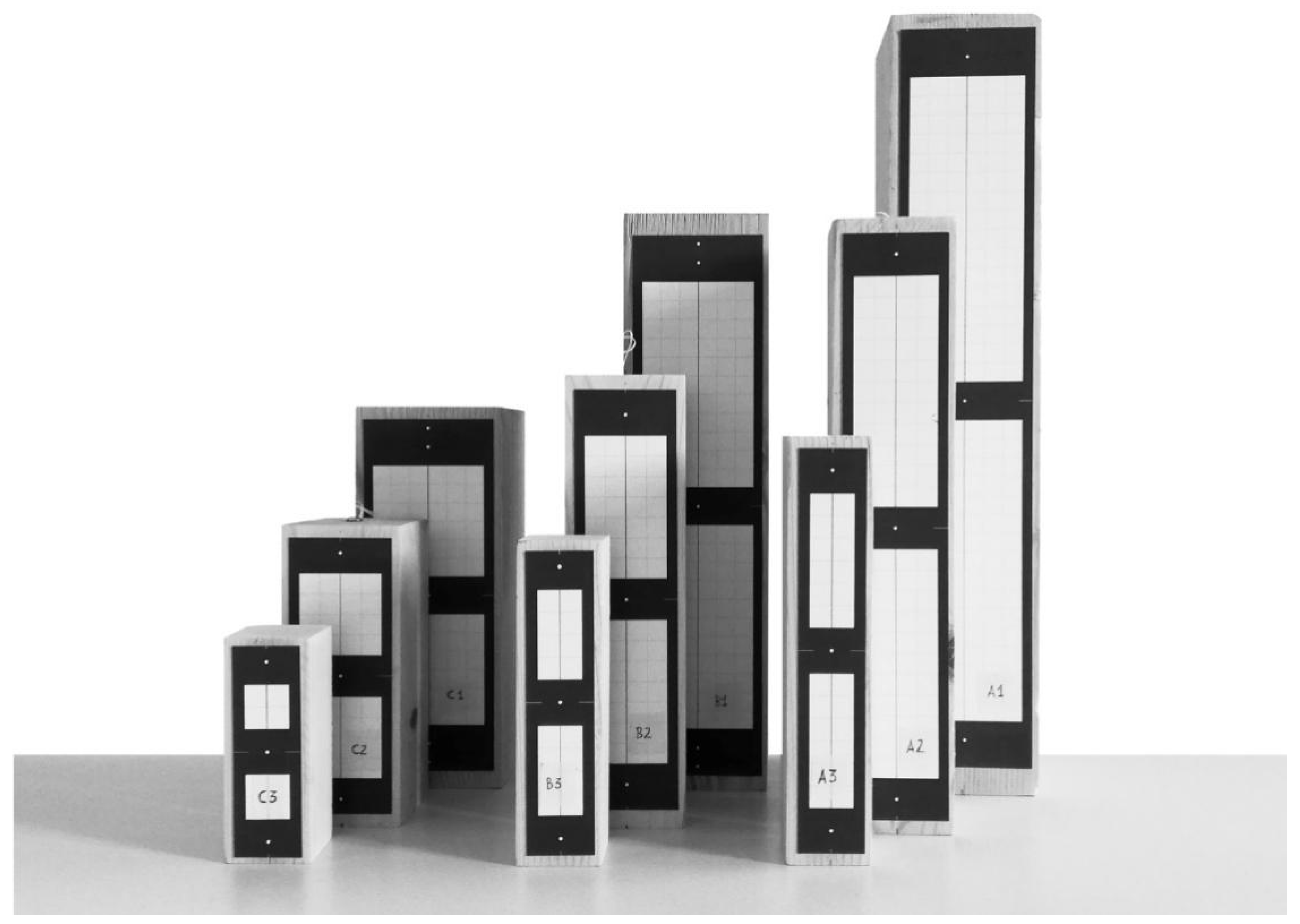
3.1. The Adopted Specimens

Nine wooden specimens were tested, Figure 2, considering three different aspect ratios and three size factors, as better specified in

Table 1. Tested specimens: measured and theoretical parameters. Values (¹) measured on the specimens and values (²) indirectly obtained from theoretical formulation.

	A1	A2	A3	B1	B2	B3	C1	C2	C3
Aspect ratio $\lambda =h/b$	5.2083	4.9883	5.0000	3.8927	3.7811	3.7772	2.5676	2.5133	2.6383
Size factor $d_i/d_1$	1.0000	0.7124	0.4607	1.0000	0.7113	0.4642	1.0000	0.7138	0.4845
m [kg] (1)	1.286	0.435	0.113	0.995	0.300	0.084	0.641	0.201	0.059
b [m] (1)	0.0384	0.0285	0.0184	0.0385	0.0282	0.0184	0.0389	0.0283	0.0184
h [m] (1)	0.2000	0.1423	0.0920	0.1500	0.1065	0.0695	0.0998	0.0710	0.0485
d [m] (2)	0.2037	0.1451	0.0938	0.1549	0.1102	0.0719	0.1070	0.0764	0.0519
δ [rad] (2)	0.1897	0.1978	0.1974	0.2515	0.2586	0.2588	0.3714	0.3787	0.3623
IG [kg m2] (2)	0.017783	0.003049	0.000331	0.007956	0.001213	0.000143	0.002448	0.000390	0.000054
IG + md2 [kg m2] (2)	0.071119	0.012206	0.001326	0.031821	0.004854	0.000577	0.009794	0.001564	0.000213
p [rad/s] (2)	6.0105	7.1221	8.8572	6.8924	8.1728	10.1331	8.2905	9.8157	11.8824

. The specimens are characterized by a very simple shape (parallelepiped), and by an apparent symmetry. The Size factor represents the semi-diagonal $d_i$ of the generic i-th block normalized by the corresponding value $d_1$ of the reference largest block; the slenderness ($\lambda$) is the ratio between the height and the base of the i-th block. The specimens were placed on a sheet of sandpaper, the effectiveness of which for avoid sliding during the tests was experimentally verified.

The characteristics of the specimens are identified by an alphanumeric code in which the letters from A to C define the slenderness that gradually decreases (type A means slender, type C means squat), whereas the numbers from 1 to 3 characterize the size factors of the blocks with gradually smaller dimensions (type 1 is the biggest, type 3 is the smallest). Convenient paper sheets were glued to the front face of the specimens, reporting several markers that were employed for the contactless data acquisition during the tests, as better described in the next subsection.

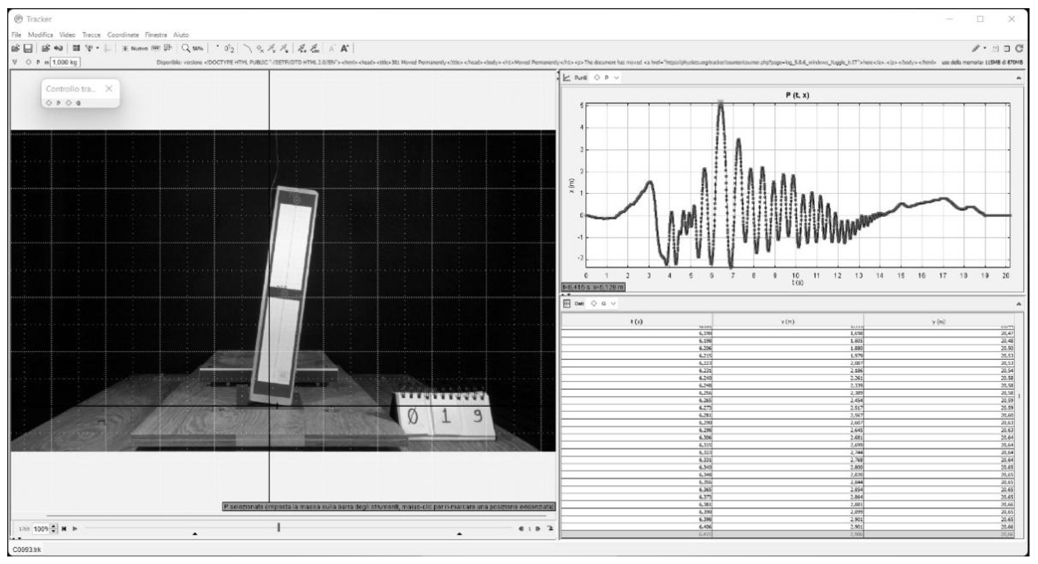
3.2. Instrumentation and Testing Protocol

A contactless displacement data acquisition system was developed for the experimental campaign. Such a strategy implies undoubtful advantages since it does not require additional mass constrained to the specimen, which could interfere during the test by changing the dynamic properties of the system. In addition, the tests are easily repeatable, and no cabling is required. The low frequency content of the problem at hand assures that displacement acquisition is appropriate and accurate, although the data processing for digital image correlation can take a considerable time. In the case of test repetitions, to guarantee a faithful guided repositioning of the block, a traced footprint was emplaced on the shaking table.

As already mentioned, the block response is determined by employing markers whose position can be traced during the tests by means of a high-frequency acquisition camera located on a tripod in front of the shaking table, as shown in Figure 3. Once the video acquisition is completed, the frames are processed using the Tracker Video Analysis and Modelling Tool software ver. 5.0.7 [46], Figure 4.

The ground motion is applied through a unidirectional shaking table designed to perform seismic simulations or vibration tests. The shaking table, from the LO.F.HI.S. series ND13014 (Low Frequency High Stroke and Velocity Shaker) distributed by CENTROTECNICA S.R.L., consists of an aluminum plate forced to move in one direction using the linear motor technology that defines the position of the plate over time. It has a total weight of 6500 N and a working area of 650 × 500 mm to accommodate a maximum payload of 100 kg. The vibrating table, with displacement control, allows a maximum displacement capacity of 28.6 mm (±14.3 mm), maximum speed of 2.5 m/s, and works in a frequency range 0–100 Hz [47].

The displacements of aluminum plate are managed by means of an input. txt file that collects the displacement time histories expressed in micrometers with the desired time step. For this reason, the applied ground acceleration was integrated twice using SeismoSignal software [48].

The Sony DS-RX100 M5 camera used for video records is equipped with a 20.1-megapixel Exmor RS^® CMOS sensor with the ability to record in 4K up to 120 fps, and 1920 × 1080 to 240, 480, and 960 fps in HFR (High Frame Rate) mode.

In particular, the recording was made at 100 FPS (one frame every 0.01 s), setting the focal length to decrease the image distortion at 25.7 mm. The camera is located on a VCT-R640 stand and activated by means of a remote control, Figure 5, which avoids any interference in the initial frames.

The large amount of data is managed with SF-UX2 series SD memory card (Speed Class 10) with high acquisition speed. To improve the lighting conditions, the block was illuminated with three 120 W halogen lamps.

Thanks to the advances in digital photographic tools and the introduction of affordable high-resolution cameras, videogrammetry has been widely used in engineering and applied to the study of the dynamic response of structures. In this context, the two-dimensional (2D) photogrammetry technique was used [49], aiming at reliably measuring the displacement of a limited number of tracking points placed on a planar surface, using a single fixed camera. The adopted method is known as point tracking technique. This approach is based on the identification of the coordinates of discrete points (markers) placed on the structure as optical target (high contrast circular points), Figure 6. The markers layout must be carefully chosen considering that 2D photogrammetry returns reliable results in the case of tracking points positioned in a plane.

A correct acquisition strongly depends on the adopted configuration; to assure a good precision, the camera was located to frame the center of the vertical plane containing the markers with a 90° angle of incidence. In addition, the camera was positioned on stable supports placed outside the shaking table to avoid any vibration interference. Finally, the lighting conditions were also kept as constant as possible. The adopted tracking motion software allows determining the centers of the optical marker using a search algorithm that identifies the optical targets at each instant by comparing them with a reference configuration. The reflecting markers (basically made with a glued paper sheet), which have a very small weight, were placed on the frontal face of the specimens as well as on the shaking table. The latter represents a reference response to be correlated with the outcome of the shaking table, for the calibration phase and to determine measurement accuracy.

The error is evaluated in the post-processing phase when a known real length ($L$ in Figure 7) is related to the corresponding length in pixels.

The accuracy of the measurements was determined by recording the position of a marker at rest over a large time interval [50]. For the adopted configurations, the accuracy of the measurements is about $\pm 0.05$ mm, Figure 8.

A calibration process must be performed to identify the lens alterations. The elimination of barrel distortion can be obtained by realigning the curved lines in the post-processing phase through a procedure that corrects the measurements at the periphery of the frame. The calibration was carried out by choosing a model whose geometry is known and recording the position of some target points constrained to the table and to the object. In particular, the data recorded by the optical reader when the table is pushed to the maximum displacement is used as a reference to correct the measure (Figure 9).

The output of the shaking table can then be compared with that acquired through the acquisition process. It turned out that the correction to be applied is proportional to the distance from the central point of the shaking table; thus, a corrective coefficient can be calibrated to get unbiased data.

Once the procedure is calibrated, the rotation of the block at each step is computed considering the horizontal displacements of vertically aligned markers. Precisely, horizontal displacements were detected and used in the post-processing phase to infer the rotations of the blocks. According to Figure 7, the determination of the rotations for the rigid body was carried out as described below. Two suitable vertically aligned points G and P were chosen in correspondence of the center of gravity and the center top of the rigid body, respectively. Then, as proposed in [10], the rotation can be simply retrieved as:

$${\theta }_i=arcsin\left(\frac{\Delta u_i}{L}\right)$$

(5)

being $\Delta u_i=u_{i,P}-u_{i,G}$ the horizontal relative displacement between the top of the block and the center of gravity for the i-th generic instant. The angular velocity is calculated as follows:

$${\dot{\theta }}_i=\frac{{\theta }_{i+1}-{\theta }_{i-1}}{t_{i+1}-t_{i-1}}$$

(6)

To avoid white noise disturbance of the recording, the quality of the data can be improved after the differentiation with the average method, which consists in calculating the output value $y$ as the average of $k=2N+1$ values $y_k$ (where $k$ is odd) and attributing the calculated value to the central point.

$$y_{N+1}=\frac{{\displaystyle \sum _{k=1}^{2N+1}{y}_k}}{2N+1}$$

(7)

In practice, a very small amplitude window is slid over the signal and replaces a generic value with that derived from the average of the window. The smoothing action of the moving average increases with the width of the considered window. In the data elaboration here presented, $N=3$ was assumed.

4. Experimental Campaign

The section describes the tests, along with the main results. The experimental campaign aims at a complete characterization of the properties and of the dynamic behavior of the blocks. To this purpose, four test typologies were performed, namely two of them search for information on the properties of the blocks; the other two focus on dynamics properties. Specifically, for each of the nine blocks, the performed test typologies are:

• Uniformly accelerated motion to identify the uplift acceleration of the blocks;
• Free rocking oscillations, which aim at experimentally identifying the restitution coefficient;
• Application of pulses with different intensities and angular frequencies, to reconstruct stability maps;
• Ground motions associated to natural accelerograms with increasing PGA.

4.1. Uniformly Accelerated Motion

It is well known that the uplift of a rigid block is associated with the applied horizontal acceleration (in absence of a vertical component), and in particular to a threshold that is theoretically provided by Equation (1). The tests were performed by applying, for each block, a motion of the shaking table corresponding to a uniform acceleration and repeating the test increasing each time the applied acceleration level until the uplift of each block occurred. The identification of such a threshold was obtained by carefully examining the video recording of each test. For each test, the acceleration level was increased considering a step equal to 0.01 g. The obtained results are summarized in

Table 2. Comparison between theoretical (_t) and experimental (_e) uplift accelerations for each block and corresponding reduced uplift coefficient.

A1			A2			A3
${\ddot{u}}_t$ [g]	${\ddot{u}}_e$ [g]	$\alpha$ [-]	${\ddot{u}}_t$ [g]	${\ddot{u}}_e$ [g]	$\alpha$ [-]	${\ddot{u}}_t$ [g]	${\ddot{u}}_e$ [g]	$\alpha$ [-]
0.192	0.120	0.625	0.200	0.140	0.700	0.200	0.130	0.650
B1			B2			B3
${\ddot{u}}_t$ [g]	${\ddot{u}}_e$ [g]	$\alpha$ [-]	${\ddot{u}}_t$ [g]	${\ddot{u}}_e$ [g]	$\alpha$ [-]	${\ddot{u}}_t$ [g]	${\ddot{u}}_e$ [g]	$\alpha$ [-]
0.257	0.190	0.739	0.264	0.240	0.909	0.265	0.150	0.566
C1			C2			C3
${\ddot{u}}_t$ [g]	${\ddot{u}}_e$ [g]	$\alpha$ [-]	${\ddot{u}}_t$ [g]	${\ddot{u}}_e$ [g]	$\alpha$ [-]	${\ddot{u}}_t$ [g]	${\ddot{u}}_e$ [g]	$\alpha$ [-]
0.389	0.290	0.745	0.398	0.350	0.879	0.379	0.280	0.739

where, for each block, both the theoretical, ${\ddot{u}}_t$, and experimental, ${\ddot{u}}_e$, uplift accelerations are reported together with the ratio $\alpha ={\ddot{u}}_e/{\ddot{u}}_t$.

As expected, the observed experimental uplift acceleration is lower than the theoretical one. This is mainly due to the impairments at the base of the blocks and to the imperfectly sharp edges. The reduction is significant; precisely, the difference is never lower than 8% (block B2), but it also reaches the level of 44% in the case of block B3.

It is worth noting that, except for blocks of type B (block B3 basis was particularly defective leading to $\alpha =0.56$ which is significantly lower than the corresponding values for blocks B1 and B2), in the other cases, namely blocks type A and C, the size factor does not seem to play a significant role on the $\alpha$ parameter. On the other hand, as the slenderness increases (i.e., passing from blocks of type C to A), the parameter $\alpha$ tends to decrease, that is slenderness tends to enhance base impairments, leading to a more pronounced decrease of the uplift acceleration of the block.

Such a discrepancy can play a crucial role in the response of the blocks and on capability for a numerical model to simulate the actual behavior of an object. Indeed, in the case of ground acceleration, onset of motion takes place earlier than expected. As will be shown in the next sections, in some cases it may happen that a numerical model based on the theoretical uplift acceleration predicts the block to maintain the full contact phase, whilst the experimental evidence shows a rocking motion (${\ddot{u}}_e<PGA<{\ddot{u}}_t$).

4.2. Free Vibrations

Free vibration tests were performed by enforcing an initial rotation with zero initial velocity to the block. The examination of the response can provide important information regarding the rocking phase and the behavior of the blocks at each impact. The experimental response for the nine blocks in terms of rotation $\theta \left(t\right)$ is depicted in Figure 10.

Slender blocks show longer oscillating periods and less energy dissipation, since the blocks require more time to retrieve the full contact phase. The tests were further interpretated identifying the peak rotations at each oscillation and the contact velocity at each impact, displaying asymmetric response.

With reference to the free rocking motion tests of Figure 10, the main data of the tests in terms of peak rotations and impact velocity (computed according to Equation (6)) are reported in

Table 3. Summary of the results of the free oscillation test block type A1.

$\mathit{j}$	${\mathit{t}}_{\mathit{p},\mathit{j}}$[s]	$\left|{\mathit{\theta }}_{\mathit{p},\mathit{j}}\right|$[rad]	${\mathit{t}}_{\mathit{i},\mathit{j}}$[g]	$\left|{\dot{\mathit{\theta }}}_{\mathit{i},\mathit{j}}\right| [\mathbf{rad}/\mathbf{s}]$	${\mathit{e}}_{\mathit{c},\mathit{j}}$	${\mathit{T}}_{\mathit{e}\mathit{q},\mathit{j}} \left[\mathbf{s}\right]$	$\mathit{j}$	${\mathit{t}}_{\mathit{p},\mathit{j}} \left[\mathbf{s}\right]$	$\left|{\mathit{\theta }}_{\mathit{p},\mathit{j}}\right| \left[\mathbf{rad}\right]$	${\mathit{t}}_{\mathit{i},\mathit{j}} \left[\mathbf{g}\right]$	$\left|{\dot{\mathit{\theta }}}_{\mathit{i},\mathit{j}}\right| [\mathbf{rad}/\mathbf{s}]$	${\mathit{e}}_{\mathit{c},\mathit{j}}$	${\mathit{T}}_{\mathit{e}\mathit{q},\mathit{j}}\left[\mathbf{s}\right]$
0	0.00	0.0904	0.21	0.8593	0.9843	-	1	0.42	0.0864	0.63	0.8073	0.9718	-
2	0.83	0.0798	1.03	0.7969	0.9781	0.83	3	1.22	0.0752	1.43	0.7977	0.9746	0.80
4	1.61	0.0703	1.79	0.7540	0.9791	0.78	5	1.96	0.0666	2.14	0.7034	0.9706	0.74
6	2.30	0.0618	2.48	0.7434	0.9752	0.69	7	2.63	0.0581	2.79	0.6472	0.9791	0.67
8	2.94	0.0552	3.10	0.6395	0.9698	0.64	9	3.25	0.0513	3.40	0.6135	0.9764	0.62
10	3.54	0.0485	3.69	0.6480	0.9812	0.60	11	3.82	0.0464	3.97	0.6147	-	0.57

,

Table 4. Summary of the results of the free oscillation test block type A2.

$\mathit{j}$	${\mathit{t}}_{\mathit{p},\mathit{j}}$[s]	$\left|{\mathit{\theta }}_{\mathit{p},\mathit{j}}\right|$[rad]	${\mathit{t}}_{\mathit{i},\mathit{j}}$[g]	$\left|{\dot{\mathit{\theta }}}_{\mathit{i},\mathit{j}}\right| [\mathbf{rad}/\mathbf{s}]$	${\mathit{e}}_{\mathit{c},\mathit{j}}$	${\mathit{T}}_{\mathit{e}\mathit{q},\mathit{j}} \left[\mathbf{s}\right]$	$\mathit{j}$	${\mathit{t}}_{\mathit{p},\mathit{j}} \left[\mathbf{s}\right]$	$\left|{\mathit{\theta }}_{\mathit{p},\mathit{j}}\right| \left[\mathbf{rad}\right]$	${\mathit{t}}_{\mathit{i},\mathit{j}} \left[\mathbf{g}\right]$	$\left|{\dot{\mathit{\theta }}}_{\mathit{i},\mathit{j}}\right| [\mathbf{rad}/\mathbf{s}]$	${\mathit{e}}_{\mathit{c},\mathit{j}}$	${\mathit{T}}_{\mathit{e}\mathit{q},\mathit{j}}\left[\mathbf{s}\right]$
0	0	0.0877	0.16	1.0013	0.9905	-	1	0.33	0.0854	0.52	0.9407	0.9618	-
2	0.67	0.0769	0.82	0.9035	0.9802	0.67	3	0.98	0.073	1.13	0.9272	0.9645	0.65
4	1.26	0.0666	1.41	0.8737	0.9823	0.59	5	1.54	0.0637	1.69	0.8787	0.9698	0.56
6	1.81	0.0591	1.94	0.855	0.9779	0.55	7	2.07	0.056	2.2	0.8219	0.9700	0.53
8	2.32	0.0521	2.44	0.7587	0.9716	0.51	9	2.55	0.0487	2.68	0.7263	0.9802	0.48
10	2.79	0.0465	2.89	0.7332	0.9674	0.47	11	3	0.0431	3.12	0.7188	-	0.45

,

Table 5. Summary of the results of the free oscillation test block type A3.

$\mathit{j}$	${\mathit{t}}_{\mathit{p},\mathit{j}}$[s]	$\left|{\mathit{\theta }}_{\mathit{p},\mathit{j}}\right|$[rad]	${\mathit{t}}_{\mathit{i},\mathit{j}}$[g]	$\left|{\dot{\mathit{\theta }}}_{\mathit{i},\mathit{j}}\right| [\mathbf{rad}/\mathbf{s}]$	${\mathit{e}}_{\mathit{c},\mathit{j}}$	${\mathit{T}}_{\mathit{e}\mathit{q},\mathit{j}} \left[\mathbf{s}\right]$	$\mathit{j}$	${\mathit{t}}_{\mathit{p},\mathit{j}} \left[\mathbf{s}\right]$	$\left|{\mathit{\theta }}_{\mathit{p},\mathit{j}}\right| \left[\mathbf{rad}\right]$	${\mathit{t}}_{\mathit{i},\mathit{j}} \left[\mathbf{g}\right]$	$\left|{\dot{\mathit{\theta }}}_{\mathit{i},\mathit{j}}\right| [\mathbf{rad}/\mathbf{s}]$	${\mathit{e}}_{\mathit{c},\mathit{j}}$	${\mathit{T}}_{\mathit{e}\mathit{q},\mathit{j}}\left[\mathbf{s}\right]$
0	0	0.1325	0.19	1.4367	0.9846	-	1	0.39	0.1248	0.58	1.353	0.9185	-
2	0.73	0.0948	0.88	1.2427	0.9989	0.73	3	1.02	0.0945	1.18	1.2003	0.9182	0.63
4	1.29	0.0748	1.42	1.1268	0.9827	0.56	5	1.53	0.0715	1.66	1.0353	0.9198	0.51
6	1.75	0.0581	1.87	0.9569	0.9811	0.46	7	1.96	0.0555	2.07	0.9276	0.9212	0.43
8	2.15	0.0458	2.24	0.8976	0.9638	0.40	9	2.33	0.0421	2.42	0.8002	0.9184	0.37
10	2.49	0.0348	2.57	0.7635	0.9708	0.34	11	2.64	0.0326	2.73	0.6714	-	0.31

,

Table 6. Summary of the results of the free oscillation test block type B1.

$\mathit{j}$	${\mathit{t}}_{\mathit{p},\mathit{j}}$[s]	$\left|{\mathit{\theta }}_{\mathit{p},\mathit{j}}\right|$[rad]	${\mathit{t}}_{\mathit{i},\mathit{j}}$[g]	$\left|{\dot{\mathit{\theta }}}_{\mathit{i},\mathit{j}}\right| [\mathbf{rad}/\mathbf{s}]$	${\mathit{e}}_{\mathit{c},\mathit{j}}$	${\mathit{T}}_{\mathit{e}\mathit{q},\mathit{j}} \left[\mathbf{s}\right]$	$\mathit{j}$	${\mathit{t}}_{\mathit{p},\mathit{j}} \left[\mathbf{s}\right]$	$\left|{\mathit{\theta }}_{\mathit{p},\mathit{j}}\right| \left[\mathbf{rad}\right]$	${\mathit{t}}_{\mathit{i},\mathit{j}} \left[\mathbf{g}\right]$	$\left|{\dot{\mathit{\theta }}}_{\mathit{i},\mathit{j}}\right| [\mathbf{rad}/\mathbf{s}]$	${\mathit{e}}_{\mathit{c},\mathit{j}}$	${\mathit{T}}_{\mathit{e}\mathit{q},\mathit{j}}\left[\mathbf{s}\right]$
0	0	0.0784	0.15	0.9835	0.9407	-	1	0.29	0.0677	0.41	0.9124	0.9105	-
2	0.53	0.0545	0.63	0.7944	0.9443	0.53	3	0.74	0.0479	0.83	0.7117	0.9142	0.45
4	0.94	0.0393	1.02	0.6841	0.9518	0.41	5	1.12	0.0353	1.19	0.5982	0.9124	0.38
6	1.28	0.029	1.35	0.5775	0.9481	0.34	7	1.43	0.0259	1.5	0.5203	0.9173	0.31
8	1.58	0.0216	1.63	0.4678	0.9211	0.30	9	1.71	0.0182	1.76	0.4059	0.8959	0.28
10	1.83	0.0145	1.87	0.3112	0.9231	0.25	11	1.94	0.0123	1.98	0.2843	-	0.23

,

Table 7. Summary of the results of the free oscillation test block type B2.

$\mathit{j}$	${\mathit{t}}_{\mathit{p},\mathit{j}}$[s]	$\left|{\mathit{\theta }}_{\mathit{p},\mathit{j}}\right|$[rad]	${\mathit{t}}_{\mathit{i},\mathit{j}}$[g]	$\left|{\dot{\mathit{\theta }}}_{\mathit{i},\mathit{j}}\right| [\mathbf{rad}/\mathbf{s}]$	${\mathit{e}}_{\mathit{c},\mathit{j}}$	${\mathit{T}}_{\mathit{e}\mathit{q},\mathit{j}} \left[\mathbf{s}\right]$	$\mathit{j}$	${\mathit{t}}_{\mathit{p},\mathit{j}} \left[\mathbf{s}\right]$	$\left|{\mathit{\theta }}_{\mathit{p},\mathit{j}}\right| \left[\mathbf{rad}\right]$	${\mathit{t}}_{\mathit{i},\mathit{j}} \left[\mathbf{g}\right]$	$\left|{\dot{\mathit{\theta }}}_{\mathit{i},\mathit{j}}\right| [\mathbf{rad}/\mathbf{s}]$	${\mathit{e}}_{\mathit{c},\mathit{j}}$	${\mathit{T}}_{\mathit{e}\mathit{q},\mathit{j}}\left[\mathbf{s}\right]$
0	0	0.1798	0.26	1.6884	0.9237	-	1	0.44	0.1358	0.62	1.5231	0.9193	-
2	0.76	0.1067	0.91	1.3955	0.9309	0.76	3	1.03	0.0886	1.17	1.29	0.9158	0.59
4	1.27	0.0715	1.38	1.0935	0.9323	0.51	5	1.48	0.0607	1.58	1.0196	0.9205	0.45
6	1.67	0.0503	1.76	0.9833	0.9336	0.40	7	1.84	0.0432	1.93	0.8717	0.9101	0.36
8	1.99	0.0352	2.07	0.8054	0.9425	0.32	9	2.14	0.031	2.2	0.727	0.8878	0.30
10	2.26	0.0241	2.33	0.6323	0.9448	0.27	11	2.38	0.0214	2.33	0.6323	-	0.24

,

Table 8. Summary of the results of the free oscillation test block type B3.

$\mathit{j}$	${\mathit{t}}_{\mathit{p},\mathit{j}}$[s]	$\left|{\mathit{\theta }}_{\mathit{p},\mathit{j}}\right|$[rad]	${\mathit{t}}_{\mathit{i},\mathit{j}}$[g]	$\left|{\dot{\mathit{\theta }}}_{\mathit{i},\mathit{j}}\right| [\mathbf{rad}/\mathbf{s}]$	${\mathit{e}}_{\mathit{c},\mathit{j}}$	${\mathit{T}}_{\mathit{e}\mathit{q},\mathit{j}} \left[\mathbf{s}\right]$	$\mathit{j}$	${\mathit{t}}_{\mathit{p},\mathit{j}} \left[\mathbf{s}\right]$	$\left|{\mathit{\theta }}_{\mathit{p},\mathit{j}}\right| \left[\mathbf{rad}\right]$	${\mathit{t}}_{\mathit{i},\mathit{j}} \left[\mathbf{g}\right]$	$\left|{\dot{\mathit{\theta }}}_{\mathit{i},\mathit{j}}\right| [\mathbf{rad}/\mathbf{s}]$	${\mathit{e}}_{\mathit{c},\mathit{j}}$	${\mathit{T}}_{\mathit{e}\mathit{q},\mathit{j}}\left[\mathbf{s}\right]$
0	0	0.1151	0.11	1.7023	0.9423	-	1	0.22	0.0981	0.33	1.5776	0.9310	-
2	0.42	0.0819	0.52	1.4691	0.9300	0.42	3	0.61	0.0688	0.69	1.3539	0.9283	0.39
4	0.78	0.0579	0.85	1.1843	0.9388	0.36	5	0.92	0.0502	1	1.0812	0.9345	0.31
6	1.06	0.0432	1.13	1.0629	0.9232	0.28	7	1.18	0.0363	1.25	0.8996	0.9178	0.26
8	1.3	0.0302	1.36	0.7679	0.8396	0.24	9	1.41	0.0209	1.46	0.6776	0.9861	0.23
10	1.5	0.0203	1.56	0.5753	0.7907	0.20	11	1.59	0.0125	1.63	0.4624	-	0.18

,

Table 9. Summary of the results of the free oscillation test block type C1.

$\mathit{j}$	${\mathit{t}}_{\mathit{p},\mathit{j}}$[s]	$\left|{\mathit{\theta }}_{\mathit{p},\mathit{j}}\right|$[rad]	${\mathit{t}}_{\mathit{i},\mathit{j}}$[g]	$\left|{\dot{\mathit{\theta }}}_{\mathit{i},\mathit{j}}\right| [\mathbf{rad}/\mathbf{s}]$	${\mathit{e}}_{\mathit{c},\mathit{j}}$	${\mathit{T}}_{\mathit{e}\mathit{q},\mathit{j}} \left[\mathbf{s}\right]$	$\mathit{j}$	${\mathit{t}}_{\mathit{p},\mathit{j}} \left[\mathbf{s}\right]$	$\left|{\mathit{\theta }}_{\mathit{p},\mathit{j}}\right| \left[\mathbf{rad}\right]$	${\mathit{t}}_{\mathit{i},\mathit{j}} \left[\mathbf{g}\right]$	$\left|{\dot{\mathit{\theta }}}_{\mathit{i},\mathit{j}}\right| [\mathbf{rad}/\mathbf{s}]$	${\mathit{e}}_{\mathit{c},\mathit{j}}$	${\mathit{T}}_{\mathit{e}\mathit{q},\mathit{j}}\left[\mathbf{s}\right]$
0	0	0.1376	0.12	1.8976	0.9209	-	1	0.23	0.1121	0.35	1.7481	0.8965	-
2	0.44	0.0867	0.54	1.5214	0.9171	0.44	3	0.63	0.0713	0.73	1.3545	0.9098	0.40
4	0.79	0.0579	0.88	1.1829	0.9114	0.35	5	0.94	0.0474	1.02	1.0753	0.9023	0.31
6	1.08	0.0381	1.14	0.9543	0.9092	0.29	7	1.19	0.0312	1.25	0.8049	0.8971	0.25
8	1.3	0.0249	1.36	0.7168	0.9013	0.22	9	1.4	0.0201	1.45	0.6131	0.8780	0.21
10	1.48	0.0154	1.53	0.5138	0.8847	0.18	11	1.57	0.012	1.61	0.4376	-	0.17

,

Table 10. Summary of the results of the free oscillation test block type C2.

$\mathit{j}$	${\mathit{t}}_{\mathit{p},\mathit{j}}$[s]	$\left|{\mathit{\theta }}_{\mathit{p},\mathit{j}}\right|$[rad]	${\mathit{t}}_{\mathit{i},\mathit{j}}$[g]	$\left|{\dot{\mathit{\theta }}}_{\mathit{i},\mathit{j}}\right| [\mathbf{rad}/\mathbf{s}]$	${\mathit{e}}_{\mathit{c},\mathit{j}}$	${\mathit{T}}_{\mathit{e}\mathit{q},\mathit{j}} \left[\mathbf{s}\right]$	$\mathit{j}$	${\mathit{t}}_{\mathit{p},\mathit{j}} \left[\mathbf{s}\right]$	$\left|{\mathit{\theta }}_{\mathit{p},\mathit{j}}\right| \left[\mathbf{rad}\right]$	${\mathit{t}}_{\mathit{i},\mathit{j}} \left[\mathbf{g}\right]$	$\left|{\dot{\mathit{\theta }}}_{\mathit{i},\mathit{j}}\right| [\mathbf{rad}/\mathbf{s}]$	${\mathit{e}}_{\mathit{c},\mathit{j}}$	${\mathit{T}}_{\mathit{e}\mathit{q},\mathit{j}}\left[\mathbf{s}\right]$
0	0	0.1602	0.12	2.3119	0.8971	-	1	0.21	0.1212	0.32	1.9921	0.8712	-
2	0.4	0.0875	0.48	1.7293	0.8986	0.40	3	0.55	0.0688	0.63	1.4585	0.8668	0.34
4	0.68	0.0504	0.75	1.2917	0.9108	0.28	5	0.8	0.0413	0.86	1.1194	0.8601	0.25
6	0.9	0.0301	0.96	0.9424	0.9073	0.22	7	0.99	0.0246	1.04	0.7669	0.8354	0.19
8	1.08	0.017	1.12	0.6512	0.8931	0.18	9	1.14	0.0135	1.18	0.4985	0.7773	0.15
10	1.21	0.0081	1.24	0.408	0.9368	0.13	11	1.26	0.0071	1.29	0.3222	-	0.12

and

Table 11. Summary of the results of the free oscillation test block type C3.

$\mathit{j}$	${\mathit{t}}_{\mathit{p},\mathit{j}}$[s]	$\left|{\mathit{\theta }}_{\mathit{p},\mathit{j}}\right|$[rad]	${\mathit{t}}_{\mathit{i},\mathit{j}}$[g]	$\left|{\dot{\mathit{\theta }}}_{\mathit{i},\mathit{j}}\right| [\mathbf{rad}/\mathbf{s}]$	${\mathit{e}}_{\mathit{c},\mathit{j}}$	${\mathit{T}}_{\mathit{e}\mathit{q},\mathit{j}} \left[\mathbf{s}\right]$	$\mathit{j}$	${\mathit{t}}_{\mathit{p},\mathit{j}} \left[\mathbf{s}\right]$	$\left|{\mathit{\theta }}_{\mathit{p},\mathit{j}}\right| \left[\mathbf{rad}\right]$	${\mathit{t}}_{\mathit{i},\mathit{j}} \left[\mathbf{g}\right]$	$\left|{\dot{\mathit{\theta }}}_{\mathit{i},\mathit{j}}\right| [\mathbf{rad}/\mathbf{s}]$	${\mathit{e}}_{\mathit{c},\mathit{j}}$	${\mathit{T}}_{\mathit{e}\mathit{q},\mathit{j}}\left[\mathbf{s}\right]$
0	0	0.2376	0.14	3.2204	0.8800	-	1	0.23	0.1587	0.35	2.8293	0.9210	-
2	0.43	0.1278	0.52	2.4848	0.8833	0.43	3	0.58	0.0946	0.66	2.2565	0.9539	0.35
4	0.73	0.0848	0.79	2.0405	0.8684	0.30	5	0.84	0.0618	0.9	1.8067	0.9798	0.26
6	0.95	0.0591	1.01	1.5097	0.8079	0.22	7	1.04	0.0374	1.09	1.4107	0.9743	0.20
8	1.13	0.0354	1.18	1.1972	0.8096	0.18	9	1.21	0.0228	1.25	1.0137	0.9475	0.17
10	1.28	0.0204	1.33	0.7943	0.7120	0.15	11	1.34	0.0102	1.37	0.5898	-	0.13

for each oscillation. For the generic j-th rocking phase, the instants $t_{p,j}$ corresponding to the peak rotation are registered, together with the subsequent instant of the impact $t_{i,j}$ and the corresponding contact velocity $\left|{\dot{\theta }}_{i,j}\right|$. Due to the observed asymmetry in the response of the blocks, odd and even impacts are reported in separated columns. As the total energy of the block decreases, as expected, the angular impact velocity reduces.

Free vibration tests can be used to estimate the reduction of the energy content of the system due to the impacts and to relate the eigen periods of the specimens to the rotation amplitude. Many authors tried to give an estimation of the coefficient of restitution. In Housner’s pioneering work [11], this value is associated to geometric parameters; similar approaches can be found in other studies [14,16,17,18,19,21]. However, interpretation of experimental tests, when at hand, appears as a more reliable tool to measure the coefficient of restitution. Within this framework, in [51], different formulas to relate the coefficient of restitution with the outcome of free vibration tests in the case of symmetric specimens were reported. The first approach is based on the piece-wise linear formulation by Housner [11], which leads to estimating the coefficient of restitution $e_a$ as

$$e_a=\sqrt[2n]{\frac{1-{\left(1-\frac{\left|{\theta }_n\right|}{{\delta }_{ind}}\right)}^2}{1-{\left(1-\frac{\left|{\theta }_o\right|}{{\delta }_{ind}}\right)}^2}}$$

(8)

where $\left|{\theta }_n\right|$ is the maximum absolute rotation achieved by the block after the $n$-th impact, whilst ${\delta }_{ind}$ that can be assumed equal to the initial absolute rotation $\left|{\theta }_o\right|$ or to the limit rotation $\delta$ (in this case, a 0.5% larger coefficient of restitution is expected).

According to the second strategy [38], the coefficient of restitution $e_b$ after $n$ impact can be estimated as:

$$e_b=\sqrt[2n]{\frac{\cos \left(\delta -\left|{\theta }_n\right|\right)-\cos \delta }{\cos \left(\delta -\left|{\theta }_o\right|\right)-\cos \delta }}$$

(9)

The experimental evidence shows how the loss of energy can change at each impact according to the impact velocity. Sorrentino et al. [51], in the interpretation of their experimental campaign, already highlighted a dependency of the estimated coefficient of restitution on the number of impacts accounted for. Alternatively, the formulation proposed in [10], which modifies the formula introduced in [38], aims at assessing instantaneous value of the coefficient of restitution in correspondence of the generic impact, and can also be adopted for asymmetric blocks. Precisely, the coefficient of restitution $e_{c,j}$ at the j-th impact depends on the maximum rotations achieved in the rocking phases before and after the impact and can be evaluated as follows

$$e_{c,j}=\sqrt{\frac{\cos \left(\delta -\left|{\theta }_{j+1}\right|\right)-\cos \delta }{\cos \left(\delta -\left|{\theta }_j\right|\right)-\cos \delta }}$$

(10)

Since the blocks, although nominally symmetric, showed asymmetric responses in some cases, the latter formula was applied to estimate the coefficient of restitution at each impact, as reported in Table 3, Table 4, Table 5, Table 6, Table 7, Table 8, Table 9, Table 10 and Table 11. The presented values could be employed to evaluate a variable law of the coefficient of restitution, introducing a dependency on the impact velocity as already proposed in [10].

A further aspect worthy of investigation is the experimental evidence of the relation between rotation amplitude and eigen period of the blocks. In Table 3, Table 4, Table 5, Table 6, Table 7, Table 8, Table 9, Table 10 and Table 11, experimental values of the equivalent eigen periods $T_{eq,j}$ are estimated as

$$T_{eq,j}=t_{p,j}-t_{p,j-2}$$

(11)

Correlation of the coefficient of restitution and equivalent eigen periods of the systems could also be of help in interpreting the results of the earthquake motions Section 4.4.

The interpretation of the free vibration tests leads to some worthwhile discussion. In terms of global trends, when the rotation amplitudes decrease, the corresponding eigen periods, as expected, reduce as well. In terms of average coefficient of restitution, as the size factor decreases, the coefficient of restitution tends to reduce (see for instance blocks of type A, for which the average coefficient of restitution ranges between 0.9764 for block A1 and 0.9526 for block A3); in addition, a more pronounced reduction of the coefficient of restitution (i.e., more dissipated energy) is encountered as squatter blocks are considered (see for instance blocks of type 1, for which the average coefficient of restitution ranges between 0.9764 for block A1 and 0.9026 for block C1). Finally, in some cases (see blocks A3, C2, C3), the estimated coefficient of restitution follows different trends for odd and even impacts; for instance, in the case of block A3, the coefficient of restitution for odd and even impacts ranges in the intervals 0.9638–0.9989 and 0.9182–0.9212, respectively; as a consequence, such blocks also tend to exhibit a more pronounced asymmetric response.

4.3. Stability Spectra

Stability spectra of rigid bodies subjected to pulse excitations with variable intensity and frequency have been the object of investigations in the literature [20,52,53,54]. Such input typology may indeed be representative of near-faults seismic events. From a numerical point of view, the dynamic response of rocking systems subjected to pulses can be obtained by numerically solving the nonlinear equation of motion for ideal rigid blocks [53]. The stability spectrum represents, for a given block, the minimum intensity that leads to the overturning of the block for each value of the frequency parameter, and is a standardized measure of the stability of the block.

Here, the stability spectra are experimentally reconstructed, considering one-cosine pulses with variable intensities and frequencies. As the maximum acceleration occurs at the initial instant, potential uplift of the body is easily identified. The displacement input for the shaking table is obtained by double integration of the one-cosine pulse acceleration with amplitude ${\ddot{u}}_{go}$ and frequency ${\omega }_p$ and enforcing null initial conditions on the displacement and velocity (Figure 11),

$${\ddot{u}}_g\left(t\right)={\ddot{u}}_{go}\cos \left({\omega }_{p}t\right), 0\le t\le 2\pi /{\omega }_p$$

(12)

$${\dot{u}}_g\left(t\right)=\frac{{\ddot{u}}_{go}}{{\omega }_p}\sin \left({\omega }_{p}t\right), 0\le t\le 2\pi /{\omega }_p$$

(13)

$$u_g\left(t\right)=-\frac{{\ddot{u}}_{go}}{{\omega }_p^2}\cos \left({\omega }_{p}t\right)+\frac{{\ddot{u}}_{go}}{{\omega }_p^2}, 0\le t\le 2\pi /{\omega }_p$$

(14)

The experiments were conducted by placing the specimen on the shaking table with the same face in front of the camera and taking note of the collapse mode without recording the time history response. The pulse was reproduced by moving the shaking table from the left to the right.

The radial frequency ${\omega }_p$ ranges from 1 to 30 rad/s with step equal to 1 rad/s (30 possible values of radial frequencies), whilst the acceleration $a_{g,o}$ ranges from 0.1121 to 0.5948 g with step equal to 0.0049 g (100 possible values of pulse amplitude). In Figure 12, the hatched area corresponds to the combinations of frequencies and intensities not investigable due to the shaking table limits (in terms of allowable displacement), which were therefore excluded by the investigations. A total amount of 9.326 experimental tests were conducted, inspecting the worthiest combinations of frequency and intensity for each block. The obtained results are shown in Figure 12 in which the outcomes are reported to highlight the transition areas of the spectrum. For each combination of radial frequency and amplitude, a numerical simulation considering an ideal rigid block model was conducted [11], reporting the outcome with a colored square. For each possible outcome of the test (e.g., overturning), a color was associated, as better specified in

Table 12. Color legend of the stability spectra in Figure 12.

Outcome	Color
Experimental test not executed
No motion
Rolling
Rocking
Rocking followed by overturning (in the negative side)
Rocking followed by overturning (in the positive side)
Immediate overturning (negative side)

. The corresponding experimental results are reported with a fully colored circle inside the square, considering the same possible outcomes reported in Table 12. The experimental tests, due to imperfect contact between the specimens and the base, and to smoothed edges, showed an additional possible behavior that cannot be observed numerically, that is a tremor of the block with no uplift. The latter outcome was observed when the pulse amplitudes was lower than the theoretical uplift acceleration. This “micro-rocking” could be mistaken as pure rocking, but the movements were so small that the center of rotation at the base of the block could not pass from one edge to another. Consequently, these movements can be somehow interpreted as rolling caused by imperfections at the base of the block. For the latter reason, the experimental stability spectrum is characterized by six regions in which the rolling phase is added to the possible experimental results (conventionally assuming as threshold ${\theta }_{\max }/\delta =0.05$ where ${\theta }_{\max }$ is maximum achieved rotation).

Overall, three overturning modes, namely with no impact, one, and two impacts are identified; analogously the safe zone is characterized by three possible behaviors, that is the block does not move, roll, or rock. When no circle is reported, the experimental test was not performed (i.e., white filling).

The graphs allow us to assess the consistency of the numerical outcome with respect to the experiments results when both the square and the filling of the circle show the same color; on the contrary, when the two different colors are encountered, the numerical model is not able to predict the observed experimental behavior.

In terms of general considerations, it should be noted that the safe zone reduces as the scale factor reduces. By comparing the surfaces of the safe zone of blocks A1 and A3, Figure 11a,c, it can be seen that in the second case the safe zone is smaller than in the first one. Moreover, by comparing the results for blocks characterized by corresponding size factor (graphs arranged along the columns), it is evident that the blocks characterized by the highest slenderness (type A) are keener to overturn than the squat blocks (type C).

The micro-imperfections that characterize the base of the block also modify the response in relation to the positioning of the block on the shaking table. The block is apparently positioned in the same way at each test, but this operation might introduce uncertainty, especially for combinations of amplitude and frequency of the pulse close to transition zones. In particular, the separation between no motion and rolling zones is not marked by a perfectly horizontal line. The experiments also confirmed that the stability spectra of slender blocks have a smaller safe zone than those of squat blocks, and that maps of larger blocks are characterized by larger safe zones. The behavior of the block is well established when the input falls inside each region, but it is rather chaotic in proximity of transition zones. In these ranges, the reproducibility of the results of the experiments is not guaranteed.

With regard to the numerical model, the first safe region (no motion zone) does not depend on the radial frequency of the pulse, whilst the trend of the other regions, although showing the previously described differences with the experimental results, follows the expected one (i.e., the rocking zone amplitude reduces for smaller block or considering lower values of slenderness). Almost all regions are characterized by a clear separation, except for the range where the peak acceleration is slightly larger than the uplift acceleration in the frequency band 5–15 rad/s.

The comparisons show the limit of numerical classical models to predict the dynamic behavior of rigid bodies.

4.4. Earthquake Motions

In this paragraph, the results of a further experimental campaign on the dynamic behavior of small rigid blocks excited by a seismic ground motion [54] are recalled. The experimental responses of the nine wooden specimens subjected to the Friuli earthquake recording in 1976 (EW component, Tolmezzo) with Peak Ground Acceleration (PGA) equal to 0.3513 g (see Figure 13), scaled according to a variable PGA, are reported in terms of normalized rotations vs PGA. Precisely, the signal was scaled in amplitude and 60 tests were performed for each specimen considering a variable PGA ranging between 0.01 and 0.60 g, with a step size 0.01 g. The tests were then processed according to the procedure described in Section 3.2 to obtain the maximum rotation normalized by the critical angle.

The role of the aspect ratio, size factor, and small imperfections on the response variability were investigated. It was observed that there are certain ranges of the PGA, specifically when the blocks rock without immediately overturning where, by repeating the same tests several times, the observed response was highly variable. To better characterize this behavior, for each PGA value eleven tests are repeated and processed for a total amount of 660 tests for each block. Figure 14, Figure 15 and Figure 16 identify the upper and lower bound of the maximum normalized angle (dashed and dotted lines, respectively). The plots, albeit affected by the characteristics of the seismic input, lead to some general consideration.

Four behavior bands were identified, reported in the plots from the brightest grey to the darkest one, namely full contact, rolling, rocking, overturning. Such behaviors can be better described as follows:

• full contact, for all the duration of the ground motion the incipient rocking condition is not achieved;
• rolling, encountered for low values of the PGA, the block oscillates but does not rock and the response variability is limited (conventionally assuming ${\theta }_{\max }/\delta \le 0.05$);
• rocking, for higher values of the PGA, the block rocks and occasionally can overturn;
• overturning is associated to a band that starts when the block always overturns.

In the case of block A1, a less pronounced dispersion of the outcomes than for the other specimens is observed. The dispersion of data tends to increase as the size factor decreases. The data are quite irregular, even in the case of squat blocks with a high size factor, as in the case of blocks B1 and C1. In all the considered cases, it can be recognized that the large rocking band shows a markedly chaotic behavior. The width of this band seems to be related to the size of the specimen (generally it is larger for size factors type 1 and thinner for scale factors type 3). This indicates that small blocks have a very low capacity of resistance once the rocking starts. Although the bandwidth of the chaotic zone decreases as the size factor reduces (for all slenderness values), the lower propensity to overturn of thicker blocks is confirmed because rolling and rocking bands move towards higher values of PGA. This shift towards the right side of the graph is partly affected by the uplift acceleration.

In all the figures, the symbol ${\ddot{u}}_t$, representing the theoretical uplift acceleration in case of symmetric blocks, see Equation (1), is associated to a vertical dash-dot line. On the other hand, the symbol ${\ddot{u}}_e$ representing the experimental uplift acceleration assessed in Section 4.1, is associated to a vertical continuous line.

As shown by the graphs, the experimental PGA at rocking outset is in all the considered cases lower than the theoretical one, mainly due to the imperfections in the contact surface of the blocks. In addition, it should be mentioned that asymmetries or zones with different density material may affect the response.

In terms of first overturning, slender blocks collapse for lower values of the PGA than thicker blocks, and smaller blocks are keener to overturn than larger blocks. Housner’s model [11] is not reliable to reproduce experimental dynamic behavior, especially when many impacts occur. Such a conclusion is supported by the numerical analyses carried out in accordance with the formulations proposed in [11], considering the ideal dimensions of the blocks and applying the coefficient of restitution as proposed by Housner.

In Figure 17, the experimental outcome is identified by the grey region delimited by the lower and upper bounds provided by the experimental results. Figure 16 shows that the numerical outcome (dot line) tends to shift towards the right side of each graph, overestimating the real stability capacity. This effect is caused by the inaccurate evaluation of the uplift acceleration reported in Equation (1) (the so-called West’s formula postulated in 1882), which overestimates the real one. Then, the formulation that defines the condition of incipient motion cannot be considered reliable since it does not consider imperfections. This inevitably leads to the incorrect evaluation of the time history. The overestimation of the uplift acceleration can lead to a delayed start of rocking when the energy content of the strong phase of the earthquake begins to decrease, drastically modifying the instant in which the maximum rotation peaks occur. When the actual block geometry tends to approach the ideal one, the theoretical and real uplift accelerations tend to coincide and the numerical model provides a better match with the experimental results, see for instance block B2.

Occasionally, even within the overturning band, the block overturns for certain intensities but returns to rock for higher values of the PGA. This circumstance is more likely encountered when slenderness decreases. The latter behavior may also be due to how the block response is affected by the characteristics of the coefficient of restitution, whose influence on the response is higher when many impacts occur.

5. Conclusions

This study presents the outcome on an extensive shaking table experimental campaign conducted on nine wooden specimens. The campaign covers: (i) tests aimed at characterizing some properties of the blocks (e.g., uplift acceleration and coefficient of restitution); tests pursuing the characterization of the dynamic behavior of the blocks when subjected to pulse-type ground motions (ii) and to natural earthquake accelerograms (iii). The observed results demonstrated the discrepancies between experimentally measured properties and theoretical ones, evaluated according to the simple rigid block approach. In addition, the chaotic character of the rigid block motion for certain properties of the input (i.e., when the block tends to rock with many impacts) is demonstrated by showing the variability of the response, even repeating the same tests with the same apparent conditions.

Considerations on the role of the size factor and slenderness of the blocks are provided in terms of observed trends with respect to uplift acceleration, coefficient of restitution and stability maps; for instance, the base impairments tend to produce a more pronounced decrease of the uplift acceleration for slender blocks, whilst small blocks are keener to overturn than larger ones.

The accuracy of the simple rigid block model is evaluated by numerically simulating the performed experimental tests. The results here presented highlight how the simple rigid block model can qualitatively grasp the actual behavior of rigid blocks subjected to ground motion in terms of trends, that is, squat and large blocks tend to be more stable than slender and small ones, respectively. However, its application as a tool of prediction of the seismic response of rigid body type objects may lead to rough errors. The discrepancy between numerical predictions and experimental evidence, according to the performed campaign, is due to the erroneous evaluation of the uplift conditions of the block and of the coefficient of restitution. Such phenomena, which seem to be enhanced as the considered blocks get smaller, suggest the need to adopt more evolved models enriched with statistical tools.

References

1. Uzdin, A.M.; Doronin, F.A.; Davydova, G.V.; Avidon, G.E.; Karlina, E.A. Performance analysis of seismic-insulating elements with negative stiffness. Soil Mech. Found. Eng. 2009, 46, 15–21. [Google Scholar] [CrossRef]
2. Makris, N.; Vassiliou, M.F. Planar rocking response and stability analysis of an array of free-standing columns capped with a freely supported rigid beam. Earthq. Eng. Struct. D 2013, 42, 431–449. [Google Scholar] [CrossRef]
3. Oliveto, G.; Caliò, I.; Greco, A. Large displacement behaviour of a structural model with foundation uplift under impulsive and earthquake excitations. Earthq. Eng. Struct. D 2003, 32, 369–393. [Google Scholar] [CrossRef]
4. Konstantinidis, D.; Makris, N. Seismic response analysis of multidrum classical columns. Earthq. Eng. Struct. D 2005, 34, 1243–1270. [Google Scholar] [CrossRef]
5. Psycharis, I.N.; Lemos, J.V.; Papastamatiou, D.Y.; Zambas, C.; Papantonopoulos, C. Numerical study of the seismic behaviour of a part of the Parthenon Pronaos. Earthq. Eng. Struct. D 2003, 32, 2063–2084. [Google Scholar] [CrossRef]
6. Caddemi, S.; Caliò, I.; Cannizzaro, F.; Marletta, M.; Pantò, B. Seismic Vulnerability of the Concordia Temple. Adv. Mater. Res. 2010, 133–134, 759–764. [Google Scholar] [CrossRef]
7. Caliò, I.; Marletta, M. Passive control of the seismic rocking response of art objects. Eng. Struct. 2003, 25, 1009–1018. [Google Scholar] [CrossRef]
8. Contento, A.; Di Egidio, A. Investigations into the benefits of base isolation for non-symmetric rigid blocks. Earthq. Eng. Struct. D 2009, 38, 849–866. [Google Scholar] [CrossRef]
9. Dar, A.; Konstantinidis, D.; El-Dakhakhni, W.W. Evaluation of ASCE 43-05 seismic design criteria for rocking objects in nuclear facilities. J. Struct. Eng. 2016, 142, 04016110. [Google Scholar] [CrossRef]
10. Cocuzza Avellino, G.; Cannizzaro, F.; Di Martino, A.; Valenti, R.; Paternò, E.; Caliò, I.; Impollonia, N. Numerical and Experimental Response of Free-Standing Art Objects Subjected to Ground Motion. Int. J. Archit. Herit. 2021. [Google Scholar] [CrossRef]
11. Housner, G.W. The behavior of inverted pendulum structures during earthquakes. Bull. Seismol. Soc. Am. 1963, 53, 403–417. [Google Scholar] [CrossRef]
12. Di Egidio, A.; Contento, A. Seismic response of a non-symmetric rigid block on a constrained oscillating base. Eng. Struct. 2010, 32, 3028–3039. [Google Scholar] [CrossRef]
13. Kalliontzis, D.; Sritharan, S.; Schultz, A. Improved Coefficient of Restitution Estimation for Free Rocking Members. J. Struct. Eng. 2016, 142, 06016002. [Google Scholar] [CrossRef]
14. Augusti, G.; Sinopoli, A. Modelling the dynamics of large block structures. Meccanica 1992, 27, 195–211. [Google Scholar] [CrossRef]
15. Zulli, D.; Contento, A.; Di Egidio, A. Three-dimensional model of rigid block with a rectangular base subject to pulse-type excitation. Int. J. Nonlinear Mech. 2012, 47, 679–687. [Google Scholar] [CrossRef]
16. Lipscombe, P.R.; Pellegrino, S. Free rocking of prismatic blocks. J. Eng. Mech. 1993, 119, 1387–1410. [Google Scholar] [CrossRef] [Green Version]
17. Tocci, C. Dinamica delle Strutture a Blocchi Sovrapposti. Le Colonne Isolate. Ph.D. Thesis, History of Science and Constructive Techniques, Faculty of Architecture, University of Rome “La Sapienza”, Rome, Italy, 1996. [Google Scholar]
18. Casapulla, C.; Giresini, L.; Lourenço, P.B. Rocking and kinematic approaches for rigid block analysis of masonry walls: State of the art and recent developments. Buildings 2017, 7, 69. [Google Scholar] [CrossRef] [Green Version]
19. Al Abadi, H.; Paton-Cole, V.; Gad, E.; Lam, N.; Patel, V. Rocking Behavior of Irregular Free-Standing Objects Subjected to Earthquake Motion. J. Earthq. Eng. 2019, 23, 793–809. [Google Scholar] [CrossRef]
20. Kounadis, A.N. On the overturning instability of a rectangular rigid block under ground excitation. Open Mech. J. 2010, 4, 43–57. [Google Scholar] [CrossRef]
21. Wittich, C.E. Seismic Response of Freestanding Structural Systems: Shake Table Tests and Model Validation. Doctor’s Dissertation, University of California, San Diego, San Diego, CA, USA, 2016. [Google Scholar]
22. ElGawady, M.A.; Ma, Q.; Butterworth, J.; Ingham, J.M. Probabilistic analysis of rocking blocks. In Proceedings of the Technical Conference NZ Society for Earthquake Engineering, Napier, New Zealand, 10–12 March 2006; Brabhaharan, P., Ed.; Remembering Napier 1931, Building on 75 years of Earthquake Engineering in New Zealand. Paper Number 17. pp. 1–8. [Google Scholar]
23. Yim, C.S.; Chopra, A.K.; Penzien, J. Rocking response of rigid blocks to earthquakes. Earthq. Eng. Struct. D 1980, 8, 565–587. [Google Scholar] [CrossRef]
24. Al Shawa, O.; De Felice, G.; Mauro, A.; Sorrentino, L. Out-of-plane seismic behavior of rocking masonry walls. Earthq. Eng. Struct. D 2012, 41, 949–968. [Google Scholar] [CrossRef]
25. Bachmann, J.A.; Blöchlinger, P.; Wellauer, M.; Vassiliou, M.F.; Stojadinović, B. Experimental investigation of the seismic response of a column rocking and rolling on a concave base. In Proceedings of the ECCOMAS Congress 2016 VII European Congress on Computational Methods in Applied Sciences and Engineering, Crete Island, Greece, 5–10 June 2016. [Google Scholar] [CrossRef] [Green Version]
26. Bachmann, J.A.; Vassiliou, M.F.; Stojadinovic, B. Rolling and rocking of rigid uplifting structures. Earthq. Eng. Struct. D 2019, 48, 1556–1574. [Google Scholar] [CrossRef]
27. ElGawady, M.A.; Ma, Q.; Butterworth, J.; Ingham, J.M. The effect of interface material on the dynamic behavior of free rocking blocks. In Proceedings of the 8th U.S. National Conference on Earthquake Engineering, San Francisco, CA, USA, 18–22 April 2006. Paper No. 589. [Google Scholar]
28. Kalliontzis, D.; Sritharan, S. Characterizing Dynamic Decay of Motion of Free-standing Rocking Members. Earthq. Spectra 2018, 34, 843–866. [Google Scholar] [CrossRef]
29. Spanos, P.D.; Di Matteo, A.; Pirrotta, A.; Di Paola, M. Nonlinear rocking of rigid blocks on flexible foundation: Analysis and experiments. Procedia Eng. 2017, 199, 284–289. [Google Scholar] [CrossRef] [Green Version]
30. Vassiliou, M.F.; Cengiz, C.; Dietz, M.; Dihoru, L.; Broccardo, M.; Mylonakis, G.; Sextos, A.; Stojadinovic, B. Data set from shake table tests of free-standing rocking bodies. Earthq. Spectra 2021, 37, 2971–2987. [Google Scholar] [CrossRef]
31. Anagnostopoulos, S.; Norman, J.; Mylonakis, G. Fractal like overturning maps for stacked rocking blocks with numerical and experimental validation. Soil Dyn. Earthq. Eng. 2019, 125, 105659. [Google Scholar] [CrossRef]
32. Bachmann, J.A. Development of Self-Centering Systems with Geometry-Controlled Stiffness for Earthquake Hazard Mitigation. Ph.D. Thesis, ETH Zurich, Zurich, Switzerland, 2018. [Google Scholar]
33. Aslam, M.; Salise, D.T.; Godden, W.G. Earthquake rocking response of rigid bodies. J. Struct. Div.-ASCE 1980, 106, 377–392. [Google Scholar] [CrossRef]
34. Drosos, V.; Anastasopoulos, I. Shaking table testing of multidrum columns and portals. Earthq. Eng. Struct. D 2014, 43, 1703–1723. [Google Scholar] [CrossRef]
35. ElGawady, M.A.; Ma, Q.; Butterworth, J.W.; Ingham, J. Effects of interface material on the performance of free rocking blocks. Earthq. Eng. Struct. D 2011, 40, 375–392. [Google Scholar] [CrossRef]
36. Ma, Q.T.M. The Mechanics of Rocking Structures Subjected to Ground Motion. Ph.D. Thesis, ResearchSpace, Auckland, New Zealand, 2010. [Google Scholar]
37. Mouzakis, H.P.; Psycharis, I.N.; Papastamatiou, D.Y.; Carydis, P.G.; Papantonopoulos, C.; Zambas, C. Experimental investigation of the earthquake response of a model of a marble classical column. Earthq. Eng. Struct. D 2002, 31, 1681–1698. [Google Scholar] [CrossRef]
38. Pena, F.; Prieto, F.; Lourenço, P.B.; Campos Costa, A.; Lemos, J.V. On the dynamics of rocking motion of single rigid-block structures. Earthq. Eng. Struct. D 2007, 36, 2383–2399. [Google Scholar] [CrossRef] [Green Version]
39. Priestley, M.J.N.; Evison, R.J.; Carr, A.J. Seismic response of structures free to rock on their foundations. Bull. N. Z. Soc. Earthq. Eng. 1978, 11, 141–150. [Google Scholar] [CrossRef]
40. Lin, H.; Yim, C.S. Nonlinear rocking motion. I: Chaos under noisy periodic excitations. J. Eng. Mech. 1996, 122, 719–727. [Google Scholar] [CrossRef]
41. Jeong, M.Y.; Lee, H.; Kim, J.H.; Yang, I.Y. Chaotic Behavior on Rocking Vibration of Rigid Body Block Structure under Two-dimensional Sinusoidal Excitation (In the Case of No Sliding). KSME Int. J. 2003, 17, 1249–1260. [Google Scholar] [CrossRef]
42. Bachmann, J.A.; Strand, M.; Vassiliou, M.F.; Broccardo, M.; Stojadinović, B. Is rocking motion predictable? Earthq. Eng. Struct. D 2017, 47, 535–552. [Google Scholar] [CrossRef]
43. Scislo, L.; Guinchard, M. Non-invasive measurements of ultra-lightweight composite materials using laser Dopple vibrometry system. In Proceedings of the 26th International Conference on Sound and Vibration, Montreal, QC, Canada, 7–11 July 2019. [Google Scholar]
44. Cocuzza Avellino, G.; Cannizzaro, F.; Impollonia, N. Dataset of the Experimental Campaign Presented in the Paper Entitled “Shaking Table Seismic Experimental Investigation of Lightweight Rigid Bodies”, Zenodo: Geneva, Switzerland, 2022. [CrossRef]
45. Cocuzza Avellino, G. Rigid Body Seismic Vulnerability and Protection by Means of Low-Cost Rolling Ball System Isolator: Numerical and Experimental Analyses. Ph.D. Thesis, University of Catania, Catania, Italy, 2020. [Google Scholar]
46. Brown, D.; Wolfgang, C. Simulating what you see: Combining computer modeling with video analysis. In Proceedings of the MPTL 16—HSCI 2011, Ljubljana, Slovenia, 15–17 September 2011. [Google Scholar]
47. Centrotecnica srl. Lo.F.Hi.S. User Manual; Centrotecnica srl: Masate, Italy, 2018. [Google Scholar]
48. Seismosoft “SeismoSignal—A Computer Program for Signal Processing of Time-Histories”. Available online: www.seismosoft.com (accessed on 29 May 2022).
49. Baqersad, J.; Poozesh, P.; Niezrecki, C.; Avitabile, P. Photogrammetry and optical methods in structural dynamics—A review. Mech. Syst. Signal Process. 2017, 86, 17–34. [Google Scholar] [CrossRef]
50. De Canio, G.; Mongelli, M.; Roselli, I.; Tatì, A. Elaborazione di dati di spostamento da sistema di motion capture 3D per prove su tavola vibrante. In Proceedings of the XV Convegno ANIDIS, Padua, Italy, 30 June–4 July 2013. [Google Scholar]
51. Sorrentino, L.; Al Shawa, O.; Decanini, L.D. The relevance of energy damping in unreinforced masonry rocking mechanisms. Experimental and analytic investigations. Bull. Earthq. Eng. 2011, 9, 1617–1642. [Google Scholar] [CrossRef]
52. Spanos, P.D.; Koh, A.S. Rocking of rigid blocks due to harmonic shaking. J. Eng. Mech. 1984, 110, 1627–1642. [Google Scholar] [CrossRef]
53. Makris, N.; Roussos, Y.S. Rocking response of rigid blocks under near-source ground motions. Géotechnique 2000, 50, 243–262. [Google Scholar] [CrossRef]
54. Cocuzza Avellino, G.; Caliò, I.; Cannizzaro, F.; Caddemi, S.; Impollonia, N. Response spectra of rigid blocks with uncertain behavior. In Proceedings of the COMPDYN 2019 7th ECCOMAS Thematic Conference on Computational Methods in Structural Dynamics and Earthquake Engineering, Crete, Greece, 24–26 June 2019; Papadrakakis, M., Fragiadakis, M., Eds.; [Google Scholar] [CrossRef] [Green Version]
Figure 1. Simple Rocking Model.
Buildings 12 00915 g001
Figure 2. Tested specimens.
Buildings 12 00915 g002
Figure 3. Experimental setup (a,b).
Buildings 12 00915 g003
Figure 4. User interface Tracker software.
Buildings 12 00915 g004
Figure 5. Remote camera control.
Buildings 12 00915 g005
Figure 6. Specimen preparation: (a) vertically aligned high contrast circular points and (b) detailed view.
Buildings 12 00915 g006
Figure 7. Relative displacement calculation: angle sizing for the free-standing block.
Buildings 12 00915 g007
Figure 8. Measurement error in correspondence of a static marker.
Buildings 12 00915 g008
Figure 9. Application of calibration curves: (a) comparison camera measurements with shaking table input; (b) correction at maximum displacements of points T, (c) G, (d) and P.
Buildings 12 00915 g009
Figure 10. Free vibration tests for determining the coefficient of restitution.
Buildings 12 00915 g010
Figure 11. One-cosine pulse: (a) displacements, (b) velocity, and (c) acceleration time histories.
Buildings 12 00915 g011
Figure 12. Stability spectra of the nine tested specimens comparing experimental results (dots) and ideal numerical model (squares): (a) A1, (b) A2, (c) A3, (d) B1, (e) B2, (f) B3, (g) C1, (h) C2, (i) C3.
Buildings 12 00915 g012
Figure 13. Ground motion assigned to the shaking table.
Buildings 12 00915 g013
Figure 14. Response variability for blocks A: (a) A1; (b) A2; (c) A3.
Buildings 12 00915 g014
Figure 15. Response variability for blocks B: (a) B1; (b) B2; (c) B3.
Buildings 12 00915 g015
Figure 16. Response variability for blocks C: (a) C1; (b) C2; (c) C3.
Buildings 12 00915 g016
Figure 17. Comparison between experimental and numerical maximum rotation variability graph using the coefficient of restitution as proposed by Housner.
Buildings 12 00915 g017