Thermal Optimization of Additively Manufactured Lightweight Concrete Wall Elements with Internal Cellular Structure through Simulations and Measurements

Abstract

Combining the additive manufacturing (AM) process of extrusion with lightweight concrete, mono-material but multi-functional elements with an internal cellular structure can be created to achieve good thermal performance of a wall at low resource consumption. The aim of this paper is to analyze and optimize the actual thermal performance of such a component. A sensitivity analysis and a parametric optimization were conducted based on a mathematical description of heat transfer in cellular structures. To investigate the thermal performance, 2D and 3D heat transfer simulations were used and validated by heat flux measurements on an existing prototype. A geometric optimization led to a further reduction of the U-value by up to 24%, reaching 0.58 W/m² K. The ratio of solid material to air inside the cells (relative density) was identified as the main driver, in addition to cell diameter, cell height, and cell wall thickness. The comparison of analytical and numerical results showed high correspondence with deviations of 3–10%, and for the experimental results 25%. These remaining deviations can be traced back to simplifications of the theoretical models and discrepancies between as designed and as built. The presented approach provides a good basis for optimizing the thermal design of complex AM components by investigating practical thermal problems with the help of 2D and 3D simulations, and thus offers a great potential for further applications.

1. Introduction

The building envelope as a barrier between the interior and the exterior must fulfil multiple building physics requirements, such as heat, moisture, airtightness, sound, and light [1], in order to provide the user with comfortable conditions and low energy demand of the building’s operation. Massive constructions integrate all requirements in one monolithic element, resulting in a high simplicity but at the same time very limited potential to optimize individual functionalities [1]. Multilayered facades, on the other hand, allow an optimization of individual layers with varying material properties for specific functionalities [2]. The downside of this approach is that it leads to a very high complexity, along with a high error rate and a low recycling potential. Therefore, efforts are being made to integrate and optimize functions into building elements in a way that does not come with these drawbacks.

Apart from the complexity, the thickness of the wall as well as the material and resource consumption play significant roles in the design of exterior walls with respect to environmental quality. The application of conventional normal-weight concrete to massive walls would result in an unrealistic wall thickness to fulfil the requirements of the U-value. Alternatively, the use of an additional isolation layer would result in a multilayered composite construction, again with increased complexity and decreased recyclability. Lightweight concrete elements can be realized at a smaller width due to lower thermal conductivity. However, the required width for insulation purposes with a monolithic element usually still exceeds the structural needs for standard lightweight concrete mixtures. Thus, there is potential to reduce the material and resource consumption while maintaining or even enhancing the thermal performance. This can be achieved if the wall is not cast as a massive element, but by modifying the inner structure to be similar to hollow bricks instead of solid bricks. Additive manufacturing (AM) is very promising in this context.

AM already revolutionized many industry sectors and is expected to be a key technology for the digitalization of the construction industry [3]. Amongst other advantages [4], one key benefit is that AM allows a high-level functionality to be directly embedded into building elements [5], in particular by functionally graded materials (FGMs) [6] or by creating complex external and internal geometries [4]. This approach opens the way to go from complex, multilayered, multi-material building components to mono-material components with multiple integrated and optimized functions, enhancing recyclability, costs, and error rate as well as its performance in terms of building physics. So far, first approaches of multi-functional, mono-material components can be found in the literature using plastic as the feed material for improved thermal insulation [7], even with an additional integrated movable liquid heat storage [8]. There is the question of the applicability of this choice of material in large scale construction due to fire safety and especially for load-bearing structures, but it nevertheless shows high potential for integrated and optimized functionalities. For application in the construction industry, concrete extrusion shows a high potential [9]. Concrete extrusion describes an AM technology where concrete strands are deposited layer by layer in order to build a free-form concrete element. Walls for residential buildings were already extruded with this technology [10]. By combining this AM technology with lightweight concrete [11], and optimizing its inner structure, monolithic building elements are possible, optimizing both structural and building physics performance [12]. As an object is not cast filling the whole space within the formwork, but built of selectively deposited strands only where material is needed, honeycomb and similar inner structures with insulating air-filled cells can be produced, simultaneously increasing thermal performance and reducing resource consumption. However, the effect on thermal conductivity of such structures has not yet been adequately analyzed.

In order to allow an assessment and optimization of integrated thermal functionalities, a detailed thermal evaluation of geometrically complex AM elements is required. Common methods for the evaluation of thermal transmittance, such as the calculation method according to ISO 6946:2017, are not applicable for more complex geometries. Therefore, it is necessary to analyze and evaluate the thermal performance in a different way. A typical approach to assess the thermal performance of such geometries is to rely on physical measurements. Catchpole-Smith et al. [13] and Tuck et al. [14] investigated the thermal performance of additively manufactured steel lattice cells by experimental thermal measurements, whereas Piccioni et al. [7] proposed a digital workflow based on heat transfer simulations, analytical models, and physical measurements to design polymer façade panels with internal cellular structures that are fabricated by fused deposition modeling.

One challenge simulation models face is that both the concrete strands and the voids of an internal structure must be evaluated with regard to heat transfer, considering all heat transfer mechanisms such as conduction, convection, and radiation. In addition, three-dimensionally complex structures can also lead to inhomogeneous thermal properties. Moreover, in such optimized structures, the direction of the heat flux is not only horizontal through the element, but heat can also be diffused vertically or in any other direction within the element. This paper therefore investigates these aspects inspired by the research of Piccioni et al. [7], adding a differentiated evaluation of 2D and 3D heat flux, a holistic and detailed analytical evaluation, and in situ measurements on an existing prototype. As a result, the present research enables a validated thermal assessment by virtual and physical experiments, thus paving the way for a reliable thermal optimization of an extrusion-based AM lightweight concrete wall element with an internal cellular structure.

2. Materials and Methods

2.1. Extrusion of Lightweight Concrete

Concrete extrusion describes an additive manufacturing technology where concrete strands are deposited layer by layer in order to build a free-form concrete element. In this paper, the focus lies on a lightweight concrete optimized for extrusion. An additively manufactured element made of lightweight concrete with a cellular structure and air-filled voids (for the geometric design see [15] and Section 2.2) was produced. The lightweight concrete was composed of expanded glass granulate with a grain size of 0.1–2.0 mm, a Portland limestone cement specially developed for this application [16], silica fume, and additives. Before pumping, the mixture had a density of approx. 1070 kg/m³.

For the extrusion process, the material was pumped with a Knauf PFT Swing L FC-400V mortar pump through a 10 m hose and deposited through a round nozzle with a diameter of 22 mm. After deposition, the lightweight concrete had a density of approx. 1460 kg/m³, mostly due to the water absorption of the lightweight aggregates under the pumping pressure. The deposited lightweight concrete strands had a height of 9 mm and a width of approx. 19 mm. As the contour length of the object varied with height due to the opening and closing of the hollow cells and due to the fact that the velocity of the printer was kept constant at approx. 150 mm/s, the layer time varied between 50 s and 1.5 min. The printed element was stored in a hall at 20 ± 5 °C. During hardening, part of the absorbed water was released from the lightweight aggregates and served as an internal curing aid. Thus, the density of the material decreased hyperbolically over time, reaching a density of approx. 1320 kg/m³ at the time of the thermal measurements.

2.2. Design Tool and Manufactured Demonstrator with Closed-Cell Geometry

A tool was developed by Jaugstetter [17] to design complex geometries which fulfill the requirements for a layerwise extrusion process. In order to enhance the thermal performance of extruded lightweight concrete elements, this tool enables an internal cellular structure to be integrated with encapsulated air-filled voids. The parametric modeling is realized within Grasshopper for Rhino [18] by specially developed Python scripts.

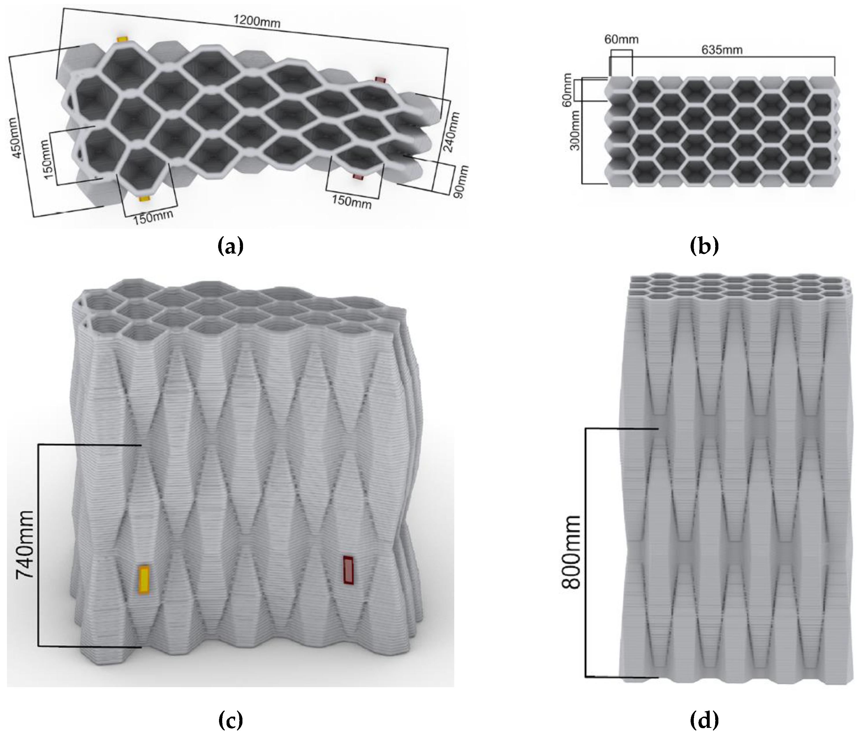
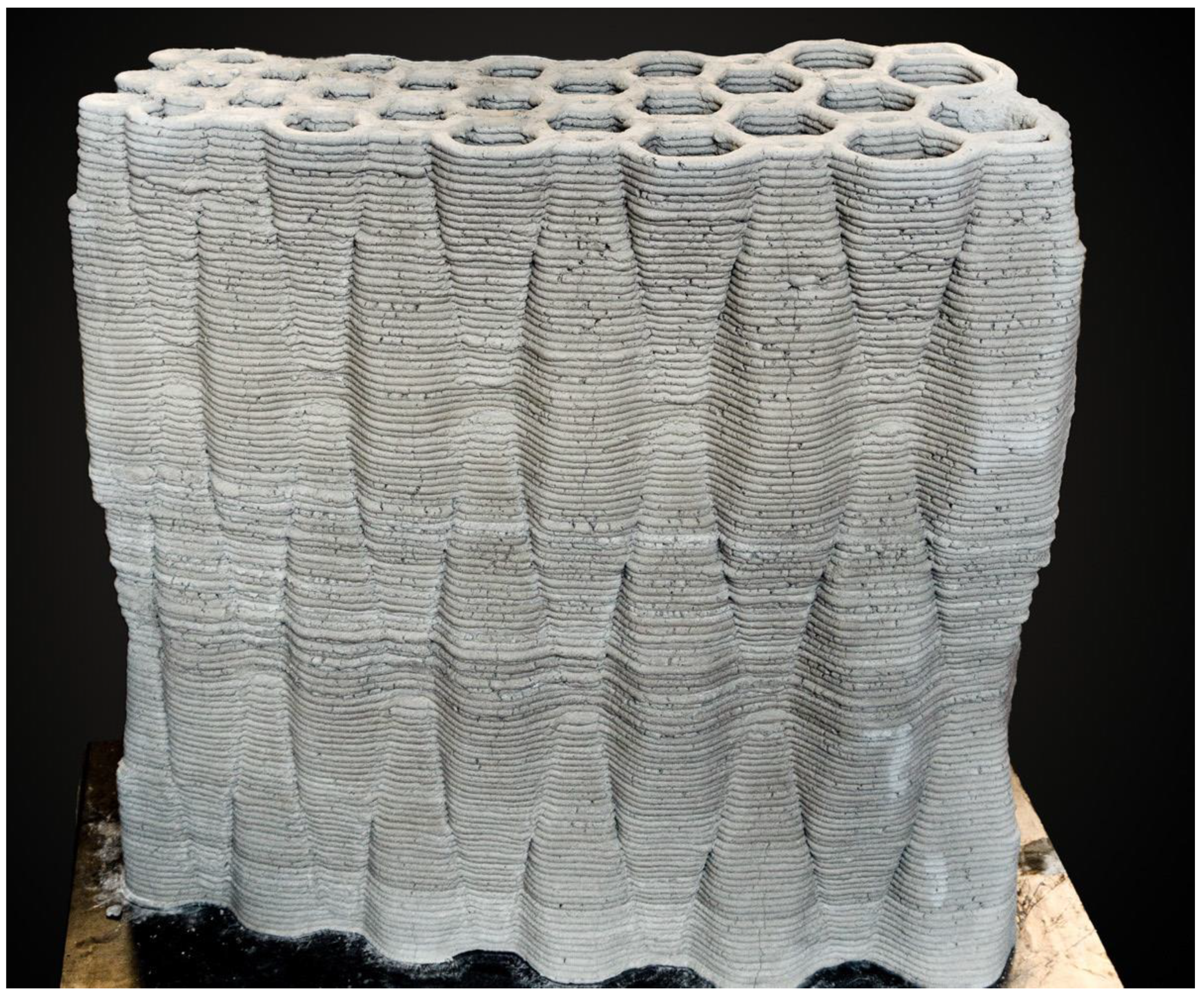
A tetrakaidecahedron, also known as a Kelvin cell [19], was chosen, aiming for a space filling topology with closed cells and a low ratio of surface area to volume (A/V ratio) for optimized thermal properties. The preceding studies resulted in the manufacturing of a prototype (see Figure 1), validating the design tool and printability [15]. This paper refers to that object as the existing prototype and uses it for further investigations, optimizations, and measurements.

2.3. Analytical Description of Heat Transfer in Cellular Solids

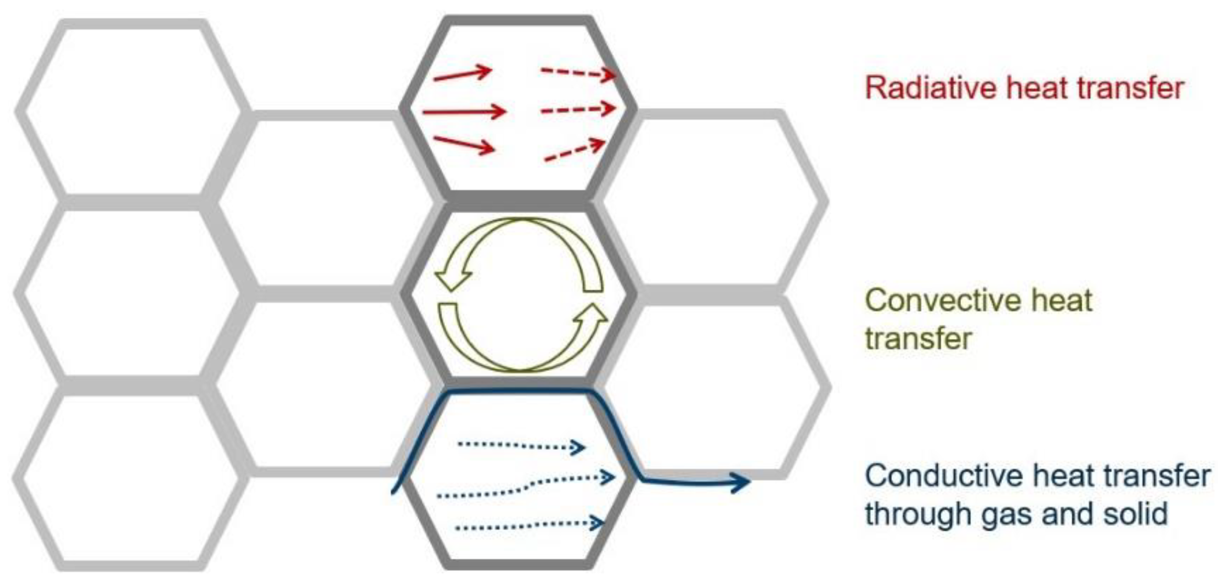
The evaluation of heat transfer through cellular solids [20], such as the cellular wall element, requires the determination of the following parameters, which are represented graphically in Figure 2:

• Solid conductivity (${\lambda }_{cond,solid}$);
• Gas conductivity (${\lambda }_{cond,gas}$);
• Radiation (${\lambda }_{rad}$);
• Natural convection (${\lambda }_{conv}$).

Figure 2. Heat transfer mechanisms in cellular structures, showing schematically radiative (red) and convective (green) heat transfer within the cells as well as conductive heat transfer (blue) through the gas (dotted line) and solid (continuous line).

Figure 2. Heat transfer mechanisms in cellular structures, showing schematically radiative (red) and convective (green) heat transfer within the cells as well as conductive heat transfer (blue) through the gas (dotted line) and solid (continuous line).

Relying on analytical expressions found in the existing literature, the total effective thermal conductivity ${\lambda }_{tot, eff}$ of a cellular solid consisting of all heat transfer mechanisms mentioned above is expressed in the form of its four constituents [21,22,23,24,25]:

$${\lambda }_{tot,eff}={\lambda }_{rad}+{\lambda }_{cond,gas}+{\lambda }_{cond,solid}+{\lambda }_{conv}$$

(1)

$$\begin{gathered} {\lambda }_{tot,eff}=\frac{16\ast \sigma \ast T^3}{3\ast 3.68\ast \frac{\sqrt{{\rho }_{rel}}}{b}}+F_p\ast \left[{\lambda }_{solid}\ast \left({\rho }_{rel}\right)+{\lambda }_{air}\ast \frac{0.18\ast G{r}^{\frac{1}{4}}}{{\left(\frac{h}{b}\right)}^{\frac{1}{9}}}\ast \left(1-{\rho }_{rel}\right)\right]+\left(1-F_p\right) \\ \ast \left[\frac{{\lambda }_{air}\ast \frac{0.18\ast G{r}^{\frac{1}{4}}}{{\left(\frac{h}{b}\right)}^{\frac{1}{9}}}\ast {\lambda }_{solid}}{{\lambda }_{air}\ast \frac{0.18\ast G{r}^{\frac{1}{4}}}{{\left(\frac{h}{b}\right)}^{\frac{1}{9}}}\ast \left({\rho }_{rel}\right)+{\lambda }_{solid}\ast \left(1-{\rho }_{rel}\right)}\right] \end{gathered}$$

(2)

with

$${\lambda }_{eff}={\lambda }_{cond,solid}+{\lambda }_{cond,gas}+{\lambda }_{conv}=F_p\ast {\lambda }_{parallel}+\left(1-F_p\right)\ast {\lambda }_{series}$$

(3)

$${\lambda }_{parallel}={\lambda }_{solid}\ast \left({\rho }_{rel}\right)+{\lambda }_{gas}\ast \left(1-{\rho }_{rel}\right)$$

(4)

$${\lambda }_{series}=\frac{{\lambda }_{gas}\ast {\lambda }_{solid}}{{\lambda }_{gas}\ast \left({\rho }_{rel}\right)+{\lambda }_{solid}\ast \left(1-{\rho }_{rel}\right)}$$

(5)

$${\lambda }_{gas}={\lambda }_{cond,gas}+{\lambda }_{conv}={\lambda }_{air}\ast Nu={\lambda }_{air}\ast \frac{0.18\ast G{r}^{\frac{1}{4}}}{{\left(\frac{h}{b}\right)}^{\frac{1}{9}}} (for \frac{h}{b}>3)$$

(6)

$${\lambda }_{rad}=\frac{16\ast \sigma \ast T^3}{3\ast K_{\lambda }}$$

(7)

$$K_{\lambda }=3.68\ast \frac{\sqrt{{\rho }_{rel}}}{b}$$

(8)

The optimization of specific geometric attributes reduces the total effective thermal conductivity inside a cell structure [26]. The thermal conduction through a cellular solid results from the combined conductivities of the gaseous and the solid phases of the structure, hence forming an average property for bulk material in the form of an apparent thermal conduction rather than a true material property [27]. The direction of heat flow within the cell arrangement influences the amount of apparent thermal conduction [22]. Hence, the geometric arrangement of the cells, expressed by the ratio of height to diameter and, therefore, the cell elongation, is an essential factor for the reduction of the thermal conductivity, in order to thermally optimize the structure aiming for a higher insulating effect, reduced heat losses, and thus more energy-efficient building operation.

The ratio of the density of a cell structure to the density of the solid forming the cell walls is defined as the relative density ${\rho }_{rel}$ [20]. By representing the solid share within the cell structure, this ratio ${\rho }_{rel}$ can be used to derive the respective share of the solid and gaseous phase of the total effective thermal conductivity of the cell structure. A reduction of the relative density decreases the mean thermal conductivity of the cellular solid considering the lower thermal conductivity of the gaseous material compared to the solid material.

Through the formation of closed cells with stagnant air, the influence of the convective heat transfer is reduced. The impact of free convection within the cells can be neglected entirely for geometries with a Grashof number (Gr) below 1000, i.e., with a low ratio of buoyant force to viscous force [28]. When solving the equation of the Grashof number for a minimum cell size, above which free convection becomes relevant, a critical value of 10 mm is obtained [28]. Since hollow Kelvin cells with a cell diameter of less than 10 mm cannot be manufactured by lightweight concrete extrusion due to overhangs and track width, the contribution of heat transfer induced by free convection inside the cell structure must be considered. In enclosed spaces, the amount of convective heat transfer across the cell can be quantified using the Nusselt number (Nu), defined as the ratio between the total effective conductivity of the fluid in motion and the thermal conductivity referring to a motionless fluid [23]. The formula of the Nusselt number, which includes the cell height h (z direction) as well as the cell size b (y direction), allows for the optimization of the cell size with regard to a minimized convective heat transfer. The analytical optimization, conducted through a linear approximation of the respective influence, results in a minimized thermal convection for vertically elongated cells. This is additionally supported by studies of the Nusselt number in dependence of the Rayleigh number for different aspect ratios h/b [29]. Further, the influence of the cell height on the total effective conductivity is found to be smaller than that of the cell diameter.

Measurements on polymer foams at room temperature show that 90% of the transmissivity is above the wavelength that is important for thermal radiation [25]. Hence, the radiative heat transfer component at room temperature is relatively small. It is therefore simplified in the analytical expression of the total effective thermal conductivity as follows: instead of the complex description of the radiative heat transfer equation in conjunction with the energy conservation equation [24], the commonly used Rosseland equation is applied, which describes an approximation of the radiative thermal conductivity. This approximation includes the Rosseland extinction coefficient of a cell structure, which is defined as the sum of the absorption coefficient and a weighted scattering coefficient of the foam. The extinction coefficient of a foam is calculated by forming the ratio of the square root of the relative density and the cell size, weighted by a given factor [25].

The parameters identified in this section that influence the thermal performance are, thus, the ratio of solid material to air, the diameter of the cells, the height of the cells, and the resulting cell elongation. A quantification of the respective influence and an optimization of the parameters will be conducted by means of a sensitivity analysis and a numerical optimization in Section 3.1 and Section 3.2.

2.4. Numerical 2D Heat Flux Analysis

Based on the theoretical background and analytical description in Section 2.3, where only a single resultant value ${\lambda }_{total, eff}$ can be calculated with a high geometrical simplification, a more detailed and locally resolved evaluation of thermal performance is enabled by two-dimensional heat transfer simulations. For this purpose, representative layers are selected and with the help of the Ladybug Tool Honeybee [30], XML files are created and used to simulate the heat flux within the heat-transfer analysis software LBNL THERM [31]. The algorithm behind THERM (Version 7.6) creates a mesh of discrete elements, defining the cross-sectional geometry, and performs a heat transfer simulation using a finite element solver. The equations used for the analysis are derived from the general energy equation, differentially considering the change in temperature over the change in location as well as internal heat generation inside the geometry [31]. The 2D simulation includes the heat transfer due to conduction and radiation via the finite element method (FEM) as well as a detailed view-factor-based radiation model [31]. By contrast, thermal convection is modeled by means of static, temperature-dependent surface heat transfer coefficients, based on natural convection correlations [32].

These calculations result in a locally boundary conforming mesh of temperatures and heat flux. In this way, THERM enables the calculation of a U-factor as a measure of the heat transfer through the cross section under defined environmental conditions. This is done by integrating the heat flux for a defined boundary segment or a group of segments and dividing that flux by the length of the segments as well as the defined temperature difference [32].

The boundary conditions include the temperatures on both sides of the studied object, as well as convection and radiation components on all surfaces (outer surfaces of the element or within the element itself). To allow a comparability of the results for the study, customized surface coefficients and boundary conditions regarding the exterior and interior surface of the studied objects were set to either fulfil the requirements defined in ISO 6946:2017-06 or to compare the simulated results with the measured ones by using the measured boundary conditions and surface coefficients.

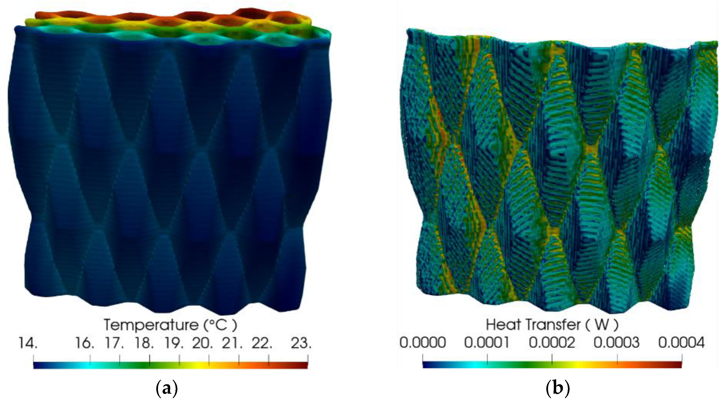
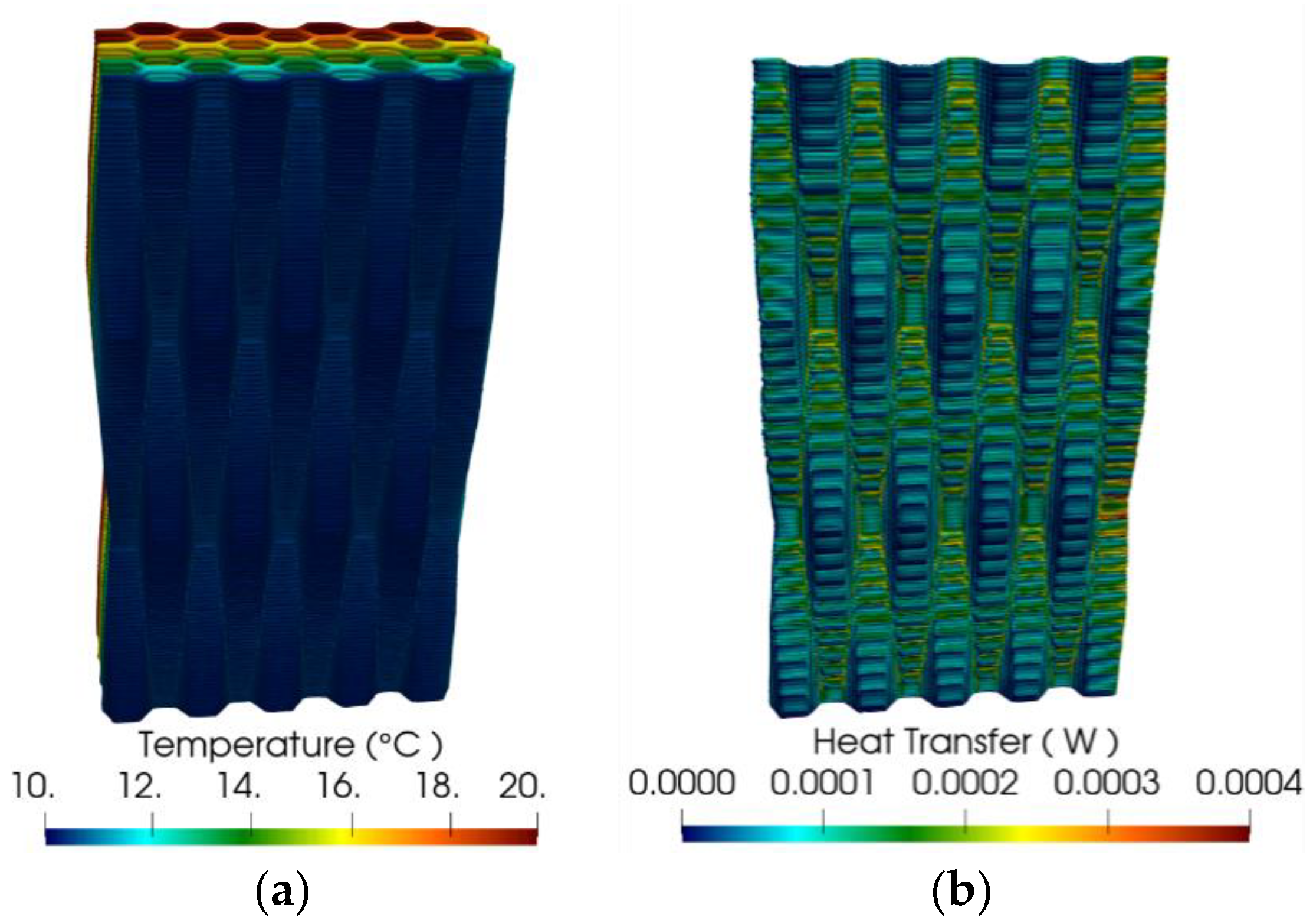
2.5. Numerical 3D Heat Flux Analysis

A supplementary procedure to the 2D numerical analysis with representative layers introduced in Section 2.4 is a 3D simulation where the whole geometry, as designed, constitutes the computational domain. While this approach requires significantly more computational power, it can provide additional insights that contribute to the validation of the experimental results, as discussed in Section 3.6.

Mesh generation for topologically complex structures in 3D is a challenging task for classical finite elements, especially if as-built geometries need to be accurately represented. An alternative method to the classical finite element method is the finite cell method (FCM) [33]. It allows for direct computational analysis on boundary representation (B-Rep) models such that the flaws and the imprecision in geometry can be correctly handled [34]. The finite cell method is an extension of the finite element method and embeds the physical domain ${\mathsf{\Omega }}_{phys}$ representing the artifact to be analyzed into a fictitious domain ${\mathsf{\Omega }}_{fict}$. Their union can then easily be meshed disregarding the boundary of the physical domain. 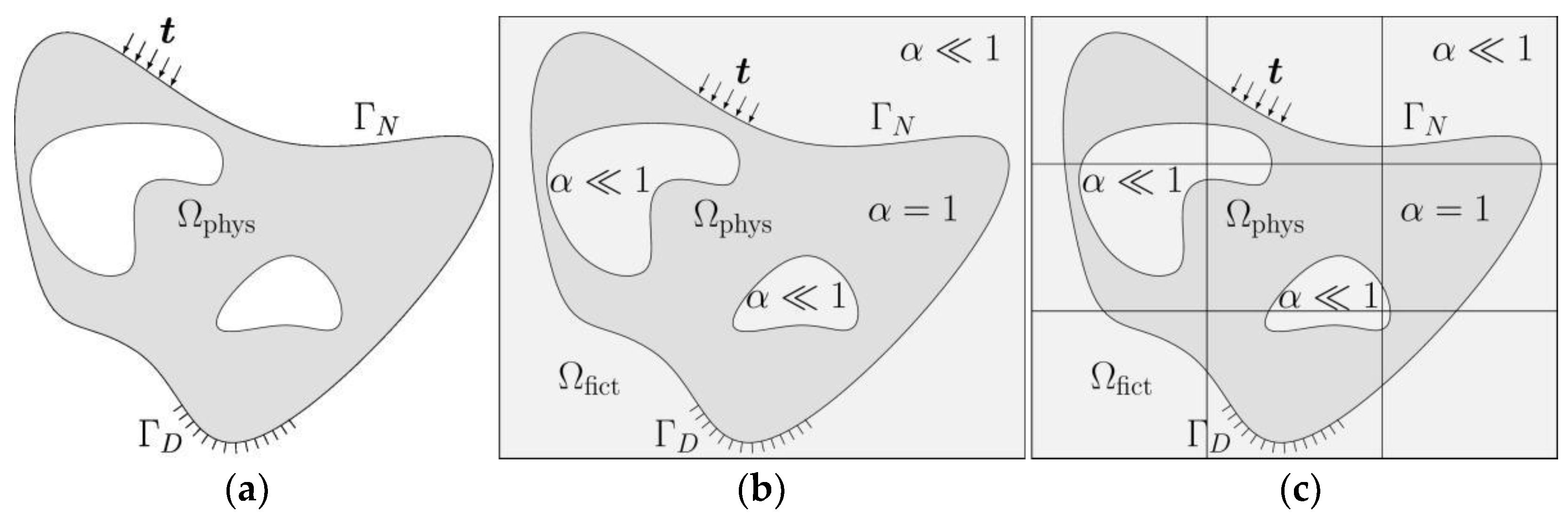The original geometry of the physical domain is resolved through an indicator function $\alpha \left(x\right)$, which relates a given position x with the physical or fictitious domain. The accurate resolution of the physical domain is then handled during the numerical integration, a process which is much easier to automatize than the boundary conforming mesh generation required by the finite element method. The FCM workflow is summarized in Figure 3, where a boundary value problem is defined on ${\mathsf{\Omega }}_{phys}$ with tractions t acting on the Neumann boundary ${\mathsf{\Gamma }}_N$ and the Dirichlet boundary condition is defined on ${\mathsf{\Gamma }}_D$ such that ${\mathsf{\Gamma }}_N\cap {\mathsf{\Gamma }}_D=\varnothing$ holds. The accuracy of FCM has been extensively studied in a variety of practical problems and was mathematically proven to be equal to the accuracy of the finite element method [35].

Within the scope of this contribution, the 3D FCM simulation (see Computer Code S1) computes the heat transfer due to conduction based on the steady-state heat equation, whereas the radiation and convection of air are modeled by static surface coefficients [14]. More specifically, an effective thermal conductivity coefficient ${\lambda }_{air,eff}$ is assigned to the air domain to model the convective and radiative heat transfer mechanisms.

The adoption of the air model with ${\lambda }_{air,eff}$ introduces a modeling error. An interval of U-values can be determined by taking the minimum and maximum plausible ${\lambda }_{air,eff}$ values and performing a series of simulations to capture the introduced errors. Defining such an interval is a practical approach to quantify the range of the modeling error introduced by the chosen air model. Thus, the U-values are reported with an associated interval for the sake of completeness.

The basic assumptions and simplifications adopted in 3D analysis closely follow the approaches employed in 2D analysis (see Section 2.4). The consistency between the two numerical approaches is further ensured with the definition of boundary conditions. The 3D simulation imposes the boundary conditions as laid out in Section 2.4 on the corresponding surfaces. This is analogous to the imposed boundary conditions on the lines in 2D simulation. Hence, requirements defined in ISO 6946:2017-06 are likewise fulfilled.

Similar to the 2D analysis, the main objective of the numerical study in 3D is to estimate the U-value of the whole wall element. To this end, the total heat flux on a specified surface area is calculated by integrating the local heat flux contributions and dividing by the area of the surface to find the heat flux density on the surface. The U-value is then calculated using the temperature difference and the heat flux density, as specified in ISO 15099:2003. The flexibility to choose a designated surface for the calculation of the U-value is especially convenient as the surface can be selected to match areas of interest, for instance where the heat flux is measured in the experimental setting (see Section 2.7). This allows for a local U-value calculation on a selected surface and results in a very accurate representation of the physical situation within the numerical analysis.

2.6. Experimental Thermal Conductivity Assessment

The thermal conductivity of the used lightweight concrete material is required as an input parameter for the solid conductivity ${\lambda }_{cond,solid}$ in the analytical approach (see Section 2.3) and as an initial value for the simulations. In parallel to the production of the element described in Section 2.1 and Section 2.2, lightweight concrete prisms were prepared. The thermal conductivity was determined using a dynamic measuring method. The hot disc method is specified in ISO 22007-2:2015-12 and is applicable for materials which have a thermal conductivity between 0.01 and 500 W/mK. The standard focuses on polymers, but the method can also be applied to other types of material.

In order to determine the thermal conductivity of the lightweight concrete, the Kapton sensor of the Hot Disk TPS 1500 was placed between two plane-parallel sawn halves of the specimen and heat was applied with 50 mW over 80 s. 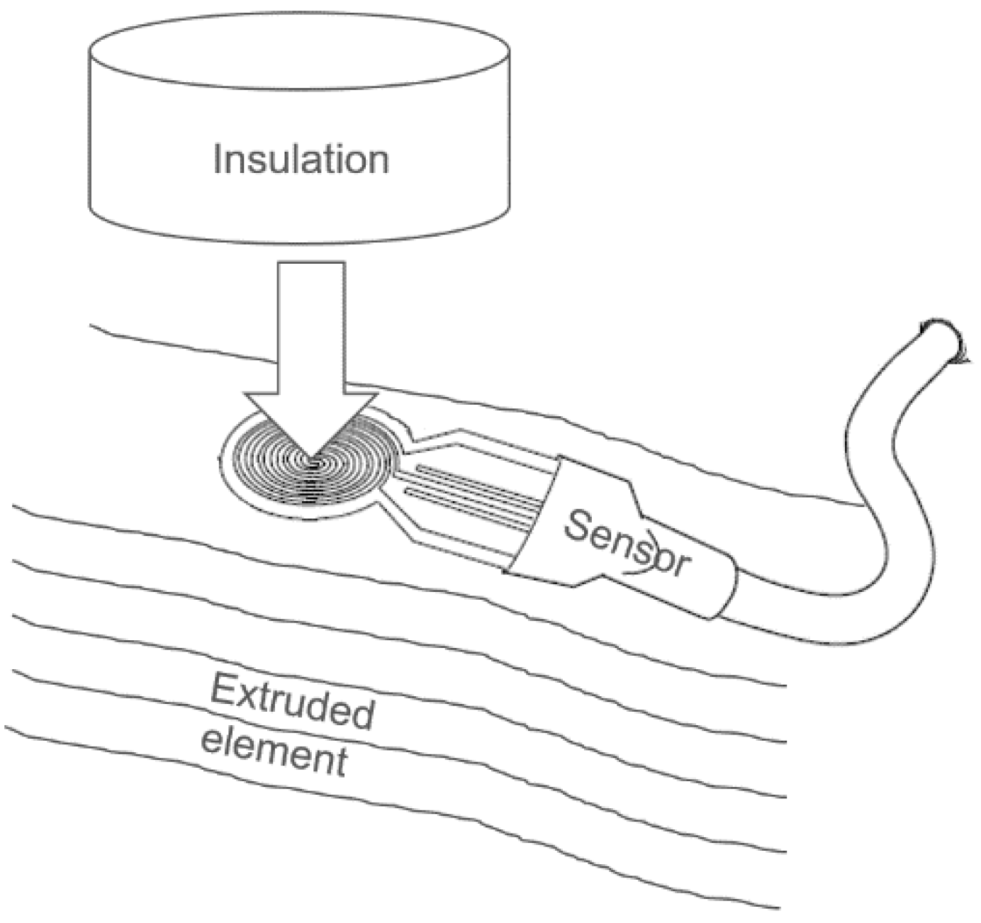The thermal conductivity can be calculated via the recorded heat dissipation $\lambda =P_{0 }/\left({\pi }^{3/2}\ast r\ast \mathsf{\Delta }{T}_s\left(\tau \right)\right)\ast D\left(\tau \right)$, where $P_0$ is the initial power, $r$ is the radius of the sensor, $D\left(\tau \right)$ is the dimensionless specific time function, and $\mathsf{\Delta }{T}_s\left(\tau \right)$ is the temperature increase on the specimen surface (see ISO 22007-2:2015-12). Since drying processes lead to deviations in the thermal conductivity of the material over time (0.44 W/mK after 14 days vs. 0.40 W/mK after 6 months), the thermal conductivity was additionally determined on the printed element itself at a comparable material age as the heat flux measurements (see Section 2.7) in order to be able to compare the numerical results with the experimental results. The same device (Hot Disk TPS 1500) was used for this measurement. As the sensor can only be placed on one side of the printed element, a highly heat-insulating material was applied and fixed on the opposite side of the sensor and a one-sided analysis was performed (Figure 4).

To compensate for the influence of an air gap or uneven surface, the material of the additively manufactured element was ground flat on an area slightly larger than the sensor. The measurements were conducted at an ambient temperature of 19 ± 2 °C. Thermal conductivity was measured three times each: perpendicular to the layers on the right side and on the left side of the element and parallel to the layers at the top of the last 3D-printed layer. The mean value was calculated in each case. As the hot disc method is an absolute measuring technology, no calibration of the system was necessary.

2.7. Experimental Heat Flux Measurements

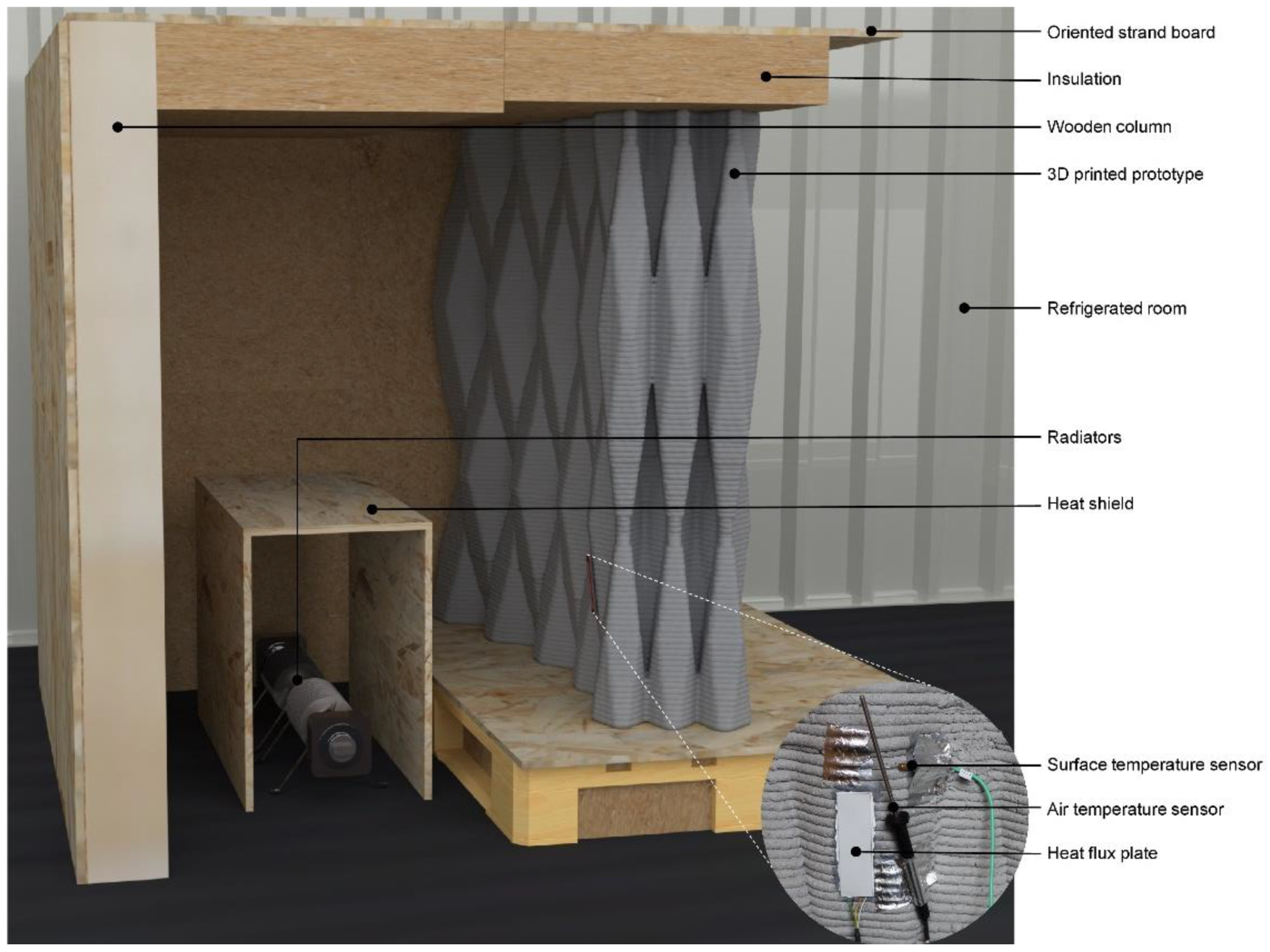
To validate the analytical and numerical approaches (as designed) and investigate the actual thermal performance (as built), the thermal transmittance of the element (U-value) was measured, which is defined in the ISO 7345 as the “Heat flow rate in the steady state divided by area and by the temperature difference between the surroundings on each side of a system”. The approach mainly follows the “Heat flow meter method” described in ISO 9869-1:2014, assuming a good estimate of the steady-state by averaging in situ measurements using a heat flow meter over a sufficiently long period. Since the tested object was transportable and not an immovable building component, the experimental setup was complemented with ideas of the “Calibrated and guarded hot box” in ISO 8990:1994.

The core requirements for the measurements and their implementation are summarized in

Table 1. Methodical requirements for the heat flux measurements [36] and their implementation in the conducted experiments.

Requirements	Implementation
Temperature difference between inside and outside $∆T\ge 10$ K	Temperature inside and outside controlled to remain at a constant level: $T_{ai}$ − $T_{ae}$ = 25 °C − 15 °C = 10 °C = $∆T$
Sufficiently long time interval of measurements (minimum 2 days)	Measurements are conducted over a time period of at least 48 h
Constant indoor temperature (about 20 °C)	The indoor temperature is controlled to remain between 23 °C and 25 °C
Small fluctuation of day/night temperature	The impact of external influences and day/night fluctuations is reduced by the surrounding refrigerated container
Reduction of external influences such as solar irradiation and humidity

. In order to achieve controlled boundary conditions, the test setup was located inside a refrigerated 20’ shipping container to provide stable boundary conditions over the course of the measurement. In order to create a temperature differential as a driver for the heat flux through the tested element, an insulated and heated enclosure was constructed, consisting of four sides around the prototype (12.5 mm oriented strand boards, construction lumber, and 120 mm wood fiber boards with $\lambda =0.38 \mathrm{W}/\mathrm{m}\mathrm{K}$). The construction is visualized in Figure 5.

The boundary conditions were controlled to remain in a set temperature range to achieve nearly steady-state conditions. The outside air temperature ($T_{ae}$) is defined as the air temperature of the refrigerated container, which was kept at 13 °C to 16 °C. The inner enclosure was equipped with two radiators (2 × 250 W) that were attached to a proportional-integral-derivative (PID) controller to regulate the indoor air temperature ($T_{ai}$) within 23 °C to 25 °C. An additional housing (12.5 mm oriented strand boards), which was left open on two sides, was built around the radiators to guarantee an even distribution of the heat and to avoid direct radiation to the measurement set up (see heat shield in Figure 5).

For the measurement setup itself, a calibrated digital heat flow plate (Ahlborn FQAD117T; calibration accuracy of 5% at nominal temperature of 23 °C) measured the heat flow density $q \left[\mathrm{W}/{\mathrm{m}}^2\right]$, with an integrated NTC (Negative Temperature Coefficient Thermistor) temperature sensor (±0.5 K at 0 °C to +80 °C) for automatic correction of the temperature coefficient. The heat flow plate was mounted on the inner surface of the wall element using a heat-conducting paste with a thermal conductivity of $10 \mathrm{W}/\mathrm{m}\mathrm{K}$ to compensate for the unevenness of the surface between the extruded filaments.

Air temperature and surface temperature were measured inside ($T_{ai}, T_{si}$) next to the heat flow plate and at the corresponding location on the outer wall surface ($T_{ae}, T_{se}$) using ice-bath calibrated temperature sensors (Ahlborn PT 100; 4-wire; ZA 9030-FS1; accuracy within ±0.05 K or 0.05% of measured value at −200 °C to +850 °C). Additional thermal cameras monitored the measurement qualitatively from the inside and outside.

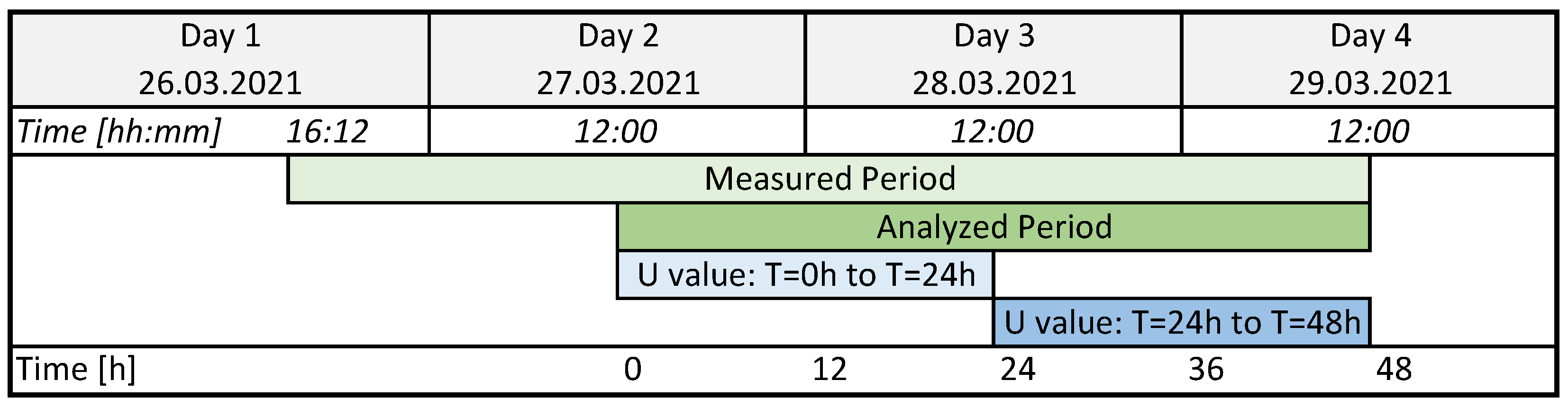
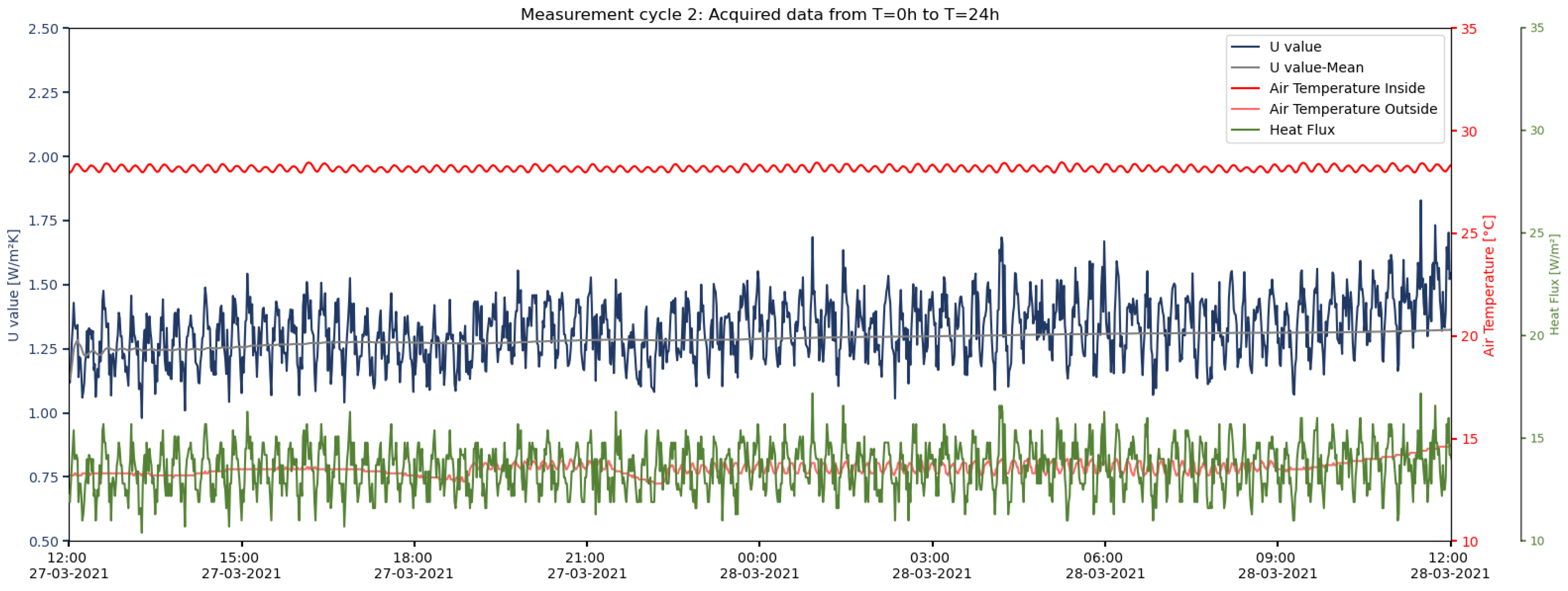
Following the average method (ISO 9869-1:2014), the acquired data over the total measured period were analyzed over time periods with integer multiples of 24 h (see Figure 6). All data sets were tested with respect to the conditions regarding the thermal resistance (R-value; see Equations (10) and (11)) defined in the standard to determine the applicability of the results for further evaluations:

• The R-value obtained at the end of the test does not deviate by more than ±5% from the value obtained 24 h before;
• The R-value obtained by analyzing the data from the first time period does not deviate by more than ±5% from the values obtained from the data of the last time period of the same duration.

Figure 6. Schematic timeline for the data evaluation of the heat flux measurements (measurement cycle 2) according to the average method (ISO 9869-1:2014); showing the measured period (light green), the analyzed period (dark green), and the respective subdivided time periods (blue).

Figure 6. Schematic timeline for the data evaluation of the heat flux measurements (measurement cycle 2) according to the average method (ISO 9869-1:2014); showing the measured period (light green), the analyzed period (dark green), and the respective subdivided time periods (blue).

Generally speaking, the thermal transmittance (U-value) of a building component describes the amount of heat flowing through a surface area of 1 m² within one second, with a deviation of steady-state air temperatures on both sides of 1 K [36]. The corresponding total thermal resistance R sums up all thermal resistances of individual material layers and the thermal resistances on both surfaces of the component (see Equation (9)). Since this theoretical assumption is only valid for equilibrium state, its application for the experimental evaluation is limited [36]. As a result, the U-value calculation was based on a cyclic acquisition of the mean temperature values and the mean values of the heat flux density (see Equation (11)) [36,37]:

$$U=\frac{1}{R_t}=\frac{1}{R_i+R+R_e}=\frac{1}{\frac{1}{{\alpha }_i}+\frac{1}{\mathsf{\Lambda }}+\frac{1}{{\alpha }_e} } \left[\frac{W}{m^{2}K}\right]$$

(9)

$$R=\frac{T_{si}-T_{se}}{q} \left[\frac{m^{2}K}{W}\right]$$

(10)

$$\overline{R}=\frac{{\sum }_{j=1}^n\left(T_{sij}-T_{sej}\right)}{{\sum }_{j=1}^n{q}_j} \left[\frac{m^{2}K}{W}\right]$$

(11)

$${\alpha }_i=\frac{q}{T_{si}-T_{ai}} \left[\frac{W}{m^{2}K}\right]$$

(12)

$${\alpha }_e=\frac{q}{T_{se}-T_{ae}} \left[\frac{W}{m^{2}K}\right]$$

(13)

$$\mathsf{\Lambda }=\frac{q}{T_{si}-T_{se}} \left[\frac{W}{m^{2}K}\right]$$

(14)

3. Results

3.1. Sensitivity Analysis

To quantify the degree to which the individual geometric parameters affect the total effective thermal conductivity of a cellular solid, a global sensitivity analysis according to the method of Sobol’ [38] was conducted. The analytical description of the total effective thermal conductivity (see Section 2.3) is defined as the input function $y=f\left(x\right)=f\left(x_1, x_2, \dots , x_k\right)$ with the model output $y$ as the total effective thermal conductivity, the function $f$ as the analytical description, and a vector of $k$ input factors $x=\left(x_1, x_2, \dots , x_k\right)$ as the geometric parameters. The studied parameters are as follows:

• Extinction coefficient of the cellular solid;
• Relative density;
• Cell wall thickness;
• Cell diameter;
• Cell size.

Plausible ranges were defined for the individual parameters. Using the open-source Python library SALib (v1.3.12) [39] the fractions of the total variance of the function $f\left(x\right)$ were deduced in the form of sensitivity indices of the first ($S_1$) and second order. Total-order indices ($ST$) describe the interaction between the parameters while confidence intervals ($S_{1,conf}$, $S{T}_{conf}$) quantify the uncertainty of the estimates of the indices (see

Table 2. Resulting sensitivity indices of the conducted analysis for the parameters influencing the total effective thermal conductivity.

Notation	Parameter	${\mathit{S}}_1$	${\mathit{S}}_{1,\mathit{c}\mathit{o}\mathit{n}\mathit{f}}$	$\mathit{S}\mathit{T}$	$\mathit{S}{\mathit{T}}_{\mathit{c}\mathit{o}\mathit{n}\mathit{f}}$
x1	Extinction coefficient	0.000	0.000	0.000	0.000
x2	Relative density	0.459	0.012	0.518	0.012
x3	Cell height	0.003	0.001	0.004	0.001
x4	Cell diameter	0.479	0.135	0.537	0.011

).

The results indicate that the highest influence on the total effective thermal conductivity stems from a change in the relative density and the cell diameter, with more than 90% of the output variance attributed to their variance. The confidence intervals of the sensitivity indices—giving insights on the validity of the results—differ between the parameters: while the confidence intervals of the first and total order indices of the cell height, the relative density, and the extinction coefficient were below a threshold of 10% (indicating a good reliability of the results), the confidence interval of the first order indices of the cell diameter was at 13.5%, suggesting a relatively high inaccuracy of the result. A further focus will, therefore, be put on optimization of the cell size, especially the diameter, as well as the relative density.

3.2. Parametric Optimization

By adjusting the identified parameters, the thermal performance of the cell structure was optimized. For this purpose, the objective, the variables, and the existing constraints were identified, a process known as modeling [40]. The findings of the sensitivity analysis (see Section 3.1) were applied in an optimization focused on the adjustment of the relative density as well as the cell size in the form of the diameter and the height. The parameter indices, units, and constraints are defined in

Table 3. Parameter allocation for the parametric optimization of the cellular solid.

Index	Parameter	Unit	Constraints
x0	Relative density	(-)	$\{x0\in ℝ :0.2\le x0\le$0.8}
x1	Cell height (z)	(mm)	$\{x1\in ℝ :300\le x1\le$ 800}
x2	Cell diameter (x and y)	(mm)	$\{x2\in ℝ :50\le x2 \le$ 800}

.

Given the nature of the present model describing the heat transfer coefficient through a cellular solid (see Section 2.3) and its specific boundary conditions—arising from the AM process and from material properties—that constrain the input range of the variables, a constrained model and the corresponding optimization algorithm were chosen. The optimization was computed using the Python library “Scipy.Optimize”. By means of a trust-region algorithm that enables versatile usages and is especially appropriate for large-scale problems [40], the total effective conductivity was minimized with regard to the chosen parameters. To diminish the influence of uncertainties, the search area was restricted to a region, where the approximation was assumed to be located. Additionally, and in an effort to help the optimizer to avoid local optimization-minima, different starting points were used.

The optimization resulted in an exact definition of the relative density: independent of the starting point, a minimized heat transmission occurred in structures with a relative density of 0.2, validating the assumption made in Section 2.3 that a low relative density reduces the total effective conductivity.

The optimization, however, did not yield a clear result for the quantified optimum of the cell diameter. Depending on the starting point of the optimization (x_start) and the cell height, different configurations for an optimized diameter were computed. Overall, the results can be summarized to be located in the range between 50 mm and 120 mm with a tendency towards smaller cell diameters. This inaccuracy of the results can be explained by the relatively high confidence interval that was computed in the sensitivity analysis (see Section 3.1 and Table 2). Since the cell diameter is an essential factor that helps minimize the heat transfer, computational parametric 2D thermal simulations (compare Section 2.4 and Section 3.4) were additionally conducted, resulting in a thermally optimized cell diameter of 70 mm. A further reduction of the cell diameter did not yield a further reduction of the total effective conductivity.

To ensure a good comparability of the thermal performance of the optimized structure with that of the existing prototype, efforts were made to achieve the same overall wall thickness of the element. Due to the curved outline and the varying total thickness of the existing prototype, a comparable average value was set to 300 mm. An overall wall thickness of 300 mm can be reached for an optimized prototype with a cell diameter of 60 mm and a cell count of four cells. The resulting geometric characteristics for the chosen parametric optimization of the cellular solid are shown in

Table 4. Geometric characteristics of the manufactured demonstrator and for a thermally optimized cell configuration.

Geometric Characteristic	Demonstrator	Optimization
Base dimensions in (mm)	1200 × 800	-
Element height in (mm)	1040	-
Layer count (-)	116	-
Layer height in (mm)	9	-
Cell height in (mm)	740	800
Cell diameter in (mm)	90–150	60
Cell wall thickness in (mm)	19	12
Resulting relative density (-)	0.31	0.48
Cell count (-)	2/3	3/4 or higher
Total wall thickness in (mm)	240–450	300

and Figure 7 and contrasted with the manufactured demonstrator.

Similarly to the investigation of the cell diameter, the cell height h was tested for different starting points to ascertain any inaccuracies and dependencies. The results obtained from the numerical optimization yielded an exact value for the optimized cell height of 800 mm. This resulted in a vertical elongation of the cells, which is also predicted to be favorable in the theoretical study of the heat transfer through the comparison of different cell wall arrangements. This assessment resulted in a favorable ratio of cell height h to cell size b of h/b > 2. Additionally, a decrease in the relative density was achieved through a high value of the cell height, as the ratio of solid material to air in the structure was decreased.

3.3. Results of Thermal Conductivity Assessment

The thermal conductivity measured on the right side of the additively manufactured element was on average 0.38 W/mK and on the left side on average 0.39 W/mK with a standard deviation of 0.03 W/mK on each side. Measured parallel to the layers from the top, a mean thermal conductivity of 0.37 W/mK was determined with a standard deviation of 0.02 W/mK. Thus, within the limits of measurement accuracy, there were no differences in thermal conductivity across the additively manufactured element. The overall mean of 0.38 W/mK served as a basis for further investigations and as an input parameter for all analytical and numerical approaches.

3.4. Results of Heat Flux Measurements

Over the course of this, study three measurement cycles were conducted, with two analyzed periods of 24 h each and a total measured period of 55 h, 64 h, and 70 h, respectively. These time series are exemplarily shown in Figure 6. Cycles 1 and 3 were carried out at the same location at the wider side of the element but with an optimized test setup in cycle 3, improving the insulation of the baseplate to reduce the disruptive effects of a thermal bridge after the initial findings of the first cycle. For the second measurement, the sensors were positioned at the slimmer side of the demonstrator at the same height in order to take account of the varying thermal performance due to the geometrical variation (see Figure 7). The varying cell sizes in the printed specimen as well as the curved and widening geometry require special attention, as the location of the assessment has significant impact on the resulting U-value.

The deviations of $R\left(t=48 \mathrm{h}\right)$ to $R\left(t=24 \mathrm{h}\right)$ as well as $\overline{R}\left(2\mathrm{n}\mathrm{d} 24 \mathrm{h}\right)$ to $\overline{R}\left(1\mathrm{s}\mathrm{t} 24 \mathrm{h}\right)$ for the first and third measurement cycle were found to be above the 5% threshold defined in the ISO standard (see Section 2.7). Suspected and/or detected errors, inducing theses deviations, are lacking and inconsistent measurement values due to malfunctions of the sensor equipment (cycle 3), fluctuations in the external temperature due to the regulation of the container’s air-conditioning (cycle 3), and thermal bridge effects at the base plate (cycle 1) causing an aberrant thermal heat flux close to the measurement device, which was optimized after the first cycle. The second measurement cycle showed the most promising results, even though the deviation of the R-value exceeded the threshold slightly with 9%. The mean values, however, fulfilled this condition with a deviation of 4% and thus an evaluation according to the average method described in the ISO 9869-1:2014 and Section 2.7 seems reasonable.

The results for the second measurement are visualized in Figure 8 and Figure 9, showing the measured heat flux, air temperature inside and outside, and the derived U value, split into the two analyzed time periods. Despite a marginal rise in the outside air temperature in the beginning of the second half of the analyzed period, the overall boundary conditions were found to be very stable. The relevant collected data and resulting thermal properties are compiled in

Table 5. Collected data and resulting thermal properties for single time steps.

Time [h]	${\mathit{T}}_{\mathit{s}\mathit{i}}$ (°C)	${\mathit{T}}_{\mathit{a}\mathit{i}}$ (°C)	${\mathit{T}}_{\mathit{s}\mathit{e}}$ (°C)	${\mathit{T}}_{\mathit{a}\mathit{e}}$ (°C)	$\mathit{q}$ (W/m2)	$\mathit{U}$ (W/m2 K)	$\Lambda$ (W/mK)	$\mathit{R}$ (m2 K/W)
0	25.9	28.0	14.4	13.2	12.2	1.15	1.06	0.94
24	26.1	28.3	15.4	14.7	14.2	1.55	1.33	0.75
48	26.3	28.4	15.9	15.3	15.4	1.73	1.48	0.68

for single time steps (0, 24 h, 48 h) as well as the mean values for the total analyzed period and its two moieties separately in

Table 6. Mean values of the thermal properties derived from the collected data over the analyzed time periods.

Period $(-)$	${\mathit{T}}_{\mathit{s}\mathit{i}}$ (°C)	${\mathit{T}}_{\mathit{s}\mathit{e}}$ (°C)	$\mathit{q}$ (W/m2)	$\overline{\mathit{U}}$ (W/m2 K)	$\overline{\mathit{R}}$ (m2 K/W)
0 to 24 h	26.0	14.8	13.6	1.32	0.83
24 to 48 h	26.2	15.7	13.3	1.41	0.80
Analyzed period	26.1	15.2	13.5	1.37	0.81

. In essence, the measured thermal performance, represented by the mean U-value for the overall analyzed period, accounted for 1.37 W/m² K.

Due to the curved and widening geometry of the wall, deviations of thermal performance at both measurement locations are anticipated, because of the varying cell size, total wall thickness, and relative density. In spite of the exceeded thresholds according to the standard, the mean U-value of the third cycle with 0.75 W/m² K is also used with reservation for a general overview and is compared to local U-value assessment using the 3D simulations (see Section 3.6).

3.5. Results of the 2D Simulations

By calculating the heat flux within a finite element mesh for individual layers of the element, two-dimensional heat flux simulations (see Section 2.4) allow a 2D visualization of the thermal performance. In Figure 10, results are shown for one respective layer of the existing prototype and the optimized geometry (see Section 3.2). The geometric discretization via the finite element mesh is challenging, especially for the highly complex and irregular geometry of the existing prototype (see Figure 10 top). The visualization of the heat flux clearly shows a concentration of heat transfer within the cell walls bridging across the element in the y-direction with values around 10–20 W/m² K (light blue to green). The heat flux within the cavities and the cell walls parallel to the element in x-direction was mostly below 10 W/m² K (purple to dark blue). Comparing the existing prototype to the optimized geometry, the increase of cell count and the decrease of cell diameter are reflected in the visual results, showing lower heat flux (less blue) within the cavities. Due to the varying total wall thickness of the existing prototype, the heat flux across the element through the cell walls was higher on the narrower left part (more green) but lower at the wider right part (less light blue) compared to the more uniform optimized geometry. On the edges of both geometries, higher heat flux values were visualized, especially for the existing prototype at the two sharp concave edges. This is presumably due to the chosen adiabatic boundary conditions at these element joints, leading to a concentration of heat flux in the adjacent strands, since no heat transfer is happening with the adiabatic boundary and thus the possible heat flow directions are limited.

3.6. Results of the 3D Simulations

The 3D heat flux simulation (see Section 2.5) enables the computation of U-values as a measure for the heat transmittance through the element evaluated for specific surface areas, offering additional flexibility. Following the conducted heat flux measurements, the following surface areas can be chosen for a U-value calculation:

• The total surface area of the wall element;
• The surface area of the heat flux plate for measurement cycle one and three;
• The surface area of the heat flux plate for measurement cycle two.

To get an average view of the thermal performance of the entire wall element, the U-value can be evaluated for the total wall surface area. In addition, taking into account the local surface areas of the heat flux measurements allows for the accounting of varying thermal performance due to geometric deviations in cell size, total wall thickness, and thus relative density, both horizontally and vertically. In other words, the physical experiments use a measurement device that quantifies the local heat flux close to its surface; thus, the derived U-value characterizes the local thermal transmittance through the respective location. Analogously, a surface area corresponding to the measurement device can be chosen in the computational domain to estimate the local heat flux and to calculate a local U-value, facilitating a one-to-one comparison between the computational results and the measurements (see Section 3.7).

The U-value on the entire wall surface of the existing prototype was computed as 0.77 W/m² K and the corresponding computational results are depicted in Figure 11. An associated interval (see Section 2.5) was found to be [0.67–0.89].

The local U-values evaluated on the surface according to the second and third measurement cycle amounted to 1.10 W/m² K and 0.60 W/m² K with associated intervals of [0.99–1.22] and [0.55–0.68], respectively. The high U-value on the surface of the second assessment, depicted in Figure 7, can be explained by the geometry of the wall element, as it was conducted on a surface area where the cell diameter and total wall thickness were the smallest and the heat transfer took place more effectively. In contrast, the third assessment was conducted on a surface area where the cell diameter and total wall thickness were the largest (see Figure 7); therefore, the calculated U-value had a lower value, which also complies with the results of the 2D simulations (see Figure 10).

While the geometrically optimized design (see Section 3.2) was not yet manufactured, the thermal performance of the design was similarly analyzed to validate the improved thermal properties. The U-value of the optimized design was computed on the whole wall surface and it accounted for 0.61 W/m² K with an associated interval of [0.55–0.70]. The corresponding visual 3D simulation results are depicted in Figure 12.

3.7. Comparison and Verification

The results of the 2D and 3D simulations as well as the analytical assessment for the existing prototype and the optimized structure are compared and the local values are validated with the results from the heat flux measurements (see Figure 13). The varying cell sizes in the printed specimen as well as the curved and widening geometry require special attention, as the location of the assessment has a significant impact on the resulting U-value.

By considering a representative layer, the 2D analysis provides an average U-value for the whole wall element (Prototype Total and Optimized Total) that is independent of the sensor location. The variance of the layerwise analysis due to vertical discrepancies was found to be $\pm$7%. The 3D analysis evaluates the heat flux for the whole element and additionally allows taking into account the location of the sensor and assessing the U-value at the respective sensor surfaces (see Section 3.5). This can be compared to the measured values (Prototype Cycle 2 and Prototype Cycle 3), whereas the local assessment is not applicable for the 2D simulations, since the layerwise evaluation neglects local discrepancies in the vertical direction.

The results for the whole wall element (Prototype Total) show a very high correspondence between the 2D, 3D, and analytical approach with U-values in the range of 0.75–0.77 W/m² K ($\le$3% deviation). The geometrical optimization (Optimized Total) resulted in U-values of 0.58–0.64 W/m² K ($\le$10% deviation), also showing a good match of all three approaches. Thus, the optimization resulted in improvements of 15–24% compared to the existing prototype with a comparable total wall thickness (see Table 4 and Figure 7).

The locally evaluated results of the 3D analysis clearly suggest that the wider part of the element had a better thermal performance by 45% (0.60 W/m² K for cycle 2) compared to the narrower part (1.10 W/m² K for cycle 3). This complies with the theory in Section 2.3 and findings in Section 3.4. Taking into account the computed U-value for the whole element (0.77 W/m² K), it can be observed that the overall performance lies between the two local results. Comparing the measured U-value of cycle 2 (1.37 W/m² K) to the respective locally evaluated value of the 3D analysis (1.10 W/m² K), a fairly high correspondence with a deviation of 25% can be detected. The same deviation can be found for the local values of cycle 3 (0.75 W/m² K—measured; 0.60 W/m² K—3D simulation), underlining the applicability of this approach despite the reservations for measurement cycle 3 regarding the exceeded thresholds (see Section 3.4).

4. Discussion

The idea and the potential of combining additive manufacturing with lightweight concrete and thereby creating extruded mono-material, multi-functional wall elements are underlined and supported by this study. Using the advantages of the automated AM process of lightweight concrete extrusion, the geometry of a wall element can be optimized, reducing the material use by creating a complex cellular solid with an optimized insulating functionality without the necessity of multiple layers and using only one material, enhancing recyclability. Since simple methods to evaluate the thermal performance of building elements—such as ISO 6946:2017—are not applicable to such complex geometries, this paper demonstrates several alternative, more detailed evaluation methods: an analytical approach, layerwise 2D simulations, 3D simulations, and heat flux measurements.

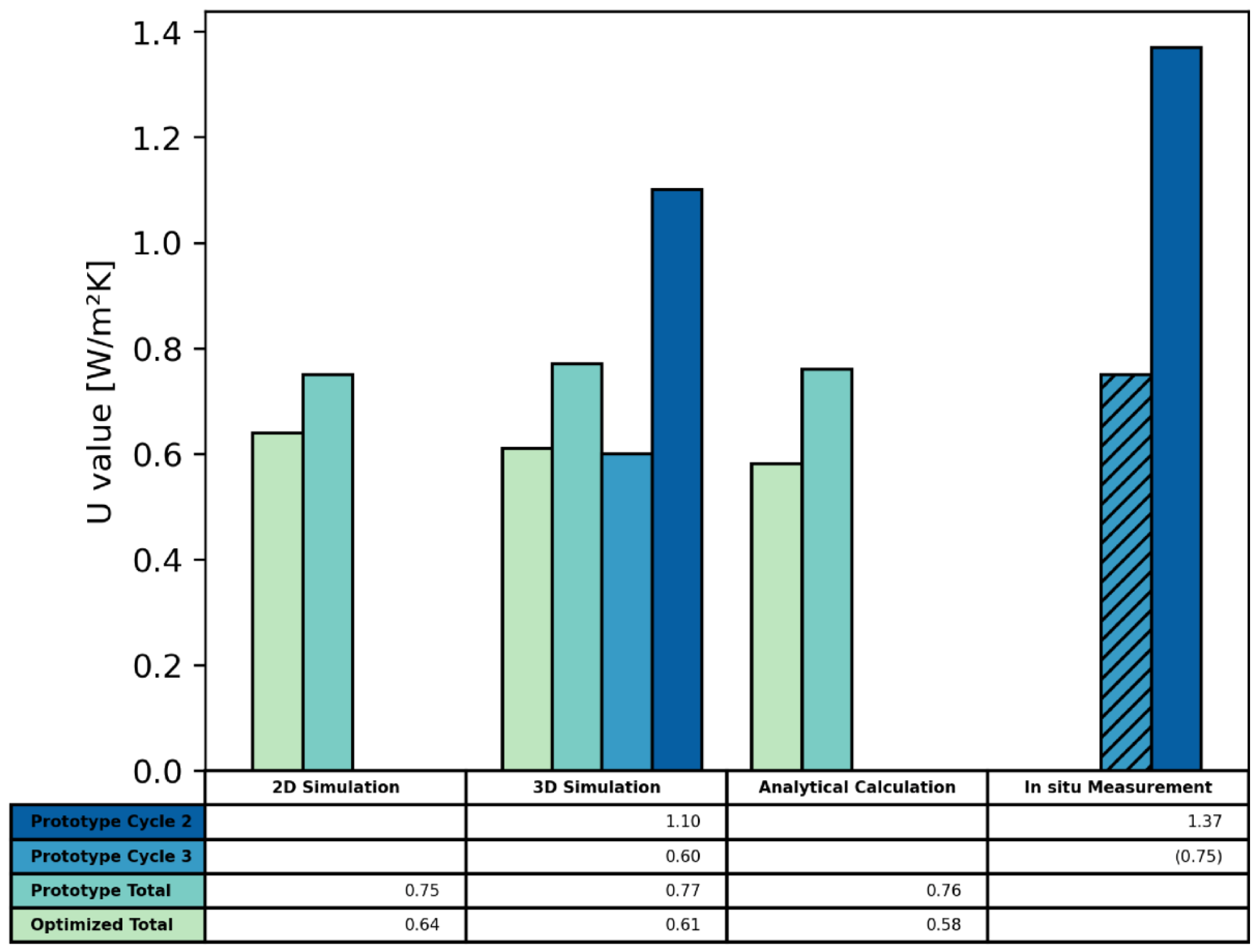
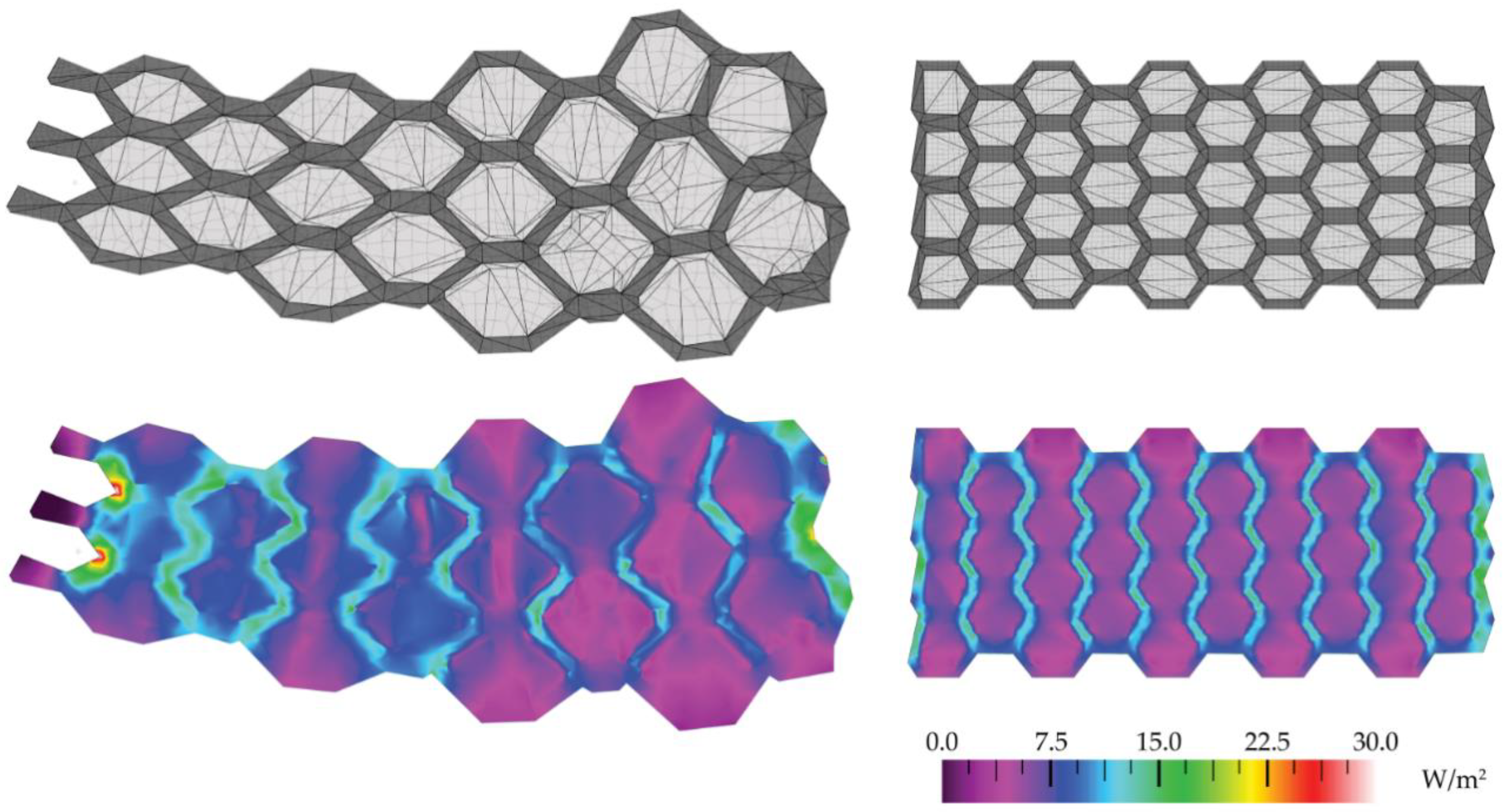
Using an existing AM prototype, these approaches were applied to evaluate its thermal properties and to further optimize its geometry. The comparison of the results showed a high correspondence of all three theoretical approaches among each other (2D and 3D simulation, analytical approach) with 3 to 10% deviation, indicating their appropriate application. Looking more closely into the methods themselves revealed individual strengths and limitations as well as specifically suitable use cases. The analytical approach, which can be seen as the most simplified one due to its geometrical simplification, is particularly suitable for mathematical optimization techniques due to its negligible calculation effort; however, it enables only a single resultant value. In contrast to this solely analytical description, the 2D simulation additionally allows for visualization of the heat flux within a finite element mesh and thus also enables local interpretation of thermal properties. This is essential for highly complex geometries, such as the one presented in this study. Furthermore, this method is directly embedded in the design workflow, facilitating a highly automated and fast feedback loop within the design process. On the downside, the limiting factors are that only one representative layer can be evaluated at once, the cell height is not taken into account, and the influence of convection within the air voids is not calculated explicitly. The approach of 3D computations adds the missing vertical dimension to the evaluation, allowing an overall view of the thermal performance of the whole wall element. At the same time, this enables a local assessment of designated areas of interest, for instance, in the sense of a “hot spot analysis” for moisture problems or complex three-dimensional thermal bridges in general [41,42]. Even though the convective heat transfer is not yet implemented and the thermal conductivity of air in the cells is simplified, the results already show a very promising validity.

The initial assumption, that the actual measured performance (as built) is lower than the theoretically assessed properties (as designed) due to inaccuracies of the extruded concrete strands (cracks and cavities), was verified. In general, the experimental U-value evaluation using heat flux measurements and its comparison to the simulated results showed the validity and applicability of the theoretical approaches. The deviation of 25% can be traced back to several potential error sources. Inaccuracies of the printed object, especially regarding the layer thickness, layer height, and the print paths themselves, lead to geometrical deviations between as built and as designed. Moreover, the cracks caused by the drying process of the lightweight concrete and imperfections in general due to irregularities during the extrusion process are assumed to influence the local thermal properties. Furthermore, the complex geometry and uneven surface of the printed object are challenging for the measurement process. In combination with demanding and sensitive boundary conditions as well as required long measurement periods, this leads to the limitation that only one out of three measurement cycles can be evaluated without or with little reservations. Further improvements of the measurement setup and a larger number of measurements over a longer period on several locations would be needed for an even more reliable validation of theoretical and experimental results. Additionally, further studies on the discrepancies between as designed and as built could be realized using laser scanner and point clouds.

In general, the cellular solid geometry of the existing prototype was further optimized using the approaches mentioned above. The optimization resulted in a reduction of the U-values by about 20%, accounting for approximately 0.6 W/m² K at a comparable total wall thickness of 30 cm. The printability of the optimized geometry will be subject to future research as well as the validation of its target performance by improved measurements.

5. Outlook

In combination with the possibility of grading the material properties (e.g., with respect to their thermal conductivity and load-bearing capacity), components could be designed completely freely and the locally required material properties could be determined via simulations in order to achieve a consistent U-value along the whole element. Similarly, complex connection situations (e.g., wall/floor or inner/outer wall) could be improved by using material grading and an optimized internal cellular solid structure. In general, the approach of optimizing the internal structure with regard to thermal performance can be combined with common topology optimization for its structural behavior.

Furthermore, the presented study can pave the way for bringing AM in construction to the next level by integrating additional active functions within AM wall elements. Active functions could be added by directly integrating ducting or channeling for heating, cooling, and/or ventilation purposes. For this objective, the presented approaches for performance evaluation by modeling and measurements as well as geometric optimization are essential.

References

1. Knaack, U. Building Physics of the Envelope: Principles of Construction; Walter de Gruyter GmbH: Basel, Switzerland; Berlin, Germany; Boston, MA, USA, 2018; ISBN 9783035609493. [Google Scholar]
2. Herzog, T.; Krippner, R.; Lang, W. Facade Construction Manual, 2nd ed.; DETAIL: München, Germany, 2018; ISBN 9783955533700. [Google Scholar]
3. Labonnote, N.; Rønnquist, A.; Manum, B.; Rüther, P. Additive construction: State-of-the-art, challenges and opportunities. Autom. Constr. 2016, 72, 347–366. [Google Scholar] [CrossRef]
4. Paolini, A.; Kollmannsberger, S.; Rank, E. Additive manufacturing in construction: A review on processes, applications, and digital planning methods. Addit. Manuf. 2019, 30, 1–13. [Google Scholar] [CrossRef]
5. Menges, A. Manufacturing Performance. Arch. Des. 2008, 78, 42–47. [Google Scholar] [CrossRef]
6. Holger Strauss. AM Envelope: The potential of Additive Manufacturing for facade constructions. Archit. Built Environ. 2013, 1, 1–270. Available online: https://journals.open.tudelft.nl/abe/article/view/strauss (accessed on 14 July 2022).
7. Piccioni, V.; Turrin, M.; Tenpierik, M.J. A Performance-Driven Approach for the Design of Cellular Geometries with Low Thermal Conductivity for Application in 3D-Printed Façade Components. In Proceedings of the Symposium on Simulation for Architecture and Urban Design (SimAUD 2020); Chronis, A., Wurzer, G., Lorenz, W.E., Herr, C.M., Pont, U., Cupkova, D., Wainer, G., Eds.; Society for Computer Simulation International (SCS): Vienna, Austria, 2020; pp. 327–334. Available online: http://resolver.tudelft.nl/uuid:07b77206-404d-41dc-b55e-ef447686b856 (accessed on 14 July 2022).
8. Sarakinioti, M.V.; Turrin, M.; Konstantinou, T.; Tenpierik, M.; Knaack, U. Developing an integrated 3D-printed façade with complex geometries for active temperature control. Mater. Today Commun. 2018, 15, 275–279. [Google Scholar] [CrossRef] [Green Version]
9. Valente, M.; Sibai, A.; Sambucci, M. Extrusion-Based Additive Manufacturing of Concrete Products: Revolutionizing and Remodeling the Construction Industry. J. Compos. Sci. 2019, 3, 88. [Google Scholar] [CrossRef] [Green Version]
10. Bos, F.P.; Menna, C.; Pradena, M.; Kreiger, E.; da Silva, W.L.; Rehman, A.U.; Weger, D.; Wolfs, R.; Zhang, Y.; Ferrara, L.; et al. The realities of additively manufactured concrete structures in practice. Cem. Concr. Res. 2022, 156, 106746. [Google Scholar] [CrossRef]
11. Matthäus, C.; Henke, K.; Talke, D.; Kränkel, T. Leichtbeton-3D-Druck: Additive Fertigung von Multifunktionalen, Monolithischen Wandelementen Durch Extrusion von Leichtbeton; Bundesinstitut für Bau-, Stadt- und Raumforschung (BBSR) im Bundesamt für Bauwesen und Raumordnung (BBR): Bonn, Germany, 2021; Available online: https://nbn-resolving.org/urn:nbn:de:101:1-2021082510365404191835 (accessed on 14 July 2022).
12. Henke, K.; Talke, D.; Winter, S. Multifunctional Concrete: Additive Manufacturing by the Use of Lightweight Concrete. In Proceedings of the IASS Annual Symposium 2017, Interfaces: Architecture. Engineering. Science, Hamburg, Germany, 25–28 September 2017; Bögle, A., Grohmann, M., Eds.; International Association for Shell and Spatial Structures: Madrid, Spain, 2017. [Google Scholar]
13. Catchpole-Smith, S.; Sélo, R.; Davis, A.W.; Ashcroft, I.A.; Tuck, C.J.; Clare, A. Thermal conductivity of TPMS lattice structures manufactured via laser powder bed fusion. Addit. Manuf. 2019, 30, 100846. [Google Scholar] [CrossRef]
14. Sélo, R.R.; Catchpole-Smith, S.; Maskery, I.; Ashcroft, I.; Tuck, C. On the thermal conductivity of AlSi10Mg and lattice structures made by laser powder bed fusion. Addit. Manuf. 2020, 34, 101214. [Google Scholar] [CrossRef]
15. Dielemans, G.; Briels, D.; Jaugstetter, F.; Henke, K.; Dörfler, K. Additive Manufacturing of Thermally Enhanced Lightweight Concrete Wall Elements with Closed Cellular Structures. J. Facade Des. Eng. 2021, 9, 59–72. [Google Scholar] [CrossRef]
16. Matthäus, C.; Back, D.; Weger, D.; Kränkel, T.; Scheydt, J.; Gehlen, C. Effect of Cement Type and Limestone Powder Content on Extrudability of Lightweight Concrete. In Proceedings of the Second RILEM International Conference on Concrete and Digital Fabrication: Digital Concrete 2020, Online, 6–9 July 2020; Bos, F.P., Lucas, S.S., Wolfs, R.J.M., Salet, T.A.M., Eds.; Springer: Cham, Germany, 2020; pp. 312–322, ISBN 978-3-030-49915-0. [Google Scholar]
17. Jaugstetter, F. Design Tool for Extrusion Based Additive Manufacturing of Functionally Enhanced Lightweight Concrete Wall Elements with Internal Cellular Structures. Master’s Thesis, Technical University of Munich, Munich, Germany, 2020. [Google Scholar]
18. Robert McNeel & Associates. Rhinoceros (Rhino) 7.0; Robert McNeel & Associates: Seattle, WA USA, 2021. [Google Scholar]
19. Weaire, D.L.; Hutzler, S. The Physics of Foams; Clarendon Press: Oxford, UK, 1999; ISBN 0198505515. [Google Scholar]
20. Gibson, L.J.; Ashby, M.F. Thermal, Electrical and Acoustic Properties of Foams. In Cellular Solids: Structures and Properties; Cambridge Solid State Science Series; Cambridge University Press: Cambridge, UK, 1997; pp. 283–308. [Google Scholar]
21. Placido, E.; Arduini-Schuster, M.C.; Kuhn, J. Thermal properties predictive model for insulating foams. Infrared Phys. Technol. 2005, 46, 219–231. [Google Scholar] [CrossRef]
22. Bankvall, C.G. Heat Transfer in Fibrous Materials. Ph.D. Thesis, Lund Univsersity, Lund, Sweden, 1972. [Google Scholar]
23. Thirumaleshwar, M. Fundamentals of Heat and Mass Transfer; Dorling Kindersley: New Delhi, India, 2009; ISBN 9332503397. [Google Scholar]
24. Wei, G.; Huang, P.; Chen, L.; Xu, C.; Du, X. Experimental investigations on radiative properties of two kinds of open-cell porous ceramic materials. AIP Conf. Proc. 2017, 1850, 030049. [Google Scholar] [CrossRef] [Green Version]
25. Glicksman, L.R.; Torpey, M. Factors Governing Heat Transfer through Closed Cell Foam Insulation. J. Therm. Insul. 1989, 12, 257–269. [Google Scholar] [CrossRef]
26. Gosselin, C.; Duballet, R.; Roux, P.; Gaudillière, N.; Dirrenberger, J.; Morel, P. Large-scale 3D printing of ultra-high performance concrete—A new processing route for architects and builders. Mater. Des. 2016, 100, 102–109. [Google Scholar] [CrossRef] [Green Version]
27. Leach, A.G. The thermal conductivity of foams. I. Models for heat conduction. J. Phys. D Appl. Phys. 1993, 26, 733–739. [Google Scholar] [CrossRef]
28. Hegman, N.; Babcsán, N. Specific feature of thermal and electrical transport in cellular media. J. Eng. Phis. Thermoplast. 1999, 72, 369–373. [Google Scholar]
29. Rincón-Casado, A.; La Sánchez de Flor, F.J.; Chacón Vera, E.; Sánchez Ramos, J. New natural convection heat transfer correlations in enclosures for building performance simulation. Eng. Appl. Comput. Fluid Mech. 2017, 11, 340–356. [Google Scholar] [CrossRef]
30. Ladybug Tools LLC. Ladybug v1.1.0; Ladybug Tools LLC: Fairfax, VA, USA, 2020; Available online: https://www.ladybug.tools/ (accessed on 14 July 2022).
31. Mitchell, R.; Kohler, C.; Curcija, D.; Zhu, L.; Vidanovic, S.; Czarnecki, S.; Arasteh, D.; Carmody, J.; Huizenga, C. THERM 7/WINDOW 7 NFRC Simulation Manual. Available online: https://windows.lbl.gov/sites/default/files/Downloads/NFRCSim7-July2017.pdf (accessed on 1 July 2022).
32. Huizenga, C.; Arasteh, D.K.; Finlayson, E.U.; Mitchell, R.; Griffith, B.T.; Curcija, D.C. THERM 2.0: A Building Component Model for Steady-State Two-Dimensional Heat Transfer; International Building Performance Simulation Association (IBPSA): Kyoto, Japan, 1999. [Google Scholar]
33. Düster, A.; Parvizian, J.; Yang, Z.; Rank, E. The finite cell method for three-dimensional problems of solid mechanics. Comput. Methods Appl. Mech. Eng. 2008, 197, 3768–3782. [Google Scholar] [CrossRef]
34. Wassermann, B.; Kollmannsberger, S.; Yin, S.; Kudela, L.; Rank, E. Integrating CAD and numerical analysis: ‘Dirty geometry’ handling using the Finite Cell Method. Comput. Methods Appl. Mech. Eng. 2019, 351, 808–835. [Google Scholar] [CrossRef] [Green Version]
35. Dauge, M.; Düster, A.; Rank, E. Theoretical and Numerical Investigation of the Finite Cell Method. J. Sci. Comput. 2015, 65, 1039–1064. [Google Scholar] [CrossRef]
36. AHLBORN Mess- und Regelungstechnik GmbH. ALMEMO® Handbuch. 2020. Available online: http://www.ahlborn.com/download/Handbuch/de/Hb2020.pdf (accessed on 1 July 2022).
37. ISO 9869-1:2014-08; Thermal Insulation—Building Elements—In-Situ Measurement of Thermal Resistance and Thermal Transmittance: Part 1: Heat Flow Meter Method. International Standard Organization: Geneva, Switzerland, 2014.
38. Sobol’, I. Global sensitivity indices for nonlinear mathematical models and their Monte Carlo estimates. Math. Comput. Simul. 2001, 55, 271–280. [Google Scholar] [CrossRef]
39. Herman, J.; Usher, W. SALib: An open-source Python library for Sensitivity Analysis. JOSS 2017, 2, 97. [Google Scholar] [CrossRef]
40. Nocedal, J.; Wright, S.J. Numerical Optimization, 2nd ed.; Springer: New York, NY, USA, 2006; ISBN 978-0-387-30303-1. [Google Scholar]
41. Alhawari, A.; Mukhopadhyaya, P. Thermal bridges in building envelopes: An overview of impacts and solutions. IRASE 2018, 9, 31–40. [Google Scholar] [CrossRef]
42. Berggren, B.; Wall, M. State of Knowledge of Thermal Bridges: A Follow up in Sweden and a Review of Recent Research. Buildings 2018, 8, 154. [Google Scholar] [CrossRef] [Green Version]
Figure 1. Extruded lightweight concrete prototype with internal cellular structure. Reprinted with permission from Ref. [17]. 2020, Technical University of Munich.
Buildings 12 01023 g001
Figure 3. Illustration of the finite cell method workflow. From left to right: (a) boundary value problem on the physical domain Ω p h y s , (b) extended fictitious FCM domain Ω f i c t with resolved geometry Ω p h y s through indicator function α ( x ) , and (c) cells composing the FCM mesh for accurate resolution through numerical integration.
Buildings 12 01023 g003
Figure 4. Test setup for the one-sided thermal conductivity measurements.
Buildings 12 01023 g004
Figure 5. Visualization of the experimental setup for in situ heat flux measurements on an AM lightweight concrete wall element with a close-up of the sensor setup.
Buildings 12 01023 g005
Figure 7. Visualization of the existing prototype (a,c) and the optimized geometry (b,d) with relevant dimensions: top view (a,b) and perspective view (c,d). Sensor locations (a,c) for heat flux measurements cycle 1 and cycle 3 are highlighted in yellow while the sensor locations for measurement cycle 2 are highlighted in red.
Buildings 12 01023 g007
Figure 8. Results of the heat flux measurement cycle 2 from T = 0 h to T = 24 h.
Buildings 12 01023 g008
Figure 9. Results of the heat flux measurement cycle 2 from T = 24 h to T = 48 h.
Buildings 12 01023 g009
Figure 10. Results of the 2D simulations showing the finite element mesh (top) and the calculated heat flux visualized by a colored flux magnitude (bottom) for one respective layer of the existing prototype (left) and the optimized geometry (right).
Buildings 12 01023 g010
Figure 11. Three-dimensional simulation results on the existing prototype showing (a) the temperature field and (b) the heat flux on the outer surface.
Buildings 12 01023 g011
Figure 12. Three-dimensional simulation results on the optimized geometry showing (a) the temperature field and (b) the heat flux on the outer surface.
Buildings 12 01023 g012
Figure 13. Comparison of the resulting U-values (W/m2 K) for 2D simulations, 3D simulations, analytical calculation, as well as in-situ measurements subdivided in local evaluation on the existing prototype at sensor locations of cycle 2 and 3 (with reservations due to exceeded thresholds), the total value for the whole existing prototype, and the optimized geometry.
Buildings 12 01023 g013