
Study of the Convective Heat Transfer Coefficient of Different Building Envelope Exterior Surfaces


Abstract
:1. Introduction
2. Methodology
2.1. Numerical Analysis
2.1.1. Single Building Simulation
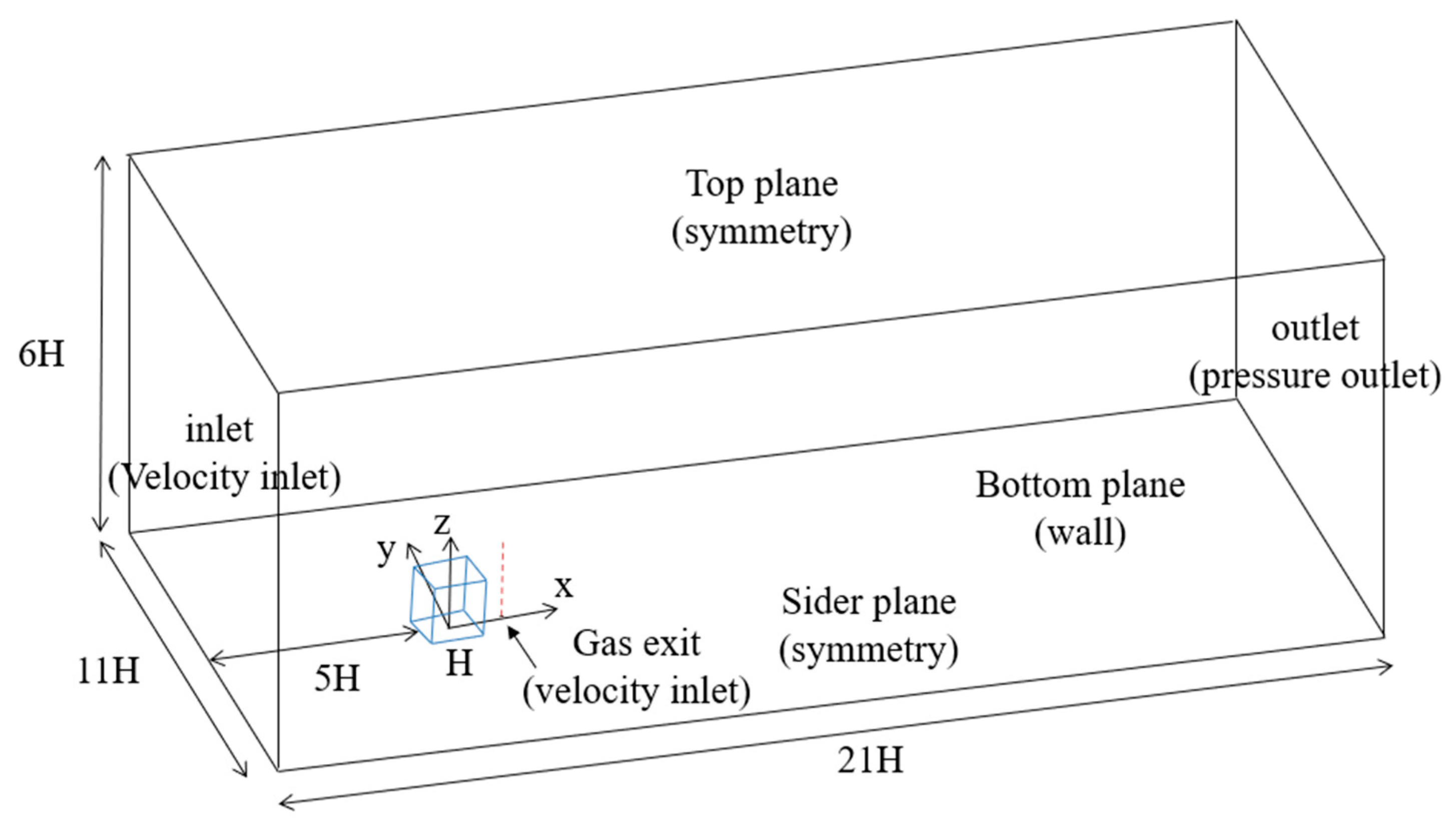
Numerical Method
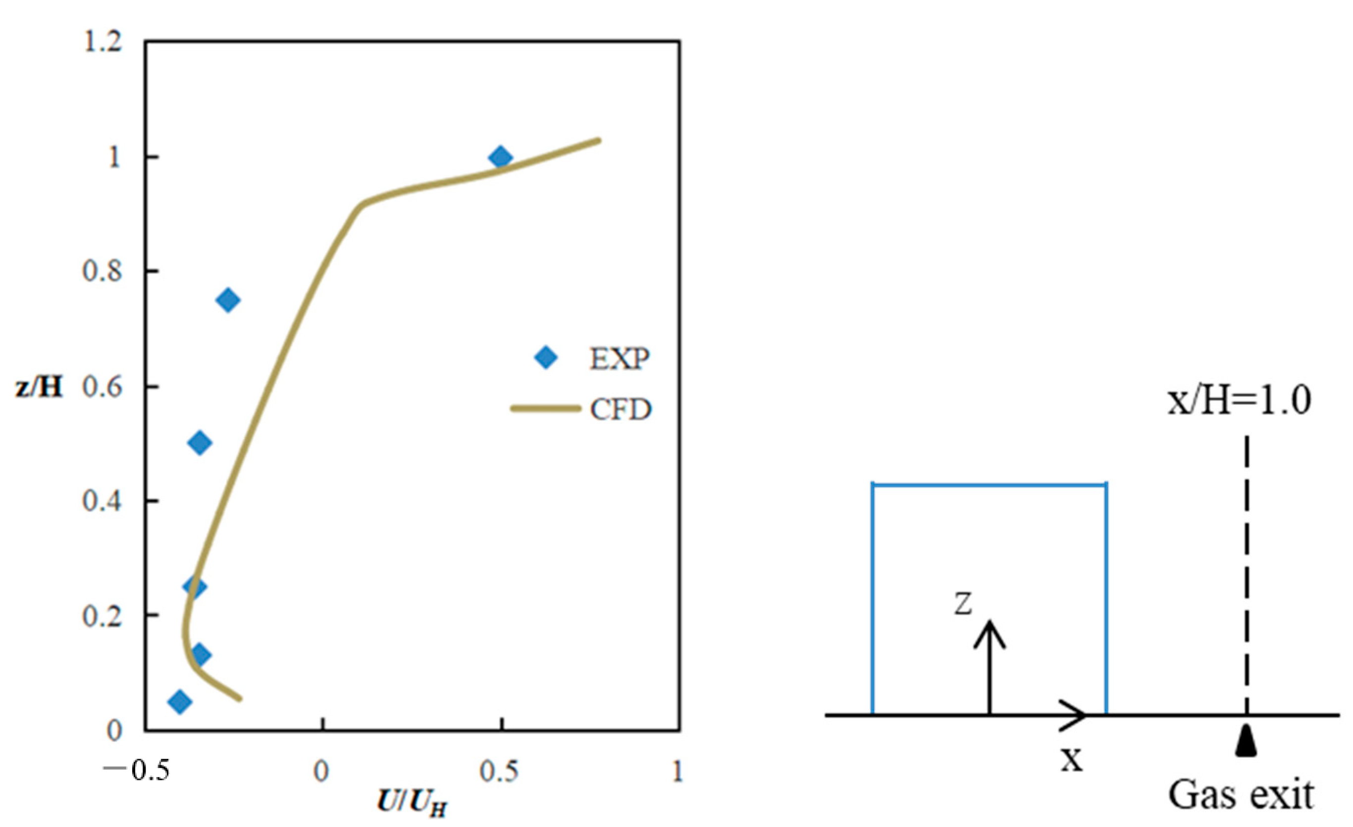
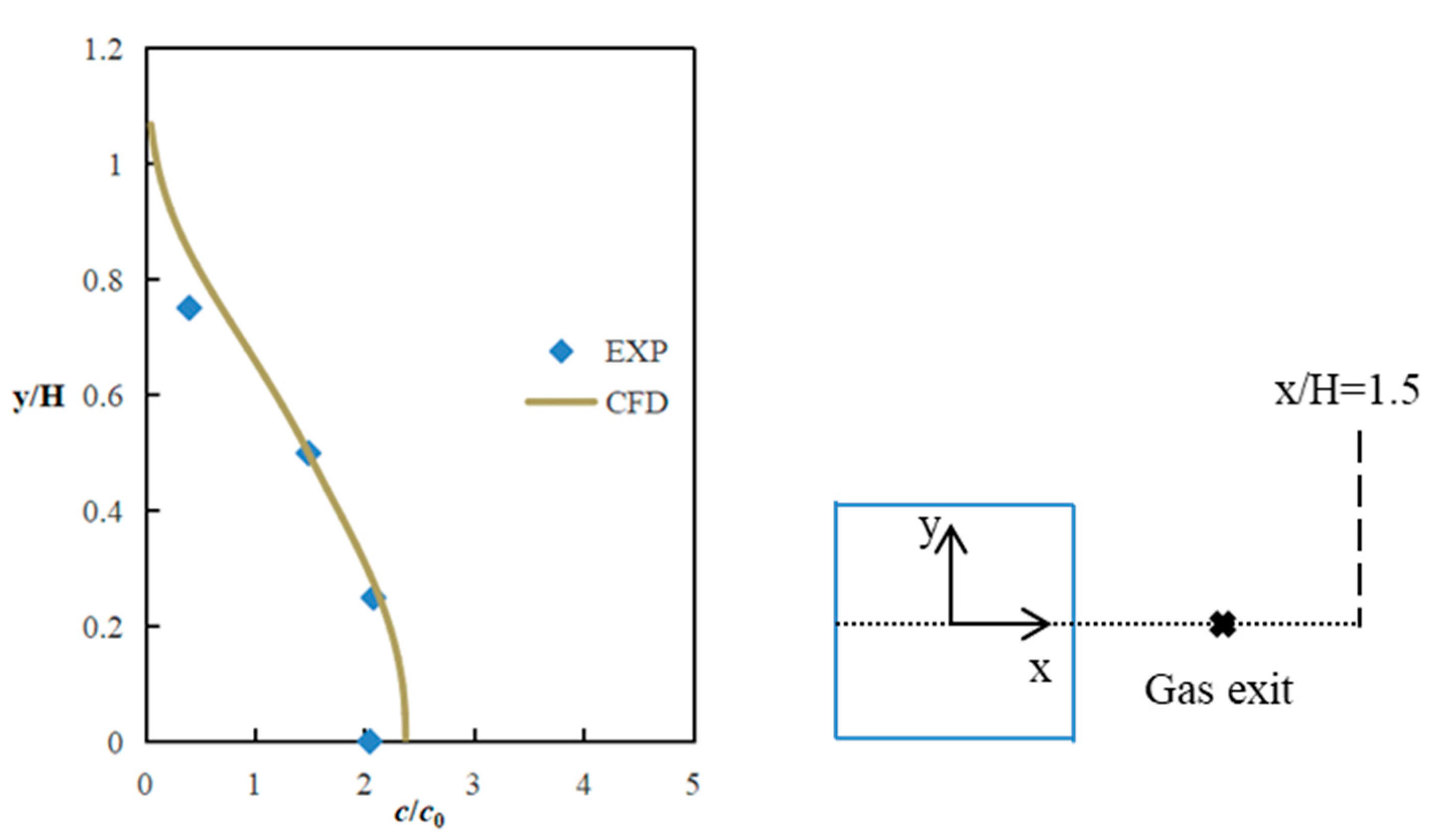
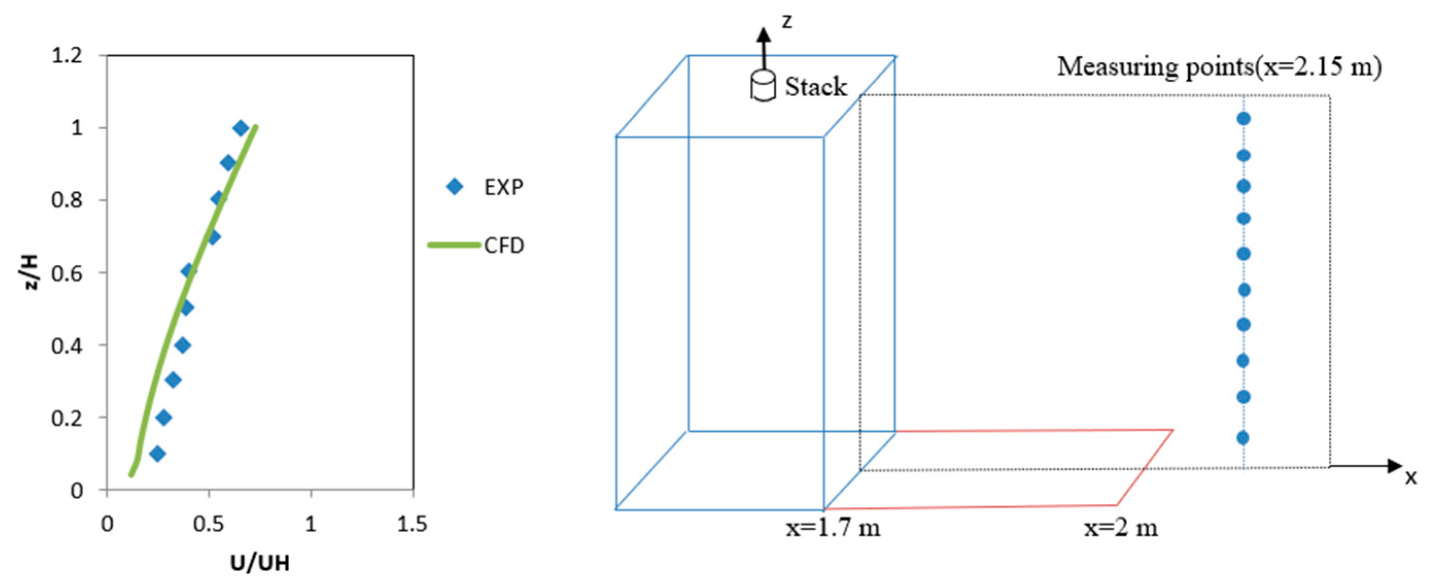
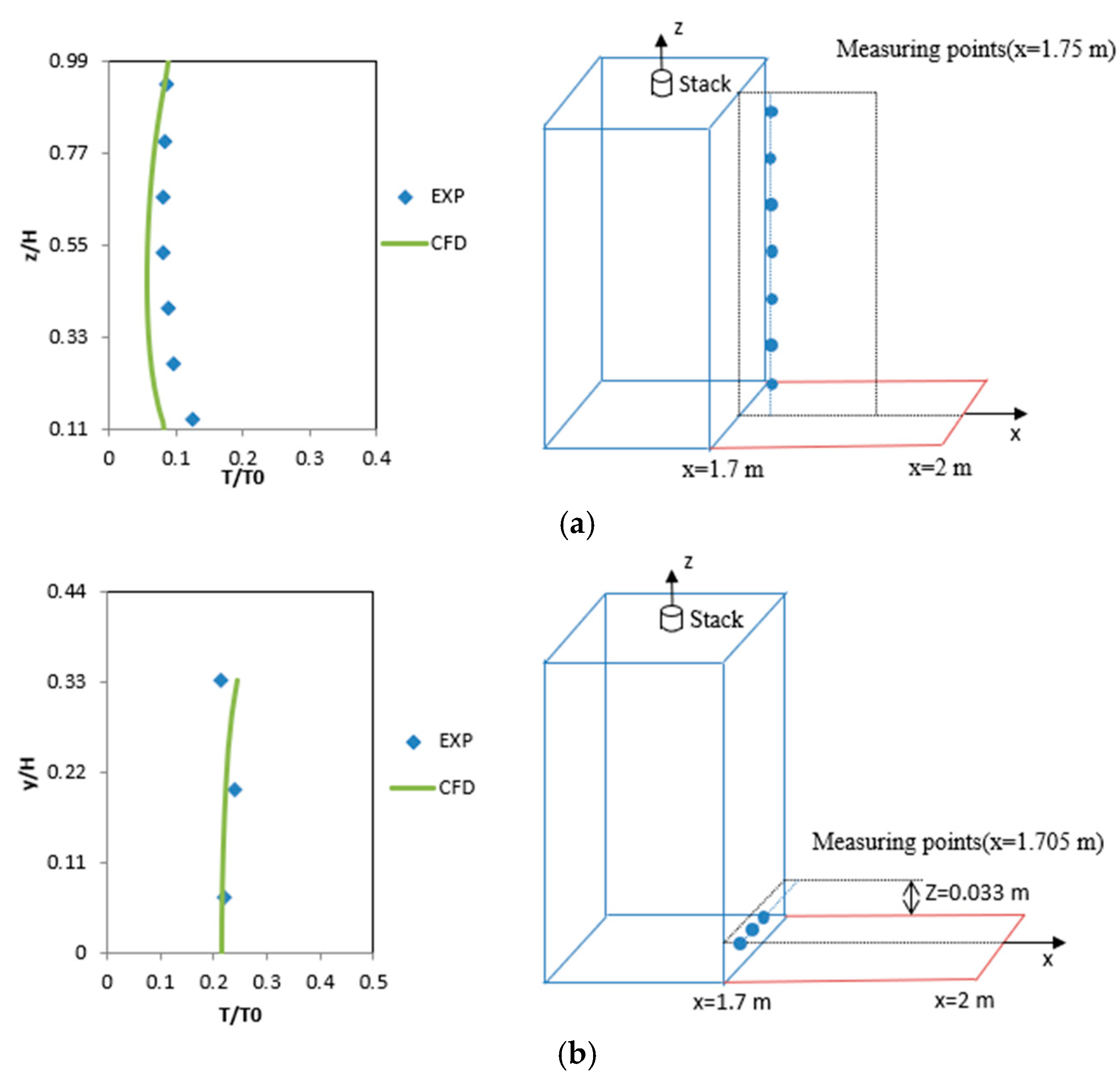
Validation of the Numerical Method
CFD Simulation Cases for Building the Fitting Formulas
2.1.2. Heating Building Simulation
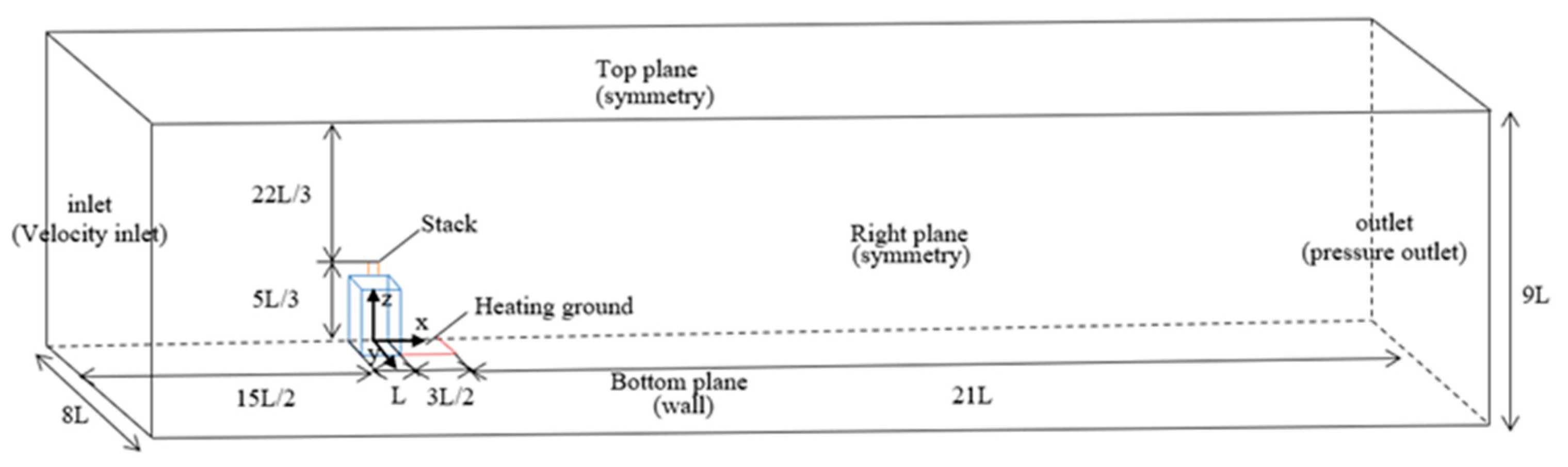
Numerical Method
Validation of the Numerical Method
Validation Cases for the Fitting Formulas
2.2. Response Surface Methodology
- (1)
- Experimental design. The relationship between dependent variables and independent variables is clarified according to the research purpose. The range of independent variables was determined. Then, appropriate methods are used to determine the permutations and combinations of the values of a series of independent variables.
- (2)
- Acquisition of response data. Response data are obtained through experiment or simulation.
- (3)
- Establishment of response surface model. The experimental or simulation results are used to fit to a suitable mathematical model, and the correlation coefficient of the model is determined by regression analysis.
2.3. Support Vector Machine
3. Results
3.1. Correlation of the Convective Heat Transfer Coefficients
3.2. Validation of the Fitting Formulas
4. Conclusions
Author Contributions
Funding
Institutional Review Board Statement
Informed Consent Statement
Data Availability Statement
Conflicts of Interest
References
- Na, R.; Shen, Z.G. Assessing cooling energy reduction potentials by retrofitting traditional cavity walls into passively ventilated cavity walls. Build. Simul. 2021, 14, 1295–1309. [Google Scholar] [CrossRef]
- Ahmadi, J.; Mahdavinejad, M.; Larsen, O.K.; Zhang, C.; Zarkesh, A.; Asadi, S. Evaluating the different boundary conditions to simulate airflow and heat transfer in Double-Skin Facade. Build. Simul. 2022, 15, 799–815. [Google Scholar] [CrossRef]
- Nardi, I.; Lucchi, E.; de Rubeis, T.; Ambrosini, D. Quantification of heat energy losses through the building envelope: A state-of-the-art analysis with critical and comprehensive review on infrared thermography. Build. Environ. 2018, 146, 190–205. [Google Scholar] [CrossRef] [Green Version]
- Nardi, I.; Paoletti, D.; Ambrosini, D.; de Rubeis, T.; Sfarra, S. U-value assessment by infrared thermography: A comparison of different calculation methods in a Guarded Hot Box. Energy Build. 2016, 122, 211–221. [Google Scholar] [CrossRef]
- Bouchair, A. External environmental temperature: Proposed new formulation. Build. Serv. Eng. Res. Technol. 2001, 22, 133–156. [Google Scholar] [CrossRef]
- McAdams, W.H. Heat Transmission; McGraw-Hill Kogakusha: Tokyo, Japan, 1954. [Google Scholar]
- Jürges, W. Der wärmeübergang an einer ebenen wand (heat transfer at a plane wall). Gesundh.-Ing. 1924, 1, 105. [Google Scholar]
- Sparrow, E.M.; Ramsey, J.W.; Mass, E.A. Effect of finite width on heat transfer and fluid flow about an inclined rectangular plate. J. Heat Transf. 1979, 101, 199–204. [Google Scholar] [CrossRef]
- Jayamaha, S.E.G.; Wijeysundera, N.E.; Chou, S.K. Measurement of the heat transfer coefficient for walls. Build. Environ. 1996, 31, 399–407. [Google Scholar] [CrossRef]
- Sturrock, N.S. Localised Boundary Layer Heat Transfer from External Building Surfaces. Ph.D. Thesis, University of Liverpool, Liverpool, UK, 1971. [Google Scholar]
- Ito, N.; Kimura, K.; Oka, J. Field experiment study on the convective heat transfer coefficient on exterior surface of a building. ASHRAE Trans. 1972, 78, 184–191. [Google Scholar]
- Nicol, K. The energy balance of an exterior window surface, Inuvik, NWT, Canada. Build. Environ. 1977, 12, 215–219. [Google Scholar] [CrossRef]
- Yazdanian, M.; Klems, J.H. Measurement of the exterior convective film coefficient for windows in low-rise buildings. ASHRAE Trans. 1994, 100, 1087–1096. [Google Scholar]
- Loveday, D.L.; Taki, A.H. Convective heat transfer coefficients at a plane surface on a full-scale building facade. Int. J. Heat Mass Transf. 1996, 39, 1729–1742. [Google Scholar] [CrossRef]
- Hagishima, A.; Tanimoto, J. Field measurements for estimating the convective heat transfer coefficient at building surfaces. Build. Environ. 2003, 38, 873–881. [Google Scholar] [CrossRef]
- Yamamoto, T.; Ozaki, A.; Kaoru, S.; Taniguchi, K. Analysis method based on coupled heat transfer and CFD simulations for buildings with thermally complex building envelopes. Build. Environ. 2021, 191, 107521. [Google Scholar] [CrossRef]
- Defraeye, T.; Blocken, B.; Carmeliet, J. Convective heat transfer coefficients for exterior building surfaces: Existing correlations and CFD modelling. Energy Convers. Manag. 2021, 52, 512–522. [Google Scholar] [CrossRef] [Green Version]
- Fakhim, H.A.; Zamzamian, K.; Hanifi, M. Investigating the Effect of Different Parameters on CHTC Using Wind-Tunnel Measurement and Computational Fluid Dynamics (CFD) to Develop CHTC Correlations for Mixed CHTCS. J. Mech. 2020, 36, 915–932. [Google Scholar] [CrossRef]
- Chen, S.; Mihara, K.; Wen, J. Time series prediction of CO2, TVOC and HCHO based on machine learning at different sampling points. Build. Environ. 2018, 146, 238–246. [Google Scholar] [CrossRef]
- Yi, Q.; Zhang, G.; Amon, B.; Hempel, S.; Janke, D.; Saha, C.K.; Amon, T. Modelling air change rate of naturally ventilated dairy buildings using response surface methodology and numerical simulation. Build. Simul. 2021, 14, 827–839. [Google Scholar] [CrossRef]
- Tominaga, Y.; Stathopoulos, T. CFD Simulations of Near-field Pollutant Dispersion with Different Plume Buoyancies. Build. Environ. 2018, 131, 128–139. [Google Scholar] [CrossRef]
- Mochida, A.; Tominaga, Y.O.; Murakami, S.; Yoshie, R.; Ishihara, T.; Ooka, R. Comparison of various k-models and DSM applied to flow around a high-rise building—Report on AIJ cooperative project for CFD prediction of wind environment. Wind. Struct. 2002, 5, 227–244. [Google Scholar] [CrossRef] [Green Version]
- ANSYS. ANSYS 19 Fluent Theory Guide; ANSYS: Canonsburg, PA, USA, 2018. [Google Scholar]
- Huang, Y.D.; Xu, N.; Ren, S.Q.; Qian, L.B.; Cui, P.Y. Numerical investigation of the thermal effect on flow and dispersion of rooftop stack emissions with wind tunnel experimental validations. Environ. Sci. Pollut. Res. 2021, 28, 11618–11636. [Google Scholar] [CrossRef]
- Vapnik, V. The Nature of Statistical Learning Theory, 2nd ed.; Springer: Berlin/Heidelberg, Germany, 1999. [Google Scholar]
- Hsu, C.W.; Chang, C.C.; Lin, C.J. A Practical Guide to Support Vector Classification. Dep. Comput. Sci. 2003, 106, 1396–1411. [Google Scholar]


| Wind Velocity Range | |||
|---|---|---|---|
| Flow regime | Natural convection | Mixed convection | Forced convection |
| Wind Velocity /m/s | Wind Direction Angle/° | Temperature Difference/K |
|---|---|---|
| 0.2 | 0 | 1 |
| 0.4 | ||
| 0.6 | 30 | 2 |
| 0.8 | ||
| 1 | 45 | 3 |
| 1.2 |
| Inflow Wind Velocity/m/s | Temperature Difference/K |
|---|---|
| 1.5 | 40 |
| 3 | 80 |
| 4.5 | 120 |
| Surface | Response Surface Model | R-Square | Predicted |
|---|---|---|---|
 Top side | 0.9619 | 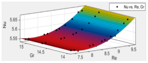 | |
 Windward side | 0.9978 | 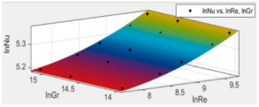 | |
 Lee side | 0.9789 |  |
| Surface | Response Surface Model | R-Square | Predicted |
|---|---|---|---|
 Lee side 1 | 0.7154 |  | |
 Lee side 2 | 0.9304 |  | |
 Windward side | 0.9411 |  |
| Surface | Accuracy | Best C, Gamma | Surface |
|---|---|---|---|
| Top side | 100% | 2, 2 |  |
| Windward side | 72.22% | 2, 8 |  |
| Lee side | 61.11% | 32, 0.5 |  |
| Surface | Accuracy | Best C, Gamma | Surface |
|---|---|---|---|
| Lee side 1 | 91.67% | 32, 0.5 |  |
| Lee side 2 | 86.11% | 2, 8 |  |
| Windward side | 98.61% | 8, 2 |  |
| Error | |||||
|---|---|---|---|---|---|
| CFD Simulation Value | RSM Fitted Value | SVM Fitted Value | RSM | SVM | |
| 3, 120 | 5.838 | 6.261 | 5.597 | 7.25% | 4.13% |
| 3, 80 | 5.867 | 6.260 | 5.584 | 6.70% | 4.82% |
| 3, 40 | 5.969 | 6.259 | 5.578 | 4.86% | 6.55% |
| 1.5, 120 | 5.767 | 5.736 | 5.759 | 0.54% | 0.14% |
| 1.5, 80 | 5.782 | 5.735 | 5.750 | 0.81% | 0.55% |
| 1.5, 40 | 5.664 | 5.734 | 5.739 | 1.24% | 1.32% |
| 4.5, 120 | 6.128 | 6.570 | 5.872 | 7.21% | 4.18% |
| 4.5, 80 | 6.113 | 6.569 | 5.858 | 7.46% | 4.17% |
| 4.5, 40 | 6.109 | 6.568 | 5.851 | 7.51% | 4.22% |
Publisher’s Note: MDPI stays neutral with regard to jurisdictional claims in published maps and institutional affiliations. |
© 2022 by the authors. Licensee MDPI, Basel, Switzerland. This article is an open access article distributed under the terms and conditions of the Creative Commons Attribution (CC BY) license (https://creativecommons.org/licenses/by/4.0/).
Share and Cite
Xue, X.; Han, S.; Guo, D.; Zhao, Z.; Zhou, B.; Li, F. Study of the Convective Heat Transfer Coefficient of Different Building Envelope Exterior Surfaces. Buildings 2022, 12, 860. https://doi.org/10.3390/buildings12060860
Xue X, Han S, Guo D, Zhao Z, Zhou B, Li F. Study of the Convective Heat Transfer Coefficient of Different Building Envelope Exterior Surfaces. Buildings. 2022; 12(6):860. https://doi.org/10.3390/buildings12060860
Chicago/Turabian StyleXue, Xiaotong, Shouxu Han, Dongjun Guo, Ziwei Zhao, Bin Zhou, and Fei Li. 2022. "Study of the Convective Heat Transfer Coefficient of Different Building Envelope Exterior Surfaces" Buildings 12, no. 6: 860. https://doi.org/10.3390/buildings12060860
APA StyleXue, X., Han, S., Guo, D., Zhao, Z., Zhou, B., & Li, F. (2022). Study of the Convective Heat Transfer Coefficient of Different Building Envelope Exterior Surfaces. Buildings, 12(6), 860. https://doi.org/10.3390/buildings12060860