A Novel Computational Approach for an Improved Expression of the Spectral Content in the Lower Atmospheric Boundary Layer

Abstract

The paper presents an innovative methodology for the simulation of incoming wind conditions in computational domains that use large eddy simulation (LES) for the evaluation of wind loads on low-rise buildings. Simulating the atmospheric boundary layer has proven to be a challenging process for computational wind engineering, especially to correctly introduce the fluctuations in the high-frequency spectral domain. Experiments in the Concordia University Building Aerodynamics Laboratory were carried out to estimate the evolution of turbulence features in the along-wind direction of a generic profile. Virtual probes were placed inside the computational domain to match the location of those in the wind tunnel and compare mean speed values, turbulence intensity, integral length scales, and spectral content. Synthetic methods were applied for the incoming wind velocity to estimate their capacity to capture the evolution of these turbulence features in the streamwise direction. The inability of these synthetic methods to represent the spectral domain, particularly for heights of interest for low-rise buildings, was examined, and the so-called dynamic terrain method in which velocity time histories are extracted from wind tunnel measurements and reconstructed to fit certain statistical parameters was implemented. The proposed method represents the frequency domain’s spectral content with good agreement with the theoretical von Karman spectrum and the experimental results. Advantages of the method include time efficiency and relative simplicity, which makes it attractive to the practitioners for the design of a neutral atmospheric boundary layer respecting the turbulent wind characteristics.

1. Introduction

Computational wind engineering has evolved from its “infancy” [1] in the past decades, due to the help of computational resources and the constant struggle of the community to evolve the current state-of-the-art tools. The advantages of adopting computational methods to evaluate fluctuating loads on building envelopes are significant, and their inclusion in code provisions is important. However, the correct expression of high-frequency fluctuations in the lower part of the atmospheric boundary layer, where most low-rise buildings reside, is necessary.

The proper definition of the inflow characteristics in turbulent terms is the best practice to create a more mature tool using computational fluid dynamics for structural design applications [1,2]. This understanding created a trajectory of research in the last few decades that focuses on numerical and/or analytical methods to generate atmospheric boundary layer (ABL) turbulent flow fields to be introduced as inlet conditions in large eddy simulation (LES). There are two categories of methods in this respect: the recycling methods and the synthetic methods. In the first category, an initial computational domain with cycling boundary conditions is used to re-circulate the inflow velocity components and generate “natural” random variations with the resulting velocity fluctuations to be subsequently inserted in the primary computational domain where the building resides. Studies focusing on these methods have succeeded in generating an appropriate turbulent field [3,4], but guidelines for the properties of the initial computational domain and relations for its interaction with the turbulence length scales have proven challenging and case oriented. The lack of generalization in these methods and the aforementioned difficulties can be avoided by using the synthetic approach.

Synthetic methods can be distinguished into three sub-categories; synthetic eddy methods, random flow generators, and digital filtering. In the first sub-category, fluctuations are generated by superposing natural vortices to mean velocity [5,6,7]. As a method, it has the advantage that turbulent length scales can vary with height, but the divergent-free condition is not guaranteed; thus, unphysical pressure fluctuations will be generated in the building envelope, making even the latest versions of the method inappropriate for building design.

Random flow generators use the summation of sinusoidal waves with a range of amplitudes, frequencies, and phase shifts [8,9]. Their application has seen great improvements in the last few years when the accurate spectral representation was introduced, making them appropriate for use in ABL flows [10,11,12,13]. Melaku et al. [14] introduced a solution process based on Deodatis [15] and the inverse Fourier composition to generate the final inflow time series. The algorithm was implemented in OpenFOAM for general use and was tested for the purposes of the study, although results indicated that more calibrations are necessary to achieve consistent velocity distributions for rough terrain.

Finally, the third sub-category has shifted most of the attention in the past decade, due to the accuracy of results not only for the velocity turbulent characteristics [16,17], but also for the accurate representation of the pressure contour [18] for building design. Kim et al. [19] first introduced some significant modifications in previous works [16,20], which regard the correct mass flux and the divergent-free condition by introducing a correction in the incoming velocity to a plane parallel to the inlet, thus removing the non-physical pressure that appears in the computational domain. A reconstruction of the PISO algorithm was necessary, and the new version is available for use in the OpenFOAM package. These improvements by Kim et al. [19] was further elaborated by Patruno et al. [21]. The synthetic digital filter method (SDFM) technique was chosen because of its accuracy and the fact that its application is well calibrated and open for use by practitioners in OpenFOAM.

Comparative studies of the methods are available in the literature [4,22,23,24,25,26], and their close attention led to two main hindrances and vital gaps. The first regards the second-order statistics of velocity, the turbulence intensity, and its evolution in the computational domain. Tieleman [27] compared experimental results with full-scale measurements and concluded that the turbulence intensity at the building height is the most important factor to match the pressure values in the building envelope, producing an accurate design for low-rise buildings.This proves the necessity of accurate turbulence intensity representation in wind tunnel tests and computational procedures via LES that use synthetic turbulence at the inlet boundary, more precisely, the turbulence intensity at the location of interest, where the test model resides. Therefore, it is crucial to express the turbulence decay accurately in computational procedures. In order to maintain the turbulent character of the flow, when using the random flow generation techniques, in the distance between the inlet and the location of interest, Ricci et al. [28] included roughness elements in the computational domain, and Guichard [29] recalculated the inlet intensity. Lamberti et al. [17] concluded a parametric study to optimize the Reynolds stress tensor that is used as the input by the algorithm, to achieve a target turbulent vertical flow distribution at the position of interest while using the SDFM. In the present study, the target is not to calibrate the turbulent intensity in the location of interest, but to quantify the capacity of the various methods to estimate this decay as measured in the wind tunnel. For that reason, the turbulence decay of a generic profile was measured in the Concordia University Building Aerodynamics Laboratory, as will be presented in detail in Section 2 of this paper.

The second and most important hindrance regards the spectral representation of the synthetic methods in the lower part of the ABL. This part interacts directly with low-rise structures; thus, it is essential to create computational tools capable of representing it in detail. In all aforementioned works that apply synthetic approaches, the spectral content in the domain’s high-frequency part is underestimated compared with the theoretical von Karman spectral distribution and wind tunnel results. In theoretical terms, fluctuations in the high part of the frequency domain are closely correlated with peak (design) values; therefore, it is important to represent them accurately. Mooneghi et al. [30] proposed an analytical method for estimating peak values that match full-scale data, depicting this high part of the spectrum accurately, proving the advantages of properly expressing these high-frequency/small-scale fluctuations. The computational procedures proposed in this paper refer to directly applying wind tunnel velocity time series, as time-varying inlet conditions in the virtual wind tunnel in order to construct a boundary layer that respects the spatial coherency of the turbulence features measured in the experiments in the entire frequency domain. In reference [31], the authors concluded a similar approach for the inlet conditions regarding the pollutant dispersion in a street canyon and introduced an improved SIMPLE algorithm to better calculate the time-dependent transitions. The direct and dynamic terrain methods were established to tackle the issue of spectral representation and will be presented in detail in Section 3 and Section 4.

2. Experimental Procedure

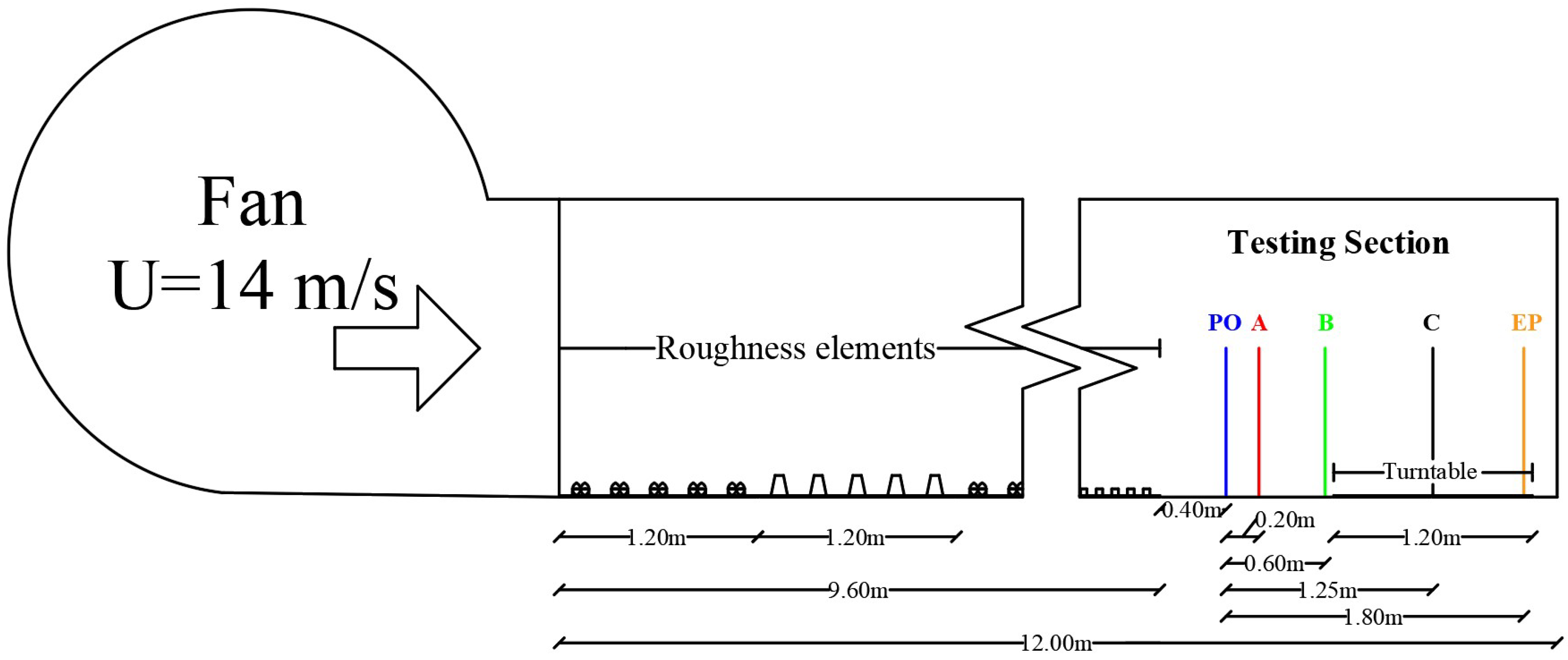
The Concordia Wind Tunnel was fabricated in 1981 and calibrated to represent a scaled atmospheric boundary layer [32]. It is an open return circuit wind tunnel, 12 m long and 1.80 m in width. The height of the tunnel is adjusted according to the selected terrain exposure and can range from 1.40 m to 1.80 m. The maximum velocity that can be reached by the fan is 14 m/s, a value that was used for the experiments of the study. Velocity time series with a range of 32.7 s were extracted from a probe, whose location can be selected manually in the transverse and longitudinal direction. The time series is large enough to ensure a stationary signal.

Traditionally, wind tunnel velocity measurements are extracted for the location of interest, where the building will reside. In the present study, the target is to tune the wind tunnel with a virtual wind tunnel that uses LES for the calculation of the velocity time series. For that reason, more than one location of interest was selected, to evaluate the evolution of the turbulent features in computational methodologies with various assumptions for the incoming flow at the inlet boundary. Most low-rise structures reside in locations where open terrain conditions are impossible to achieve, while rougher terrains usually create more conservative conditions for the design values on the building envelope; thus, safety and a more realistic approach accompany them. In order to include rough terrain conditions and quantify the spatially developing features of the ABL flow, the configuration in Figure 1 was established in the wind tunnel.

The wind tunnel carpet consists of eight blocks of individual roughness elements with a length of 1.2 m each. First, the higher roughness elements available are placed to generate turbulent features near the fan and then the shorter ones, with a distance of 0.4 m from the first measurement point to avoid wake region effects. The total length of the roughness elements was calculated to be 9.60 m. Due to this formulation, rough terrain conditions are present in the first location PO for the mean speed and the turbulent intensity. The spatial coherency of these turbulent structures downstream, without roughness elements, is of great interest for computational comparisons. The rest of the locations of interest consist of point A, point B, point C, where the location of the testing model is, and finally, the endpoint EP. The dimensions of the testing section from point PO to EP are consistent with the computational domain that is presented in Section 3. Velocity time series were extracted for the first 0.45 m of the layer, using 19 independent heights. A scaling factor of 1/400 was adopted for experiments in the wind tunnel [32]; thus, the first 180 m of the ABL were simulated in full-scale. Low-rise buildings interact with the lower part of the layer; thus, results for the first 80 m were considered important and are presented in this paper, as extracted from the first 14 points.

In

Table 1. Mean velocity of generic profile at selected locations according to power and logarithmic laws.

Location	$\mathit{\alpha }$	Experimental ${\mathit{z}}_0$ (m)
PO	0.24	0.51
A	0.21	0.24
B	0.18	0.1
C	0.14	0.04
EP	0.12	0.0034

, the exponents ($\alpha$) are presented according to the power-law (Equation (1)), where z is the distance from the ground and $z_{ref}$ the reference height at 0.20 m (or 80 m full-scale). The logarithmic law (Equation (2)) is used to calculate the roughness length ($z_0$), where u* is the friction velocity calculated as 0.7 m/s and k is the von Karman constant. The values were calculated by linearizing the corresponding equations and considering points residing above 10 m. Results state that as the wind flow progresses in the windward direction (points A and B), the mean distribution moves towards the open terrain. At point C, the values reach a classic open terrain distribution, which is used in the wind tunnel, with an exponent of 0.14. Finally, the vertical distribution of the mean speed resembles an open profile with exponent 0.12 at EP. The corresponding values of the roughness height $z_0$ agree with provisions established in ASCE 49-12, when compared with the power-law exponents $\alpha$.

$$U\left(z\right)=U_{ref}·{(z/z_{ref})}^{\alpha },z_{ref}=0.20\mathrm{m}\left(80\mathrm{m}\right)$$

(1)

$$U\left(z\right)=\frac{u_{*}}{\kappa }·ln(z/z_0),u_{*}\simeq 0.7\mathrm{m}/\mathrm{s}$$

(2)

The above experimental procedure refers to sudden variations in the terrain conditions and was not the only one that was tested. A smoother rough terrain was also established in the wind tunnel where the mean velocity decay was found to range from $z_0$ = 0.37 at PO to $z_0$ = 0.0033 at EP. An open terrain was also tested (no roughness elements), where the decay of the mean speed was calculated to vary from $z_0$ = 0.06 at PO to $z_0$ = 0.003 at EP. The aerodynamic interference in the proximity of the roughness elements was found to dissipate from the region of PO and C, which is a distance of great interest for equivalent computational domains. The target of the study is to evaluate the mitigation of these effects in computational procedures and establish the capacity of various inlet conditions to predict the most sudden variations in the mean and turbulence intensity profiles with height. It can be considered less challenging to evaluate in terms of decay open or smoother terrains than the one selected, and the computational methods presented later in the paper would be equally applicable. From a realistic point of view, this configuration tries to evaluate how the above decays will interact with the location of interest when conducting experimental procedures for rough terrains. The distance of 1.65 m between the last roughness element and the location of interest C seems to be large enough to decay the profiles and generate the generic profile of interest for the study.

The inner boundary layer that is generated due to roughness discontinuity has been a sensitive topic of research during the last few decades. This is the height at which the new surface roughness affects the mean flow. It is defined downwind from the discontinuity and increases with the fetch until the entire boundary layer adjusts to the new roughness length. Based on Deaves [33] and Wood [34], the height of the inner boundary layer ${\delta }_i$ can be estimated by using the empirical equations displayed in Figure 2, where x is the distance downstream of the first measurement point. The experimental results of this article seem to agree more with the proposed equation from Wood [34], since a larger height of the layer is in equilibrium with the open terrain—see the values of $z_0$ in Table 1. It is important to mention that the procedures for the calculation of $z_0$ based on experimental data can only be approximate, due to the nature of this parameter. This is also supported by observing the structure of wind codes and standard provisions in this matter, where ranges of $z_0$ are provided in lieu of specific values, and by the large deviation established by using the two different equations in Figure 2. Reference [35] provides further information about the trajectory of research on the topic of the inner boundary layer height in surface roughness transitions for wind flow applications.

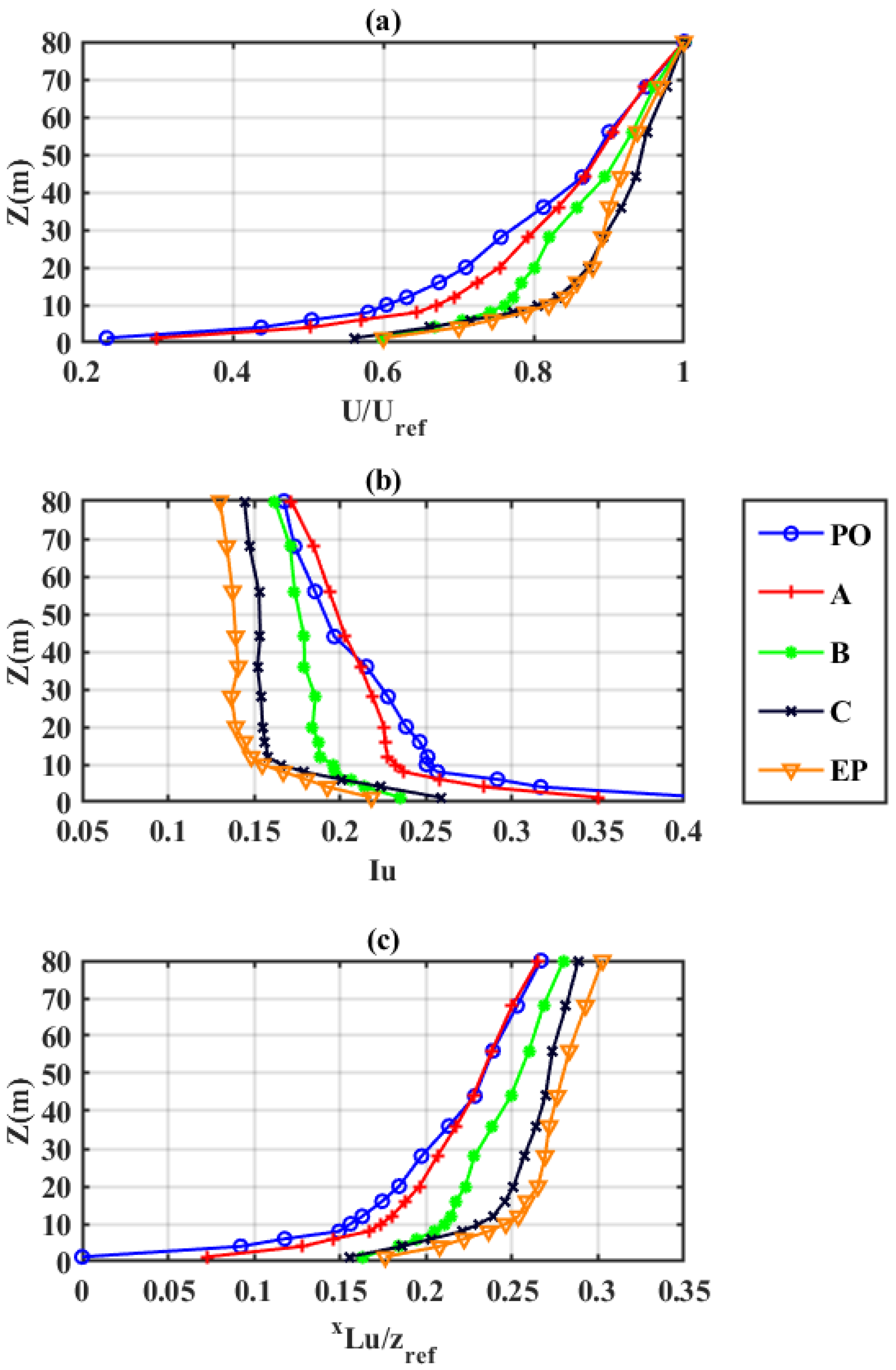
In Figure 3a, the mean values of the velocity are presented for the five locations that were selected. Values were normalized with the velocity of each point at a reference height of 80 m. Figure 3b presents the turbulence intensity values for the first 80 m of the layer in full-scale. As can be seen, the turbulence intensity follows a similar pattern as the mean values; the transition from rough to open terrain is again evident. At points A, B, and C and EP, the profiles are affected by the incoming flow at PO, and the turbulence intensity distributions have a strong turbulent remaining content when they were compared with provisions that refer to the corresponding mean value data. For example, at point C, although the mean values correspond to an open profile, the turbulence intensity distributions denote a rougher exposure; thus, the profiles are defined as generic (or decaying). Finally, in Figure 3c, the integral length scale in the longitudinal direction is displayed. The variations in the length scale follow those in the mean values since Taylor’s hypothesis [36] was used for its calculation.

When physical obstacles are not present (roughness elements in the wind tunnel), the kinetic energy near the ground transforms into thermal energy, and turbulence decays until an equilibrium state is reached. In computational domains, simulating physical obstacles increases the cost and makes the results case-oriented (number of elements, turbulence statistics, etc.); thus, open terrain conditions are usually assumed between the inlet plane and the building location. The range of turbulence decay in these regions (from PO to C) depends primarily on the turbulence intensity at the point of origin.

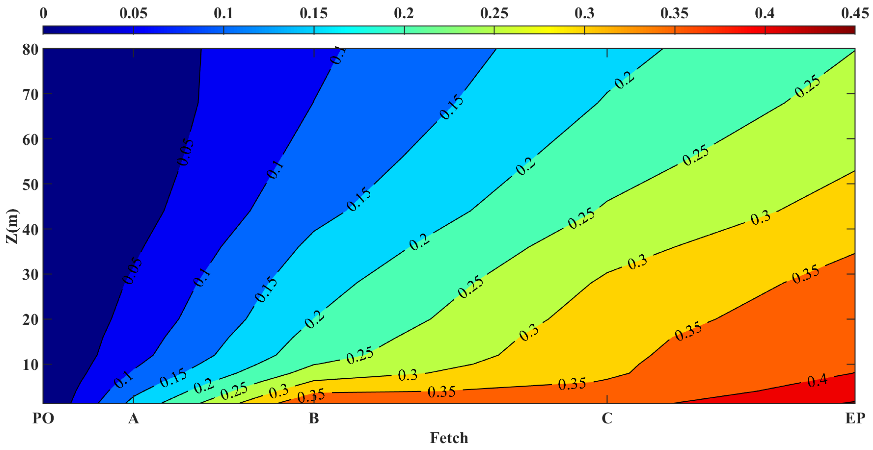
In Figure 4, the turbulence decay of the generic profile is presented, as defined in Equation (3), where $I_{i,z}$ is the turbulence intensity at point i, measured at height z. In point A, the decay starts from the ground with a value of 15%, and at the top 80 m, the decay is decreased to a value of 5%. At B, decay ranges from 35% at the bottom of the layer to 10% at the top. At the location of interest, C, decay starts from almost 40% and varies until 20%, and finally, at EP, 40% decay is measured near the ground and 25% at the top. These data depict that the turbulence decay follows a proportional trend with the fetch and it is more dominant in the first 40 m of the layer since the highest values reside until this height. The inherent difficulties in conducting accurate low-rise building design from experimental procedures to match full-scale conditions are strongly related to the turbulence decay in the first 40 m of the ABL that interacts directly with the structures.

$$T.D{.}_{i,z}=\frac{I_{\mathrm{PO},z}-I_{i,z}}{I_{\mathrm{PO},z}},i=\mathrm{PO},\mathrm{A},\mathrm{B},\mathrm{C},\mathrm{EP}$$

(3)

Wind tunnel practices have been established for many decades in the wind engineering community and are trusted for the safe and accurate design of low-rise buildings. Wind tunnel results and computational resources need to go hand in hand until the former are utilized regarding the evolution of the turbulent features in the streamwise direction to optimize/calibrate the latter in order to calculate correctly the incoming wind loading that will interact with the building of interest. Special attention to these features is necessary at the building height.

3. Synthetic Turbulent Flow Generation and Direct Method

The most appropriate way to establish computational practices for wind engineering is their comparison with wind tunnel results. For this comparison to be meaningful, a computational domain that is identical to the testing section in the wind tunnel was generated and used for all inlet methods. LES was selected for the numerical solution of the Navier–Stokes equations, and the main numerical features were kept intact during the parametric study to emphasize the differences only due to the inlet boundary conditions applied. The target results regard turbulence intensity, integral length scales, and spectral content in various heights of the ABL.

LES consists of one of the most trusted tools for simulating wind flows in the atmospheric boundary layer since it combines the apposite level of accuracy with manageable computational cost. The level of accuracy has proven to be superior to RANS turbulent models [37,38] because LES use spatial instead of time averaging. By spatially filtering the calculated values, a direct solution strategy is employed for the turbulent structures with a size larger than the filter size, while the subgrid ones are approximated with the subfilter model. For that reason, LES has the capacity to capture sudden deviations in the flow, making it an ideal design tool for calculating numerically the fluctuating wind loads on building envelopes. After the filter is applied, the Navier–Stokes equation takes the form presented in Equation (4), where $\overline{u}$ is the averaged velocity, $\overline{p}$ is the pressure, v is the molecular viscosity, and $v_t$ the eddy viscosity.

Small-scale eddies reach equilibrate states via strong nonlinear patterns that can be estimated by various subgrid-scale (SGS) models. The constant coefficient Smagorinsky model was the first to establish these patterns by an eddy viscosity model [39], which was later improved with the use of a damping function to better establish near-wall effects [40], and by Germano et al. [41], where the dynamic Smagorinsky models were introduced. Another approach that provided promising results to express the wall behavior in unsteady flows is based on the velocity gradient. The Wall-adaptive local eddy-viscosity (WALE) model, which belongs in this family, was chosen for the study, which regards Equations (5)–(9) to calculate the eddy viscosity $v_t$, where V is the volume of the cells and $C_w$ a model constant with a value of 0.325. More information about the theoretical aspect of the subfilter model can be found in Nicoud et al. [42]. A more robust model was recently proposed by Shui et al. [43] that might improve even more the accuracy of unsteady flows in the lower atmospheric boundary layer.

$$\frac{\partial \overline{u}}{\partial t}+{\overline{u}}_j\frac{\partial {\overline{u}}_i}{\partial x_j}=-\frac{1}{\rho }\frac{\partial \overline{p}}{\partial x_i}+\frac{\partial }{\partial x_j}([\nu +{\nu }_t]\frac{\partial {\overline{u}}_i}{\partial x_j})$$

(4)

$${\nu }_t={\Delta }_s^2\frac{{(S{}_{ij}^{d}S{}_{ij}^d)}^{3/2}}{{({\overline{S}}_{ij}{\overline{S}}_{ij})}^{5/2}+{(S{}_{ij}^{d}S{}_{ij}^d)}^{5/4}}$$

(5)

$${\Delta }_s=C_w{V}^{1/3}$$

(6)

$$S_{ij}^d=\frac{1}{2}({\overline{g}}_{ij}^2+{\overline{g}}_{ji}^2)-\frac{1}{3}{\delta }_{ij}{\overline{g}}_{kk}^2$$

(7)

$${\overline{g}}_{ij}=\frac{\partial {\overline{u}}_i}{\partial x_j}$$

(8)

$${\overline{g}}_{ji}^2={\overline{g}}_{ik}{\overline{g}}_{kj}$$

(9)

In Figure 5, the computational domain is presented that was used for all simulations of the study. The dimensions of the domain are consistent with the works by Ricci et al. [28] and Tominaga et al. [44] for the future inclusion of a low-rise building located at C, with full-scale dimensions b × d × h = 16 × 24 × 8 m. Symmetry conditions were applied to the sidewalls and the top wall, Neumann conditions of zero gradient for the outlet, and a solid wall in the ground to simulate the carpet in the wind tunnel. Dirichlet conditions were applied at the inlet plane and depend on each method that was tested. The wall model used for the estimation of the velocity in the first computational cells above the ground is the same as RANS analysis [17]. A second-order implicit numerical scheme was selected for the solution of the unsteady term; a second-order scheme was used for the gradient and divergent terms; a second-order unbounded and conservative scheme were used for the Laplacian terms. The PIMPLE algorithm in the OpenFOAM environment was employed for the solution of the system of equations.

The computational grid consists of polyhedral cells and was generated by dividing the computational domain in each direction. An excessive mesh (Grid 3) of 5.5 million cells was constructed by dividing the domain into 190, 225, and 128 cells in the x, y, and z directions, correspondingly, which was reduced to 3.7 million cells (Grid 2) by changing these values to 170, 200, and 110, correspondingly. Finally, a mesh of 2.6 million elements was adopted (Grid 1) by reducing the above values even further to 150, 180, and 98. Grid 1 was further parameterized by augmenting the number of cells in the x-direction from 150 to 200 and 300 since the streamwise direction can be considered more critical, but negligible variations were noticed. A denser mesh was selected near the ground in the z-direction and in the inlet plane in the x-direction in all cases, with a uniform expansion rate. The grid sensitivity study was conducted in terms of mean speed, turbulence intensity, and the Reynolds stress tensor in the streamwise direction between Grid 1 and 2 for a specific case and between Grid 1 and Grid 3 for another one. The comparisons proved that the mean error in the location of interest, C, is below 4%; thus, Grid 1 was chosen since it is the target of the study to establish inlet conditions for coarse computational domains, with less than three million elements.The time step of the analysis was also optimized by using an adjustable time-step algorithm according to a maximum value of CFL. For all results, CFLmax = 0.2 and CFLmean = 0.04 were used. As seen in Figure 5, virtual probes were inserted in the computational domain in the exact locations where the experimental measurements were drawn. Time series extracted from the computational domain match the experimental ones in terms of frequency and total duration.

The scope of the article is to follow the latest trend in the field toward defining LES as a computational design tool for structural purposes. CFD is a tool that can be manipulated easily; thus, it is important to create common ground and provisions to tune it to the wind tunnel practice. This tuning process has already started for some computational aspects such as the computational domain size, mesh size, numerical schemes for spatial and time derivatives, convergence criteria, divergent-free assumptions, time-step optimization, and wall boundary conditions. Each of these parameters introduces a level of inaccuracy in the system, but a parameter that seems to play a fundamental role in the proper simulation of the ABL is the inlet conditions. Calibrating them accurately with computational resources might prove beneficial for the target of computational wind engineering. Selecting low-rise buildings for that calibration seems the most natural first step because the first meters above the ground are the most difficult to simulate since the inherent turbulent features are strongly influenced by the solid boundary.

The first method to generate a turbulent atmospheric wind flow is the SDFM technique, established by Kim et al. [19] and last innovated by Lamberti et al. [17]. The method needs three sets of input information at the inlet plane. The first one regards the mean speed profile in the vertical direction, where the data from the wind tunnel in PO location were selected, as presented in Figure 3a. The second one is the Reynolds stress tensor, and it consists of a 3 × 3 matrix for each of the 19 vertical locations, which was calculated by the variance of the time series. The final input regards a uniform value for each one of the nine independent integral length scales, which corresponds to a 1 × 9 matrix. These values were chosen by calculating the nine independent time scales from the autocorrelation function and multiplying them with the mean velocity in the streamwise direction, by adopting Taylor’s hypothesis [36]. Further details regarding the sensitivity of this matrix in the generation of the target turbulence features can be found in Laberti et al. [17]. The values were compared with theoretical standards found in Simiu et al. [36] and were proven adequate. In that way, the turbulence that is generated and inserted into the domain should match the one measured at the PO location in the wind tunnel.

The second method in the first leg of the parametric study is the direct approach. In this technique, the extracted velocity time-series from the wind tunnel in location PO are introduced directly into the domain. The frequency of the probe measurements is 1000 Hz; thus, a time history of 0.001 s was constructed for each of the 19 points for the three velocity components and introduced into identical locations in the inlet boundary. The signals were divided into five segments, and their stationarity was confirmed. The first segment was used for the direct method with a range of 6.6 s. Transverse variations of the velocity profile were not considered, so a uniform across-wind profile was generated. Since the time series were applied directly to the inlet plane, turbulence features were developed rapidly in the computational domain, and the distance between the inlet and location of interest was satisfactory as the results of the turbulence statistics proved. To establish the accuracy of each method, focus was given to points PO and C, where the turbulence intensity and turbulence length scale were compared with experimental results. Finally, spectral representation was calculated from the two methods and compared with the wind tunnel and the theoretical von Karman spectrum for three heights of the layer. Mean velocity distributions were also examined, but the deviations that were noticed with fetch were closely related to the experimental results; thus, they were not included.

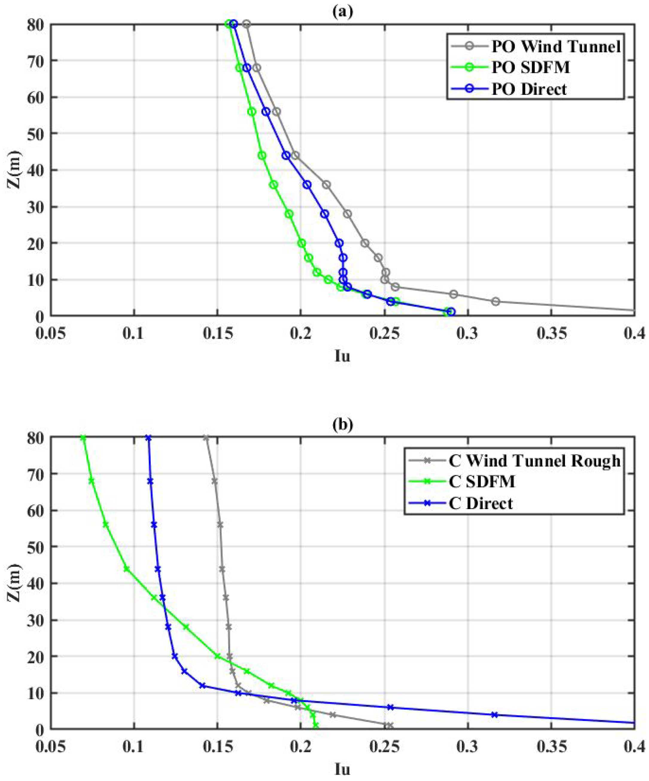
In Figure 6, the turbulence intensity profiles are depicted as calculated from the SDFM and direct method for PO and C. The turbulence intensity at PO is slightly underestimated by both methods for the first 80 m, while the calculated numerical distributions in the first 10 m are identical. At point C, the direct method provides superior results to the SDFM above 30 m. The trend of the SDFM results for the first 30 m are closely related to the experimental data, although the total decay is overestimated. Similar results can be found in Lamberti et al. [17], where the kinetic energy decays to values of 40% after 1 m. In reference [5], turbulence decay was also examined and a general conclusion was stated that this method overestimates the decay from inlet to outlet. Similar problems were reported in Guichard [29], where the random flow generation method by Yan et al. [22] was used. The issue of overestimating the turbulence decay is also spotted in the direct method, although the results are closer to the experimental ones and follow the same trend above 10 m. It is important to mention that above 80 m, the correlation of the results stays the same.

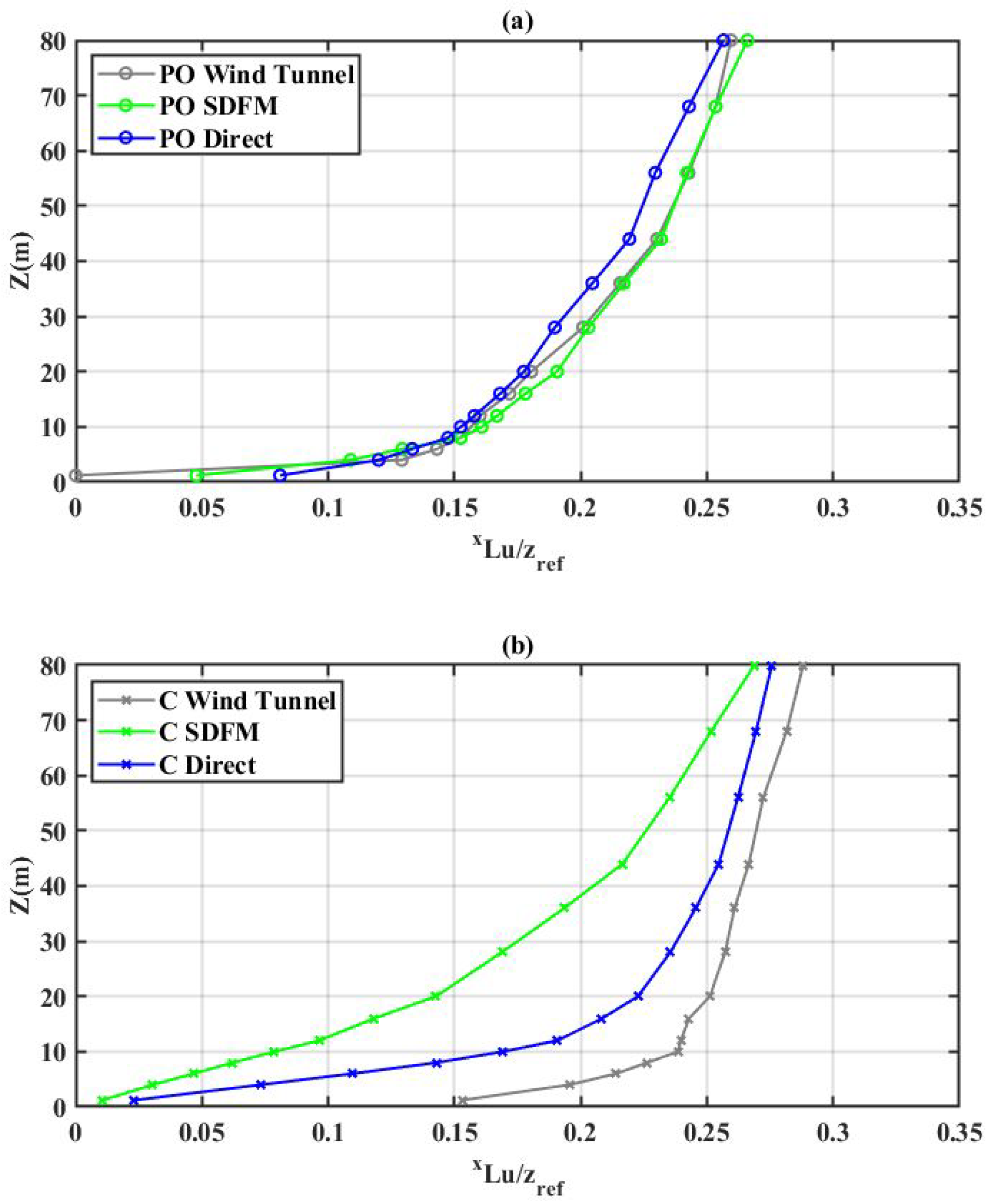
Integral length scales are compared in Figure 7 at PO and C. At PO, it is clear that both methods agree with the experimental results that were used to calculate the input parameters. At C, the SDFM seems to underestimate the turbulence length scale closer to the solid boundary and the direct method gives a small underestimation for the first 40 m of the layer. At higher heights, the distribution is perfectly matched with the experimental results, which indicates that a more accurate wall model might be needed. Alternatively, a larger fetch between the inlet and the point of interest [25] might be more appropriate to reach a more reliable ABL when using synthetic methods.

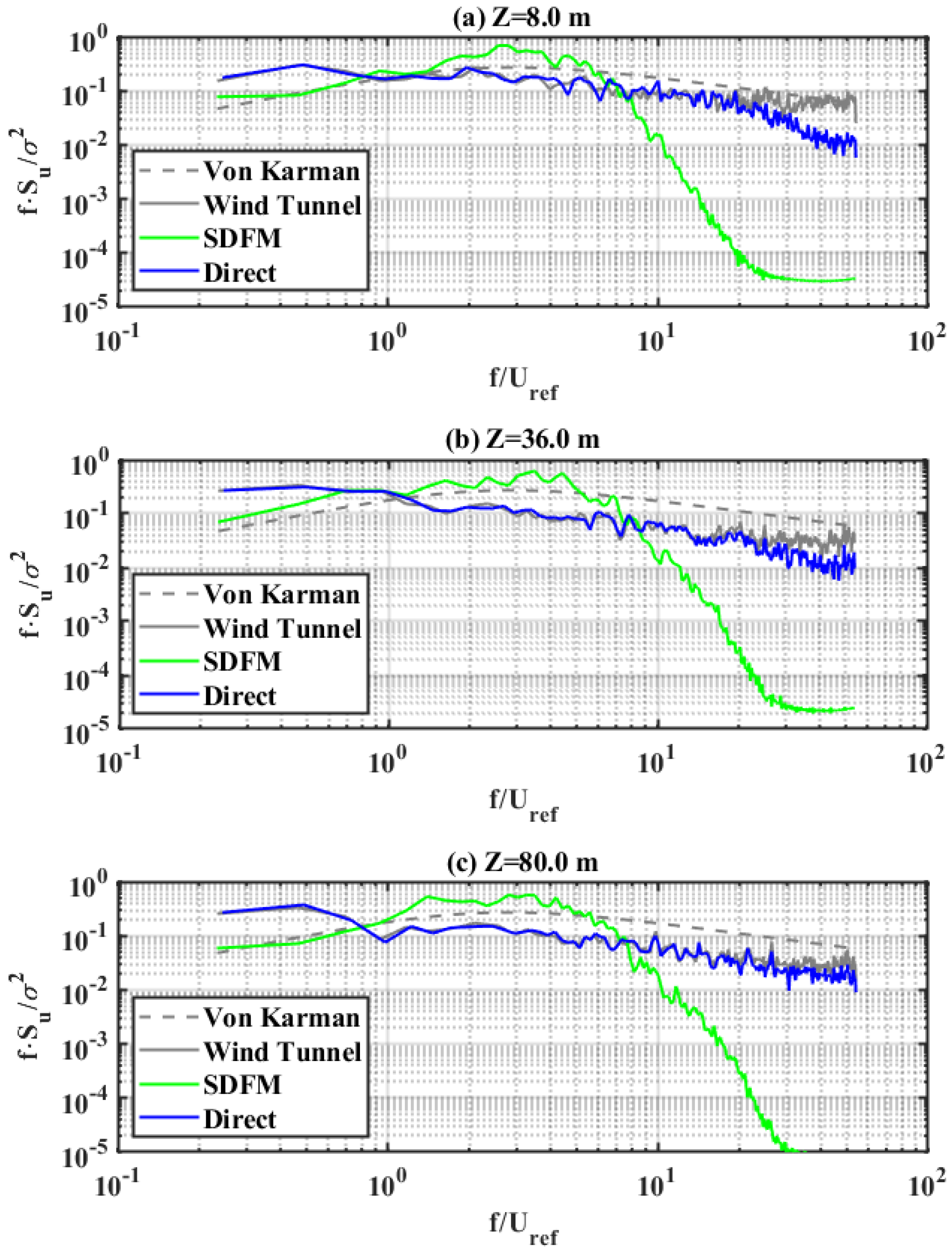
Regarding the spectral content of these methods and those calculated by the experiments and the theoretical von Karman (Equation (10)), in the longitudinal direction, three heights of the layer were examined: the first at 8 m in full-scale, the second at 36 m, and the third at 80 m. It is important to mention that experimental results agree with the von Karman spectrum for all heights considered. The spectrum was calculated by using Welch’s overlapped segment averaging estimator, a technique that is based on the Fourier transform and implemented in MatLAB. Compared to the direct Fourier transform, the user can easily change the number of segments and the window of frequencies. More information can be found in reference [45]. In all results, 10 segments were considered, while the range of frequencies was selected to include the highest and the lowest physical fluctuations measured according to each case. The spectrum was normalized by multiplying by the independent frequencies examined and dividing by the root mean square of the velocity at the height of interest, while the x-axis represents the frequency divided by the reference velocity at 80 m.

$$S_u\left(f\right)=\frac{4{\left(I_u{U}_{ref}\right)}^2(L_u/U_{ref})}{{[1+70.8{(f{L}_u/U_{ref})}^2]}^{5/6}}$$

(10)

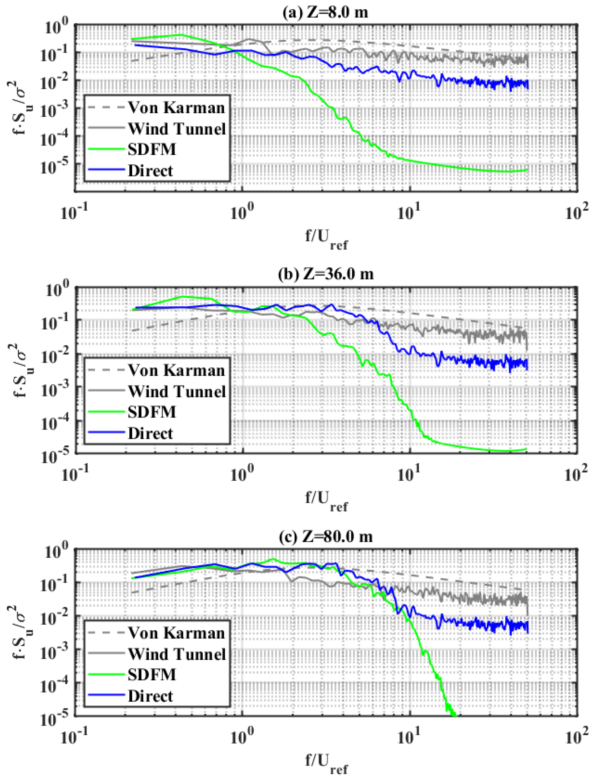
Focusing on the results of Figure 8, the SDFM seems to provide valid spectral content for fluctuations until 70 Hz ($U_{ref}$ = 9.26 m/s), for all heights examined. The direct method is closer to the experimental results, and more accurate as the height is increased, although some deviation can be spotted at 8 m for the high part of the frequency. The spectral content in these heights seems to agree with experimental results since the time series measured in the computational domain are strongly related to the wind tunnel data that are directly applied in the inlet plane. Moving to the point of interest, C, in Figure 9, the SDFM seems to agree with the experimental spectrum until 70 Hz for 80 m, 15 Hz for 36 m, and 10 Hz for 8 m ($U_{ref}$ = 9.92 m/s). The direct method follows a similar trend as seen in point PO of Figure 8, but underestimates the spectrum at the high part of the frequency domain in all heights, due to the filter of the subgrid model, which affects the high frequencies. Furthermore, at 8 m, the direct method seems to slightly underestimate the spectral content in the entire range of the frequency domain.

The significant deviations from the target values in both locations, especially in the high part of the frequency domain, agree with references [14,17,22,28] and lead to two remarks. First, synthetic methods are unable to establish a valid spectral content for the low part of the ABL, where the low-rise buildings reside, as seen in Figure 9a,b. Second, in larger heights of the ABL (80 m), where most results can be found in the literature, the spectral content underestimates the high part of the frequency domain for both methods. These high-frequency velocity fluctuations are related to the high-frequency pressure fluctuations in the building envelope, which play a fundamental role in the calculation of peak (design) values. As a next step, it is important to tune the virtual and the physical wind tunnel, to represent the same content for these high fluctuations.

4. Dynamic Terrain Method

To tune the spectral content between computational and experimental procedures, the concept of the dynamic terrain was introduced. The target is to establish a technique that optimizes the frequency in which velocities are inserted into the computational domain, to introduce more high-frequency fluctuations in the location of interest, without inflating the mesh and decreasing the filter size. In order to navigate through the complexity of inlet conditions, the proposed method was given this name to emphasize the dynamic nature of the transition of the turbulence features in the computational domain, from the inlet plane until the location of interest. The accurate spectral representation in the location of interest is the goal of the method, and as a second step, the rest of the turbulence statistics can be re-calibrated individually.

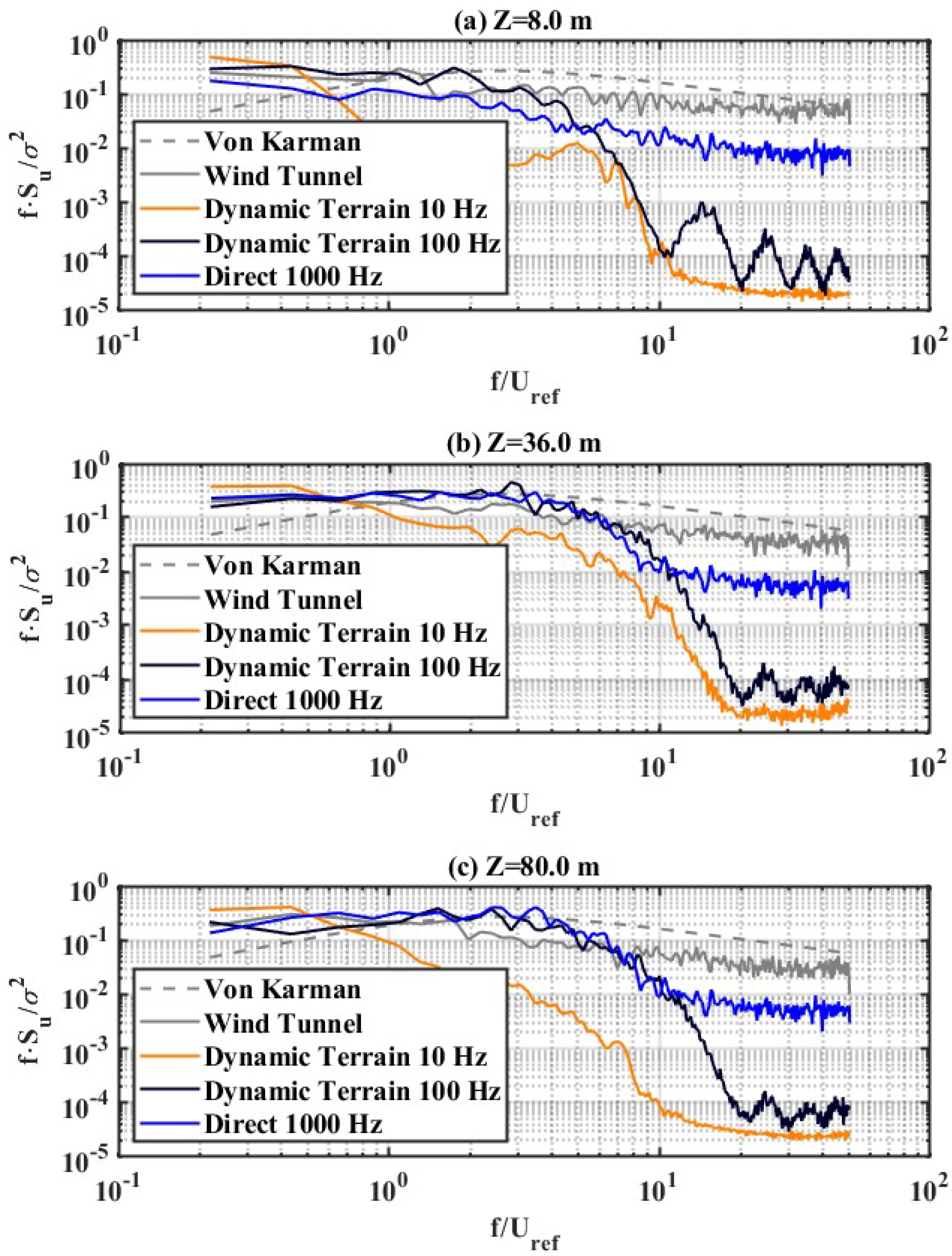
The procedure of the method is similar to the direct one since the extracted time series from the wind tunnel measurements are introduced in the computational domain, but with the very important difference that the input frequencies of the data are adapted. In the first part of the parametric study, the imposed frequency of the velocity was selected as smaller than the one found in the direct method (1000 Hz), and the target comparisons regard the turbulence intensity and the spectral content in locations PO and C. For dynamic terrain 10 Hz (DT10), every 100th value was stored, and a new time series was constructed with a uniform time step of 0.1 s and introduced in the computational domain. For dynamic terrain 100 Hz (DT100), every 10th value was stored, and the new time series was introduced in the inlet boundary with a time step of 0.01s. The corresponding mean speed, turbulence intensity, and turbulence length scale distributions with height are identical to the extracted results of 1000 Hz from the wind tunnel probe.

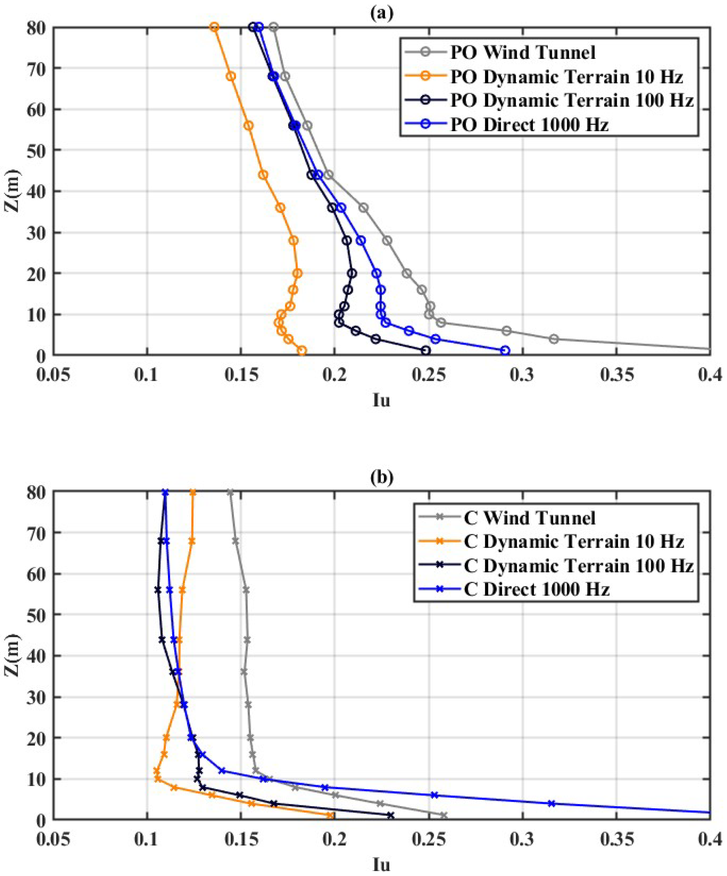
In Figure 10, the turbulence intensity at points PO and C is presented for the dynamic terrain methods and the direct one. At PO, a proportional relationship can be seen between the imposed frequency and the calculated turbulence intensity; the higher frequencies provide results closer to the experimental target. At point C, this linear pattern can be spotted for the first 10 m of the layer, and after that, the direct method agrees with the DT100. Above 40 m, the DT10 values are closer to the experimental results, while in both locations, the direct and DT100 results agree. The deviations under 40 m can be considered acceptable, especially when reviewing the corresponding deviations found in the literature and database sets from wind tunnel experiments in similar terrains. Point C was selected for the spectral representation of the methods for the same heights as in Section 3, as seen in Figure 11. DT10 underpredicts the spectral content in all heights, while DT100 agrees with the spectrum until70 Hz, exactly as the SDFM in Section 3. A main difference with the SDFM is that DT100 can present the fluctuations in the lower part (Figure 9a and Figure 11a) until 30 Hz.

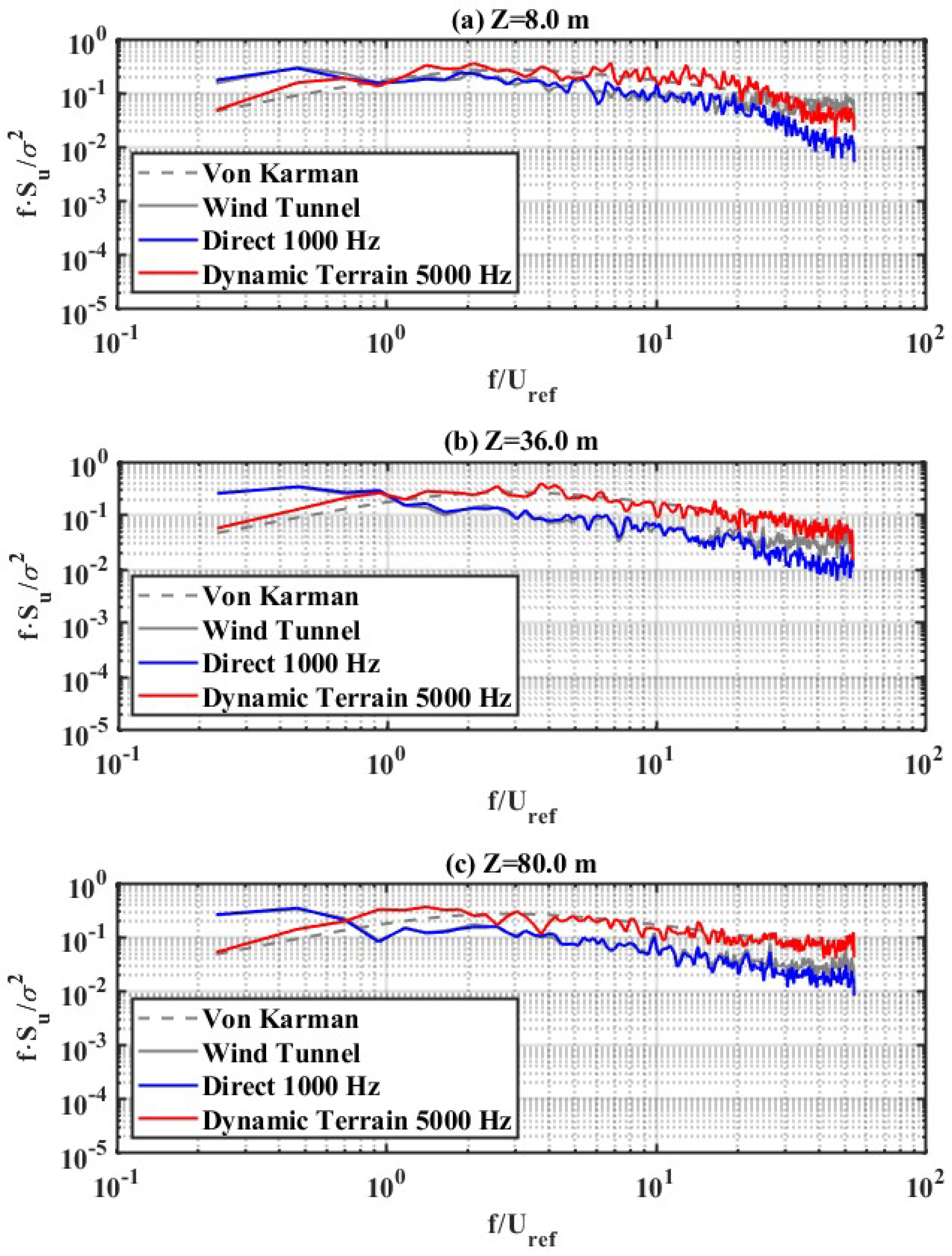
Figure 11 shows the proportional relationship of the spectral content in the high part of the domain and the imposed frequency of the inlet velocity at the boundary. The inlet frequency seems to correlate with the ability of LES to represent the actual spectral content measured from experiments, which is why in the second leg of the study, this frequency was increased higher than the experimental output of 1000 Hz. Dynamic terrain 5000 Hz (DT5000) uses the time series from all five segments of the extracted results, and a uniform time step of 0.0002 s was employed. Every velocity measurement was stored, and new time series were constructed with a total duration of 6.6 s. This total duration is the same as the ones used for all the methods of the study, and it is important to mention that the statistical characteristics are the same at the inlet boundary. Larger time series were also tested as inlet conditions, and the variation in the results was proven to be negligible.

In Figure 12, the turbulence intensity distribution of DT5000 is compared with the experiments and the direct method for PO and C. Results at PO indicate a small underestimation of the intensity under 40 m. Above this limit, good accuracy is achieved, since the inlet values are closely related to the experimental data close to the inlet plane. At location C, DT5000 and the direct method provide the same values for the first 10 m of the boundary layer, with small deviations above this height. In the last few years, various assumptions have been used to correct the turbulence decay in the computational domain from PO to location C. While using the random flow generator method, Guichard [29] augmented the inlet intensity by calculating an “adapted” distribution, which considers the turbulence decay calculated in the domain in an initial analysis. While using the digital filter method, which is used in Section 3 of this paper, Lamberti et al. [17] optimized the input values to deal with the decay. In both approaches, the fact that the turbulence intensity is valid in the building location does not guarantee that the spatial coherency of the turbulent structures is expressed correctly; thus, special attention is needed for the practical use of synthetic methods, with more comparisons of the turbulent features in various locations of the domain.

In this respect, in the DT5000 method, although it does not represent accurately the turbulence decay, an augmentation of the inlet intensity is feasible, but not in line with the targets of the current work. At this point, the main target is to generate high-frequency fluctuations without having to decrease the filter size, which leads to non-manageable computational domains for practitioners. An initial parametric study has proven that there is no correlation between the ability of the method to capture the high part of the frequency domain and the modification at the inlet turbulence intensity to take care of the turbulence decay; thus, this can be addressed as a next step. For the time being, the drawback of this method is obvious, since capturing the turbulence intensity in the ABL profile is vital for a proper design. It is important to mention that the turbulence intensity at the target roof height of 8 m for the building at location C is in good agreement with the experimental data; thus, according to Tieleman [27], the fluctuating pressure values on the building envelope should be well related to the full-scale data.

In Figure 13, the spectral content is displayed at location PO, where DT5000 provides values closer to the experimental and theoretical results than the direct approach. In all heights, DT5000 seems to agree better with the theoretical von Karman spectrum than the experimental results.

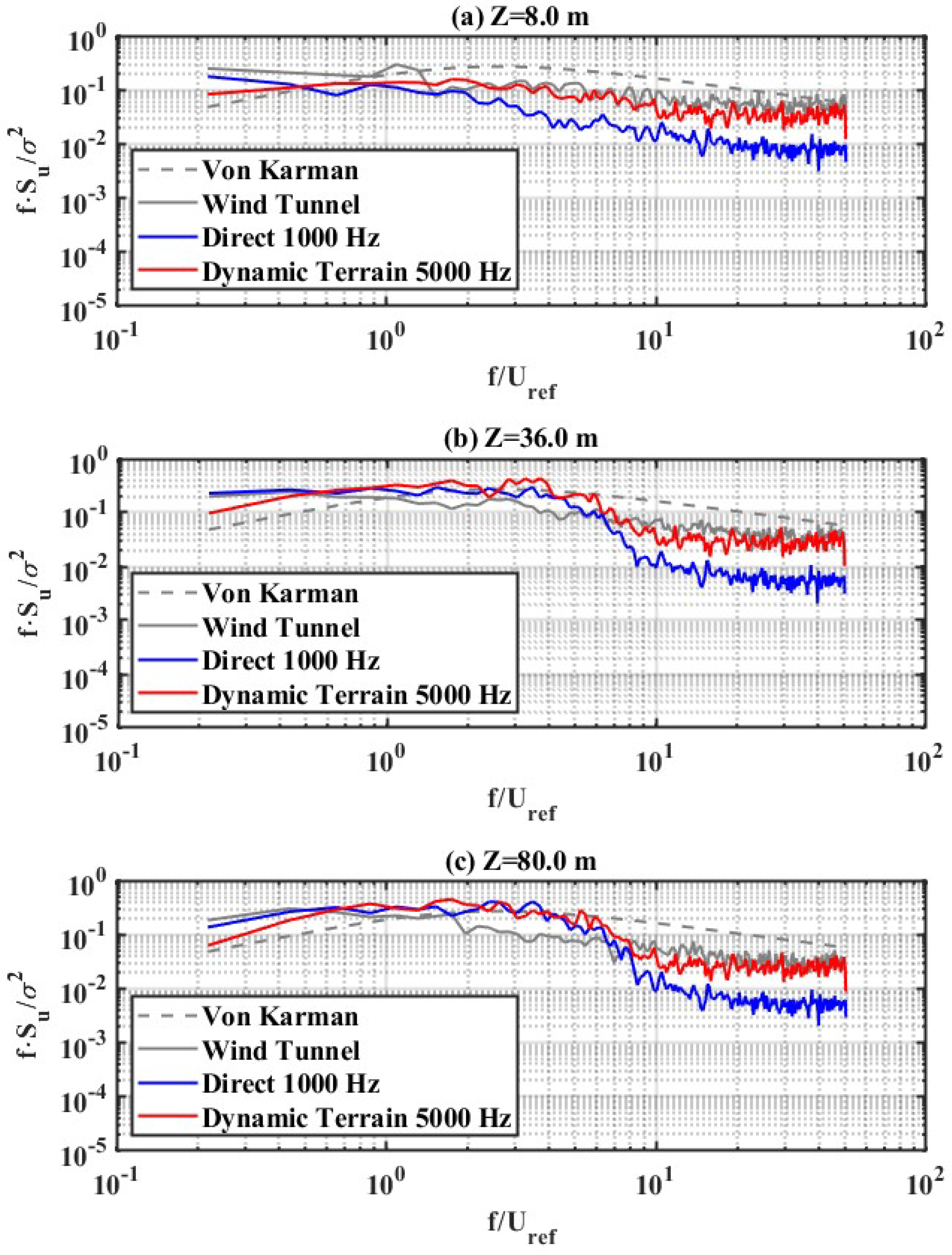
Finally, in Figure 14 the superiority of the DT5000 method is evident for the location of interest, C. At all heights examined, the spectral content of the method is compatible with the experimental results, especially for the high part of the frequency domain. These results contradict the notations in Melaku et al. [14] and Thomas et al. [46], which mention that the misrepresentation of the high part of the frequency domain is unavoidable and related to the inaccuracy in the solution of the subgrid model of LES. “This issue has been noticed in LES and is due to the numerical dissipation in the finite difference scheme (Thomas and Williams, 1999)”. On the other side, it proves that the inlet conditions are a more sensitive component in the spectral domain representation than the mesh size and the corresponding application due to the subgrid model. The expression of these high-frequency fluctuations, related to small-scale turbulence structures, while the mesh size is constant, indicates the merit of the method for the construction of an ABL in LES that respects turbulent features and their spatial coherency.

5. Summary and Conclusions

The present paper worked towards innovating the current state-of-the-art regarding the expression of the turbulent structure of the incoming wind load in LES applications. Experiments from the Concordia University Building Aerodynamics Laboratory were compared with a Virtual Wind Tunnel in the OpenFOAM open software. Focus was given to the high-frequency fluctuations on the lower part of the atmospheric boundary layer for efficient low-rise building design. Results proved the ability of the proposed method to simulate these high-frequency, small-scale fluctuations in the calculated spectrum, with simple assumptions that regard the dynamic nature of the inlet velocity profile.

Experiments proved that turbulence decay is superior in the first 40 m of the atmospheric boundary layer; thus, special attention needs to be sought for low-rise building applications. The characteristic intensity in the building height plays a key role in the correct estimation of surface pressures in low-rise buildings, so the turbulence decay must be taken properly into account when calculating the design loads to match full-scale conditions in LES. Numerical results from all models of the article suggest that turbulence features decay closer to the inlet boundary when compared with the experimental values, when not using augmentation techniques for the inlet intensity.

In the first leg of the study, synthetic methods were used as the inlet conditions for the velocity to estimate the accuracy of two fundamental aspects: the turbulence evolution in the streamwise direction via second-order normalized statistics (intensity and integral length scale) and the spectral content. In the SDFM technique, the spectral content in the heights of interest for low-rise buildings deviates extremely from theoretical and experimental results. The first leg of the study also regards the direct method, where the inlet velocity imposed in the virtual boundary matches the one from the experimental measurements. Direct method results were compared with the synthetic inlet and proved that turbulent decay features for the turbulent intensity, integral length scale, and spectral content are superior for the former in the lower part of the ABL.

The second leg of the parametric study consisted of the implementation of the so-called dynamic terrain method. This method does not belong to the synthetic or cyclic methods, but it uses velocity time histories from experimental measurements as direct inlet conditions in the virtual wind tunnel computational domain. The imposed frequency at the virtual inlet boundary consists of the only difference between the various models. Results indicate that a proportional relationship exists between the capacity of the mesh to capture the correct energy content of the fluctuations with the imposed frequency at the inlet boundary. The parametric study proved that higher imposed frequencies increase the abilities of the mesh to represent the high part of the frequency domain and that inlet conditions are a more sensitive parameter for the spectrum representation than the numerical schemes, the mesh size, and the subgrid model. The results of the method in the lower part of the ABL match the theoretical and experimental results, making it ideal for low-rise building design. A clear advantage of such an application refers to less expensive computational tools and simple procedures, easily understood and applied by practitioners. Future targets of this work regard validation of the method for the pressure contour when a low-rise building is placed in location C.