Abstract
The effect of the sky view factor (SVF) on outdoor thermal comfort has been extensively explored, while its impact on the indoor thermal environment is ignored. This research combined Envi-met and kriging models to explore the annual effect of the sky view factor on the indoor thermal environment. Different from previous studies, this study explored the effect of the sky view factor on indoor temperature rather than outdoor temperature, and from the perspective of a full year instead of a typical summer day. The analytical results reveal that an increase in the sky view factor raised the indoor air temperature every month. Although a low sky view factor was beneficial to the insulation of the built environment at night, it was proven that in Chenzhou city, the indoor air temperature was still higher in a built area with a high sky view factor than with a low sky view factor. In addition, the sky view factor was shown to have a nonlinear relationship with indoor thermal comfort throughout the year. When the sky view factor increased from 0.05 to 0.45, the indoor temperature increased by around 10 °C at 16:00 and increased by about 4 °C throughout the night for each month, and from the view of the annual cycle, the cooling demand duration increased by 1611.6 h (18.4%), and the heating demand duration decreased by 1192.3 h (13.61%).
1. Introduction
High-density cities save land; however, they inevitably compromise the quality of the urban environment, such as by blocking ventilation, enhancing the urban heat island (UHI) effect, and aggravating pollution [1,2,3]. Especially in high-density urban areas, the sky view is narrowed by surrounding buildings [4,5]. The diminished visual range and thermal environment this causes are areas of concern being examined by urban planning scholars [6,7]. Oka initially pointed out that UHI depends on the size and meteorology of the city [8]. The sky view factor (SVF) is an important index for urban planners to describe urban morphology and is defined as the ratio of the amount of sky visible from a given point on a surface to the potentially available amount [9,10]. SVF is a dimensionless number ranging from 0 to1 [11]. Usually, the SVF at any point in a city is less than 1, because the surrounding buildings cover the visible sky. In principle, a high SVF during the day means more shortwave radiation entering street canyons, increasing the ambient air temperature [12,13]. At night, a low SVF blocks the divergence of longwave radiation in street canyons, which in turn blocks heat dissipation and raises the air temperature [14,15]. Existing studies have confirmed that SVF has strong relationships with land surface and wall surface temperature [16,17,18,19]. Because shortwave radiation is the main contributor to urban surface and building wall surface temperature, it is consequently strongly affected by SVF. In terms of air temperature, most studies, including Eliasson’s investigation in Goteborg, Sweden [20], and Taha’s investigation in San Francisco, USA, point out that the sensitivity of air temperature to SVF variation is weak [21]. However, Svensson observed a strong relationship between SVF and night-time air temperature in Goteborg using mobile observation and weather station data [22]. Recently, Ha reported that SVF negatively affected air temperature in Seoul, Korea, both during the day and at night [23]. The conclusions regarding the effect of SVF on outdoor air temperature in different experiments differ, and some even contradict each other. This is because, compared with land surface and wall surface temperature, outdoor air temperature is affected by multiple factors such as radiation, convection, and heat conduction [24,25]. Therefore, the correlation between air temperature and SVF is not as strong as that between SVF and surface temperature.
Existing studies have explored the impact of SVF on outdoor surface and air temperature [26,27,28,29], and some studies have further explored its impact on outdoor thermal comfort [30,31,32]. Different from outdoor air temperature, the indoor air temperature of a closed room is, in principle, determined by the wall temperature and the radiation transmitted through the transparent glass of windows [33,34,35], which is strongly affected by SVF. However, thus far, there is no research exploring how SVF affects indoor air temperature. The reason for this research gap is that urban planning scholars concentrate on the outdoor environment, and architectural scholars are more concerned about the indoor environment, but they all ignore the impact of outdoor morphology on the indoor environment. Improving the indoor thermal environment could reduce the energy consumption of buildings, because the indoor air temperature needs to be conditioned for thermal comfort [36], which is different from the outdoor thermal environment. In hot summer and cold winter climate zones, cooling the indoor temperature is beneficial to the indoor thermal environment in summer, but it is harmful in winter [37,38] in terms of indoor thermal comfort. Therefore, we cannot copy the method of evaluating the impact of SVF on the indoor thermal environment on a typical summer day. In this study, instead, annual cycle evaluation based on the kriging model, a temperature interpolation method, is proposed to evaluate the impact of SVF on the indoor thermal environment.
2. Methods and Parameters
2.1. Analytical Scenarios
Chenzhou, a city with cold winters and hot summers located in the south of Hunan, China, was selected as the research city [39]. We calculated the SVF of the main streets in Chenzhou with digital data. The SVF values of the main streets in Chenzhou are shown in Figure 1, which illustrates that the values ranged from 0.1 to 1.
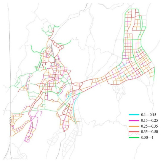
Figure 1.
SVF values of main streets in Chenzhou city.
In China, the width of both urban and residential roads follows unified national standards. Urban trunk roads are 30–40 m wide, secondary trunk roads are 20–24 m wide, and branch roads are 14–18 m wide. The width of roads connecting residential groups is 10–14 m, and the width of roads in residential groups is 5–7 m. Therefore, the SVF within Chenzhou residential areas is calculated to be 0.075–0.25. For residential buildings facing urban streets, the SVF can still reach 0.5. As Envi-met model is composed of grids, it cannot construct any SVF value model. Therefore, we selected 0.05, a value close to 0.075 as the lower bound, and 0.45, a value close to 0.5 as the upper bound. Based on the above analysis, we adopted 0.05, 0.18, 0.3, 0.4, and 0.45 as the representative SVF values of residential areas in Chenzhou. The five models corresponding to these five SVF values are shown in Figure 2.
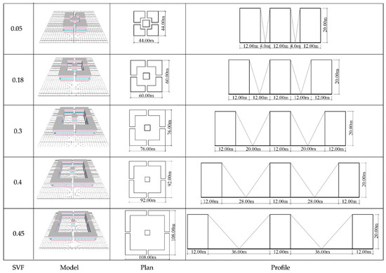
Figure 2.
Models with different SVF values.
In Figure 2, the scale and shape of the 5 buildings in the center of the building groups are the same, with a ground floor area of 12 × 12 m2 and height of 20 m. The window-to-wall ratios of the buildings are 20%. The buildings walls have a thickness of 300 mm, and are composed of hollow concrete brick, with a roughness length of 0.02. The attributes of hollow concrete brick are presented in Table 1 [40]. In addition, the roof is made of reinforced concrete, whose parameters are shown in Table 2 [41].

Table 1.
Attributes of hollow concrete brick.
Table 2.
Attributes of reinforced concrete.
In Chenzhou, clear float glass is commonly used in residential buildings; thus, we used clear float glass as the windows in the simulation. The parameters of clear float glass are presented in Table 3 [42].
Table 3.
Attributes of clear float glass.
2.2. Simulation Tools
We employed the Envi-met model to explore the effect of SVF on the indoor thermal environment. Envi-met is designed to simulate the interactions between surface–plant–air in the city, and it has 10 programs and 10 functions (https://www.envi-met.com/software/; accessed on 1 May 2022). Although many simulation tools can calculate indoor air temperature, such as Ecotect [43], TRNSYS [44], and EnergyPlus [45], these models are not CFD-based programs. In these programs, the wind speed is fixed in only one direction, which cannot accurately describe the effects of wind on convective heat transfer on facades [46]. Envi-met is a non-hydrostatic, micro-climatological, and computational fluid dynamics model that incorporates thermodynamic principles [47]. Envi-met simulates indoor air temperature by calculating the heat convection on the associated interior walls and roofs, as well as the energy transmitted through the transparent glass. The indoor temperature follows Equation (1) [48]:
where indicates the initial air temperature in zone i, V is the volume of zone i, and is the updated air temperature in zone i after time dt; A(e) is the surface area of zone i, and E is the number of façades in zone i; is the shortwave radiation transmitted into zone i through transparent glass e; and is the heat convection coefficient of the sensible heat transfer between the indoor air and interior walls.
Many published studies have tested the accuracy of the Envi-met model by field experiments [49,50]. Previous studies have revealed that, for Envi-met, the correlation coefficient between simulated indoor air temperatures and measured indoor air temperatures is 0.956 in a greening wall experiment [40]. We also carried out an experiment to validate the accuracy of the Envi-met model in simulating the indoor air temperature, the details of which are shown in the published paper, where the R2 of simulated and measured temperature was 0.902 [42], which validated the accuracy of the Envi-met model in the indoor air temperature simulation.
2.3. Meteorological Data and Settings
The meteorological data of Chenzhou city from 2007 to 2020 were collected from the website of historical weather (https://tianqi.2345.com/wea_history/57972.htm; accessed on 11 April 2021). Based on the historical data, we calculated mean air temperature, average wind speed, and relative humidity (RH) for every month. These data were employed as the boundary conditions for evaluating the annual effects of SVF on the indoor thermal environment in Chenzhou. The specific monthly boundary conditions are shown in Table 4.
Table 4.
Boundary conditions of simulation.
3. Results and Discussion
3.1. Effects of SVF on Indoor Thermal Environment for Each Month
The Envi-met model was used to simulate the indoor air temperature in five SVF models, and 1440 indoor air temperatures were obtained (5 SVF models × 24 h in a day × 12 months in a year). To visually display the simulation results, Figure 3 shows the simulated results at 16:00 in January, when indoor temperatures were collected from the center building.
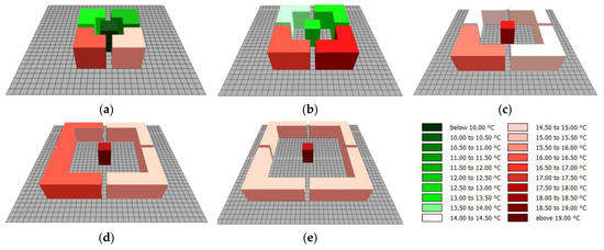
Figure 3.
Simulation results at 16:00 in January. (a) Indoor air temperature at 16:00 in January for the SVF (0.05) scenario. (b) Indoor air temperature at 16:00 in January for the SVF (0.18) scenario. (c) Indoor air temperature at 16:00 in January for the SVF (0.3) scenario. (d) Indoor air temperature at 16:00 in January for the SVF (0.4) scenario. (e) Indoor air temperature at 16:00 in January for the SVF (0.45) scenario.
To further understand the daily variations of indoor air temperature, we conducted a statistical analysis of indoor temperature changes under the five SVF scenarios in every month, the results of which are presented in Figure 4.
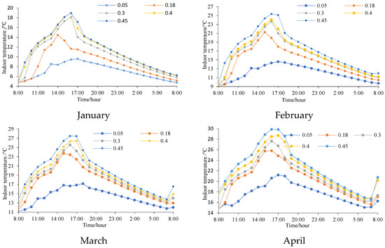
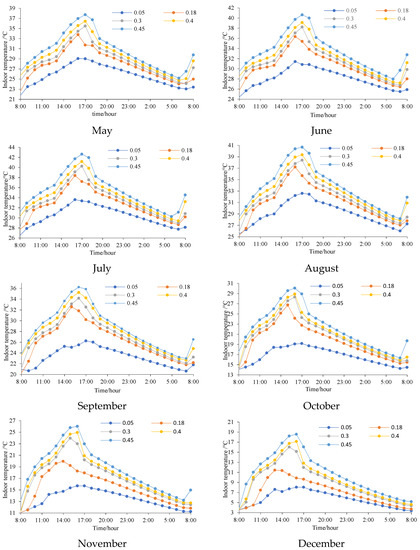
Figure 4.
Daily variations of indoor temperature under 5 SVF conditions over 12 months.
Figure 4 shows that in Chenzhou city, high SVF improved daily indoor air temperatures in every month. When the SVF increases from 0.05 to 0.45, the indoor temperature increases by around 10 °C at 16:00 for each month when SVF causes the maximum temperature difference on the indoor thermal environment. This phenomenon is easy to understand in the daytime, when solar radiation is the main contributor to increased indoor air temperature. Residential blocks with high SVF allow buildings more access to solar radiation, which raises the indoor air temperature.
Different from the daytime, the influence mechanism of indoor temperature at night is more complex. Without solar radiation, buildings continue to dissipate heat, and accordingly, the indoor temperature gradually decreases. Existing studies have proven that at night, areas with low SVF block the dissipation of longwave radiation by multiple reflection in urban canyons, forming urban heat islands; in particular, streets with high SVF values are conducive to building heat dissipation. Conversely, compared with buildings in blocks with low SVF, buildings in blocks with high SVF also accumulate more heat during the day, forming higher indoor temperatures. Therefore, at night, there may be two cases of indoor temperatures of residential areas with different SVF values. First, indoor temperatures in residential areas with high SVF are always higher than those in areas with low SVF throughout the night. Second, indoor temperatures of residential areas with high SVF decrease faster and are lower compared to residential areas with high SVF from a certain time of the night. One of these two scenarios will occur, depending on the local climate and building materials. Figure 3 illustrates that high SVF keeps the indoor temperature higher than low SVF throughout the night in Chenzhou city. Furthermore, when the SVF increased from 0.05 to 0.45, the mean indoor temperature during the night increased by about 4 °C for each month.
3.2. Effects of SVF on Indoor Thermal Environment for Each Month
While the daily variation in indoor temperature every month can be used to explore the effects of SVF, it cannot determine the advantages and disadvantages of different SVF values on the indoor thermal environment over a full year. To explore the annual effects of SVF on the indoor thermal environment in Chenzhou city, the kriging model was used to fit the annual distribution of indoor air temperature under the five SVF scenarios. Kriging is a feasible model to use for interpolating temperature values [51]. The kriging model’s built-in Surfer software was employed as the translation tool in this research. With the help of the kriging model, we determined the annual distribution of indoor air temperature for the five SVF scenarios (SVF = 0.05, 0.18, 0.30, 0.40, and 0.45), as shown in Figure 5.
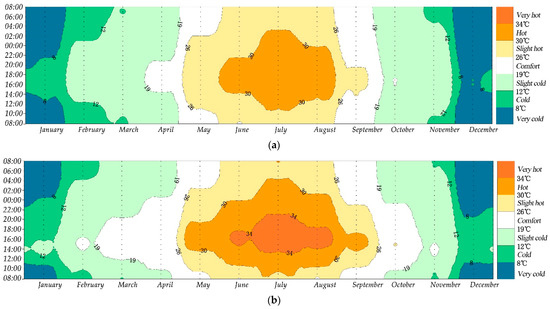
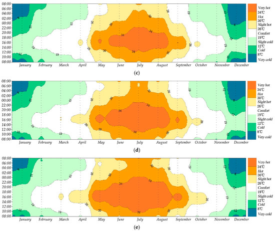
Figure 5.
Distribution of annual indoor air temperature for 5 SVF scenarios. (a) Annual distribution of indoor air temperature for the five SVF (0.05). (b) Annual distribution of indoor air temperature for the five SVF (0.18). (c) Annual distribution of indoor air temperature for the five SVF (0.30). (d) Annual distribution of indoor air temperature for the five SVF (0.40). (e) Annual distribution of indoor air temperature for the five SVF (0.45).
Figure 5 indicates that with increased SVF values, the perception of “very cold” decreased substantially, and the perception of “very hot” increased markedly on an annual basis. Compared with the scenario of SVF = 0.05, under the other four scenarios, the duration of “comfort” was extended by a similar proportion.
To accurately quantify the annual impact of SVF on the indoor thermal environment, the duration and proportion of thermal perception under the five SVF scenarios were statistically analyzed. By calculating the area of the proportion of thermal perception on the map, we converted it into duration. The duration and proportion of thermal perception on an annual basis are presented in Table 5.
Table 5.
Proportion and duration of indoor thermal perception for 5 SVF scenarios.
Table 5 shows that, in general, high SVF markedly reduced the thermal perception of “very cold”, “cold”, and “slightly hot”, but extended the duration of “hot” and “very hot”. To evaluate the general impact of SVF on indoor thermal comfort on an annual basis, perceptions of “comfortable”, “slightly cold”, and “slightly hot” were regarded as acceptable. In addition, “cold”, “very cold”, “hot”, and “very hot” were treated as unacceptable, as they require the use of energy to improve the indoor temperature. For SVF values of 0.05, 0.18, 0.30, 0.40, and 0.45, the corresponding proportions of acceptable thermal perception were 5698.9 h (65.1%), 5503.5 h (62.8%), 5653.3 h (64.5%), 5437.0 h (62.1%), and 5279.5 h (60.3%). Accordingly, the proportions of unacceptable thermal perception were 3061.1 h (34.9%), 3256.5 h (37.2%), 3106.7 h (35.5%), 3322.9 h (37.9%), and 3480.1 h (39.7%). The variations in acceptable and unacceptable thermal perception indicated that SVF had a nonlinear relationship with indoor thermal comfort throughout the year in Chenzhou city. Further, this research also took “very cold” and “cold” as the heating demand duration of the building and “very hot” and “hot” as the cooling demand duration. Thus, the duration of heating demand for the building under the five SVF scenarios was 2058.75 h (23.50%), 1585.1 h (18.09%), 1120.9 h (12.80%), 1010.6 h (11.54%), and 866.5 h (9.89%), and for cooling demand, the duration was 1002.3 h (11.44%), 1671.4 h (19.08%), 1985.7 h (22.67%), 2312.3 h (26.40%), and 2613.9 h (29.84%). Statistical data revealed that when the SVF increased from 0.05 to 0.45, the heating demand duration decreased by 1192.3 h (13.61%) and the cooling demand duration increased by 1611.6 h (18.4%).
4. Conclusions
Many studies have explored the impacts of SVF on air temperature, mean radiation temperature, surface temperature and thermal comfort [32]. Compared with radiation temperature, surface temperature and thermal comfort, the impact of SVF on outdoor air temperature is not appreciable, which is caused by other factors such as land use [32]. For example, a park near the street may affect the ambient temperature when analyzing the effects of SVF on outdoor air temperature. However, for an indoor thermal environment, the effect of SVF is appreciable. The analytical data revealed that an increase in SVF increased the indoor air temperature in every month of the year. When the SVF rose from 0.05 to 0.45, the indoor temperature increased by around 10 °C at 16:00 for each month. Although low SVF was beneficial to the insulation of the built environment at night, it was proven that in Chenzhou city, high SVF still kept the indoor temperature higher than low SVF throughout the night in every month because it allows more heat to accumulate during the daytime. In Chenzhou, when the SVF increased from 0.05 to 0.45, the mean indoor temperature during the night increased by about 4 °C for each month.
In addition, by applying the kriging model, we further explored the effects of SVF on thermal distribution on an annual basis. The analytical data indicated a nonlinear relationship between SVF and indoor thermal comfort throughout the year in Chenzhou city. The durations of heating demand for buildings with SVF values of 0.05, 0.18, 0.30, 0.40, and 0.45 were 2058.75 h (23.50%), 1585.1 h (18.09%), 1120.9 h (12.80%), 1010.6 h (11.54%), and 866.5 h (9.89%), respectively, and the durations of cooling demand were 1002.3 h (11.44%), 1671.4 h (19.08%), 1985.7 h (22.67%), 2312.3 h (26.40%), and 2613.9 h (29.84%), respectively.
When SVF increased from 0.05 to 0.45, heating demand duration decreased by 1192.3 h (13.61%) and cooling demand duration increased by 1611.6 h (18.4%). With an increase in SVF, the increased cooling demand duration was longer than the reduced heating demand duration, which means that the acceptable thermal perception throughout the year was reduced by 419.3 h (4.79%) when SVF increased from 0.05 to 0.45. Therefore, increasing SVF in residential areas is unfavorable to the indoor thermal environment in Chenzhou all year round. Different from advocating increasing SVF to reduce the urban heat island effect [22], this study points out that in the hot summer and cold winter climate zone, high SVF may be beneficial to the outdoor thermal comfort in summer, but it is unfavorable to the indoor thermal comfort from the view of the annual cycle.
Different from the influence of SVF on outdoor thermal comfort on typical summer weather days, this study analyzed the influence of SVF on the indoor thermal environment from the perspective of the annual cycle, which provided us with a deeper understanding of SVF. Meanwhile, there are still some limitations in the study that need to be explored further.
(1) This research evaluated the impact of SVF on indoor thermal comfort but did not evaluate the corresponding energy consumption demand of cooling or heating.
(2) The SVF values of streets around buildings are not always uniform in real cities. It would be useful to determine the results of different SVF combinations.
Author Contributions
Conceptualization, J.L. and B.Z.; methodology, J.L.; software, J.L.; validation, J.L.; formal analysis, B.Z.; investigation, J.L.; resources, J.L.; data curation, B.Z.; writing—original draft preparation, J.L.; writing—review and editing, J.L.; visualization, J.L.; supervision, B.Z.; project administration, J.L.; funding acquisition, B.Z. All authors have read and agreed to the published version of the manuscript.
Funding
This research was funded by the China Scholarship Council, grant number 202006370126, and the Hunan Provincial Philosophy and Social Science Planning Fund Office, grant number XSP20ZDI020.
Institutional Review Board Statement
Not applicable.
Informed Consent Statement
Not applicable.
Data Availability Statement
The data are available on request from the corresponding author.
Acknowledgments
Thanks are given to the National University of Singapore for help in the field experiment.
Conflicts of Interest
The authors declare no conflict of interest.
References
- Lan, H.; Lau, K.K.-L.; Shi, Y.; Ren, C. Improved urban heat island mitigation using bioclimatic redevelopment along an urban waterfront at Victoria Dockside, Hong Kong. Sustain. Cities Soc. 2021, 74, 103172. [Google Scholar] [CrossRef]
- Adelia, A.; Yuan, C.; Liu, L.; Shan, R. Effects of urban morphology on anthropogenic heat dispersion in tropical high-density residential areas. Energy Build. 2019, 186, 368–383. [Google Scholar] [CrossRef]
- Li, J.; Zheng, B.; Ouyang, X.; Chen, X.; Bedra, K.B. Does shrub benefit the thermal comfort at pedestrian height in Singapore? Sustain. Cities Soc. 2021, 75, 103333. [Google Scholar] [CrossRef]
- Mirzaee, S.; Özgun, O.; Ruth, M.; Binita, K. Neighborhood-scale sky view factor variations with building density and height: A simulation approach and case study of Boston. Urban Clim. 2018, 26, 95–108. [Google Scholar] [CrossRef]
- Guo, J.; Han, G.; Xie, Y.; Cai, Z.; Zhao, Y. Exploring the relationships between urban spatial form factors and land surface temperature in mountainous area: A case study in Chongqing city, China. Sustain. Cities Soc. 2020, 61, 102286. [Google Scholar] [CrossRef]
- Zhou, H.; Tao, G.; Nie, Y.; Yan, X.; Sun, J. Outdoor thermal environment on road and its influencing factors in hot, humid weather: A case study in Xuzhou City, China. Build. Environ. 2022, 207, 108460. [Google Scholar] [CrossRef]
- Chen, T.; Pan, H.; Lu, M.; Hang, J.; Lam, C.K.C.; Yuan, C.; Pearlmutter, D. Effects of tree plantings and aspect ratios on pedestrian visual and thermal comfort using scaled outdoor experiments. Sci. Total Environ. 2021, 801, 149527. [Google Scholar] [CrossRef]
- Oke, T.R. Boundary Layer Climates; Routledge: Abingdon-on-Thames, UK, 2002. [Google Scholar]
- Yuan, C.; Chen, L. Mitigating urban heat island effects in high-density cities based on sky view factor and urban morphological understanding: A study of Hong Kong. Archit. Sci. Rev. 2011, 54, 305–315. [Google Scholar] [CrossRef]
- Bernard, J.; Bocher, E.; Petit, G.; Palominos, S. Sky view factor calculation in urban context: Computational performance and accuracy analysis of two open and free GIS tools. Climate 2018, 6, 60. [Google Scholar] [CrossRef] [Green Version]
- Yin, C.; Yuan, M.; Lu, Y.; Huang, Y.; Liu, Y. Effects of urban form on the urban heat island effect based on spatial regression model. Sci. Total Environ. 2018, 634, 696–704. [Google Scholar] [CrossRef]
- Kim, E.-S.; Yun, S.-H.; Park, C.-Y.; Heo, H.-K.; Lee, D.-K. Estimation of mean radiant temperature in urban canyons using Google Street View: A case study on Seoul. Remote Sens. 2022, 14, 260. [Google Scholar] [CrossRef]
- Boccalatte, A.; Fossa, M.; Gaillard, L.; Menezo, C. Microclimate and urban morphology effects on building energy demand in different European cities. Energy Build. 2020, 224, 110129. [Google Scholar] [CrossRef]
- Yu, Z.; Chen, S.; Wong, N.H.; Ignatius, M.; Deng, J.; He, Y.; Hii, D.J.C. Dependence between urban morphology and outdoor air temperature: A tropical campus study using random forests algorithm. Sustain. Cities Soc. 2020, 61, 102200. [Google Scholar] [CrossRef]
- Dirksen, M.; Ronda, R.; Theeuwes, N.; Pagani, G. Sky view factor calculations and its application in urban heat island studies. Urban Clim. 2019, 30, 100498. [Google Scholar] [CrossRef]
- Scarano, M.; Mancini, F. Assessing the relationship between sky view factor and land surface temperature to the spatial resolution. Int. J. Remote Sens. 2017, 38, 6910–6929. [Google Scholar] [CrossRef]
- Guo, G.; Zhou, X.; Wu, Z.; Xiao, R.; Chen, Y. Characterizing the impact of urban morphology heterogeneity on land surface temperature in Guangzhou, China. Environ. Model. Softw. 2016, 84, 427–439. [Google Scholar] [CrossRef]
- Yang, J.; Shi, Q.; Menenti, M.; Wong, M.S.; Wu, Z.; Zhao, Q.; Abbas, S.; Xu, Y. Observing the impact of urban morphology and building geometry on thermal environment by high spatial resolution thermal images. Urban Clim. 2021, 39, 100937. [Google Scholar] [CrossRef]
- Zhang, Y.; Middel, A.; Turner, B. Evaluating the effect of 3D urban form on neighborhood land surface temperature using Google Street View and geographically weighted regression. Landsc. Ecol. 2019, 34, 681–697. [Google Scholar] [CrossRef]
- Eliasson, I. Urban nocturnal temperatures, street geometry and land use. Atmos. Environ. 1996, 30, 379–392. [Google Scholar] [CrossRef]
- Taha, H. Night Time Air Temperature and The Sky-View Factor: A Case Study in San Francisco, California; Lawrence Berkeley Laboratory: Berkeley, CA, USA, 1988. [Google Scholar]
- Svensson, M.K. Sky view factor analysis–implications for urban air temperature differences. Meteorol. Appl. 2004, 11, 201–211. [Google Scholar] [CrossRef]
- Ha, J.; Lee, S.; Park, C. Temporal effects of environmental characteristics on urban air temperature: The influence of the sky view factor. Sustainability 2016, 8, 895. [Google Scholar] [CrossRef] [Green Version]
- Lin, T.-P.; Ho, Y.-F.; Huang, Y.-S. Seasonal effect of pavement on outdoor thermal environments in subtropical Taiwan. Build. Environ. 2007, 42, 4124–4131. [Google Scholar] [CrossRef]
- Ma, D.; Carpenter, N.; Maki, H.; Rehman, T.U.; Tuinstra, M.R.; Jin, J. Greenhouse environment modeling and simulation for microclimate control. Comput. Electron. Agric. 2019, 162, 134–142. [Google Scholar] [CrossRef]
- Zhang, M.; Gao, Z. Effect of urban form on microclimate and energy loads: Case study of generic residential district prototypes in Nanjing, China. Sustain. Cities Soc. 2021, 70, 102930. [Google Scholar] [CrossRef]
- Lyu, T.; Buccolieri, R.; Gao, Z. A numerical study on the correlation between sky view factor and summer microclimate of local climate zones. Atmosphere 2019, 10, 438. [Google Scholar] [CrossRef] [Green Version]
- Fahed, J.; Kinab, E.; Ginestet, S.; Adolphe, L. Impact of urban heat island mitigation measures on microclimate and pedestrian comfort in a dense urban district of Lebanon. Sustain. Cities Soc. 2020, 61, 102375. [Google Scholar] [CrossRef]
- Lai, S.; Zhao, Y.; Fan, Y.; Ge, J. Characteristics of daytime land surface temperature in wind corridor: A case study of a hot summer and warm winter city. J. Build. Eng. 2021, 44, 103370. [Google Scholar] [CrossRef]
- Chokhachian, A.; Lau, K.K.-L.; Perini, K.; Auer, T. Sensing transient outdoor comfort: A georeferenced method to monitor and map microclimate. J. Build. Eng. 2018, 20, 94–104. [Google Scholar] [CrossRef]
- Lin, T.-P.; Matzarakis, A.; Hwang, R.-L. Shading effect on long-term outdoor thermal comfort. Build. Environ. 2010, 45, 213–221. [Google Scholar] [CrossRef]
- Venhari, A.A.; Tenpierik, M.; Taleghani, M. The role of sky view factor and urban street greenery in human thermal comfort and heat stress in a desert climate. J. Arid Environ. 2019, 166, 68–76. [Google Scholar] [CrossRef]
- Mun, S.-H.; Kang, J.; Kwak, Y.; Jeong, Y.-S.; Lee, S.-M.; Huh, J.-H. Limitations of EnergyPlus in analyzing energy performance of semi-transparent photovoltaic modules. Case Stud. Therm. Eng. 2020, 22, 100765. [Google Scholar] [CrossRef]
- Skandalos, N.; Karamanis, D. Investigation of thermal performance of semi-transparent PV technologies. Energy Build. 2016, 124, 19–34. [Google Scholar] [CrossRef]
- Nasir, M.H.A.; Hassan, A.S. Thermal performance of double brick wall construction on the building envelope of high-rise hotel in Malaysia. J. Build. Eng. 2020, 31, 101389. [Google Scholar] [CrossRef]
- Park, D.Y.; Chang, S. Effects of combined central air conditioning diffusers and window-integrated ventilation system on indoor air quality and thermal comfort in an office. Sustain. Cities Soc. 2020, 61, 102292. [Google Scholar] [CrossRef]
- Huang, C.; Zou, Z.; Li, M.; Wang, X.; Li, W.; Huang, W.; Yang, J.; Xiao, X. Measurements of indoor thermal environment and energy analysis in a large space building in typical seasons. Build. Environ. 2007, 42, 1869–1877. [Google Scholar] [CrossRef]
- Liu, H.; Wu, Y.; Li, B.; Cheng, Y.; Yao, R. Seasonal variation of thermal sensations in residential buildings in the Hot Summer and Cold Winter zone of China. Energy Build. 2017, 140, 9–18. [Google Scholar] [CrossRef]
- Li, J.; Zheng, B.; Chen, X.; Zhou, Y.; Rao, J.; Bedra, K.B. Research on annual thermal environment of non-hvac building regulated by window-to-wall ratio in a Chinese city (Chenzhou). Sustainability 2020, 12, 6637. [Google Scholar] [CrossRef]
- Li, J.; Zheng, B.; Chen, X.; Qi, Z.; Bedra, K.B.; Zheng, J.; Li, Z.; Liu, L. Study on a full-year improvement of indoor thermal comfort by different vertical greening patterns. J. Build. Eng. 2021, 35, 101969. [Google Scholar] [CrossRef]
- Hopfe, C.; Hensen, J.; Plokker, W.; Wijsman, A. Model uncertainty and sensitivity analysis for thermal comfort prediction. In Proceedings of the 12th Symposium for Building Physics, Dresden, Germany, 29–31 March 2007; pp. 103–112. [Google Scholar]
- Li, J.; Zheng, B.; Bedra, K.B.; Li, Z.; Chen, X. Evaluating the effect of window-to-wall ratios on cooling-energy demand on a typical summer day. Int. J. Environ. Res. Public Health 2021, 18, 8411. [Google Scholar] [CrossRef]
- Goussous, J.; Siam, H.; Alzoubi, H. Prospects of green roof technology for energy and thermal benefits in buildings: Case of Jordan. Sustain. Cities Soc. 2015, 14, 425–440. [Google Scholar] [CrossRef]
- Stritih, U.; Tyagi, V.; Stropnik, R.; Paksoy, H.; Haghighat, F.; Joybari, M.M. Integration of passive PCM technologies for net-zero energy buildings. Sustain. Cities Soc. 2018, 41, 286–295. [Google Scholar] [CrossRef]
- Chen, Y.; Gu, L.; Zhang, J. EnergyPlus and CHAMPS-Multizone co-simulation for energy and indoor air quality analysis. Build. Simul. 2015, 8, 371–380. [Google Scholar] [CrossRef]
- Perini, K.; Chokhachian, A.; Dong, S.; Auer, T. Modeling and simulating urban outdoor comfort: Coupling ENVI-Met and TRNSYS by grasshopper. Energy Build. 2017, 152, 373–384. [Google Scholar] [CrossRef]
- Tsoka, S.; Tsikaloudaki, A.; Theodosiou, T. Analyzing the ENVI-met microclimate model’s performance and assessing cool materials and urban vegetation applications—A review. Sustain. Cities Soc. 2018, 43, 55–76. [Google Scholar] [CrossRef]
- Bruse, M. ENVI-met 3.0: Updated Model Overview. University of Bochum. 2004. Available online: www.envi-met.com (accessed on 25 March 2022).
- Salata, F.; Golasi, I.; de Lieto Vollaro, R.; de Lieto Vollaro, A. Urban microclimate and outdoor thermal comfort. A proper procedure to fit ENVI-met simulation outputs to experimental data. Sustain. Cities Soc. 2016, 26, 318–343. [Google Scholar] [CrossRef]
- Bande, L.; Afshari, A.; Al Masri, D.; Jha, M.; Norford, L.; Tsoupos, A.; Marpu, P.; Pasha, Y.; Armstrong, P. Validation of UWG and ENVI-met models in an Abu Dhabi District, based on site measurements. Sustainability 2019, 11, 4378. [Google Scholar] [CrossRef] [Green Version]
- Aalto, J.; Pirinen, P.; Heikkinen, J.; Venäläinen, A. Spatial interpolation of monthly climate data for Finland: Comparing the performance of kriging and generalized additive models. Theor. Appl. Climatol. 2013, 112, 99–111. [Google Scholar] [CrossRef]
Publisher’s Note: MDPI stays neutral with regard to jurisdictional claims in published maps and institutional affiliations. |
© 2022 by the authors. Licensee MDPI, Basel, Switzerland. This article is an open access article distributed under the terms and conditions of the Creative Commons Attribution (CC BY) license (https://creativecommons.org/licenses/by/4.0/).