Abstract
Seismic fragility analysis of a mega-frame with vibration control substructure (MFVCS) considering structural uncertainties is computationally expensive. Dual surrogate model (DSM) can be used to improve computational efficiency, whereas the proper selection of design of experiments (DoE) is a difficult work in the DSM-based seismic fragility analysis (DSM-SFA) method. To efficiently assess the seismic fragility with sufficient accuracy, this paper proposes an improved DSM-SFA method based on active learning (AL). In this method, the Kriging model is employed for surrogate modeling to obtain the predicted error of approximation. An AL sampling strategy is presented to update the DoE adaptively, and the refinement of the surrogate models can reduce the error of the probability result computed by the Monte Carlo (MC) simulation. A numerical example was studied to verify the effectiveness and feasibility of the improved procedure. This method was applied to the fragility analysis of an MFVCS and a mega-frame structure (MFS). The finite element models were established using OpenSeesPy and SAP2000 software, respectively, and the correctness of the MFVCS model was verified. The results show that MFVCS is less vulnerable than MFS and has better seismic performance.
1. Introduction
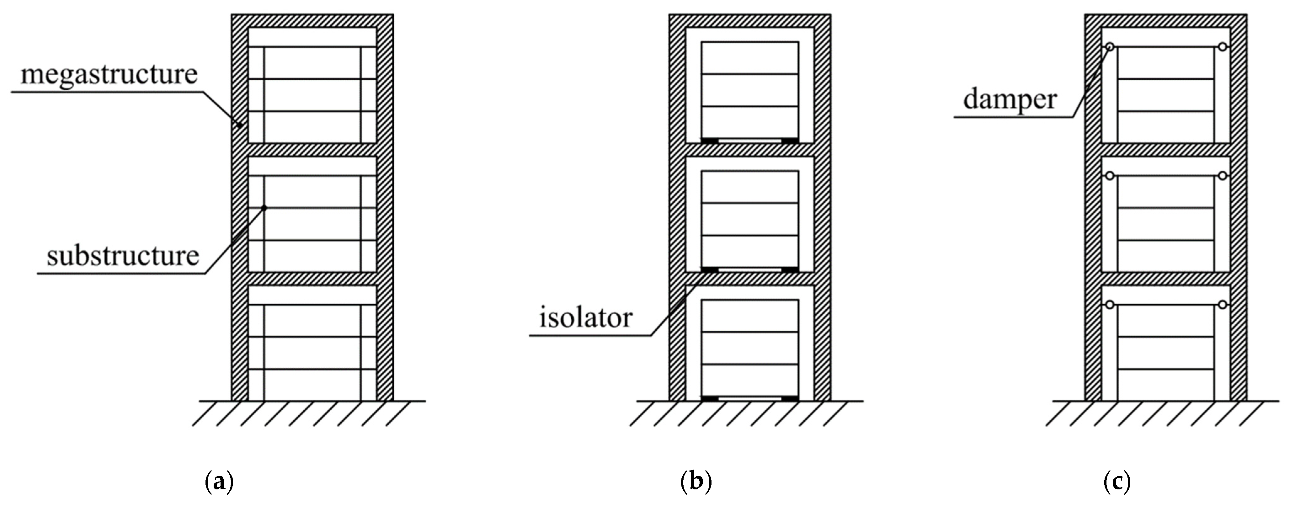
With the growth of the urban population, the demand for high-rise buildings is increasing. Mega-frame structure (MFS) is a type of structure that appeared in response to this demand. The megastructure of MFS consists of mega beams and mega columns. Solid web tubes or trusses are adopted as mega columns, and large hollow rectangular members or trusses are used as mega beams. The substructure is composed of ordinary beams and columns. Vertical loads on the substructure are transferred to the mega beams. The lateral stiffness of MFS depends on the stiffness of mega beams and columns. The substructures can be designed in various forms [1]. To reduce the dynamic response, Feng et al. [2] proposed an improved MFS called mega-frame with a vibration control substructure (MFVCS) with reference to the vibration control principle of tuned mass damper (TMD). MFVCS is also known as a mega-sub controlled structure. In this new structure, dampers or isolators were installed between the substructures and megastructures (Figure 1), and the function of the substructure is similar to that of the additional mass in TMD [3]. Many experiments and analyses showed that MFVCS has better response control ability than MFS [4,5,6,7]. Recent investigations have been devoted to further expanding and improving the design theory of MFVCS. Kalehsar et al. [8] compared the along-wind and crosswind responses of MFVCS and TMD, and investigated the influence of the mass ratio and stiffness ratio of the megastructure to the substructure on wind-induced vibration control of MFVCS. Fan et al. [9] calculated the failure path of MFVCS under random earthquake excitation by using the weighted rank–sum ratio method, and analyzed the weak members of the structure. Abdulhadi et al. [10] explored the appropriate stiffness ratio and mass ratio to reduce the seismic response of MFVCS. Shahzad et al. [11] proposed a modified MFVCS structure with isolators installed on mega columns.
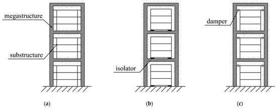
Figure 1.
Configurations of MFVCS. (a) MFS. (b) MFVCS with isolators. (c) MFVCS with dampers.
Since seismic design is an essential part of the design of MFVCS, seismic risk assessment is an issue worthy of attention. Seismic fragility analysis is an effective tool for this assessment, which provides an engineering indicator for decision-making in the design of new structures and the retrofitting of existing structures [12]. Seismic fragility analysis plays an important role in performance-based seismic engineering. There are three main types of fragility analysis methods: the expert opinion method, seismic damage investigation method, and analytical method [13]. The expert opinion method obtains the analysis results by collecting the evaluation opinions of experts, which is influenced by the expert experience. The seismic damage investigation method evaluates the fragility according to the actual seismic damage data, which is not suitable for areas lacking survey data. The analytical method uses numerical simulation to analyze the seismic risk, which is more commonly used than the first two methods. The fragility curves obtained from the fragility analysis can be used to assess the post-earthquake loss, which provides a basis for the seismic design of structures. In the past study [14], the incremental dynamic analysis (IDA) method was used to analyze the seismic fragility of MFVCS without considering the influence of structural uncertainties on seismic risk. In fact, although the record-to-record (RTR) variability is the main factor causing the variation of structural response [15,16], structural uncertainties may also affect the fragility curves [17]. In addition, the vibration control effect of MFVCS is related to the structural stiffness and damping device properties, and there are certain uncertainties in these parameters. Therefore, it is more reasonable to take the randomness of structural parameters into account in the seismic fragility analysis of MFVCS. Monte Carlo (MC) simulation can directly incorporate structural uncertainties into seismic fragility analysis, but needs a great number of calls to nonlinear time history analysis (NLTHA). Due to the complexity of MFVCS, repeated finite element analysis (FEA) will cause a huge computational burden.
Surrogate model approaches can give the approximations of structural responses and are very popular in reducing the computational cost. The dual surrogate model (DSM) framework is often used to describe the variability of optimization objectives in robust optimization, which employs two surrogate models to predict the mean and standard deviation of structural performance, respectively [18,19,20,21]. Towashiraporn [22] proposed the DSM-based seismic fragility analysis (DSM-SFA) method, in which DSM was introduced into seismic fragility analysis to tackle the RTR variability. DSM-SFA has been widely used in studies of structures subjected to seismic excitation, including bridges [23], base-isolated nuclear power plants [24], liquid storage tanks [25], and frame structures [26]. In addition, DSM has also been used to deal with problems considering other loads with RTR variabilities, such as wind [27], wave [28,29], and blast [30]. However, DSM-SFA has high requirements for the selection of the DoE used to build the surrogate models. The need for the number and distribution of experiment points is different for different structures, which is difficult to know before surrogate modeling. The one-shot sampling commonly used in the DSM framework may not obtain a suitable DoE, which will lead to the inaccuracy of fragility curves and waste of computing time.
In recent years, active learning (AL) sampling has been introduced into reliability analysis to improve the DoE [31,32]. The AL-based reliability analysis (AL-RA) methods usually adopt the Kriging model as the surrogate model. Taking advantage of the model’s ability to provide probability distributions of unknown values, the AL-RA methods select new samples sequentially from the candidate set to obtain the DoE, instead of choosing experiments by one-shot sampling. These methods can significantly reduce the calculation burden of MC simulation without much compromise on the accuracy of results, and have advantages in reliability analysis of large complex structures. However, the AL sampling strategies in AL-RA generally cannot be used in DSM-SFA. On the one hand, the prediction of each performance function in AL-RA is evaluated by one surrogate model, while two surrogate models are needed in DSM-SFA to estimate the seismic demand. On the other hand, reliability analysis is to calculate the failure probability of the structure, while seismic fragility analysis aims at obtaining the fragility curves which can describe the conditional failure probability corresponding to a given intensity measure (IM).
To accurately assess the seismic fragility of MFVCS in an efficient way, an improved DSM-SFA method based on AL is proposed. In the paper, the DSM framework for fragility analysis and the Kriging model are first reviewed. Then, the proposed method is described, and its effectiveness is validated by using an example. Finally, the finite element model of MFVCS is established and verified in OpenSeesPy, and the fragility analysis results of MFVCS and MFS considering structural uncertainties are compared.
2. DSM for Seismic Fragility Analysis
2.1. DSM-SFA
In DSM-SFA, both structural uncertainties and RTR variability are taken into account. Given the structural parameters s and IM value im, the engineering demand parameter (EDP) D of the structure under seismic load is assumed to be a random variable [24]. The mean and standard deviation of EDP vary with the structural parameters and IM. Usually, the lognormal EDP assumption [14,33] is adopted in seismic fragility analysis. To consider the RTR variability, multiple seismic records are required in structural analysis.
The surrogate model is constructed based on a DoE and the outputs , in which x(i) denotes an n-dimensional vector of input variables and denotes the function output of . Surrogate model approaches commonly used in DSM-SFA include the Kriging model and polynomial response surface.
The input variable vector x of the surrogate models in DSM-SFA consists of the structure parameters s and the IM variable im, i.e., . To establish the model, a group of experiments is first sampled in the space of x. At each experiment point, the mean and standard deviation of the logarithms of EDP results can be computed by carrying out NLTHA for all selected earthquakes. Then, the surrogate models of and can be constructed, respectively. The approximation of the unknown EDP is obtained [26] by:
where and are the predictions of and given by the surrogate models, respectively, and denotes a normally distributed variable whose mean is 0 and variance is .
Once the surrogate models of the standard deviation and mean are built, the failure probability for a given IM can be calculated by MC simulation, in which is used as a substitute for the true response to avoid performing NLTHA. Generally, a set of performance levels are considered in seismic fragility analysis, and each level corresponds to a limit state. The fragility curve corresponding to a performance level can be obtained by computing the failure probabilities for a series of IM values.
DSM-SFA requires much less computational time compared with the fragility analysis approach based on MC simulation, because the surrogate models of mean and standard deviation avoid repeated calls to FEA. However, since the DoE is usually obtained by one-shot sampling, the number of the selected experiments may not be appropriate. In addition, the generation of test samples used to verify the accuracy of the surrogate models also incurs additional computational costs.
2.2. Kriging Model
The Kriging model is an interpolation model composed of a parametric part and a nonparametric part [34], which is expressed as:
where denotes the unknown function to be fitted, is the vector of given basis functions, is the vector of the regression coefficients, and is a stationary Gaussian stochastic process with zero mean. The covariance of is:
where represents the process variance, and is the correlation function between the experiment points and . The anisotropic squared-exponential correlation function is usually adopted, which is described as:
where is the k-th component of the undetermined parameters θ, and is the k-th component of .
At point x, the prediction and the predicted variance are given by:
and
where R represents the m × m correlation matrix with component , is the correlation vector composed of the correlation function values between x and the experiment points, F denotes the m × p matrix of basis function values with component , , and and are the estimations of and .
and are calculated by:
and
The parameters θ can be determined by maximizing the log-likelihood function expressed as:
Kriging model can be classed among the realm of Gaussian process methods [35]. The unknown function value in the Kriging model is considered to follow a normal distribution as:
In this work, the ordinary Kriging model was adopted, where .
3. Proposed Seismic Fragility Analysis Method
3.1. Surrogate Models for Estimating the EDP
To overcome the difficulty of controlling the accuracy of surrogate models in DSM-SFA, the Kriging model is employed for surrogate modeling in the improved method. Although the Kriging model has been applied in existing literature on fragility analysis [23,36], its ability to analyze errors has not been utilized.
To be able to evaluate the error of the EDP approximation, Equation (1) is transformed into:
where v follows the standard normal distribution. It can be seen from Equation (10) that and , where and are the predicted standard deviations of and provided by the surrogate models. Then, when s, im, and v are fixed, the unknown value of logarithmic EDP follows the normal distribution and its predicted standard deviation can be obtained as:
Based on a group of MC samples , the probability that the EDP exceeds the h-th limit state for a given IM value im can be obtained by:
where is the threshold of EDP corresponding to the h-th limit state , and is an indicator function used to count the number of negative values. If the input is negative, the output of is 1; otherwise, it is equal to 0. Each sample in consists of the given im and randomly generated s and v.
3.2. AL Sampling
To refine the surrogate models adaptively, an AL sampling strategy was presented.
The initial experiments were uniformly selected using the Latin hypercube sampling (LHS) method [32] from the space of x between the lower and upper bounds of each variable. The lower and upper bounds of the i-th element in x can be , where denotes the inverse function of the probability distribution function of , and represents the probability distribution function of the standard normal distribution. The bounds of im can be the IM range concerned in the problem.
In the improvement of DoE, a candidate sample set needs to be first generated in the space of variables containing v, s, and im. It is worth noting that there is no need to perform a time history analysis on the candidate points. Then, the point which is most favorable for reducing the error of the result is selected from the candidate samples in terms of the learning function value of each point, and the values of and at this point are calculated. By adding to the DoE as a new test point, the surrogate models are updated once. The surrogate models can be gradually refined by choosing new experiments sequentially in this way.
It can be seen that the prediction of the sign of in Equation (13) depends on the accuracy of in the vicinity of the threshold . Thus, more attention should be paid to the accuracy of the predictions related to the limit states. The AL sampling strategy should be able to improve this accuracy. U function [32,37] is a widely used learning function in AL sampling. For the approximation of logarithmic EDP, the U function is described as:
Considering that a point with an approximate seismic demand close to a threshold and a large predicted error has a small U function value, the U function is used to identify the points that can reduce the error of near . In seismic fragility analysis, the accuracy of EDP approximation at multiple limit states needs to be considered. Consequently, the minimum U (MU) value at a sample for all limit states is treated as the learning function value of this sample, which is denoted as:
where Q is the number of performance levels. The point with the minimum MU value in the candidate set is taken as the new experiment, which is described as:
In the process of adding samples to DoE, the new experiment points will switch in the areas near these limit states as the accuracy of the surrogate models changes, so that the accuracy of EDP approximation in the vicinities of all thresholds will be improved together.
In AL-RA, if the U function value of a point is greater than 2, the probability of a wrong prediction of the safety state for this point is less than 2.3%. It is usually taken as the stopping condition of the AL-RA methods that the U function values of all candidate points are greater than 2 [37]. With reference to this condition, the proportion of candidate points with an MU value less than 2 is used in the proposed method as the indicator for the decision to stop sampling, which is expressed as:
where denotes the number of points whose MU value is less than 2 in the candidate sample set. When is less than a certain tolerance ζ, the sampling of new experiments can be stopped. ζ is taken as 0.02 in this research.
The selection of candidate points is performed according to the probability distribution of variables, similar to the selection of MC samples. In the generation of the candidate set, im is regarded as a uniformly distributed variable. LHS is employed for sampling to avoid excessive aggregation of candidate points. Based on a group of points uniformly sampled in the space of , the candidate set can be obtained by the transformation [17] as:
3.3. Computational Process of Seismic Fragility Analysis
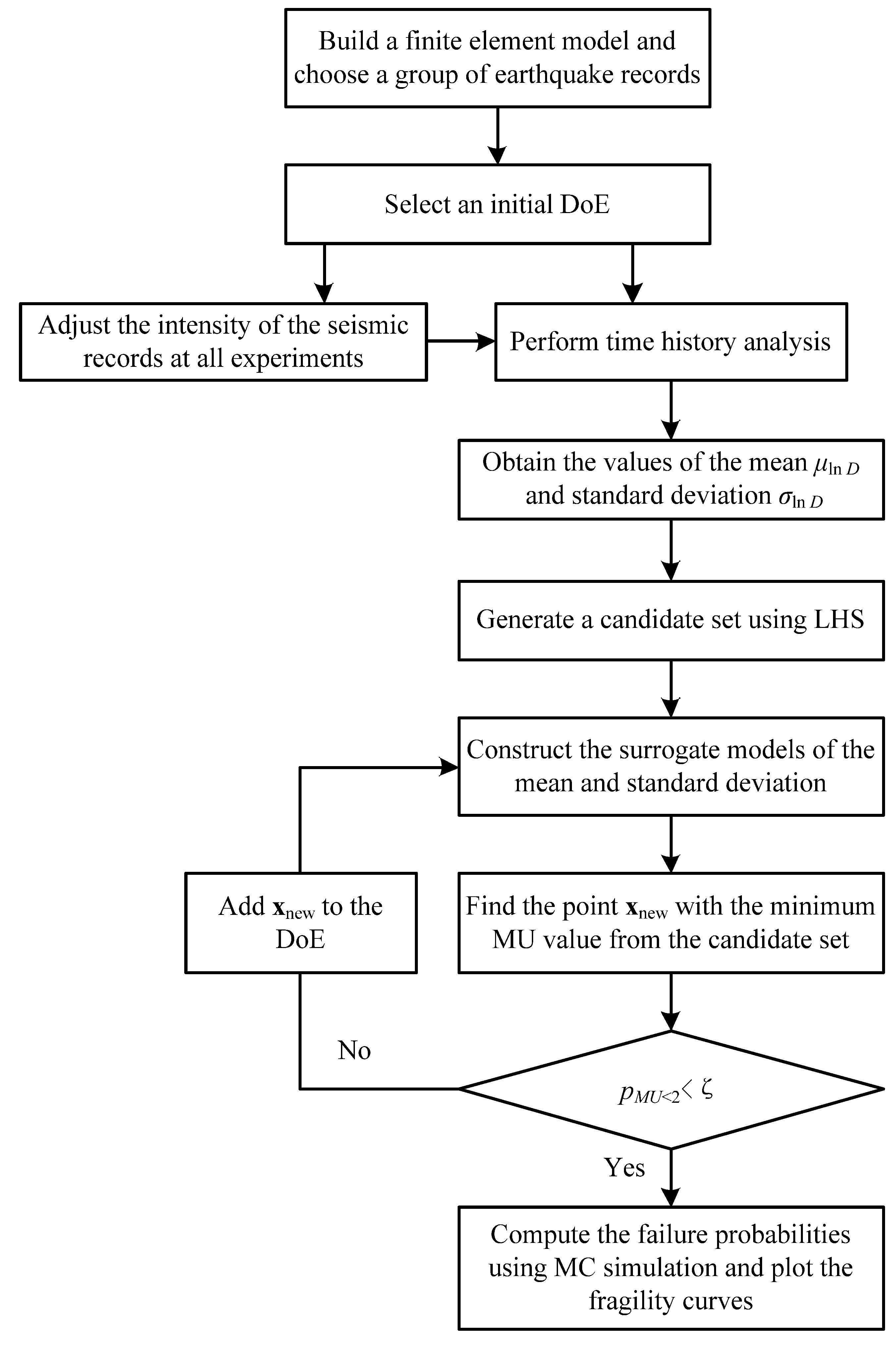
The proposed seismic fragility analysis method can be implemented as the following process:
Step 1: Build a finite element model of the structure and choose a group of earthquake records.
Step 2: Select a DoE containing several experiments in the space of using LHS, and carry out NLTHA to compute the mean and standard deviation of the logarithmic EDP for each experiment.
Step 3: Generate a candidate set consisting of r samples (r = 1000 in this work) in the space of using LHS according to Equation (18).
Step 4: Based on the DoE, establish the surrogate models of the mean and standard deviation using Kriging model.
Step 5: Find the point with the minimum MU value from the candidate samples in terms of Equation (16). If the stopping condition < ζ (ζ is taken as 0.02) is unsatisfied, calculate the values of and at the point , add this point to the DoE, and return to step 4; otherwise, go to the next step.
Step 6: Compute the failure probabilities of the structure for a series of IM values using MC simulation with Equation (13), and plot the results as fragility curves.
The above process is drawn as a flowchart in Figure 2.

Figure 2.
Flowchart of seismic fragility analysis.
3.4. Validation Example
To demonstrate the effectiveness and feasibility of the proposed method, a three-dimensional five-storey steel frame was studied, and the results were compared with those of the MC simulation and DSM-SFA methods. As the calculation time is mainly spent on NLTHA, the calculation efficiency was evaluated by , the number of calls to FEA, which is equal to the number of experiments in DoE.
It was assumed that the site classification was II, and the seismic fortification intensity was 8. According to the requirements of seismic records for time history analysis in the current Chinese code for seismic design of buildings (GB50011-2010) [38], 12 records corresponding to the site condition were selected, which are listed in Table 1. The design spectrum from the seismic code and the response spectra of the selected earthquakes are shown in Figure 3. The maximum inter-storey drift angle is a widely accepted parameter for evaluating structural damage, and it was employed as EDP. The peak ground acceleration (PGA) is a commonly used index to measure the ground motion intensity, and it was adopted as IM in this study. Three performance levels, namely, immediate occupancy, life safety, and collapse prevention, were considered. With reference to the control target of the maximum inter-storey drift angle of steel structures corresponding to different failure states in GB50011-2010, the thresholds of these three performance levels were taken as = 1/200, = 1/100, and = 1/50, respectively.

Table 1.
Seismic records.
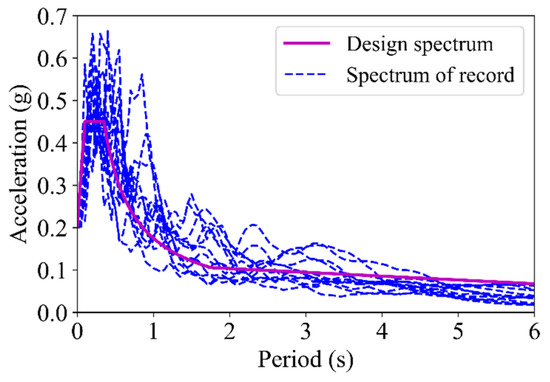
Figure 3.
Spectra of the earthquakes.
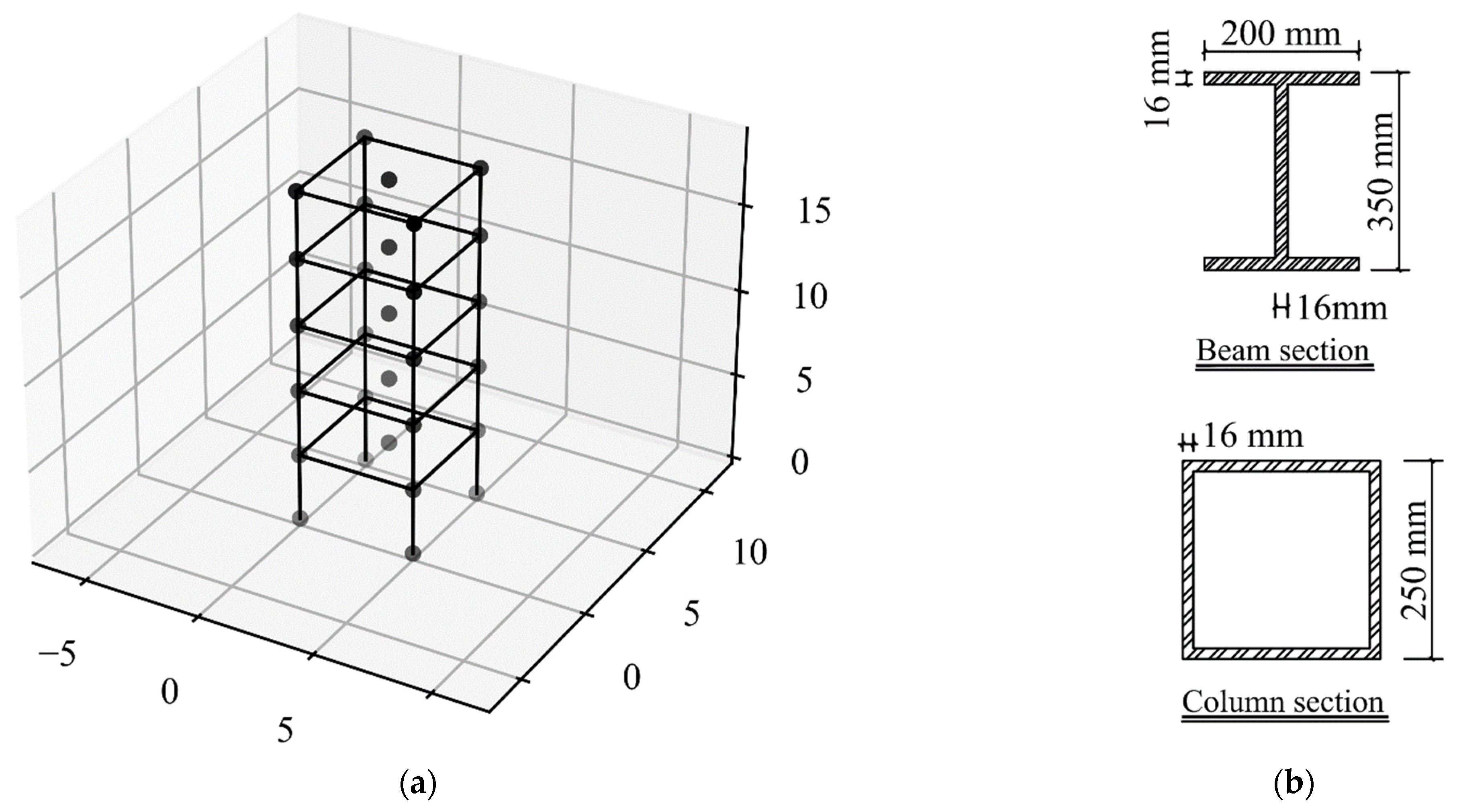
The finite element model of the structure was constructed in OpenSeesPy (Figure 4a). The storey height was 3.8 m, and the span of each beam was 5 m. The density of steel was 7850 kg/m3. The cross-section information of beams and columns is shown in Figure 4b. The displacement-based beam–column element was adopted to model the beams and columns. The stress-strain behavior of steel was simulated by the Steel02 material (uniaxial Giuffre–Menegotto–Pinto material with isotropic strain hardening), where the strain-hardening ratio B was 0.02 and the three parameters controlling the transition of steel from elastic stage to hardening stage were 18, 0.925 and 0.15, respectively [39]. The material model is shown in Figure 5, where and represent the yield strength and initial elastic modulus of steel. The vertical load of 7 kN/m2 was uniformly distributed on each floor. The slabs were modeled through a diaphragm constraint at each floor [40]. Rayleigh damping model was used in dynamic analysis.
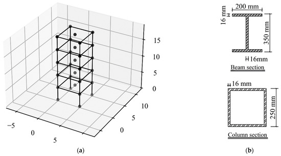
Figure 4.
Five-storey steel frame. (a) Finite element model. (b) Cross-sections.
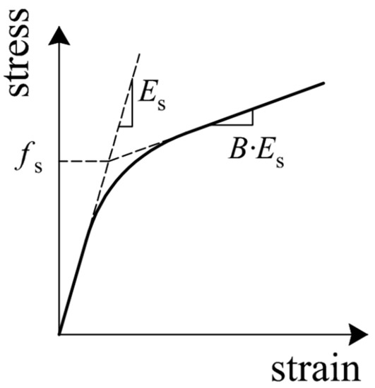
Figure 5.
Stress-strain behavior of steel.
In the aspect of structural uncertainties, the randomness of structural damping ratio ξ [41,42], yield strength , and initial elastic modulus were considered. The probability distribution, mean, and coefficient of variation (CoV) of the structural parameters are listed in Table 2.
Table 2.
Statistical properties of the structural parameters.
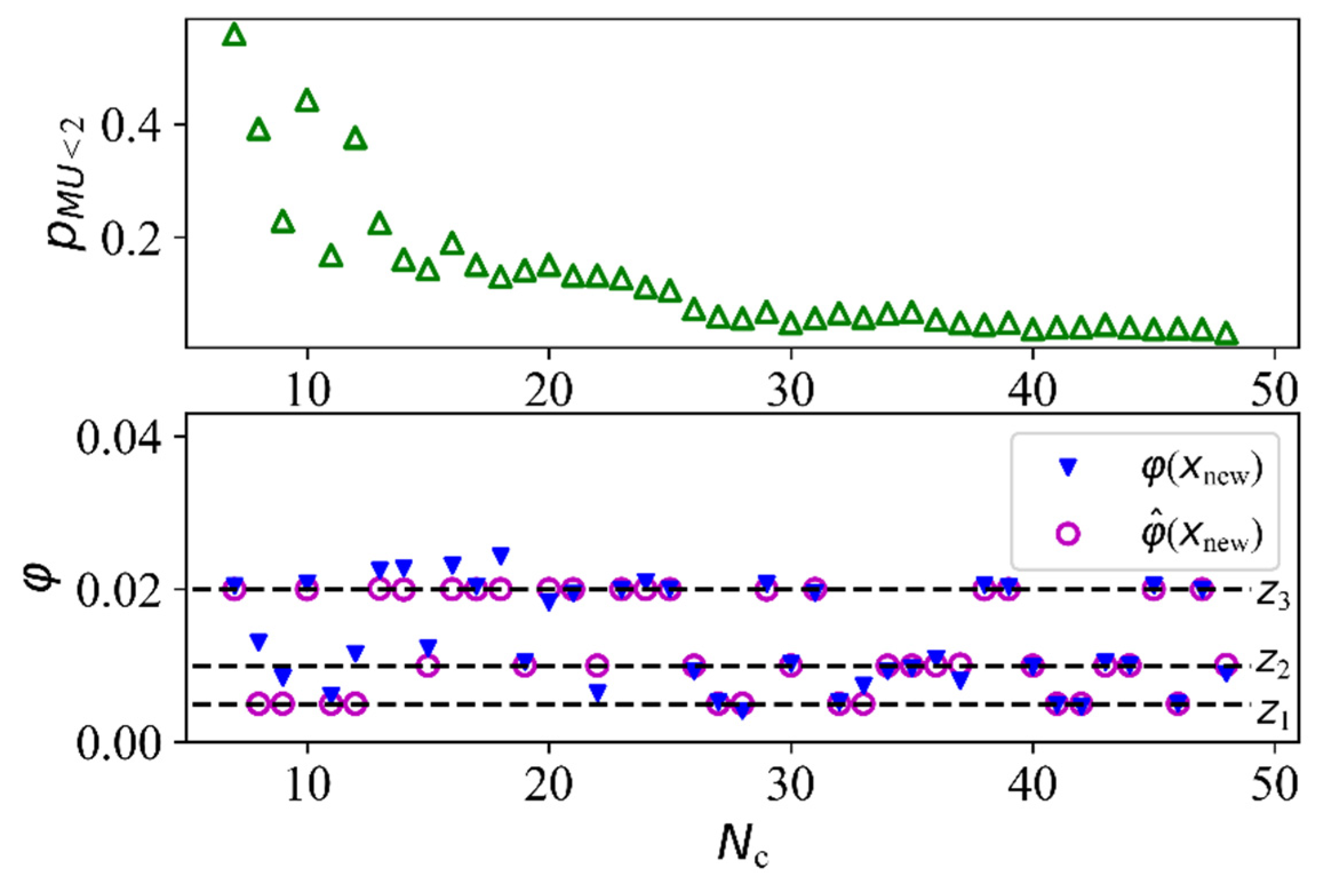
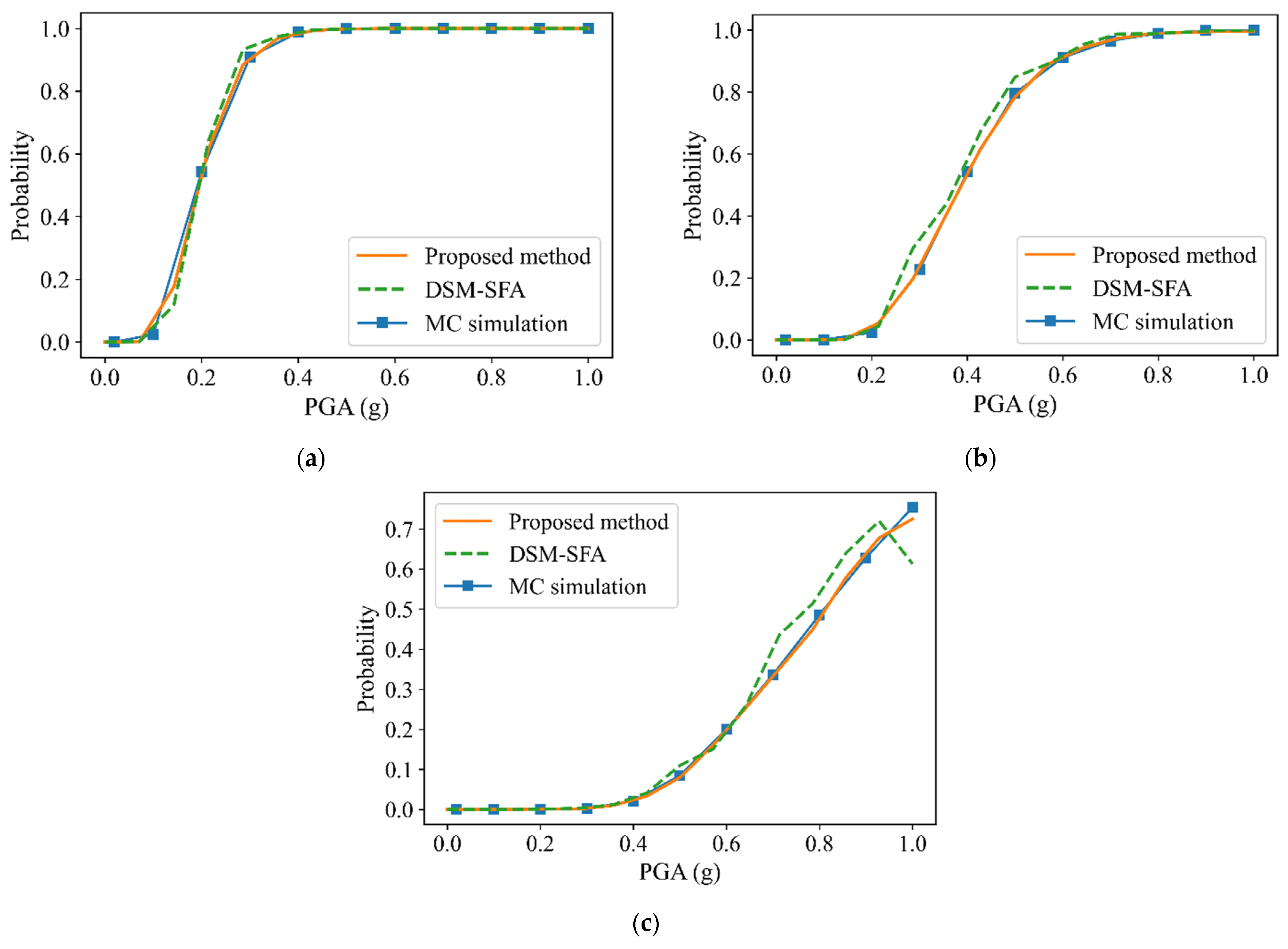
The seismic fragility of the structure was analyzed using the proposed method, in which 6 initial experiments were selected and 42 samples were added to the DoE by AL sampling. In the process of AL sampling, the maximum inter-storey drift angle and the approximation at the new samples are shown in Figure 6. It can be observed that the EDP approximations of the new points are mainly located in the vicinities of the thresholds of limit states. As the number of experiments in DoE increased, decreased gradually. To validate the accuracy and efficiency of the developed method, MC simulation and DSM-SFA were used to calculate the fragility curves. The curves obtained by these three approaches are shown in Figure 7.
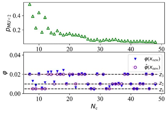
Figure 6.
The seismic demand of the added samples.
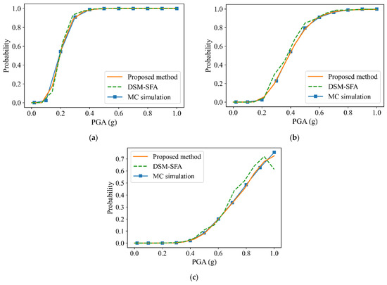
Figure 7.
Fragility curves obtained using different approaches. (a) Immediate occupancy. (b) Life safety. (c) Collapse prevention.
In the calculation of MC simulation, the MC samples were selected by LHS, and the number of samples was 1000. The failure probabilities of the structure were calculated for PGAs of 0.02, 0.1, 0.2, …, 1.0 g, respectively, and the number of calls to FEA to obtain the fragility curves was 1000 × 11. The fragility curves plotted by the proposed procedure had little difference from those by MC simulation, and the value of the former was only 0.4% of that of the latter. Since MC simulation is a very accurate reliability method, the closeness of the two results verifies the accuracy of the proposed method.
In the calculation of the DSM-SFA method, the number of the experiments was made equal to the value in the calculation of the proposed method, and the Kriging model was used for surrogate modeling. Although the numbers of calls to FEA in the analyses of the two methods are the same, the fragility curves obtained by the DSM-SFA method had obvious errors. This indicates that the proposed method needs less computation than the DSM-SFA method to obtain sufficiently accurate results, which verifies its efficiency. Compared with the traditional DSM framework for fragility analysis, this method gives full play to the ability of the Kriging model to predict errors and avoids overreliance on one-shot sampling.
4. Seismic Fragility Analysis of MFVCS
In this section, the developed method was applied to MFVCS. The influence of structural uncertainties on the fragility curves of MFVCS was studied, and the fragility of MFVCS and MFS was compared.
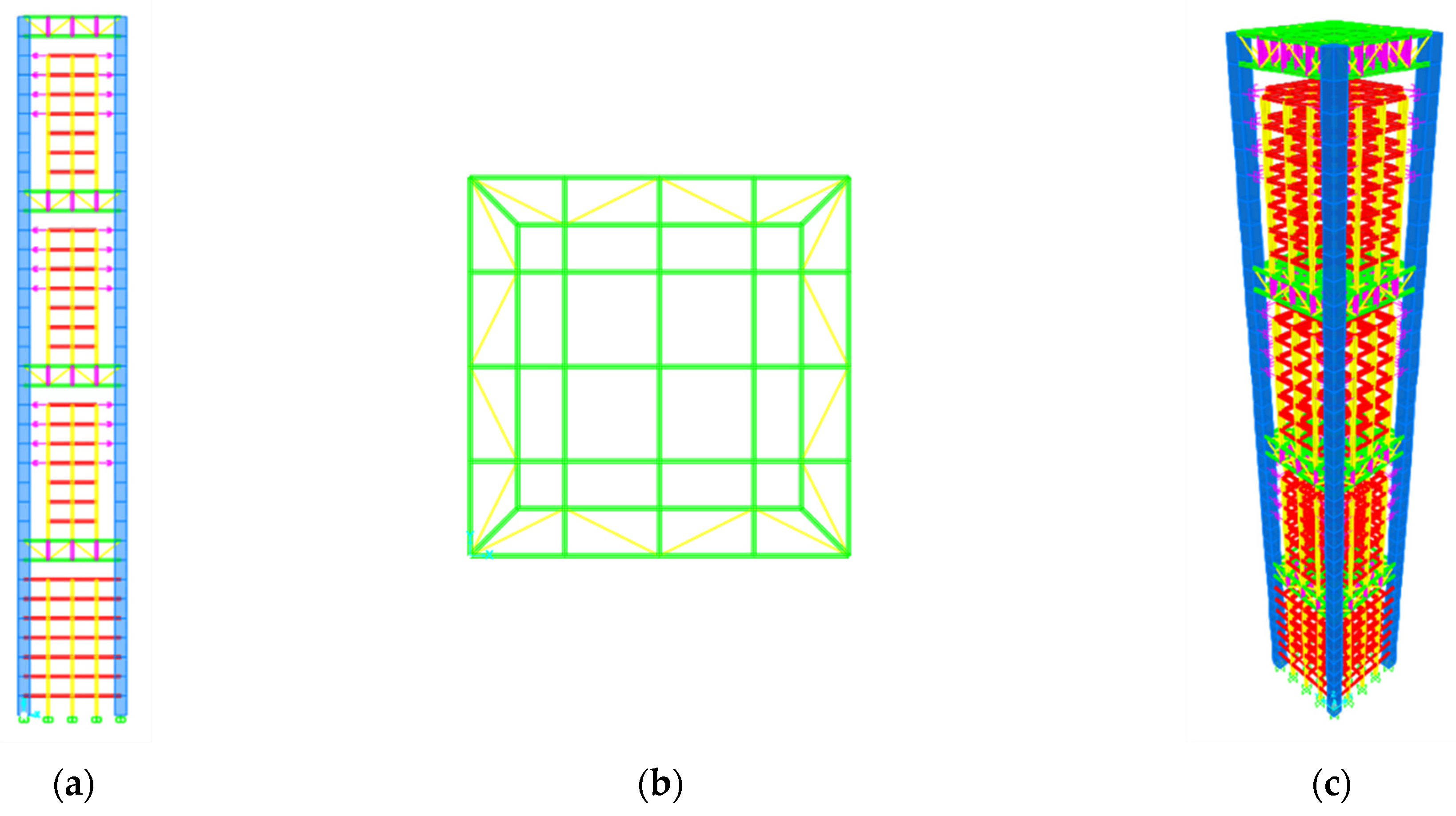
4.1. Establishment of Finite Element Model
The components of MFVCS in this research were arranged with reference to the experimental model in previous studies [43,44] and the configuration of the structure is shown in Figure 8a. The structure has four mega storeys. The beam span and storey height of the substructures were 5 and 4 m, respectively. The cross-section information of the members is listed in Table 3. The yield strength and the elastic modulus of steel were 300 MPa and 200 GPa. The dead load (including the self-weight of the slab) and live load on the slab surface were 4 and 2 kN/m2. Viscous dampers connected to the mega columns were installed on the substructures of the second, third, and fourth mega storeys. In this work, the damper constitutive law [45,46] is described in the form:
where represents the damper resisting force, denotes the damping coefficient, α represents the velocity exponent, denotes the velocity between the damper’s end, and is the sign extractor operator.
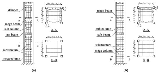
Figure 8.
Schematics of MFS and MFVCS. (a) MFVCS. (b) MFS.
Table 3.
Member section information.
The finite element model of MFVCS was built in OpenSeesPy. The material model of steel and the element used to model beams and columns were the same as those in the previous section. The hysteretic response of the damper was simulated using the Maxwell material model.
To verify the finite element model, another model was established in SAP2000 (Figure 9). The modal analysis of two finite element models was carried out, and the information of the first six natural vibration periods is listed in Table 4. The calculation results of the two software were very close. Therefore, the finite element model in this study could be considered correct and could be used for subsequent research.
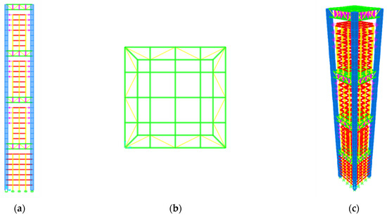
Figure 9.
Finite element model of MFVCS. (a) Elevation View. (b) Plan View. (c) 3D View.
Table 4.
Modal analysis results.
4.2. Comparison of Results
In the fragility analysis of MFVCS, the uncertainties of material properties and damper parameters [45] were taken into account. The statistical properties of random variables are shown in Table 5. The same seismic records as those in the validation example were used for NLTHA.
Table 5.
Statistical properties of random variables.
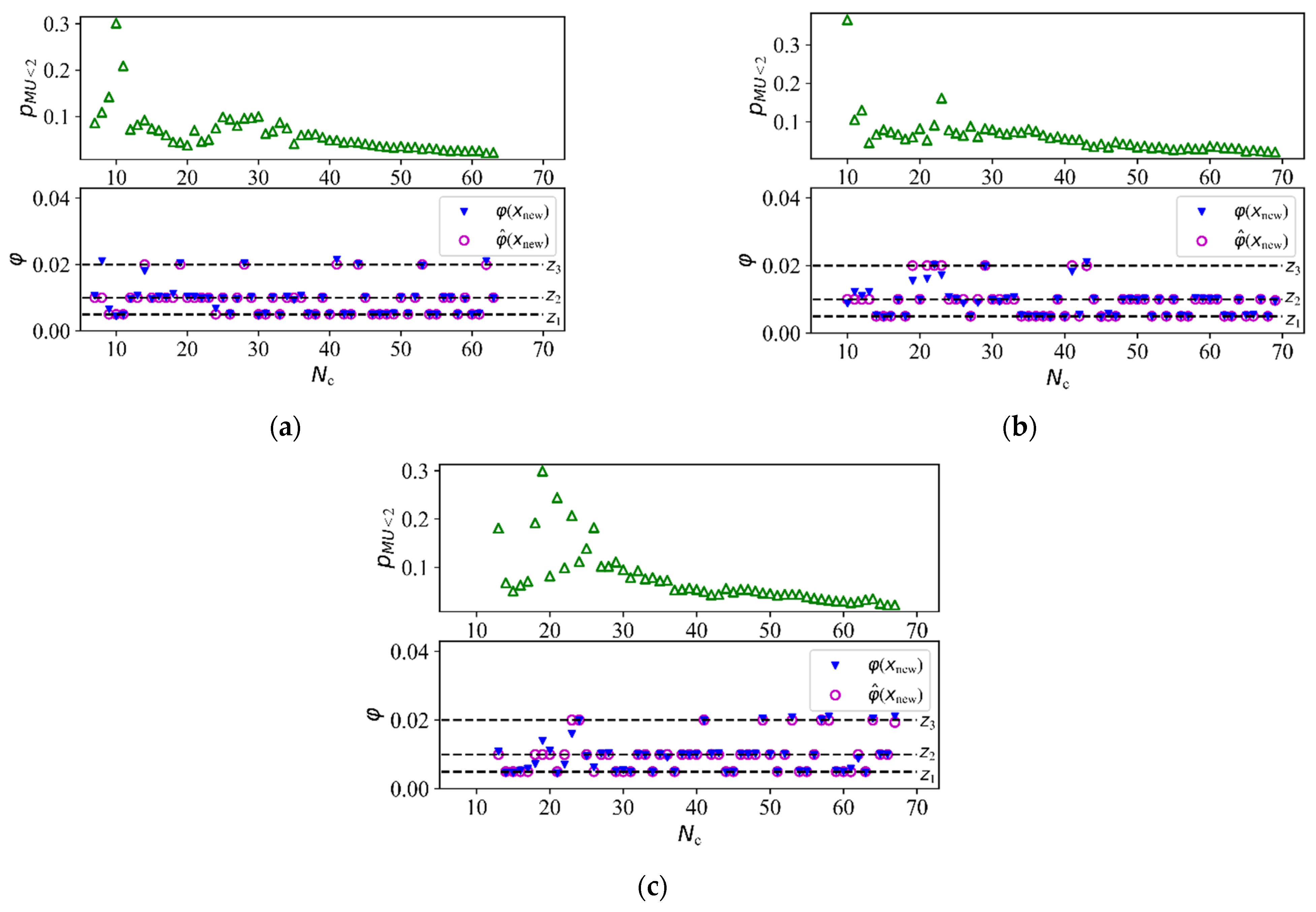
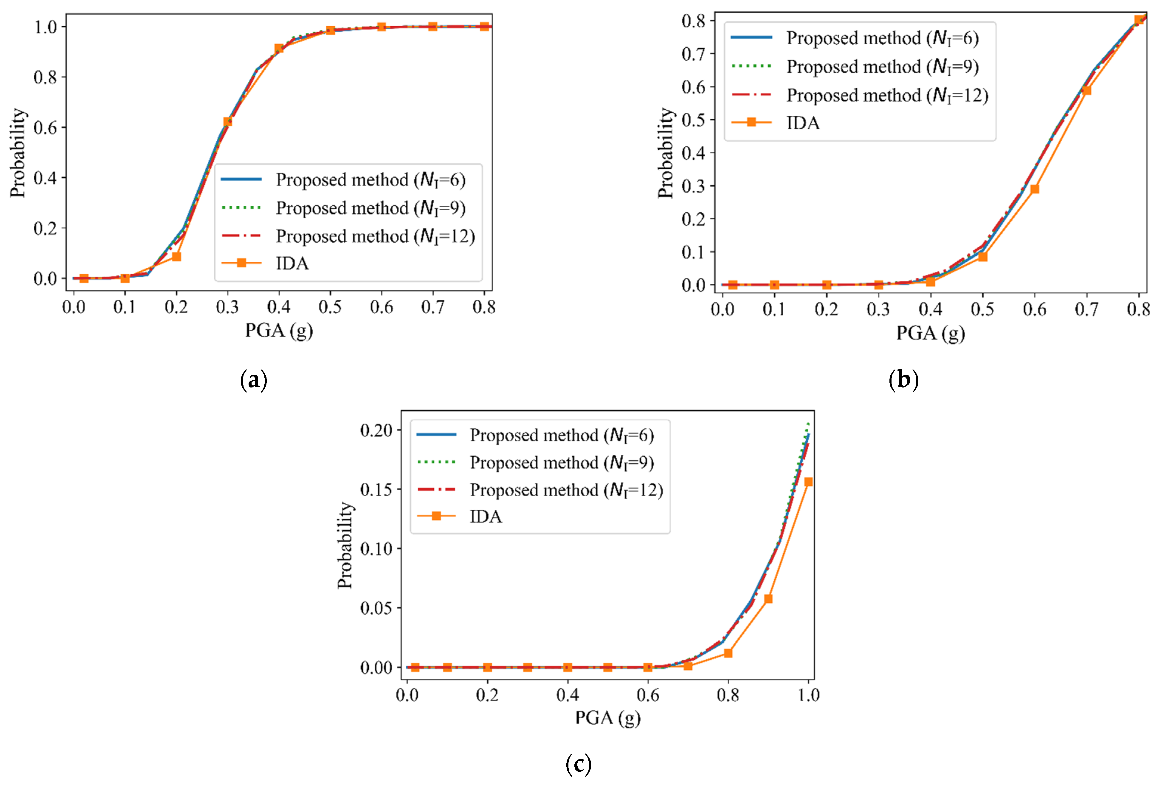
The seismic fragility of MFVCS was calculated using the proposed procedure in three different cases, in which the numbers of initial experiments NI were 6, 9, and 12, respectively. The values of , , and of the new samples in the sampling process are plotted in Figure 10. The fragility curves are plotted in Figure 11. The results of the three analyses were in good agreement, which indicates that the proposed method can obtain the fragility curves stably.
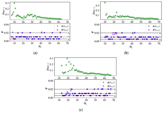
Figure 10.
The seismic demand of the added samples of MFVCS. (a) NI = 6. (b) NI = 9. (c) NI = 12.
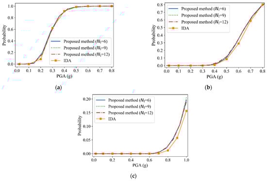
Figure 11.
Fragility curves of MFVCS obtained using different approaches. (a) Immediate occupancy. (b) Life safety. (c) Collapse prevention.
To study the effect of structural randomness on the seismic fragility of MFVCS, the fragility curves were calculated by the IDA method neglecting model uncertainty. The CoV of each parameter was treated as 0. The probability of EDP exceeding for a given IM value im calculated by IDA [14] is:
The results are also drawn in Figure 11. For the immediate occupancy level, there is not much difference between the results corresponding to considering and ignoring the model uncertainty. For the collapse prevention level, the difference between the two results is obvious. It shows that structural uncertainties can cause significant variation of the fragility curve corresponding to the collapse prevention level of MFVCS.
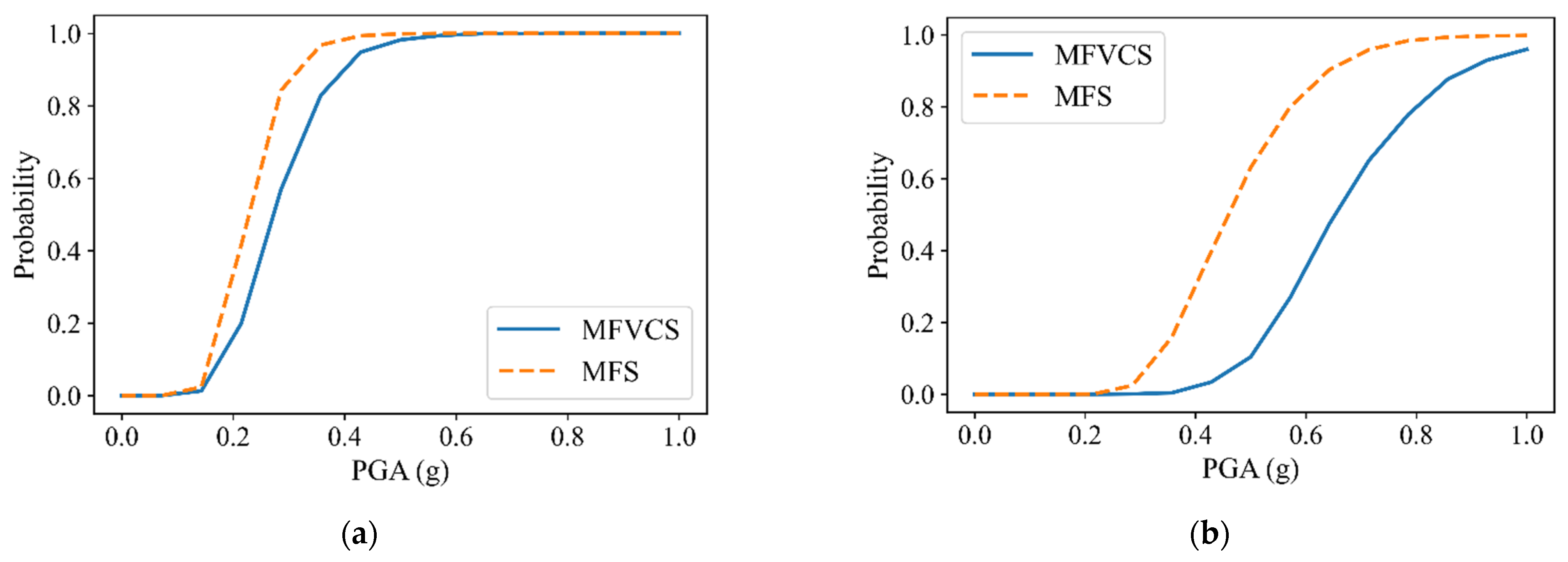
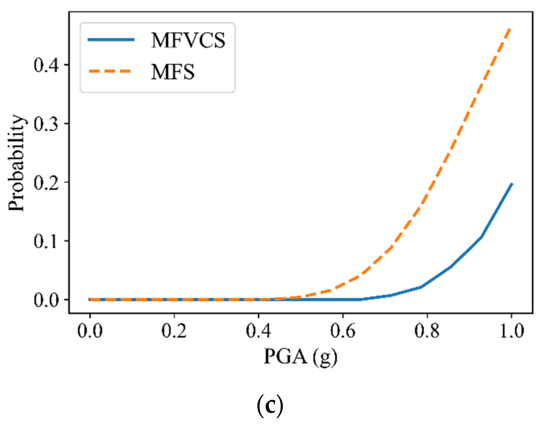
The fragility of MFS was also analyzed by the proposed method. The component arrangement of MFS is shown in Figure 8b. The member cross-sections were the same as those of MFVCS. Due to the absence of dampers, the parameters of the damping device were not considered in the fragility analysis. The statistical properties of other random parameters were the same as those of MFVCS. The number of calls to FEA in the calculation was 38. The fragility curves are shown in Figure 12. By comparing the curves of the two structures, it can be found that the failure probability of MFS is obviously higher than that of MFVCS under the same PGA, indicating that MFVCS is less vulnerable than MFS. Therefore, compared with MFS, MFVCS has better seismic performance. Compared with the previous studies on MFVCS based on IDA [14,47], this method can incorporate the randomness of structural parameters into fragility analysis, which provides more accurate reliability information for the seismic design of MFVCS.
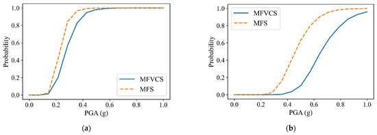
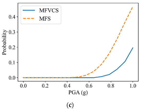
Figure 12.
Fragility curves of MFS and MFVCS. (a) Immediate occupancy. (b) Life safety. (c) Collapse prevention.
5. Conclusions
To save the computational time of the seismic fragility analysis of MFVCS considering structural uncertainties, an improved DSM-SFA method was proposed in this paper. This method modifies the way of estimating the seismic response in DSM-SFA, so that the predicted error of the approximation can be obtained by the Kriging model. Based on the ability to predict errors, an AL sampling strategy is presented to adaptively select an appropriate DoE, thus improving the efficiency and accuracy of the DSM framework for fragility analysis. The proposed method is generic in nature and can be used for other structures under seismic load.
An example was analyzed by using different approaches to verify the effectiveness and feasibility of the proposed procedure. It has been observed that the calculation cost of this method is far less than that of MC simulation and the fragility curves of the two methods are very close. With the same number of calls to FEA, the errors of the fragility curves obtained by the DSM-SFA method are larger than those by the proposed method. The results show that the developed method is efficient and accurate.
The finite element model of MFVCS was established, and the proposed procedure was applied to its seismic fragility analysis. For the cases with different initial points, the analysis results were in good agreement, which indicates that this method can obtain the fragility curves stably. The comparison between the results of IDA and the developed method reveals that structural uncertainties have an effect on the fragility curves, especially the curve of the collapse prevention level. In addition, the fragility curves of MFS and MFVCS were compared in this paper, which shows that the damage probability of MFVCS is smaller than that of MFS under the same PGA and MFVCS has better seismic performance.
The proposed procedure provides a foundation for our future study on reliability-based design optimization of MFVCS considering the RTR variability of wind load.
Author Contributions
Conceptualization, Y.X.; methodology, Y.X.; software, Y.X.; validation, F.Y., B.F., M.M.S. and X.W.; formal analysis, Y.X.; investigation, Y.X.; resources, Y.X.; data curation, F.Y., B.F., M.M.S. and X.W.; writing—original draft preparation, Y.X.; writing—review and editing, F.Y.; visualization, Y.X.; supervision, X.Z.; project administration, X.Z.; funding acquisition, X.Z. All authors have read and agreed to the published version of the manuscript.
Funding
This work was supported by the National Natural Science Foundation of China under Grant No. 51078311.
Institutional Review Board Statement
Not applicable.
Informed Consent Statement
Not applicable.
Data Availability Statement
The data used to support the findings of this study are available from the corresponding author upon request.
Conflicts of Interest
The authors declare no conflict of interest.
Abbreviation
| Abbreviation | Meaning |
| MFS | mega-frame structure |
| MFVCS | mega-frame with vibration control substructure |
| TMD | tuned mass damper |
| DSM | dual surrogate model |
| IDA | incremental dynamic analysis |
| IM | intensity measure |
| EDP | engineering demand parameter |
| AL | active learning |
| DoE | design of experiments |
| CoV | coefficient of variation |
| FEA | finite element analysis |
| LHS | Latin hypercube sampling |
| PGA | peak ground acceleration |
| NLTHA | nonlinear time history analysis |
References
- Zhang, X.A.; Qin, X.; Cherry, S.; Lian, Y.; Zhang, J.; Jiang, J. A new proposed passive mega-sub controlled structure and response control. J. Earthq. Eng. 2009, 13, 252–274. [Google Scholar] [CrossRef]
- Feng, M.Q.; Mita, A. Vibration control of tall buildings using mega subconfiguration. J. Eng. Mech. 1995, 121, 1082–1088. [Google Scholar] [CrossRef] [Green Version]
- Qin, X.; Zhang, X.A.; Sheldon, C. Study on semi-active control of mega-sub controlled structure by MR damper subject to random wind loads. Earthq. Eng. Eng. Vib. 2008, 7, 285–294. [Google Scholar] [CrossRef]
- Jiang, Q.; Wang, H.Q.; Ye, X.G.; Chong, X.; Feng, Y.L.; Wang, J.; Yao, H.T. Shaking table model test of a mega-frame with a vibration control substructure. Struct. Des. Tall Spec. Build. 2020, 29, e1742. [Google Scholar] [CrossRef]
- Abdulhadi, M.; Zhang, X.A.; Fan, B.; Moman, M. Design, Optimization and Nonlinear Response Control Analysis of the Mega Sub-Controlled Structural System (MSCSS) Under Earthquake Action. J. Earthq. Tsunami 2020, 14, 2050013. [Google Scholar] [CrossRef]
- Liang, Q.; Li, L.; Yang, Q. Seismic analysis of the tuned—Inerter—Damper enhanced mega-sub structure system. Struct. Control. Health Monit. 2021, 28, e2658. [Google Scholar] [CrossRef]
- Xiao, Y.J.; Yue, F.; Zhang, X.A.; Shahzad, M.M. Aseismic Optimization of Mega-sub Controlled Structures Based on Gaussian Process Surrogate Model. KSCE J. Civ. Eng. 2022, 26, 2246–2258. [Google Scholar] [CrossRef]
- Kalehsar, H.E.; Khodaie, N. Wind-induced vibration control of super-tall buildings using a new combined structural system. J. Wind. Eng. Ind. Aerodyn. 2018, 172, 256–266. [Google Scholar] [CrossRef]
- Fan, B.; Zhang, X.A.; Abdulhadi, M.; Moman, M.; Wang, Z. Seismic behavior of MSCSS based on story drift and failure path. Lat. Am. J. Solids Struct. 2021, 18, e411. [Google Scholar] [CrossRef]
- Abdulhadi, M.; Zhang, X.A.; Fan, B.; Moman, M. Substructure design optimization and nonlinear responses control analysis of the mega-sub controlled structural system (MSCSS) under earthquake action. Earthq. Eng. Eng. Vib. 2021, 20, 687–704. [Google Scholar] [CrossRef]
- Shahzad, M.M.; Zhang, X.A.; Wang, X.; Abdulhadi, M.; Wang, T.; Xiao, Y.J. Response control analysis of a new mega-subcontrolled structural system (MSCSS) under seismic excitation. Struct. Des. Tall Spec. Build. 2022, 2022, e1935. [Google Scholar] [CrossRef]
- Park, J.; Towashiraporn, P. Rapid seismic damage assessment of railway bridges using the response-surface statistical model. Struct. Saf. 2014, 47, 1–12. [Google Scholar] [CrossRef]
- Gentile, R.; Galasso, C. Gaussian process regression for seismic fragility assessment of building portfolios. Struct. Saf. 2020, 87, 101980. [Google Scholar] [CrossRef]
- Wang, X.; Shahzad, M.M.; Shi, X. Fragility analysis and collapse margin capacity assessment of mega-sub controlled structure system under the excitation of mainshock-aftershock sequence. J. Build. Eng. 2022, 49, 104080. [Google Scholar] [CrossRef]
- Nazri, F.M.; Kian Yern, C.; Kassem, M.M.; Farsangi, E.N. Assessment of structure-specific fragility curves for soft storey buildings implementing IDA and SPO approaches. Int. J. Eng. 2018, 31, 2016–2021. [Google Scholar] [CrossRef]
- Bao, X.; Jin, L.; Liu, J.; Xu, L. Framework for the mainshock-aftershock fragility analysis of containment structures incorporating the effect of mainshock-damaged states. Soil Dyn. Earthq. Eng. 2022, 153, 107072. [Google Scholar] [CrossRef]
- Asgarian, B.; Ordoubadi, B. Effects of structural uncertainties on seismic performance of steel moment resisting frames. J. Constr. Steel Res. 2016, 120, 132–142. [Google Scholar] [CrossRef]
- Lin, D.K.; Tu, W. Dual response surface optimization. J. Qual. Technol. 1995, 27, 34–39. [Google Scholar] [CrossRef]
- Fang, J.; Gao, Y.; Sun, G.; Xu, C.; Li, Q. Multi-objective robust design optimization of fatigue life for a truck cab. Reliab. Eng. Syst. Saf. 2015, 135, 1–8. [Google Scholar] [CrossRef]
- Wu, Y.; Li, W.; Fang, J.; Lan, Q. Multi-objective robust design optimization of fatigue life for a welded box girder. Eng. Optim. 2018, 50, 1252–1269. [Google Scholar] [CrossRef]
- Qiu, N.; Jin, Z.; Liu, J.; Fu, L.; Chen, Z.; Kim, N.H. Hybrid multi-objective robust design optimization of a truck cab considering fatigue life. Thin-Walled Struct. 2021, 162, 107545. [Google Scholar] [CrossRef]
- Towashiraporn, P. Building Seismic Fragilities Using Response Surface Metamodels. Ph.D. Thesis, Georgia Institute of Technology, Atlanta, CA, USA, 2004. [Google Scholar]
- Zhang, Y.; Wu, G. Seismic vulnerability analysis of RC bridges based on Kriging model. J. Earthq. Eng. 2019, 23, 242–260. [Google Scholar] [CrossRef]
- Perotti, F.; Domaneschi, M.; De Grandis, S. The numerical computation of seismic fragility of base-isolated nuclear power plants buildings. Nucl. Eng. Des. 2013, 262, 189–200. [Google Scholar] [CrossRef]
- Saha, S.K.; Matsagar, V.; Chakraborty, S. Uncertainty quantification and seismic fragility of base-isolated liquid storage tanks using response surface models. Probabilistic Eng. Mech. 2016, 43, 20–35. [Google Scholar] [CrossRef]
- Xiao, Y.; Ye, K.; He, W. An improved response surface method for fragility analysis of base-isolated structures considering the correlation of seismic demands on structural components. Bull. Earthq. Eng. 2020, 18, 4039–4059. [Google Scholar] [CrossRef]
- Datta, G.; Bhattacharjya, S.; Chakraborty, S. Efficient reliability-based robust design optimization of structures under extreme wind in dual response surface framework. Struct. Multidiscip. Optim. 2020, 62, 2711–2730. [Google Scholar] [CrossRef]
- Datta, G.; Bhattacharjya, S.; Chakraborty, S. Robust design of offshore jacket platform structure under random wave in dual response surface framework. Struct. Infrastruct. Eng. 2021, 17, 887–901. [Google Scholar] [CrossRef]
- Majumder, S.; Datta, G.; Bhattacharjya, S. A dual response surface-based efficient fragility analysis approach of offshore structures under random wave load. Appl. Math. Model. 2021, 98, 680–700. [Google Scholar] [CrossRef]
- Datta, G.; Bhattacharjya, S.; Chakraborty, S. A metamodeling-based robust optimisation approach for structures subjected to random underground blast excitation. Structures 2021, 33, 3615–3632. [Google Scholar] [CrossRef]
- Guo, Q.; Liu, Y.; Zhao, Y.; Li, B.; Yao, Q. Improved resonance reliability and global sensitivity analysis of multi-span pipes conveying fluid based on active learning Kriging model. Int. J. Press. Vessel. Pip. 2019, 170, 92–101. [Google Scholar] [CrossRef]
- Guo, Q.; Liu, Y.; Chen, B.; Yao, Q. A variable and mode sensitivity analysis method for structural system using a novel active learning Kriging model. Reliab. Eng. Syst. Saf. 2021, 206, 107285. [Google Scholar] [CrossRef]
- Xiao, Y.J.; Yue, F.; Zhang, X.A. Seismic Fragility Analysis of Structures Based on Adaptive Gaussian Process Regression Metamodel. Shock Vib. 2021, 2021, 7622130. [Google Scholar] [CrossRef]
- Qin, S.; Zhou, Y.L.; Cao, H.; Wahab, M.A. Model updating in complex bridge structures using kriging model ensemble with genetic algorithm. KSCE J. Civ. Eng. 2018, 22, 3567–3578. [Google Scholar] [CrossRef]
- Preuss, R.; Von Toussaint, U. Global optimization employing Gaussian process-based Bayesian surrogates. Entropy 2018, 20, 201. [Google Scholar] [CrossRef] [PubMed]
- Phan, H.N.; Paolacci, F.; Corritore, D.; Tondini, N.; Bursi, O.S. A Kriging-Based Surrogate Model for Seismic Fragility Analysis of Unanchored Storage Tanks. In Pressure Vessels and Piping Conference; ASME: San Antonio, TX, USA, 2019; p. V008T08A024. [Google Scholar] [CrossRef]
- Xiao, Y.J.; Yue, F.; Wang, X.; Zhang, X.A. Reliability-Based Design Optimization of Structures Considering Uncertainties of Earthquakes Based on Efficient Gaussian Process Regression Metamodeling. Axioms 2022, 11, 81. [Google Scholar] [CrossRef]
- GB 50011-2010; Code for Seismic Design of Buildings. Ministry of Construction of the People’s Republic of China: Beijing, China, 2010. (In Chinese)
- Jin, S.; Du, H.; Bai, J. Seismic performance assessment of steel frame structures equipped with buckling-restrained slotted steel plate shear walls. J. Constr. Steel Res. 2021, 182, 106699. [Google Scholar] [CrossRef]
- Barbato, M.; Gu, Q.; Conte, J.P. Probabilistic push-over analysis of structural and soil-structure systems. J. Struct. Eng. 2010, 136, 1330–1341. [Google Scholar] [CrossRef] [Green Version]
- Porter, K.A.; Beck, J.L.; Shaikhutdinov, R.V. Sensitivity of building loss estimates to major uncertain variables. Earthq. Spectra 2002, 18, 719–743. [Google Scholar] [CrossRef] [Green Version]
- Mehanny, S.S.F.; Ayoub, A.S. Variability in inelastic displacement demands: Uncertainty in system parameters versus randomness in ground records. Eng. Struct. 2008, 30, 1002–1013. [Google Scholar] [CrossRef]
- Cai, T.; Zhang, X.A.; Lian, Y.D.; Li, B. Research on model design and shaking table experiment of mega-sub controlled structure system. Ind. Constr. 2016, 46, 139–143. (In Chinese) [Google Scholar] [CrossRef]
- Limazie, T.; Zhang, X.A.; Wang, X. Vibration control parameters investigation of the mega-sub controlled structure system (MSCSS). Earthq. Struct. 2013, 5, 225–237. [Google Scholar] [CrossRef]
- Dall’Asta, A.; Scozzese, F.; Ragni, L.; Tubaldi, E. Effect of the damper property variability on the seismic reliability of linear systems equipped with viscous dampers. Bull. Earthq. Eng. 2017, 15, 5025–5053. [Google Scholar] [CrossRef] [Green Version]
- Altieri, D.; Tubaldi, E.; De Angelis, M.; Patelli, E.; Dall’Asta, A. Reliability-based optimal design of nonlinear viscous dampers for the seismic protection of structural systems. Bull. Earthq. Eng. 2018, 16, 963–982. [Google Scholar] [CrossRef] [Green Version]
- Abdulhadi, M.; Zhang, X.A.; Fan, B.; Moman, M. Evaluation of Seismic Fragility Analysis of the Mega Sub-Controlled Structural System (MSCSS). J. Earthq. Tsunami 2020, 14, 2050025. [Google Scholar] [CrossRef]


Publisher’s Note: MDPI stays neutral with regard to jurisdictional claims in published maps and institutional affiliations. |
© 2022 by the authors. Licensee MDPI, Basel, Switzerland. This article is an open access article distributed under the terms and conditions of the Creative Commons Attribution (CC BY) license (https://creativecommons.org/licenses/by/4.0/).