Data-Driven Approach to Forecast Heat Consumption of Buildings with High-Priority Weather Data

Abstract

By increasing the penetration of renewable energies in district heating (DH), the intermittency of the supply-side increases for heating service providers. Therefore, forecasting the energy consumption of buildings is needed in order to hedge against renewable power intermittency. This paper investigates the application of data-driven approaches to forecast the heat consumption of buildings in the winter, using high-priority weather data. The residential buildings are connected to mixing loops of DH to supply space heating and hot water. The heating consumption of the building is calculated using sensor data, including inflow/outflow temperature and mass flow. Principal component analysis (PCA) is applied to determine the key weather data affecting heat energy consumption. Then, the study compares the competences of artificial neural networks (ANNs), linear regression models (LRM), and k-nearest neighbors (k-NN) in forecasting heat consumption, using informative data. Based on the PCA analysis, ambient temperature and solar irradiation are shown to be the highest priority weather data, contributing to 40.6% and 29.2% of heat energy forecasting, respectively. Furthermore, the ANN exhibits a forecasting accuracy of more than 50% higher than LRM and k-NN.

1. Introduction

During the last decade, the penetration of renewable energies has increased considerably in power systems worldwide. Therefore, the supply-side encounters higher power intermittency. In return, demand-side flexibility is a practical solution to counterbalance renewable power fluctuations. Many studies have been conducted recently on the proposal to integrate the flexibility potentials of residential [1], industrial [2], and agricultural [3] demand sectors into energy systems. Furthermore, many countries have decided to retire conventional fossil fuel vehicles and replace them with electric vehicles (EV). As a result, private and public parking lots for EVs are addressed as the main source of demand flexibility to provide local and global power system support [4].

In the residential sector, the penetration of renewable energies is increasing in district heating (DH) to decarbonize the heating systems. In 2018, Sweden, Denmark, and Austria experienced approximately 70%, 57%, and 48% renewable energy penetration in the DH, respectively [5]. Due to the stochasticity of renewable energies, e.g., wind and solar, the intermittency of heat supply increases in terms of both energy availability and price. Therefore, heat service providers (HSP) investigate the technical approaches to forecast the energy consumption of the contracted buildings, with high accuracy. Therefore, the HSPs can optimize economic energy procurement strategies in the future and extract the flexibility potentials of the buildings in response to renewable power availability [6].

In the literature, the data-driven approaches to forecast the energy consumption of buildings are classified into the following categories [7]:

• Artificial Neural Networks (ANNs);
• Support Vector Machine (SVM);
• Statistical Regression Models (SRM);
• Decision Tree Models (DTM);
• Genetic Algorithm (GA).

First, the research study [8] presented a short-term heat forecast of buildings, using data-driven approaches, including ANNs, SVM, and GA. In [9], a convolutional neural network is suggested as a means of forecasting the heating consumption of smart district heating systems from 72 to 12 h ahead. A novel approach based on hybrid spatial-temporal attention long short-term memory (STALSTM) is proposed in [10] to forecast the mid-term heat consumption of smart district heating systems. In [11], the ANN is addressed to forecast the energy consumption of smart buildings, including heating and cooling energies, from 24 h to 1 h ahead. The stacking ensemble learning approach is applied to forecast the energy consumption of integrated energy systems, including electricity, heating, and cooling [12]. Several machine-learning algorithms, e.g., ANNs, SVRM, and SRM, are discussed in the research study [13] to forecast the heat consumption of DH at 48 hours’ notice. In [14], a novel stacking model is proposed to predict the energy consumption of buildings. The simulation results exhibit better competency compared to ANNs, SVM, and DTM. The heat demand forecasting of DH is studied by three machine-learning algorithms, i.e., ridge regression, autoregression with exogenous input, and deep ANNs [15]. The simulation results confirm that the ANNs achieve the best accuracy for all case studies. A novel data-driven model, the so-called Q-algorithm, is suggested for the prediction of heating demand in 42 buildings supplied by a DH network in Tartu, Estonia [16].

In contrast to the previous studies on short-term forecasting, the research study [17] provides long-term heat forecasting, i.e., one year, for a significant number of Danish single-family houses, using hierarchical archetype modeling. In the US, a research study has examined nine machine-learning algorithms and three heuristic approaches to forecast the heat consumption of buildings in the short-term from 24 h to 1 h ahead [18]. The results reveal that the long short-term memory (LSTM) and extreme gradient boost (XGBoost) show the highest accuracy of forecasting for 1 h and 24 h ahead, respectively. To provide a general insight,

Table 1. Key features of 10 prominent studies on heat forecasting from 2019 to 2021.

Ref.	Time Resolution	Term			Region	Accuracy	Interval
		Short	Mid	Long
[8]	Hourly	24 h			Finland	MAPE (%)	3.14~7.78
						RMSE (kW)	7.22~19.82
						NMBE (%)	0.85~2.11
[9]	Hourly	12 h	72 h		China	MAE (GJ)	0.031~0.102
						RMSE (GJ)	0.036~0.129
						MAPE (%)	1.4~2.2
[10]	Hourly		48 h		China	RMSE (GJ)	0.0460
						MAE (GJ)	0.0356
						R2	0.9967
						MAPE (%)	1.47
[11]	Hourly	24 h			Canada	RMSE (kWh)	228.0
						MAPE (%)	4.16
[12]	Hourly	24 h			The US	MAE (MW)	0.146
						MAPE (%)	5.4
[13]	Hourly		48 h		Slovenia	MAPE (%)	2.94
[14]	Hourly	24 h			China	CVRMSE (%)	10.60
						RMSE (kW)	23.53
						MAE (kW)	16.14
						MAPE (%)	7.66
[15]	Hourly	24 h	72 h		Poland	MAPE (%)	2.6~11.2
[17]	Hourly			1 Year	Denmark	NMBE (%)	0.5
						MAPE (%)	12
[18]	Hourly	24 h			The US	CVRMSE	20.2~29.9

MAPE: Mean Absolute Percentage Error, RMSE: Root Mean Square Error, NMBE: Normalized Mean Bias Error, MAE: Mean Absolute Error, R²: R-Squared, CVRMSE: Coefficient of Variation of Root Mean Squared Error.

shows the key characteristics of the reviewed studies. Based on the table, mean absolute error (MAE), root mean square error (RMSE), normalized mean bias error (NMBE), and mean absolute percentage error (MAPE) are addressed in the literature to examine the accuracy of forecasting methods. These criteria are used in this paper to investigate the competency and proficiency of the suggested approach.

In addition to the machine-learning algorithms, the sets of input data play a key role in the accuracy of the heat-forecasting approaches. Generally, two sets of input data affect the thermal demand of buildings as follows:

(1)

Weather data, i.e., ambient temperature, solar irradiation, wind speed, and humidity [19];

(2)

Residents’ behavior, i.e., domestic hot water (DHW) consumption, indoor temperature, occupancy pattern, and waste heat of household appliances [20].

Note that the heat consumptions of buildings comprises space heating and DHW. If the heat-forecasting approach is conducted for the space heating only, the share of residents’ behavior decreases [21]. In contrast, for residential buildings supplied by a mixing loop of DH, the total heat consumption includes space heating and DHW consumption [22]. In this way, the residents’ behavior, e.g., DHW consumption for showers, plays a key role in the energy estimation approach.

Based on the literature, to the best of the authors’ knowledge, most research studies are concentrated on short-term heat forecasting. Barely any studies are found to discuss long-term heat forecasting of residential buildings. Meanwhile, the major part of studies forecasts the heat consumption of space heating only. To narrow these gaps, this paper proposes machine-learning-based approaches as a means of forecasting the heat consumption of residential buildings connected to a mixing loop, which supplies both the space heating and DHW consumption, without accessing the input data of residents’ behavior. Besides, it determines the major factors that affect weather data by addressing the principal component analysis (PCA) to avoid training the algorithms with less-effective data. The main contributions of the study can be stated as follows:

• Classifying the most important weather data affecting the heat consumption of residential buildings supplied by mixing loops of district heating;
• Mid-term forecasting of heat consumption of buildings with data scarcity, i.e., with the high-priority weather data and without accessing the residents’ behavior;
• Investigating the impact of weather uncertainties, in terms of envelope bounds, on the forecasting accuracy of machine-learning approaches.

The rest of the paper is organized as follows: In Section 2, first, the problem methodology is described qualitatively. Then, the mathematical structure and algorithms are presented. In Section 3, the simulation results are presented and discussed. In Section 4, the future works and the role of DH are briefly discussed in future Power-to-X structures. Finally, Section 5 concludes the current study.

2. Problem Formulation

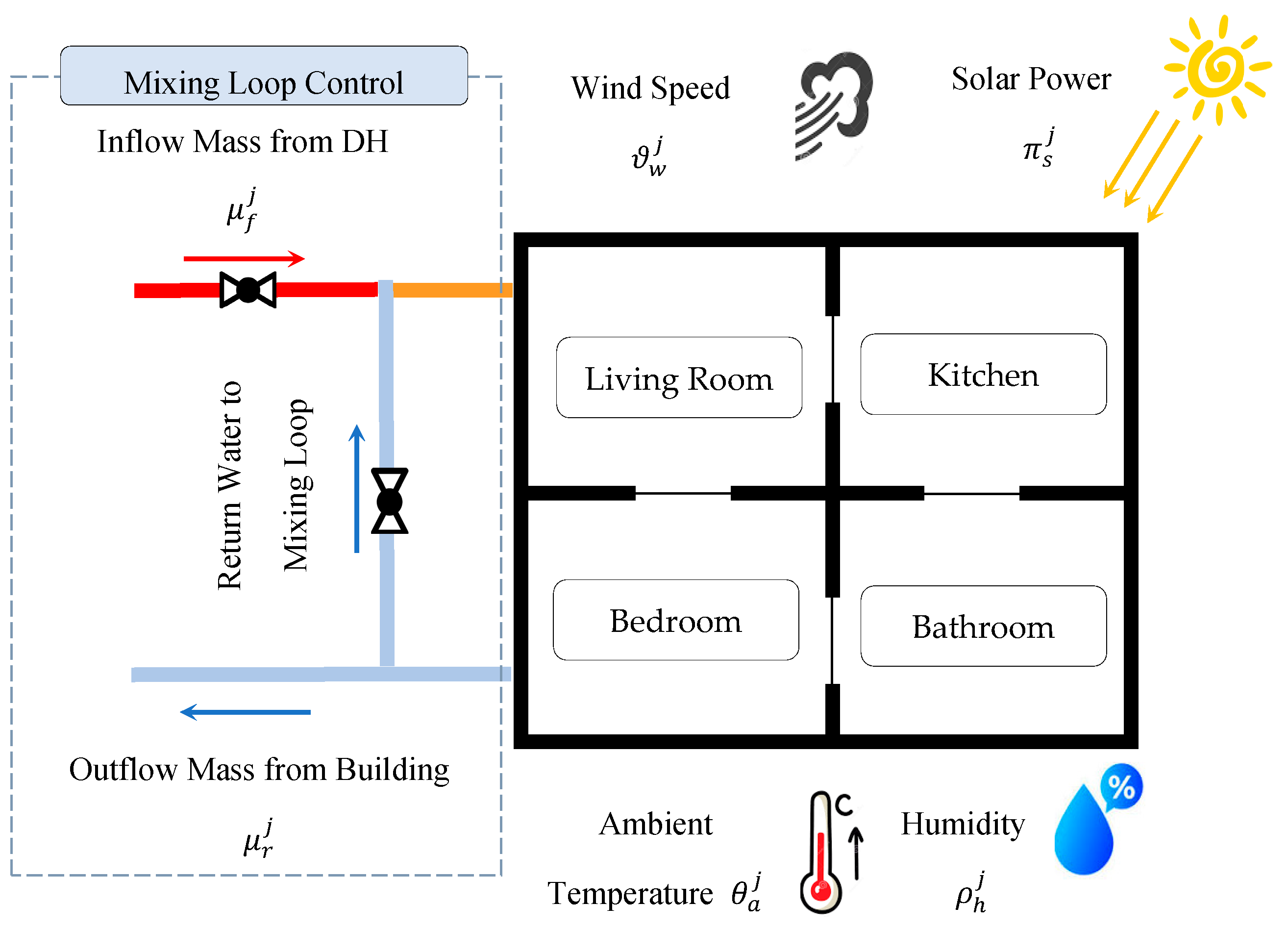
In this section, the proposed approach to forecasting the energy consumption of residential buildings is explained. The study aims to forecast the energy injected into buildings through a mixing loop of DH. The energy drawn from the mixing loop is used for space heating and DHW consumption.

Figure 1 shows a schematic diagram of a detached house supplied by a mixing loop. As the diagram reveals, the space heating energy is mainly dependent on weather variables, e.g., ambient temperature, solar irradiation, wind speed, humidity, and residents’ behavior, e.g., comfort temperature, occupancy pattern, and heat waste of household appliances. Furthermore, the DHW consumption is normally a function of some residents’ behavior, e.g., showering, cooking/dishwashing, and laundering.

The present methodology aims to forecast the future energy consumption of buildings without needing full access to the affecting factors. Therefore, informative input data are recorded by measurement sensors to train machine-learning algorithms.

2.1. General Framework

The suggested approach is comprised of four stages as follows:

Data Measurement by the Installed Sensors: In the first stage, the data from the mixing loop and DH are recorded by the installed sensors for a specific period $t ϵ \left[{\tau }_i,{\tau }_{i+T}\right]$. Let us assume the HSP supplies $j ϵ \left[1,J\right]$ residential buildings. The measured data are classified into weather and energy data. The weather data includes ambient temperature ${\theta }_a^j\in ℝ$, solar irradiation ${\pi }_s^j\in ℝ$, wind speed ${\vartheta }_w^j\in ℝ$, and humidity ${\rho }_h^j\in ℝ$. The energy data comprises forward water temperature ${\theta }_f^j\in ℝ$, return water temperature ${\theta }_r^j\in ℝ$, forward mass flow ${\mu }_f^j\in ℝ$, and return mass flow ${\mu }_r^j\in ℝ$. Therefore, the complete set of measured data can be stated as follows:

$$\mathsf{\Psi }=\left\{{\theta }_a^j(t),{\pi }_s^j(t),{\nu }_w^j(t),{\rho }_h^j(t),{\theta }_f^j(t),{\theta }_r^j(t),{\mu }_f^j(t),{\mu }_r^j(t),\forall t\in \left[{\tau }_i,{\tau }_{i+T}\right]\&j\in \left[1,J\right]\right\}$$

(1)

Data Priority Sorting: In this stage, the sensor data are sorted to find the top priorities. It means that the sensor data are evaluated to find the most informative variables affecting the energy consumption of the buildings. Regarding the weather data, the PCA is run to find the most effective variables. In the case of energy data, the lowest variables are measured to calculate the energy consumption of the buildings. Therefore, no data dimension reduction is conducted on the energy data. The reduced set of measured data are formulated as follows:

$$\overline{\mathsf{\Psi }}=\left\{{\overline{\Pi }}_{j,t}^W,{\overline{\Pi }}_{j,t}^E,\forall t\in \left[{\tau }_i,{\tau }_{i+T}\right]\&j\in \left[1,J\right]\right\}$$

(2)

where ${\overline{\Pi }}_{j,t}^W$ and ${\overline{\Pi }}_{j,t}^E$ are the reduced set of weather and energy data, respectively. Note that the mathematical equation to calculate the energy consumption of the buildings using the sensor data is expressed as follows:

$${\pi }_h^j(t)={\eta }_{water}\times {\mu }_f^{*j}(t)\left({\theta }_f^{*j}(t)-{\theta }_r^{*j}(t+{\tau }_{cycle})\right)$$

(3)

where ${\pi }_h^j\in ℝ$ is the heat consumption of the building, ${\eta }_{water}$ is the specific heat capacity of the heat carrier, i.e., water. Note that the asterisk symbols for the mass flow and temperature denote the data values after the mixing loop. Meanwhile, due to the heat carrier circulation in the buildings, the return temperature is measured with ${\tau }_{cycle}$ delay time. The parameter shows the time the heat carrier takes to complete one cycle in the heating pipes of the building. At the end of this stage, the primary data set $\mathsf{\Psi }$ is transformed into the reduced data set $\overline{\mathsf{\Psi }}$ with lower and informative data.

Energy Model Estimation: In this stage, the set of reduced data $\overline{\mathsf{\Psi }}$ is processed by machine-learning algorithms to build a mapping function for the energy consumption of the buildings. The mapping function estimates the energy consumption model of the building, i.e., ${\overline{\Pi }}_{j,t}^E$, in response to the reduced weather data ${\overline{\Pi }}_{j,t}^W$. The estimation model is expressed as follows:

$${\pi }_h^{j,e}(t)=\begin{array}{cc}f\left({\overline{\Pi }}_{j,t}^E{|}_{{\overline{\Pi }}_{j,t}^W}\right)+{\epsilon }_{error}^e& ,\forall t\in \left[{\tau }_i,{\tau }_{i+T}\right]\&j\in \left[1,J\right]\end{array}$$

(4)

where f denotes the estimation function applied by machine-learning algorithms and ${\epsilon }_{error}^e$ is the estimation error between the measured ${\pi }_h^j$ and estimated energy ${\pi }_h^{j,e}$. In this study, three algorithms, including ANN, k-nearest neighbors (k-NN), and linear regression model (LRM), are addressed. Note that the mapping function is built for the training data period.

Future Energy Forecasting: In this stage, the estimation function f is used to forecast the energy consumption of the buildings in the future, i.e., $t ϵ \left[{\tau }_{i+T},{\tau }_{i+T+F}\right]$, in response to weather data forecasting. Note that T and F are the duration of training and forecasting periods, respectively. Therefore, they are formulated as follows:

$${\pi }_h^{j,f}(t)=\begin{array}{cc}f\left({\overline{\Pi }}_{j,t}^W\right)+{\epsilon }_{error}^f,& \forall t\in \left[{\tau }_{i+T},{\tau }_{i+T+F}\right]\&j\in \left[1,J\right]\end{array}$$

(5)

where ${\epsilon }_{error}^f$ describes the forecasting error.

Uncertainty Characterization: In this stage, uncertain scenarios are generated for future weather data. In order to forecast the energy consumption of the buildings in the previous stage, the future weather data are forecasted. Therefore, deterministic weather data may fail in real applications. To make the approach compatible with the real world, scenario generation schemes are addressed to incorporate plausible weather uncertainties into the forecasted weather data. In this way, two approaches, including stochastic scenarios [23] and envelope bounds [24], are suggested as follows:

$${\overline{\Pi }}_{j,t}^{W,U}={\overline{\Pi }}_{j,t}^W+{\omega }_{j,t}^{\kappa }$$

(6)

$${\omega }_{t,j}^{\kappa }=\left\{\begin{array}{cc}t\in \left[{\tau }_{i+T},{\tau }_{i+T+F}\right]\&j\in \left[1,J\right],& \forall ({\omega }_{j,t}^{\kappa },p_{j,t}^{\kappa })\in f_{pdf}(.)\\ \forall \kappa =1,\dots ,K_{\omega }:& {\displaystyle \sum _{k=1}^{K_{\omega }}{p}_{j,t}^k=1}\end{array}\right\}$$

(7)

$${\omega }_{t,j}^{\kappa }=\left\{\begin{array}{cc}t\in \left[{\tau }_{i+T},{\tau }_{i+T+F}\right]\&j\in \left[1,J\right],& \forall {\omega }_{t,j}^{\kappa }\in \left[\alpha ,\alpha +{\delta }^{\kappa }\right]\\ \forall \kappa =1,\dots ,K_{\omega }:& {\delta }^{\kappa }=\kappa \times \frac{\left|\alpha -\beta \right|}{K_{\omega }}\end{array}\right\}$$

(8)

Equation (6) describes that the uncertain weather data ${\overline{\Pi }}_{j,t}^{W,U}$ is the summation of the deterministic weather forecast ${\overline{\Pi }}_{j,t}^W$ and weather scenario ${\omega }_{j,t}^{\kappa },\kappa =1,\dots ,K_{\omega }$. In Equation (7), the stochastic weather scenarios are generated using different probability distribution functions, (PDF), e.g., Normal and Weibull. Each scenario has an associated probability $p_{j,t}^{\kappa }$ in which the summation of all probabilities for each time slot is equal to 1. In the second scheme, an uncertain envelope is defined with upper and lower thresholds denoted by α and β, respectively. The whole envelope is portioned into κ subintervals. Then, each subinterval shows the uncertain weather envelope. The former scheme evaluates the stochastic weather uncertainties on energy forecasting. Adversely, the latter investigates the impact of uniform weather uncertainty, in the forms of underestimation and overestimation, on energy forecasting.

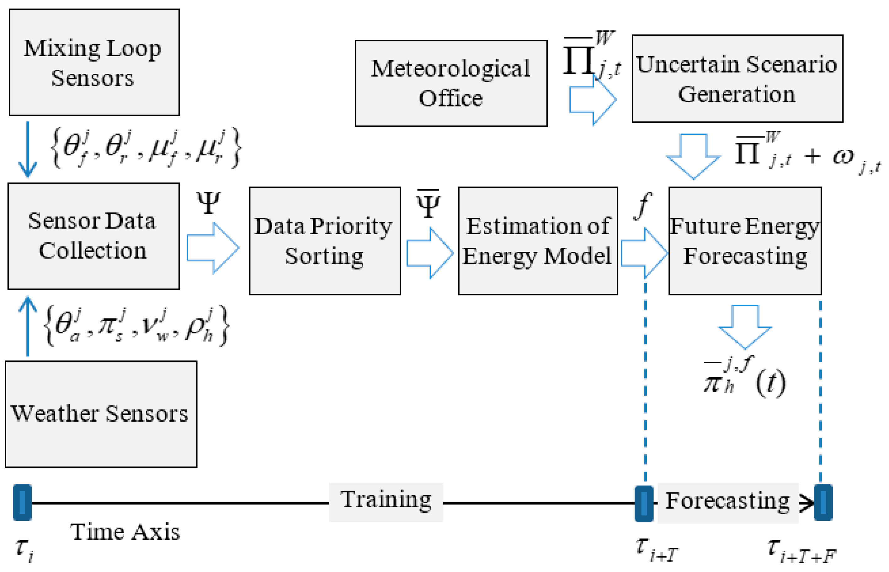
Figure 2 provides a general overview of the suggested framework from measuring sensor data to forecasting heat consumption.

2.2. Data Priority Sorting

This section aims to find the key weather data that affect the energy forecasting of residential buildings. Generally, the more data available, the more accurate the forecasting approach will be. The share of some weather data on energy forecasting is relatively low. Therefore, some weather parameters increase the computational burden of the forecasting approach, while the impact on the forecasting accuracy is relatively low. To find the most significant weather parameters, a backward elimination based on PCA is addressed [25]. This approach sorts all the weather variables based on the information they contain. The weather data correspond to small eigenvalues, which have less impact on the heat consumption of the buildings. If such variables are removed from the forecasting approaches, little information will be lost. Therefore, the key weather data with high eigenvalues are selected not only to lower the computational burden of the forecasting approaches but also to decrease the need for sensor installations and measurement. The hybrid PCA + Backward Elimination takes the following actions:

Step (1) Collect all the sensor weather data plus the energy consumption of the building j, calculated by Equation (3), and form matrix Γ with T + 1 rows and z + 1 columns as follows:

$${\Gamma }_{(1)}^j={\left[\begin{array}{ccccc}{\pi }_h^j({\tau }_i)& {\theta }_a^j({\tau }_i)& {\pi }_s^j({\tau }_i)& {\nu }_w^j({\tau }_i)& {\rho }_h^j({\tau }_i)\\ {\pi }_h^j({\tau }_{i+1})& {\theta }_a^j({\tau }_{i+1})& {\pi }_s^j({\tau }_{i+1})& {\nu }_w^j({\tau }_{i+1})& {\rho }_h^j({\tau }_{i+1})\\ .& .& .& .& .\\ .& .& .& .& .\\ {\pi }_h^j({\tau }_{i+T})& {\theta }_a^j({\tau }_{i+T})& {\pi }_s^j({\tau }_{i+T})& {\nu }_w^j({\tau }_{i+T})& {\rho }_h^j({\tau }_{i+T})\end{array}\right]}_{\left(T+1\right)\times \left(z+1\right)}$$

(9)

Note that z is the number of weather sensor data.

Step (2) Calculate the mean of all columns, $mean\left({\Gamma }^j\right),$ and deduce from the corresponding columns (I is the unit matrix):

$${\Gamma }_{(2)}^j={\left[{\Gamma }_{(1)}^j\right]}_{\left(T+1\right)\times \left(z+1\right)}-{\left[I\right]}_{\left(T+1\right)\times 1}\times mean{\left({\Gamma }^j\right)}_{1\times \left(z+1\right)}$$

(10)

Step (3) Form the covariance matrix:

$${\Gamma }_{(3)}^j={\left[Cov({\Gamma }_{(2)}^j)\right]}_{(z+1)\times (z+1)}$$

(11)

Step (4) Calculate the eigenvalues ${\Gamma }_{\left(4\right)}^{j,EValue}$.

Step (5) Sum the diagonal arrays of ${\Gamma }_{\left(4\right)}^{j,EValue}$ (scalar value):

$${\Gamma }_{(5)}^j=SumDiag({\Gamma }_{(4)}^{j,EValue})$$

(12)

Step (6) For z = 1:Z, remove column z and replicate steps 2 to 5.

Step (7) Calculate the difference between the scalar value of ${\Gamma }_{\left(5\right)}^j$ for primary and reduced ${\Gamma }_{\left(1\right)}^j$ as follows:

$${\Gamma }_{(6)}^j={\Gamma }_{(5)}^j-{\Gamma }_{(5)}^{j,Reduced}$$

(13)

Step (8) Form a matrix whose first column is ${\Gamma }_{\left(6\right)}^j$ in descending order, and the second column is the associated weather variable z. The highest z weather data show the highest PCA rank. Note that to make the ${\Gamma }_{\left(6\right)}^j$ values comparable, the weather data are normalized based on the maximum value in the measurement period.

2.3. Energy Model Forecasting

This section aims to forecast the heat energy consumption of the buildings using the processed data in Section 2.1 and Section 2.2 To achieve this aim, three machine-learning algorithms, including ANN, LRM, and k-NN, are addressed.

(1) Artificial Neural Network (ANN): the ANN is a fast, efficient and practical software tool to forecast the future demand of power systems [26], renewable power generation [27], and heat demand of residential buildings. In this study, a multi-layer perceptron (MLP) is used to train the forecasting engine with historical weather and energy variables as input data. The MLP forecasts the energy consumption of the buildings for future time slots in response to stochastic/uncertain estimation of future weather conditions. The ANN is trained and simulated in MATLAB software.

(2) Linear Regression Model (LRM): The LRM is a simple method to find a linear relationship between the input and outputs of a system. In this study, the LRM aims to forecast the future heat consumption of the buildings in response to the weather data. The LRM is trained by the historical energy consumption of the households in R software.

(3) K-Nearest Neighbors (k-NN): The k-NN is a classic, simple, and efficient forecasting method. This method observes the measured data and finds the k-nearest neighbors for future estimation [28]. The forecast values are calculated based on the average of the k-nearest neighbors. In this study, the approach investigates the similarity between the weather variables of historical data and future forecasts. Detecting the nearest neighbors, the future heat consumptions are calculated based on the weighted average of the k-nearest neighbors.

2.4. Error Criteria

In this stage, the mathematical formulations of error criteria are stated. The error indices convey the accuracy of the forecasting approaches. To make the approach comparable with other studies, the error indices are described in terms of energy unit (kW) and percentage (%). The former gives the HSP a general insight into the forecasting accuracy concerning the nominal energy consumption. The latter makes it comparable with the forecasting accuracy of other studies. Then, the error criteria are described as follows:

$$\mathrm{MAE}=\frac{{\displaystyle \sum _{i=1}^N\left|{\pi }_{h,i}^{j,f}-{\pi }_{h,i}^j\right|}}{N}$$

(14)

$$\mathrm{NMBE}=\frac{{\displaystyle \sum _{i=1}^N{\pi }_{h,i}^{j,f}-{\pi }_{h,i}^j}}{N\times \overline{{\pi }_{h,i}^j}}$$

(15)

$$\mathrm{MAPE}=\frac{1}{N}\times {\displaystyle \sum _{i=1}^N\left|\frac{{\pi }_{h,i}^{j,f}-{\pi }_{h,i}^j}{{\pi }_{h,i}^j}\right|}$$

(16)

$$\mathrm{MBE}=\frac{{\displaystyle \sum _{i=1}^N{\pi }_{h,i}^{j,f}-{\pi }_{h,i}^j}}{N}$$

(17)

$$\mathrm{CVRMSE}=\frac{1}{\overline{{\pi }_{h,i}^j}}\times \sqrt{\frac{{\displaystyle \sum _{i=1}^N{\left({\pi }_{h,i}^{j,f}-{\pi }_{h,i}^j\right)}^2}}{N}}$$

(18)

where MAE, NMBE, MBE, and CVRMSE stand for mean absolute error, normalized mean bias error, mean bias error, and coefficient of variation of the root mean squared error, respectively; ${\pi }_h^{j,f}$ and ${\pi }_h^j$ are forecasted and measured energy data; $\overline{{\pi }_{h,i}^j}$ is the mean of measurement data; and N is the number of measurement data.

3. Numerical Studies

To examine the proficiency of the suggested approaches, real sensor data are used. The sensor data include (1) weather data, i.e., ambient temperature, solar irradiation, wind speed, and humidity, (2) mixing loop data including inflow/outflow temperature and mass flow. Five months’ worth of data from 1 November 2020 to 31 March 2021 is used. Among them, the first three months are used for training, and the next two months are addressed for forecasting. The data correspond to real sensor measurements from Aalborg Living Lab (ALL) in Aalborg, Denmark. The suggested approaches are coded in MATLAB R2019 software and R language using computation hardware with a 2 GHz Intel processor and 16 GB RAM.

First, the PCA is run to determine the most informative weather data. The results of the PCA analysis are stated in

Table 2. PCA ranks for 4 weather variables.

Weather Variable	Difference of Eigenvalues ${\mathbf{\Gamma }}_{\left(6\right)}^{\mathit{j}}$	Normalized Impact Factor (%)	PCA Rank
Outdoor Temperature	0.0593	40.67	1
Solar Irradiation	0.0427	29.28	2
Wind Speed	0.0388	26.61	3
Humidity	0.0050	3.44	4

. As the table reveals, the ambient temperature, solar irradiation, wind speed, and humidity are the most informative weather variables in descending order. Among them, temperature and solar power are the highest priority, with around 40.67% and 29.28% impact factors, respectively. It means that if these two weather variables are eliminated from the sensor data, a major part of important data will be lost. Therefore, the two variables are selected as informative weather data to forecast the heat consumption of the buildings.

It is worth mentioning that other weather variables may affect the energy consumption of buildings. These data may include cloud cover and snowfall [29].

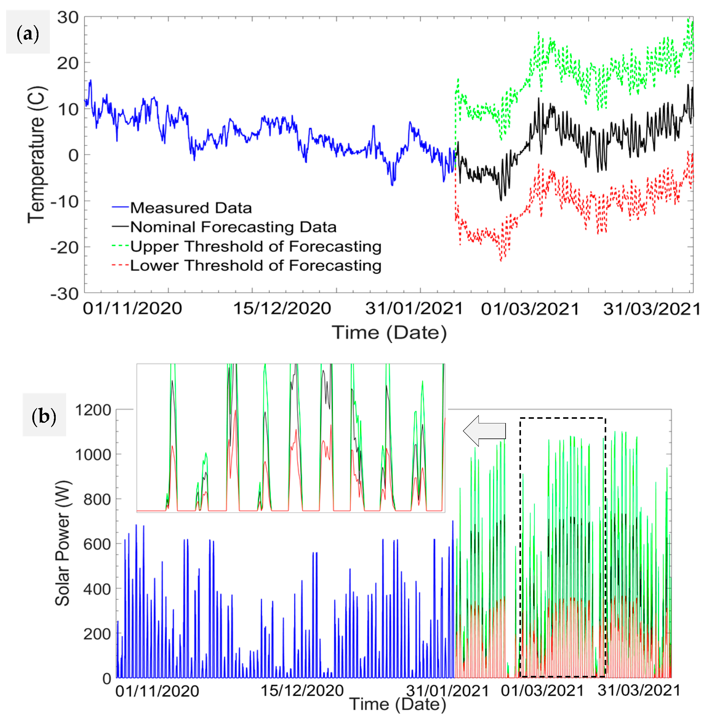
Figure 3 describes the weather data, including ambient temperature and solar irradiation, for the 5 months’ study horizon. In the forecasting period, the upper and lower forecasting thresholds are depicted in addition to the nominal forecasting.

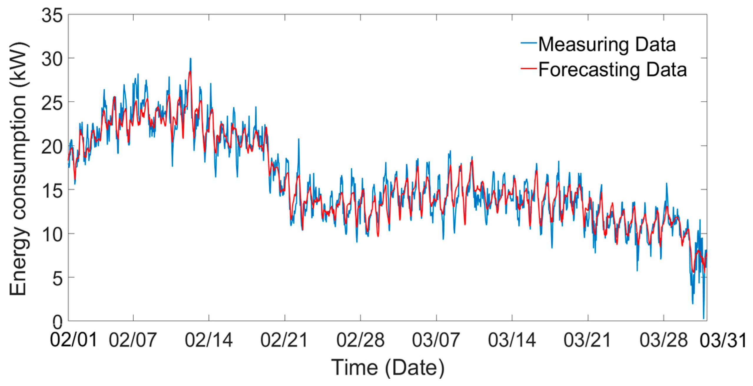
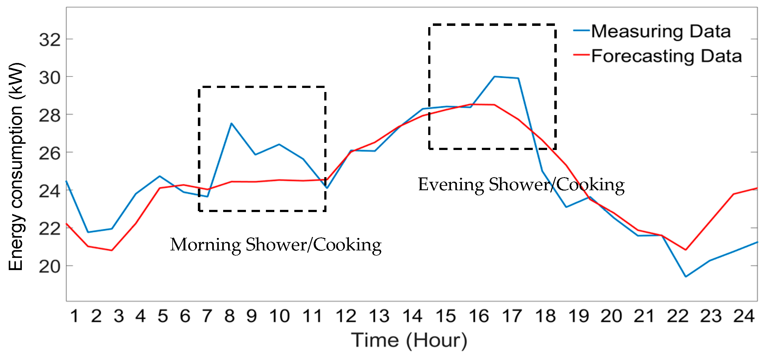
Figure 4 describes the forecasting of building heat consumption in response to the nominal informative weather data, i.e., ambient temperature and solar power, from 1 February to 31 March 2021, using the ANN. Based on the graph, the ANN estimates the heat consumption reasonably well. For this reason, the forecasting method tracks the main trend of heat consumption with high accuracy. In contrast, there are some peak periods in the daily heat profile with increased gaps between the measured and forecasted data. To elaborate on the gaps, Figure 5 depicts one-day heat consumption of the building. As can be seen, the heat profile experiences two peak periods, including hours 7–11 and 16–18. The peak periods convey the peaks of DHW for morning and evening showers. The reason is that the suggested approach forecasts heat consumption in response to ambient temperature and solar irradiation. Therefore, the occupancy patterns and DHW data are not available to be captured by the algorithm. Generally, many residents are reluctant to reveal the private data associated with their occupancy patterns. For this reason, energy meter sensors for DHW and occupancy patterns are not installed in most living labs. It shows the importance of the suggested approach to investigate the accuracy of the forecasting approach without needing private data of occupancy patterns.

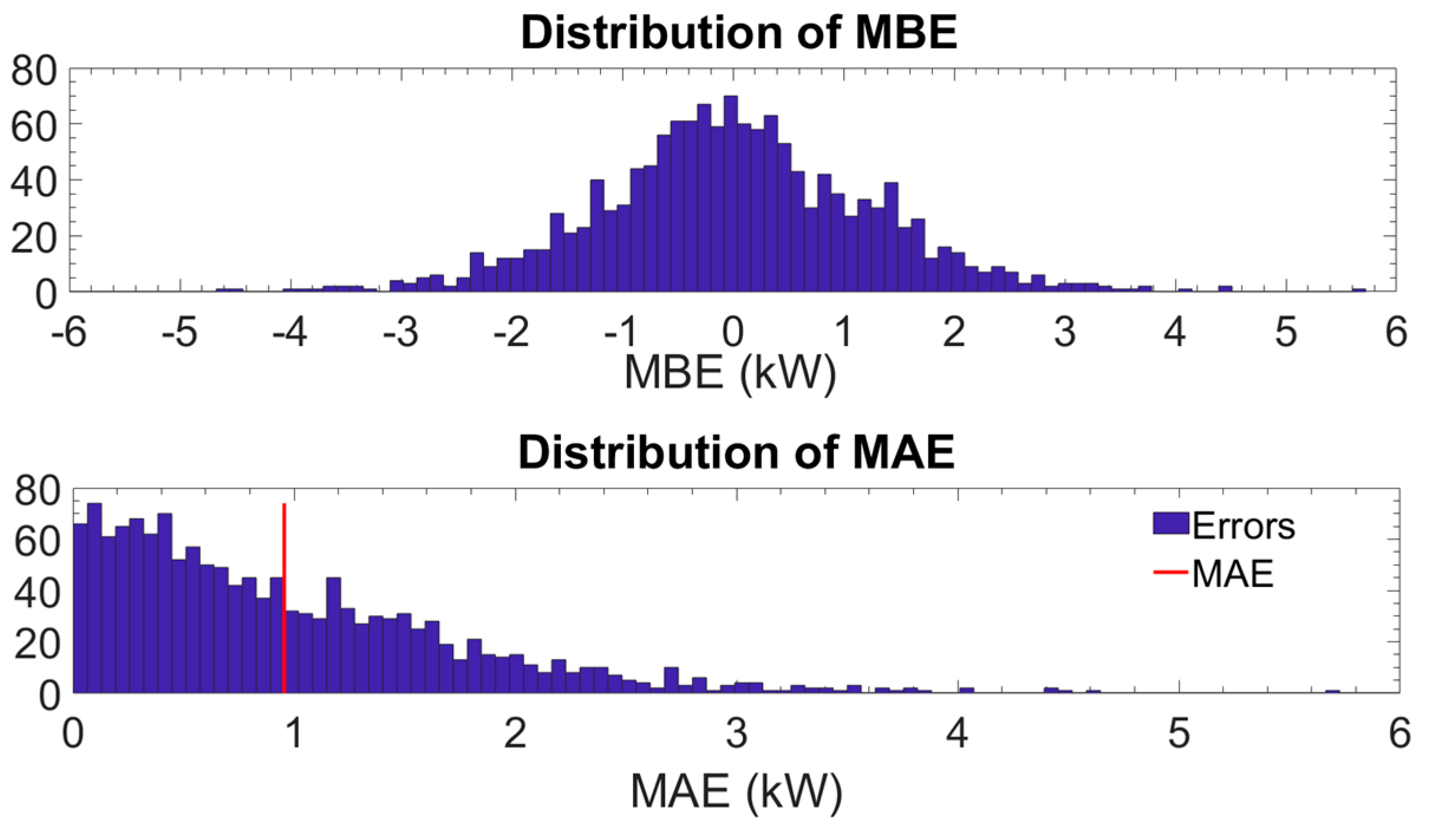
Figure 6 shows the distribution of MBE and MAE in kW during the forecasting period. The error criteria are compared with the nominal energy consumption of the building as 30 kW. Based on the bar graph, the major error is distributed in the interval [−1 + 1] kW. Besides, the average MAE is less than 1 kW.

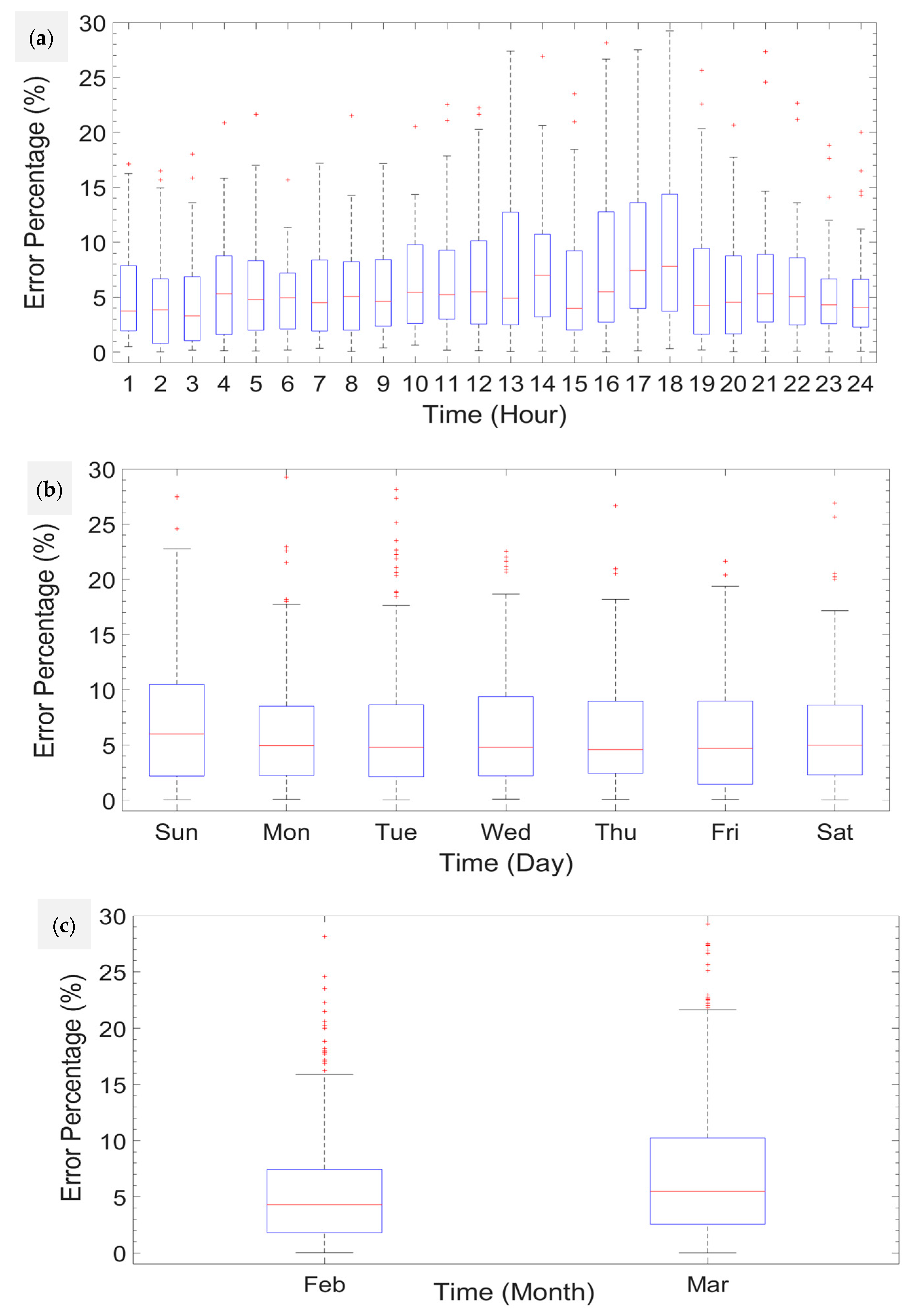
Figure 7 splits the error criteria in terms of hourly, daily, and monthly values. Regarding the hourly distribution, the highest error occurs in hours 16–18 when residents are back home after work. The immediate change of occupancy patterns has made the highest error in the forecasting approach. In contrast, the lowest hourly errors are observed in hours 2–3 and 23–24 when residents are asleep and no change is expected in the occupancy patterns.

Based on the daily distribution, Sunday encounters the highest error compared to weekdays. Following a similar pattern, the occupancy pattern at the weekend is different to that on weekdays; therefore, the forecasting approach faces lower accuracy. Meanwhile, the error percentage in March is higher than in February. One reason is that the average temperature in March is higher than in February. Therefore, the temperature in February is much closer to the temperature during the training period, i.e., from November to January.

Table 3. Comparison of error criteria for three machine-learning algorithms.

Forecasting Model	MAE (kWh)	MAPE (%)	MBE (kWh)	NMBE (%)	CVRMSE (%)
ANN	0.96	8.95	−0.00	−0.02	7.83
LRM	1.94	16.14	−0.36	−2.28	14.89
k-NN	2.12	16.36	−0.03	−0.18	16.37

compares the error criteria of the three machine-learning algorithms for the test building. In the analysis, the error parameters are calculated based on both energy and percentage units. As the table reveals, the ANN demonstrates better competence in comparison to LRM and k-NN in all criteria. Comparing LRM and k-NN, the LRM shows higher accuracy in MAE and MAPE. Therefore, the k-NN has lower residuals in MBA and NMBE criteria.

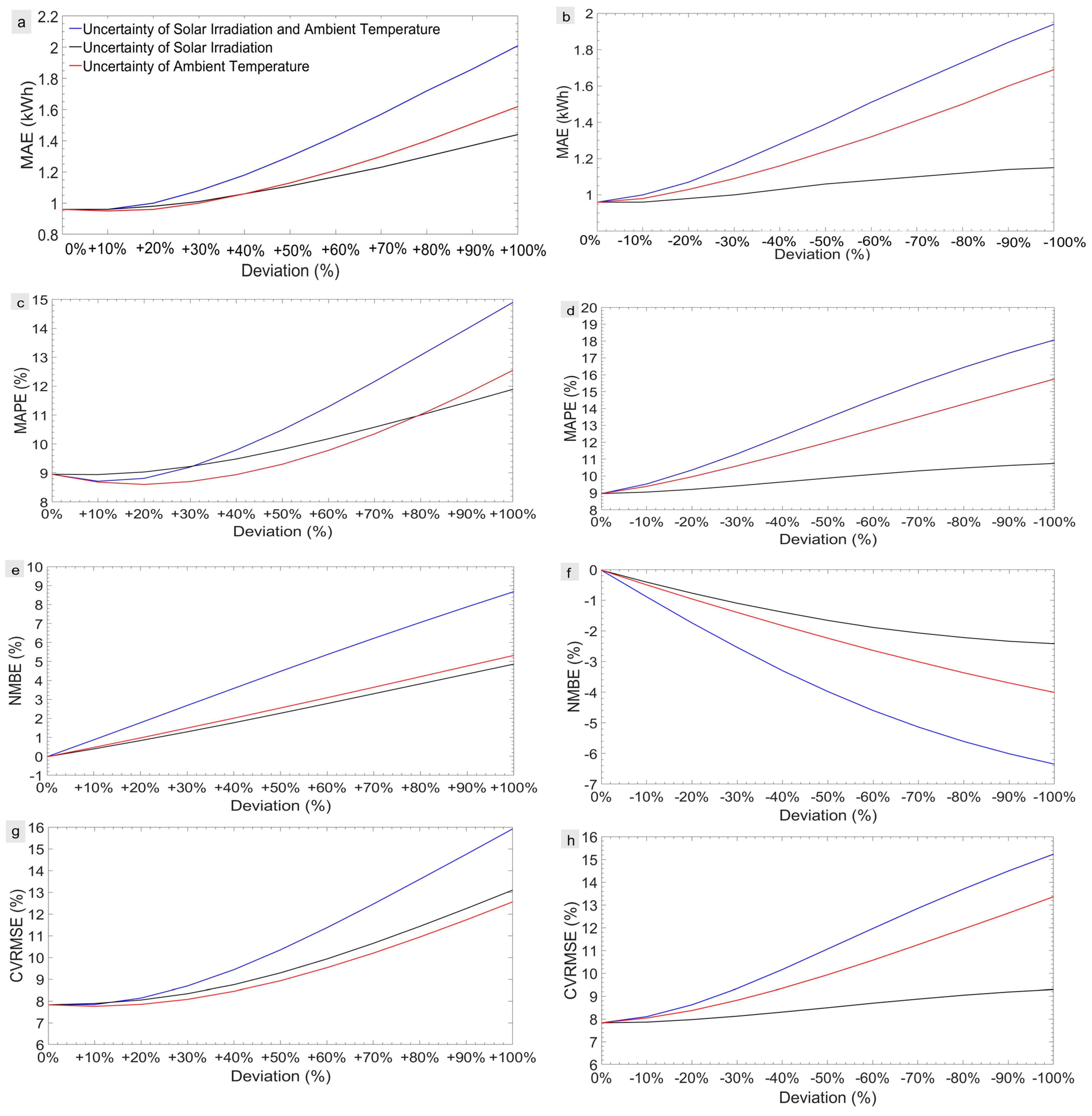
Figure 8 illustrates the impact of weather data uncertainty, i.e., ambient temperature and solar irradiation, on the error criteria. The weather uncertainties are characterized in terms of positive and negative deviation envelopes. The analysis is done for MAE, MAPE, NMBE, and CVRMSE. Based on the graphs, the following issues are observed:

1. The concurrent uncertainties of outdoor temperature and solar power pose an error in the energy estimation of up to 50% higher when compared to single weather uncertainty. For this reason, two different patterns are detected. In some error criteria, e.g., Figure 8d,f, the uncertainties of ambient temperature and solar power cause different error values. In other cases, e.g., Figure 8e,g, the error criteria of both uncertain variables are approximately the same. In both cases, the concurrent uncertainties of temperature and solar power increases the energy forecasting error considerably.

2. In most cases, the ambient temperature uncertainties have a higher impact on the accuracy of energy estimation compared to solar irradiation. This confirms the PCA results in Table 2, conveying the contributions of 40.67% and 29.28% for temperature and solar power, respectively.

3. For a specific error criterion, the negative and positive deviations follow different patterns. In MAPE, the underestimation (i.e., negative deviations) poses higher errors than the overestimation (i.e., the positive deviations). Regarding the CVRMSE, solar power shows a higher impact on the energy estimation in positive deviations. In contrast, barely any change is seen in the impact of solar power for negative deviations.

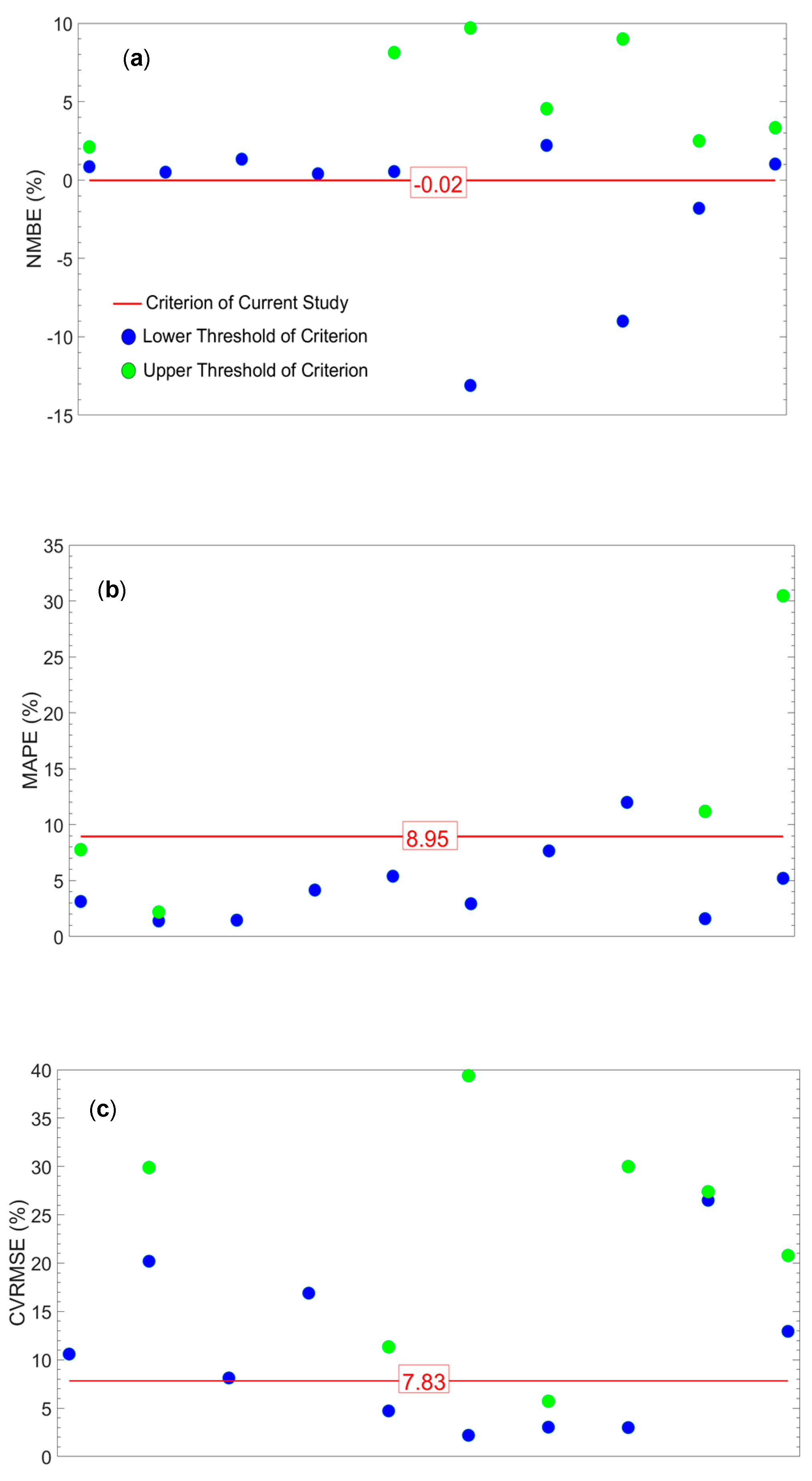
Figure 9 makes a comparison between the error criteria of the suggested approach and 10 prominent research studies between 2019 and 2022. Therefore, the percentage criteria, including NMBE, MAPE, and CVRMSE, are addressed. In some studies, upper and lower thresholds are presented for error criteria based on different forecasting methods and case studies. Regarding the NMBE, the suggested approach exhibits the best accuracy compared to the other 10 studies. For MAPE, although the other studies present better error values, the obtained criterion is within the standard level. Considering the CVRMSE, the proposed approach shows a higher accuracy than six studies out of ten.

4. Future Works

This study suggested a data-driven approach as a means of forecasting the heat consumption of residential buildings supplied by a mixing loop, using high-priority data. For the sake of energy forecasting, the HSP benefits from the following advantages:

1. Cost-effective operation of the district heating and contracted buildings to turn up/down the heat extraction when the energy price is low/high.

2. Flexible operation of the heating systems to provide demand flexibility for the upstream networks during energy shortage, or when the system reliability is jeopardized due to unforeseen failures.

3. Facilitate the integration of renewables into DH systems to decarbonize cities and suburbs.

Although the abovementioned items are the key points for HSPs, the DH plays a more critical role in future energy system structures. In countries with high renewable power penetration, like Germany and Denmark, the Power-to-X (P2X) structure makes it possible to convert, store and reconvert the surplus renewable power. In this structure, multi-carrier energy systems, e.g., power, gas, and heat, benefit from the economic, reliable, and flexible operation of the P2X. The DH and heating systems are one of the major parts of the P2X, not only to consume energy but also to provide flexibility for other P2X sectors, e.g., power-to-mobility and power-to-gas. The aim of future studies is to address the following concerns:

1. How the heat consumption of DH and aggregated buildings can be integrated into the P2X energy structure;

2. How the mixing loop controls can be coordinated to provide power flexibility for other P2X sectors, including power-to-mobility, power-to-hydrogen, etc.;

3. How large the share of DH and heating systems in the P2X structure need to be to provide a reliable, economic, and flexible operation for different sectors;

The abovementioned challenges can be addressed in future studies to investigate the contribution of DH and residential heating systems in the P2X structure.

5. Conclusions

This study suggested a practical approach to forecast the heat consumption of residential buildings supplied by a mixing loop of district heating. The approach proposed a data-driven method to extract the heating consumption using sensor data, including energy variables (i.e., inflow/outflow temperature and mass flow) and the weather data (i.e., the outdoor temperature, solar power, wind speed, and humidity). The PCA ranks and backward elimination were applied to determine the highest priority data. Finally, three machine-learning algorithms, including ANN, LRM, and k-NN, are addressed to forecast the future heat consumption of the building.

The simulation results showed that ambient temperature and solar power ranked first and second, (ahead of wind speed and humidity) with contributions to the heat consumption of 40.67% and 29.29%, respectively. Regarding the machine-learning algorithms, the ANNs showed a higher accuracy for heat consumption forecasting compared to LRM and k-NN. Therefore, the DHW consumption posed morning and evening residual peaks in the daily energy profile. In the hourly and daily error analysis, it was revealed that Sunday and the hours 16–18 on weekdays have the highest error margins due to changes in occupancy patterns. In comparison to some recent studies, the suggested approach showed high accuracy in two error criteria, including NMBE and CVRMSE.

The suggested approach can be used to estimate the flexibility potentials of residential buildings in response to renewable power intermittency. Meanwhile, it can provide cost-effective operation for HSPs considering dynamic and time-of-use energy tariffs. Although the proposed approach offers the abovementioned advantages, future studies will focus mainly on the role of residential heating systems in the P2X energy structures.