Improved Data-Driven Stochastic Subspace Identification with Autocorrelation Matrix Modal Order Estimation for Bridge Modal Parameter Extraction Using GB-SAR Data

Abstract

With the advantage of non-contact measurement, ground-based synthetic aperture radar (GB-SAR) has been widely used to obtain the dynamic deflection of various bridges. Data-driven stochastic subspace recognition (Data-SSI), a popularized time-domain technique, is commonly used for modal parameter identification of bridges. To improve the computational efficiency and accuracy of the Data-SSI method for bridge modal parameter estimation using GB-SAR, this paper proposes an improved Data-SSI method. First, boxplot data filtering is applied to screen out the error points to generate a Hankel matrix. Second, the Hankel matrix compression method is presented to reduce the ill-conditioned vectors in the column vectors of the Hankel matrix to improve calculation efficiency. Finally, the exact modal order (EMO) modal estimation algorithm based on the autocorrelation matrix is adopted to reduce the generation of false modes and improve the calculation efficiency. The results of simulation and field experiments show that the natural frequency values for the improved Data-SSI method are 2.3208 and 2.3189 and the damping ratio coefficient values are 8.10 and 8.08, under windows 1 and 2, respectively. The operation times using the improved Data-SSI method are 2.02 s and 7.61 s under windows 1 and 2, respectively. This proves that the proposed improved Data-SSI method has higher accuracy and computational efficiency.

1. Introduction

Bridge dynamic deflection is one of the most important indicators to reflect bridge structural abnormality, including the quality, operating state, and stiffness, and further provide obvious feedback on the overall deformation of bridges [1]. Compared with the traditional contact transducers, such as piezoelectric accelerometers, optical fiber sensors, strain gauges, and inductance meters, ground-based synthetic aperture radar (GB-SAR), a non-contact measurement technology, can perform all-weather, large-scale, and long-distance dynamic deflection measurement for the monitored bridges [2,3,4]. By treating the reflection points as virtual sensors, the traditional point sensors can be reduced or even eliminated [4]. Accurate comparison has been carried out between GB-SAR and accelerometers on various large bridges, which showed that the accuracy of GB-SAR was better than 0.1 mm [5,6]. With the advantages of a wide frequency response range, high sensitivity of the displacement and easy installation, GB-SAR has been widely applied in non-contact dynamic deflection monitoring of various bridges. Structural modal parameters are important indices to reflect the dynamic characteristics of the monitored bridge, which can be identified from the corresponding dynamic deflection. It is of great significance to understand the current characteristics of the monitored bridges with the determined structural modal parameters, which can provide a basis to perform state evaluation and abnormal monitoring of the bridges [7,8].

The stochastic subspace identification (SSI) method, an extension of the subspace state space system identification method, has been widely used in operational modal analysis (OMA) [8,9]. As the latest development of the time domain identification method, the SSI method can directly extract structural modal parameters from the output response signal of the structure under environmental excitation. With the characteristics of robustness, high identification accuracy, and stability, the SSI method can be used to accurately identify the frequency and damping ratio of the response signal. It has been widely used to extract modal parameters from the dynamic deflection of the monitored bridges [10,11,12,13,14,15,16,17,18]. Data-driven stochastic subspace identification (Data-SSI) and covariance-driven stochastic subspace identification (COV-SSI) are the two favorite modal parameter identification techniques [8,11]. They are all derived from the different weight matrices before the singular value decomposition (SVD). Compared with the COV-SSI method, the Data-SSI method has the ability to process a large amount of input and output data at the same time, which can ensure higher stability and accuracy. Furthermore, for the Data-SSI method, the state space matrices can be identified with robust numerical methods, such as SVD, least squares, and quadrature rectangle (QR) decomposition. Therefore, Data-SSI has been validated as one of the most robust and accurate identification methods to extract more effective information in many experiments and engineering applications [6]. George et al. proved that the Data-SSI method is accurate and effective to identify the structural abnormality in a structural abnormal monitoring experiment for simple structures with few components [9]. Dilena and Morassi performed a dynamic deflection measurement experiment for a cracked steel beam, which had a high accuracy in obtaining the crack position using Data-SSI method [7]. Boonyapinyo used the Data-SSI method to extract the modal parameters of a bridge model excited with the wind, and the results showed that the bridge coupling aerodynamic derivative extracted by the Data-SSI method was closer to the true value than the COV-SSI method [19].

However, the accuracy of Data-SSI is limited by the noise existing in monitored data. During the dynamic deflection acquisition of the monitored bridges using GB-SAR, noise and abnormal data due to environmental incentives will inevitably be generated. Moreover, modal omissions and false modalities may be caused for mode estimation using the singular value average method, due to empirical judgment for dividing the singular value inflection point of the projection matrix. In addition, the steady-state graph modal estimation method is still based on empirical judgments; it has a complicated structure and requires a large amount of calculation. Ubertini proposed a Data-SSI method to filter the error modalities for automatic modal identification of two field bridges. The results indicated that the Data-SSI method used is effective for natural frequency identification [20]. Hoofar et al. proposed an improved Data-SSI with a weight matrix to perform structural health monitoring and modal parameter identification for Alamosa Canyon Bridge; the experimental results showed that the improved Data-SSI has a high robustness [21]. However, as the Hankel matrix is directly composed of dynamic response signals, the number of columns of the Hankel matrix tends to infinity, which requires a large amount of memory, theoretically. Moreover, QR-decomposition and SVD decomposition operations increase the computational burden in the identification process greatly.

For the bridge dynamic deflection value collected by GB-SAR, it has an important impact on the collected data of the noise generated by the environmental excitation. The traditional Data-SSI method not only has a low calculation efficiency, but also contains ill-conditioned column vectors during the process of generating the Hankel matrix. They easily produce false modals and reduce the accuracy of the results. Therefore, to efficiently obtain the accurate structural modal parameters of the monitored bridge based on the dynamic deflection collected by GB-SAR, in this study, an improved Data-SSI method with autocorrelation matrix modal order estimation is proposed. In order to reduce the influence of noise and abnormal data for the dynamic deflection of the monitored bridge obtained by GB-SAR, boxplot data filtering is used to screen out the error points to generate the Hankel matrix. To reduce the ill-conditioned vectors in the column vectors of the Hankel matrix, the Hankel matrix compression method is presented to improve calculation efficiency. To reduce the generation of false modes and improve the calculation efficiency, an exact modal order (EMO) estimation algorithm based on the autocorrelation matrix is adopted.

2. Methodology

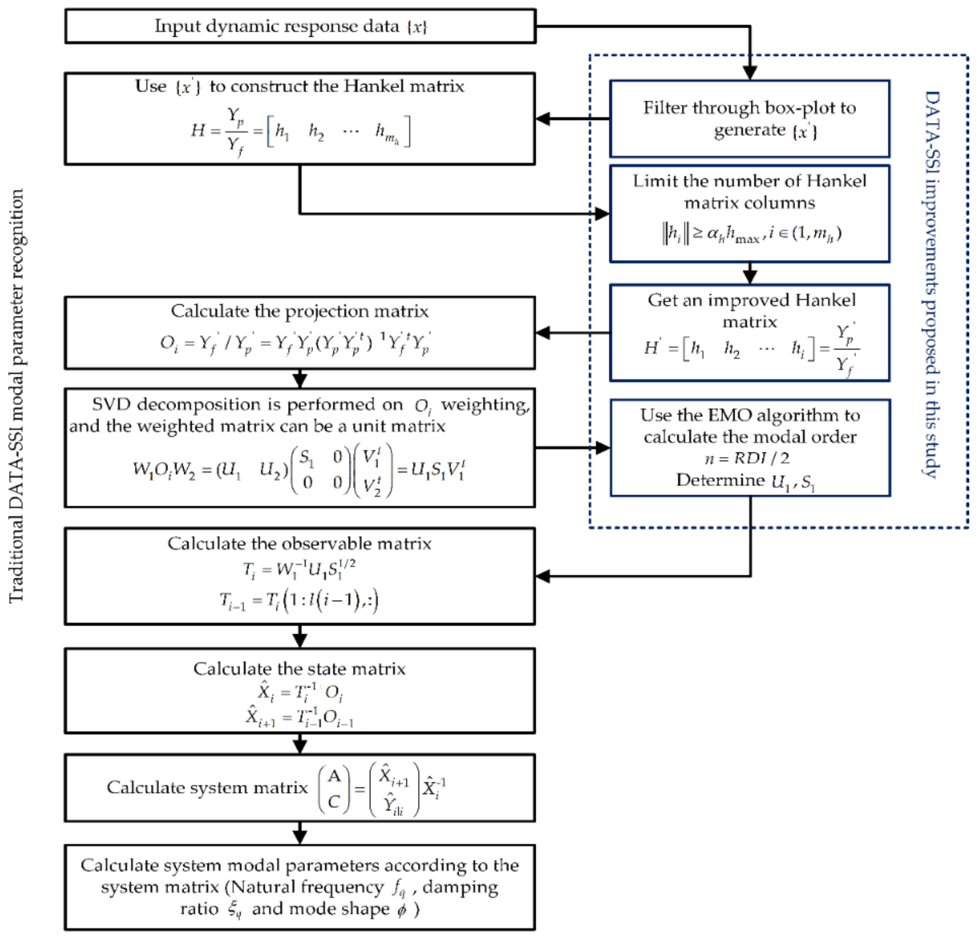
The entire workflow of the improved Data-SSI method is shown in Figure 1, which can be used to extract the accurate structural modal parameters of the bridges based on the dynamic deflection acquired by GB-SAR. It includes the following three key steps: (1) boxplot data filtering is adopted to reduce the effects of noise and abnormal data to generate the Hankel matrix, (2) the Hankel matrix compression method is presented to reduce the ill-conditioned vectors in the column vectors of the Hankel matrix, which can improve calculation efficiency, and (3) an EMO estimation algorithm based on the autocorrelation matrix is adopted to reduce the generation of false modes and improve the calculation efficiency.

More detailed Data-SSI algorithm principles and processes can be found in [10,11]. This article will not discuss them further due to space limitations.

2.1. Boxplot Data Filtering

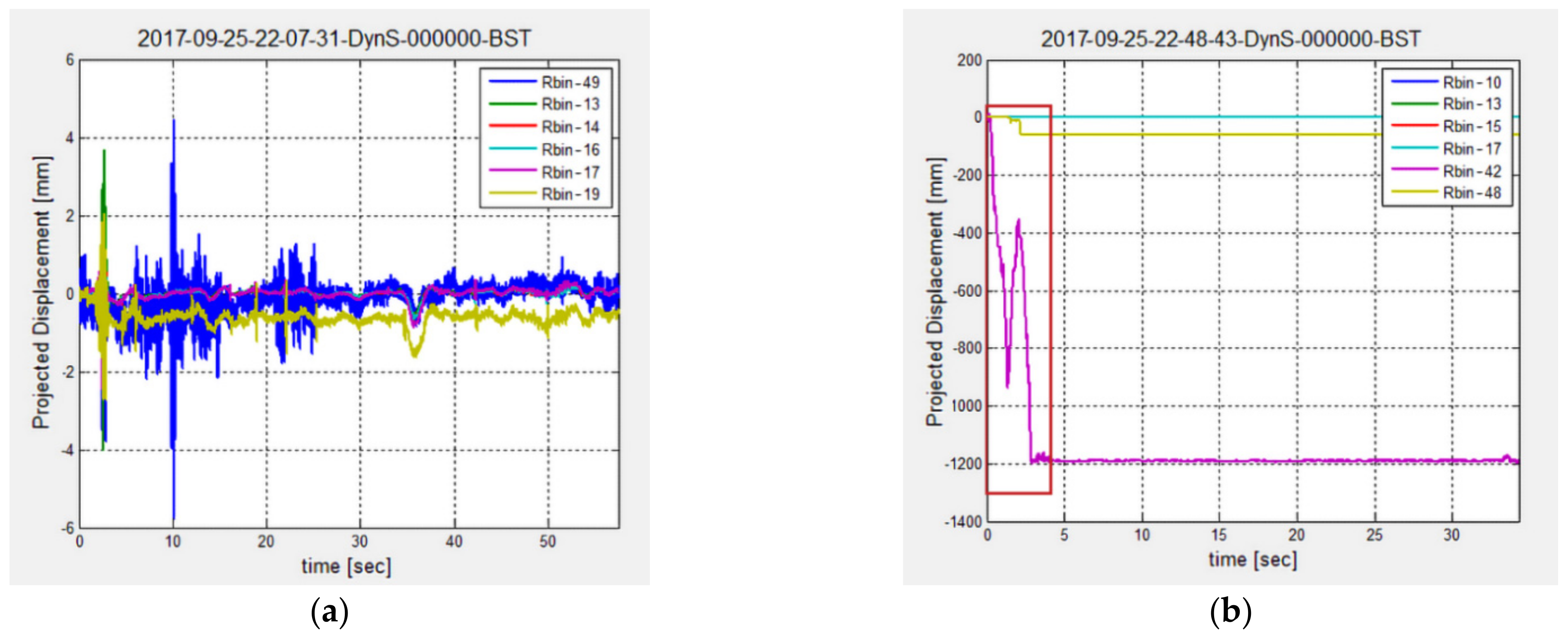
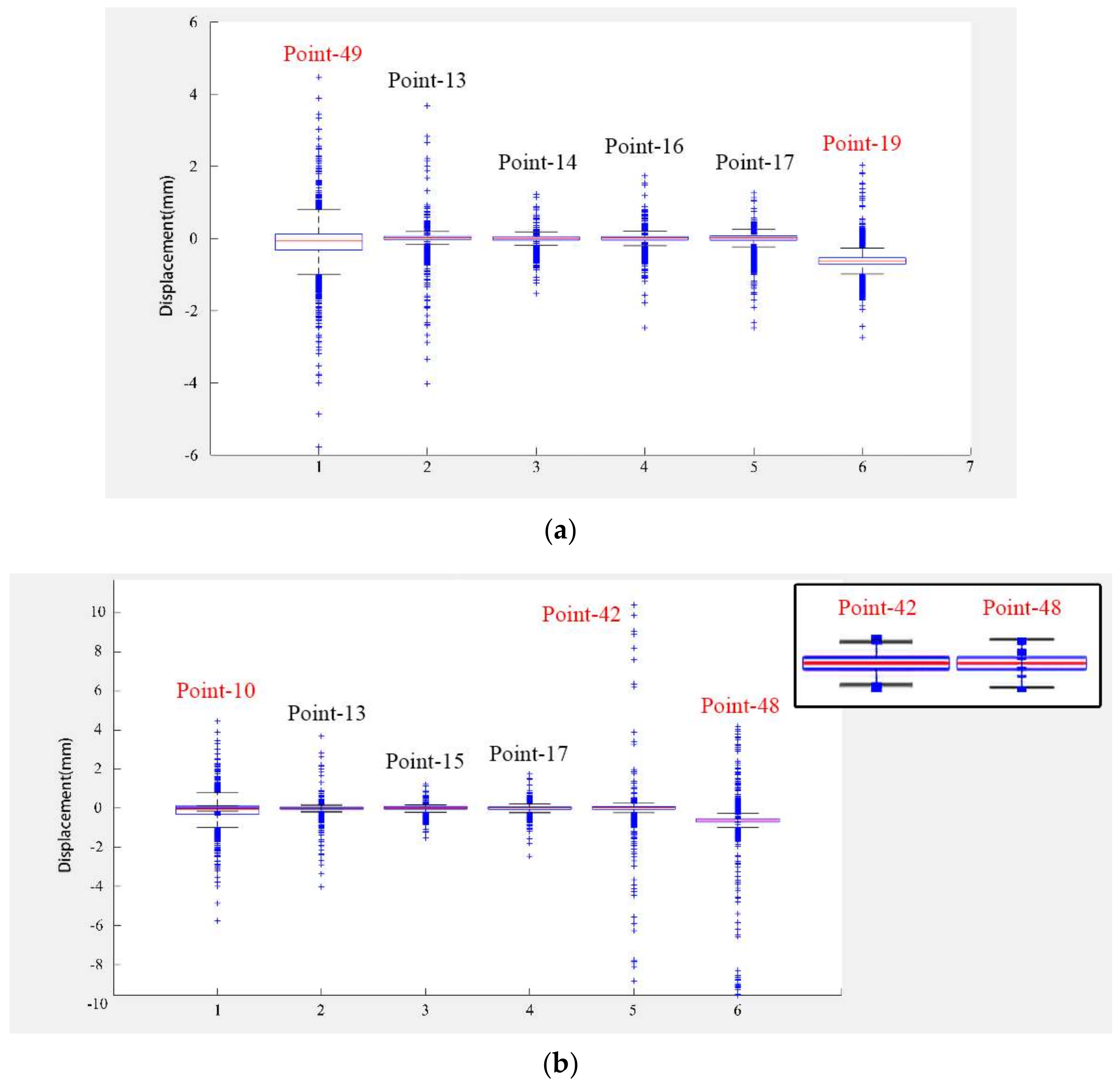
As a basic tool for visualizing the arrangement and statistical characteristics of data, a boxplot can provide univariate information for multivariate display [22]. The noise and abnormal data often are produced to pollute the obtained dynamic deflection, which are much larger (or smaller) than the vibration amplitude of the bridge itself. Therefore, in this study, boxplot filtering is performed to remove these abnormal data.

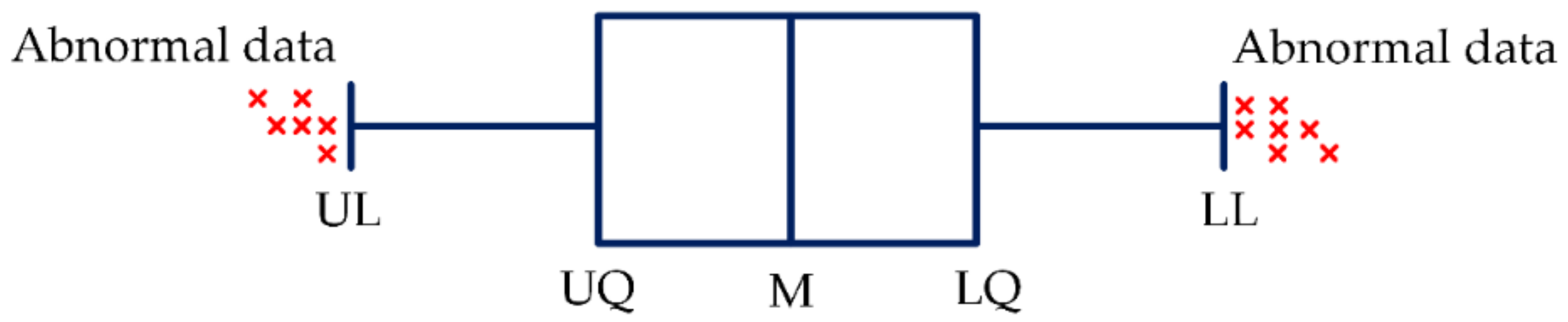
A schematic diagram of the working principle of boxplot filtering is shown in Figure 2. For a set of original signals, it needs to calculate 5 important values to build a box-plot model, including the median $M$, upper quartile $UQ$, lower quartile $LQ$, upper limit $UL$, and lower limit $LL$. In this study, the dynamic deflection is sorted in descending order in the boxplot. Therefore, $M$, $UQ$, and $LQ$ can be easily found individually. $UL$ and $LL$ are obtained by the following equations:

$$UL=UQ+k\times IQR$$

(1)

$$LL=LQ-k\times IQR$$

(2)

$$IQR=UQ-LQ$$

(3)

For the coefficient $k$ in Equations (1) and (2), Frigge et al. have explored $k$ in depth and conducted experiments with a large number of small-to-medium Gaussian samples [23]. The experiment mainly discusses the effect of $k$ being 1, 1.5, 2, and 3 on the removal efficiency of data outliers under different sample sizes. The results show that when $k=1.5$, the outer proportion of each sample is about 25%, which is more suitable for removing outliers. Although the values of k and n (sample size) both affect the outlier removal rate of the boxplot, $k=1.5$ is suitable and works well for any data size [23].

The skewness and distribution of the data can be estimated according to the positions of $LQ$, $UQ$, and $M$. Potential outliers in the input dataset can be calculated and removed directly by filtering the boxplot data. During the calculation of statistical data, due to potential outliers being considered, the boxplot has the ability to identify and resist the outliers in the data.

2.2. Hankel Matrix Compression

For the traditional Data-SSI method, the Hankel matrix is mainly constructed from the output data of structural dynamic response under environmental excitation [13]. The purpose of Hankel matrix construction is to obtain column subspace through projection. However, if some column vectors in the matrix have some small values, the subspace may lead to low-resolution projections, which will affect the identification results. In addition, theoretically, the number of columns of the Hankel matrix tends to infinity, which undoubtedly increases the computational pressure and memory consumption of the computer [24,25]. In this study, the “ill-conditioned” column vectors can be regarded as column vectors with lower specifications, which not only consumes computing memory, but may also cause invalid matrix projection. Therefore, it can compress the Hankel matrix by eliminating the “ill-conditioned” column vectors in the matrix.

Denote the denoised signal $\left\{x^{\prime }\right\}$ using boxplot filtering, and construct the Hankel matrix with Equation (4).

$$H=\left[\frac{Y_p}{Y_f}\right]=\left[\frac{\begin{array}{cccc}{x}_0& x_1& \dots & x_{j-1}\\ x_1& x_2& \dots & x_j\\ \dots & \dots & \dots & \dots \\ x_{i-1}& x_i& \dots & x_{i+j-2}\end{array}}{\begin{array}{cccc}{x}_i& x_{i+1}& \dots & x_{i+j-1}\\ x_{i+1}& x_{i+2}& \dots & x_{i+j}\\ \dots & \dots & \dots & \dots \\ x_{2i-1}& x_{2i}& \dots & x_{2i+j-2}\end{array}}\right]$$

(4)

where $H$ is the constructed Hankel matrix and $Y_p$ is the row space representing the “past” composed by the upper half of the matrix. $Y_f$ is the row space of representing the “future” composed by the lower half of the matrix. $i$ is the row and $j$ is the column of matrix $H$.

The choice of parameter $i$ depends on various factors related to the type of structure to be identified, including the length $s$ of the input signal and the sampling frequency $fs$. The choice of $i$ is related to the lowest frequency $f_1$ of the considered structural system. Assuming that there are $n_c$ or more cycles of the lowest frequency $f_1$ within the range of signal length $i$, then:

$$\frac{i}{fs}{f}_1>n_c$$

(5)

Since it contains at least one cycle, $i$ can be expressed as:

$$i\ge n_c\frac{fs}{f_1}=n_c\beta$$

(6)

$$\beta =\frac{fs}{f_1}$$

(7)

Although a larger value of $i$ can make a larger time window to ensure the algorithm is more stable, too large a value of $i$ will lead to a decrease in computational efficiency. Therefore, to extract enough information from the observable range space, the number of rows of the “future” output matrix is relatively large. According to Equation (6), the minimum value of $i$ can be determined through a complete minimum frequency cycle, but the value of $i$ in different situations needs to be judged empirically.

The Hankel matrix can be divided into $m$ column vectors according to each column, and further calculate the norm of each column vector. Define $h_{\max }$ as the largest norm. The “ill-conditioned” column vector with too low values can be deleted to limit the number of matrix column vectors using Equation (8).

$$‖h_i‖\ge {\alpha }_h{h}_{\max },i\in (1,m_h)$$

(8)

where $h_i$ represents any i-th column vector in the Hankel matrix. $a_h$ represents the compression ratio of the matrix between the range of $\left(0,1\right)$ and $h_{\max }$ represents the largest column vector in the Hankel matrix. $m_h$ represents the number of columns of the Hankel matrix.

2.3. Autocorrelation Matrix EMO Estimation Algorithm

For the EMO method, it is basically flat for the white noise power spectral density curve [26]. Since the power spectral density of the input signal can be represented with the eigenvalues of the autocorrelation matrix $\left(R_x\right)$, the connection point between the signal and the noise subspace will change significantly. This kind of change cannot be directly identified because it is impossible to define a threshold for the changed signal and the corresponding signal-to-noise ratio (SNR). Therefore, the relative difference $RD$ of continuous eigenvalues can be used to enhance the discrimination between the noise subspace and signal.

$$RD=\frac{{\lambda }_i-{\lambda }_{i-1}}{{\lambda }_{i+1}}(i=2,3,\cdots ,M-1)$$

(9)

where ${\lambda }_i$ is the i-th eigenvalue and the diagonal matrix of eigenvalues is sorted in descending order. $M$ is the number of eigenvalues and we define RDI as the row number sequence $I$ of the $RD$.

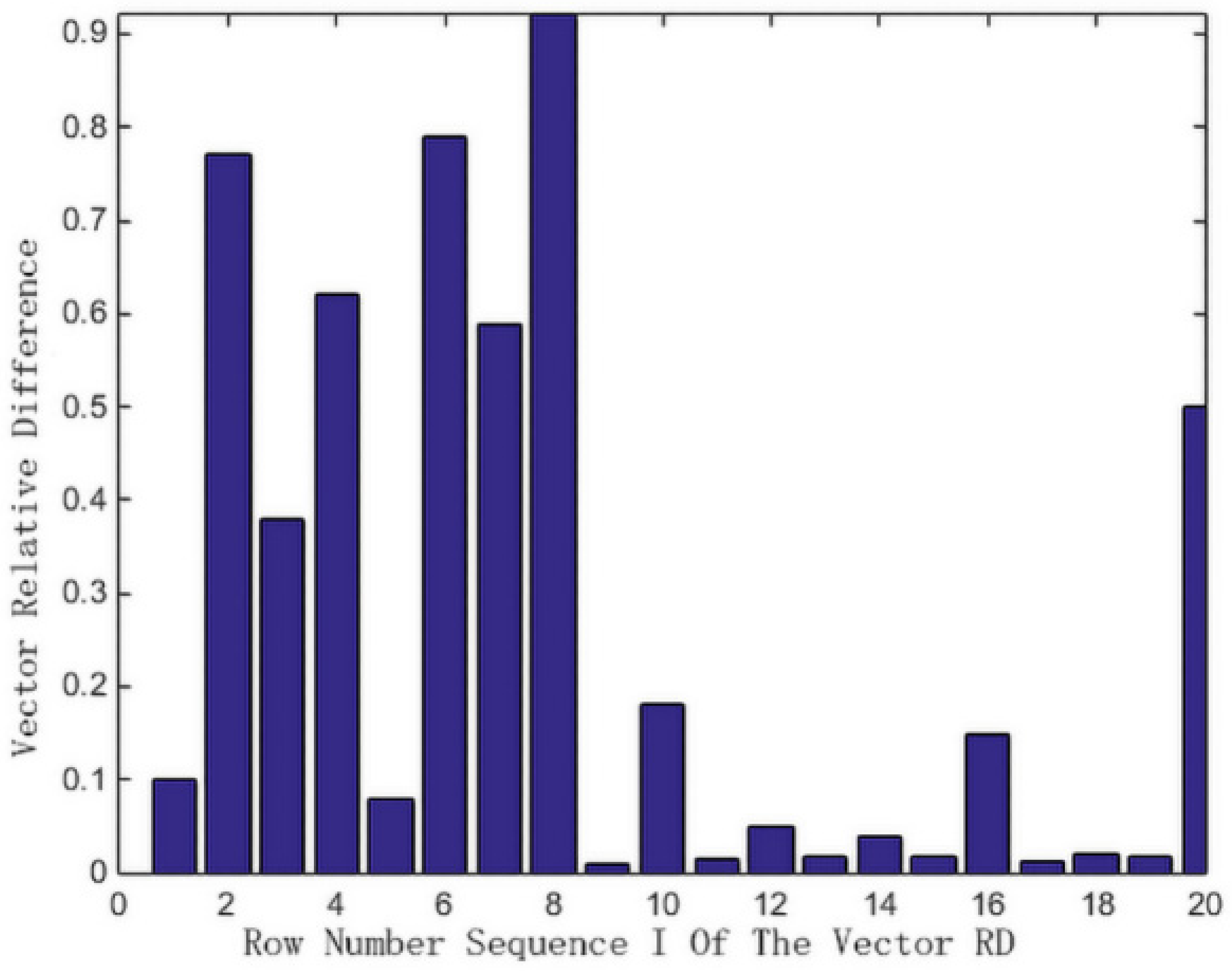
As shown in Figure 3, the peak of the relationship between RD and RDI is the potential demarcation point between the signal and noise subspace. The two consecutive eigenvalues of a special complex frequency component pair are almost equal, so the value of the odd position in the RD diagram is close to zero. Under normal circumstances, the appropriate mode order can be selected according to the RDI corresponding to the first two peaks, but when the amplitude of the harmonic component changes greatly, the selection range is extended to the five peaks to make the result more reliable.

The largest RDI is selected as the preliminary estimation of the modal, and the selected initial value is restricted to guarantee the signal component belonging to the signal subspace. The verification conditions are given as:

$${\lambda }_j\ge \beta \times \frac{{\lambda }_{j+1}+{\lambda }_{j+2}+{\lambda }_{j+3}+\cdots +{\lambda }_m}{m-j}$$

(10)

where the highest RDI value $j$ is the initial value of the mode order. $\beta$ is the sensitivity factor in the range 2–5 to determine the sensitivity of the estimated value. On the one hand, the lower the value of $\beta$, the higher the sensitivity of the estimation algorithm, which can cause overestimation, so that it can identify the small harmonic components. On the other hand, if the value of $\beta$ is high, it is likely to miss some very small order of magnitude components, leading to underestimation of the modal order. However, as for the second point, due to the low amplitude of the missing component, this has no great effect on signal reconstruction. If the algorithm fails to verify, the second highest value in the remaining peak value is used as the estimated value, and the condition judgment is performed again.

The main steps of the proposed EMO estimation algorithm are as follows:

• Construct order Hankel matrix $X$ of order based on signal $\left\{x^{\prime }\right\}$,

  $$X=\left[\begin{array}{cccc}{x}^{\prime }(0)& x^{\prime }(1)& \cdots & x^{\prime }(m-1)\\ x^{\prime }(1)& x^{\prime }(2)& \cdots & x^{\prime }(m)\\ ⋮& ⋮& \ddots & ⋮\\ x^{\prime }(n-m)& x^{\prime }(n-m+1)& \cdots & x^{\prime }(n-1)\end{array}\right]$$

  (11)
• Construct autocorrelation matrix $R_x$,

  $$R_x=\frac{X}{n-m}\times X^H$$

  (12)

  where $X$ is the Hankel matrix of order $m$, $n$ is the length of the signal $\left\{x^{\prime }\right\}$, and $X^H$ represents the Hermitian transpose of the matrix $X$;
• Carry out eigenvalue decomposition on $R_x$ and make the eigenvalue $\lambda$ in descending order;
• Calculate RD of continuous eigenvalues in descending order according to Equation (9) and draw a histogram of RD and the corresponding eigenvalue row number RDI;
• Select the maximum value of RDI corresponding to five peaks as the initial value of the modal order estimation;
• According to Equation (10), determine whether the spectral components belong to the signal subspace. If the initial modal order value satisfies the verification condition, modal order is RDI/2. Otherwise, select the next highest RDI as the new value of modal order estimation, execute step 4 in sequence until the selected RDI satisfies the verification condition.

Each mode of $R_x$ can be represented by using two main eigenvalues [27]. Therefore, the dominant eigenvalue will be twice the value of the modal order in the signal. Compared with the main eigenvalues, the remaining eigenvalues of $R_x$ are very small for the noise subspace. When the value of $i$ is twice that of the modal order, the value of RDI will rise rapidly. The reason is that ${\lambda }_i$ is a major eigenvalue belonging to signal subspace, and it is also quite low due to belonging to the noise subspace. After ${\lambda }_i$ to ${\lambda }_m$, the average value of consecutive eigenvalues is also much smaller than ${\lambda }_i$. In the EMO algorithm, this logic is used to accurately estimate the modal order.

3. Simulation Experiment

3.1. Modal Order Estimation Validation

To validate the accuracy of the autocorrelation matrix EMO estimation algorithm for modal order estimation, a simulated signal S1 was selected with known modal parameters, which has 4 frequency components. Signal S1 was used to test the strong anti-noise ability of the autocorrelation matrix EMO estimation algorithm, which was added with Gaussian noise under SNRs of 15, 20, and 25 db.

$$\begin{array}{l}S1=2\cos (2\pi \ast 0.25t+1.5\pi )·\exp (-0.17t)+2\cos (2\pi \ast 0.33t+1.5\pi )·\exp (-0.12t)\\ +2\cos (2\pi \ast 0.78t+0.5\pi )·\exp (-0.13t)+2\cos (2\pi \ast 0.87t+0.5\pi )·\exp (-0.0702t)\end{array}$$

(13)

Table 1. Comparison of modal order and modal parameters among the autocorrelation matrix EMO estimation algorithm, MP method, and ERA method.

SNR	15 dB			20 dB			25 dB
Method	Modal Order	Frequency (Hz)	AF	Modal Order	Frequency (Hz)	AF	Modal Order	Frequency (Hz)	AF
Actual value	none	0.230	0.140	none	0.230	0.140	none	0.230	0.140
		0.290	0.090		0.290	0.090		0.290	0.090
		0.460	0.110		0.460	0.110		0.460	0.110
		0.690	0.030		0.690	0.030		0.690	0.030
EMO estimation	4	0.2301	0.1410	4	0.2307	0.1400	4	0.2301	0.1410
		0.2902	0.0908		0.2900	0.0920		0.2901	0.0910
		0.4603	0.1101		0.4602	0.1100		0.4609	0.1120
		0.6900	0.0315		0.6900	0.0300		0.6902	0.0320
ERA	113	0.2304	0.1420	104	0.2311	0.1402	54	0.2497	0.1410
		0.2901	0.0990		0.2919	0.0922		0.3304	0.0920
		0.4609	0.1110		0.4604	0.1102		0.7802	0.1110
		0.6900	0.0315		0.6907	0.0308		0.6904	0.0300
MP	107	0.2300	0.1402	59	0.2300	0.1400	8	0.2298	0.1410
		0.2901	0.0918		0.2901	0.0906		0.2900	0.0910
		0.4602	0.1103		0.4600	0.1107		0.4600	0.1110
		0.6900	0.0319		0.6901	0.0301		0.6900	0.0301

shows the modal parameters of signal S1 obtained by the autocorrelation matrix EMO estimation algorithm, matrix pencil (MP) algorithm and eigen-system realization algorithm (ERA) [4,28,29,30]. The inspection of this table highlights the following. (1) As the parameterized methods for the above three methods, the accuracy of the frequency and attenuation coefficient (AF) obtained by the autocorrelation matrix EMO estimation algorithm is comparable to that of the MP method and the ERA method. (2) For the simulated signal with lower SNR, the modal order was overestimated using the MP method and the ERA method, which can cause false modes and mathematical modes. For example, for the simulated signal with SNR of 15 db, the modal order 4 can be accurately estimated using the autocorrelation matrix EMO estimation algorithm, which is consistent with the true modal order of signal S1. However, with the MP and ERA methods, modal orders were 107 and 113, respectively. Therefore, an independent algorithm is needed to filter out redundant modes. The results show that the autocorrelation matrix EMO estimation algorithm can more accurately identify the modal order of the simulated signal S1 with various SNRs, which has a stronger anti-noise performance.

3.2. Sensitivity and Efficiency Validation

To verify the sensitivity and efficiency of the improved Data-SSI method. Signal S2 was simulated to make comparison with the traditional Data-SSI method and the Fourier method, which has 3 frequency components.

$$\begin{array}{l}S2=2\cos (2\pi \ast 0.4t+1.5\pi )·\exp (-0.17t)+2\cos (2\pi \ast 0.28t+0.5\pi )·\exp (-0.05t)\\ +2\cos (2\pi \ast 0.75t+4.5\pi )·\exp (-0.13t)\end{array}$$

(14)

Table 2. Sensitivity analysis among the improved Data-SSI method, traditional Data-SSI method, and Fourier method.

SNR	15 dB				20 dB
Method	Estimated Value		Std (%)		Estimated Value		Std (%)
	F (Hz)	AF	F (Hz)	AF	F (Hz)	AF	F (Hz)	AF
Actual value	0.30	0.15			0.30	0.15
	0.35	0.03			0.35	0.03
	0.67	0.11			0.67	0.11
Improved Data-SSI	0.308	0.153	0.27	1.12	0.299	0.150	0.11	0.82
	0.350	0.033	0.05	0.40	0.349	0.030	0.04	0.25
	0.670	0.111	0.09	0.17	0.670	0.113	0.05	0.37
Traditional Data-SSI	0.310	0.151	2.27	3.71	0.301	0.153	2.14	4.11
	0.3541	0.032	2.13	3.18	0.351	0.031	2.12	4.09
	0.6701	0.112	0.06	0.19	0.679	0.112	0.05	0.39
Fourier	0.3503	0.032	0.01	0.10	0.353	0.032	0.01	0.03
	0.6701	0.111	1.37	1.08	0.674	0.116	0.55	0.43

shows the frequency and attenuation factor obtained by the Fourier method, the traditional Data- SSI method, and the improved Data-SSI method. In this study, S2 was added with Gaussian noise under the SNRs of 15 db and 20 db. The frequency and AF of S2 are identified with the average of 50 independent simulation estimations. For the Fourier method, the length and distance of the window are set to 500 and 50, respectively. For the improved Data-SSI method and the traditional Data-SSI method, the rows and columns of the Hankel matrix are set to 200 and 1000. The inspection from this table highlights the following. (1) Compared with the traditional Data-SSI, there is a great improvement for the obtained frequency and attenuation factor using the improved Data-SSI method. Especially, for the two close low-frequency parts, there is an improvement of more than 2%. The results show that the improved Data-SSI method has a better sensitivity to distinguish signals with close frequency. (2) The improved Data-SSI method can effectively identify the three different frequency parts. In this study, the 0.3 Hz mode and the 0.35 Hz mode were identified as a mixed mode by using the Fourier method. Therefore, for the modal analysis of a dense frequency system, the Fourier method cannot effectively detect all modes, especially for the modes with close frequencies in the signal, which is not suitable for short-range mode signal estimation.

Table 3. Comparison of the computation time and modal order between the improved Data-SSI method and the traditional SSI method.

Simulation Signal	SNR (dB)	Traditional Data-SSI Method			Improved Data-SSI Method
		Initial Modal Order	Final Modal Order	Calculation Time (s)	Modal Order	Calculation Time (s)
S1	15	42	4	3.21	4	1.51
	20	42	4	3.14	4	1.21
	25	42	4	3.54	4	1.26
S2	15	57	3	3.10	3	1.12
	20	60	3	3.19	3	1.16
	25	51	3	3.09	3	0.91

shows the estimated modal order and the corresponding calculation time for signals S1 and S2 with different SNRs between the improved Data-SSI method and traditional Data-SSI method. The inspection from Table 3 highlights the following. (1) For the traditional Data-SSI method, there is a problem that the initial value of the modal order is overestimated. Therefore, to obtain the accurate modal order, a separate algorithm is needed to filter out the true modals from the initial values. During the process, the modal order is changed to a higher value from the initial value. Different state matrices can be generated using these modal orders, of which the common eigenvalues represent the main modals of the signal. Therefore, although the traditional Data-SSI method can be used to obtain the accurate modal order, it requires a lot of calculation time for the establishment of state matrices and the corresponding eigenvalue decomposition. (2) Due to the accurate estimation of the modal order using the improved Data-SSI method, it is not necessary to perform refinement screening operations to reduce false modalities, which can improve the calculation efficiency. As shown in Table 3, the calculation time is less than 1.51 s for signals S1 and S2 with different SNRs, which has an efficiency improvement of more than two times. The results indicate that the improved Data-SSI method is more competitive in computational efficiency than the traditional Data-SSI method.

4. Field Experiment and Analysis

4.1. Dynamic Deflection Acquisition

The Beishatan Bridge, located in the northwest of Beijing, China, was selected as the experimental bridge in this study. Beishatan Bridge comprises the right sub-bridge (RSB) and left sub-bridge (LSB) with the same length and width, as shown in Figure 4. Since the bridge has been determined to be damaged, it is periodically monitored to ensure its operation safety. The currently known damaged area (15 m from the RSB) has a maximum deflection change of about 8 cm. The image structural interferometry (IBIS-S) instrument, a ground-based microwave interferometric radar, was used to obtain the dynamic deflection of the two sub-bridges in this experiment [4]. Without installation of multiple units on the monitored bridges, it has a higher range resolution of up to 0.5 m and a higher accuracy of up to 0.01 mm [31,32]. The measurement condition of the RSB is shown in Figure 4a. The instrument was assumed to be diagonally below the bridge, and the altitude angle of the instrument was 32°. To obtain the dynamic deflection of the same position of the LSB, the same altitude angle and distance were used as shown in Figure 4b.

The obtained dynamic deflections of the two sub-bridges are shown in Figure 5a,b. Each group contains the dynamic deflection of 6 points with the sampling frequency of 98 Hz. During the acquisition of dynamic deflection, there are many sources of interference that can generate noise and abnormal data to pollute the obtained dynamic deflection. For example, for the dynamic deflection of points Rbin 42 and 48 shown by the red rectangle in Figure 5b, they were deviated from baseline (0 mm) at the beginning caused by the passing vehicles. Therefore, it is necessary to eliminate the effects of noise and abnormal data in the dynamic deflection obtained using GB-SAR.

In order to control the influence of other environmental variables on the experiment, the duration of the whole experiment was less than 40 min. Except for the processes of sunrise and sunset, the temperature changes on the surfaces of similar structures at the same location were not significant within a time interval of 40 min. Therefore, the effect of temperature on the experiment was negligible.

4.2. Results and Analysis

Figure 6 shows the results of boxplot data filtering for dynamic deflections of Beishatan Bridge. The inspection from this figure highlights the following. (1) As shown in Figure 6a, Rbin 49 and Rbin 19 of the RSB have no valid data remaining between UL and LL after the boxplot, which is presumed to be caused by environmental impact and some other interference sources. Results on these two points are no longer discussed in later studies as no valid data are available. (2) As shown in Figure 6b, only the part with the maximum displacement less than 10 mm is shown. It can be seen more clearly from the enlarged part in the upper-right corner; although Rbin 42 and Rbin 48 still have some valid data after the boxplot, the valid data content is too low. At the same time, there was a large deviation for the sample quartiles of points Rbin 42 and Rbin 48 of the LSB, which were directly discarded in this study. One of the important reasons for the large deviation of these values is the difference in material and flatness around the reflection point. Other influencing factors such as wind, temperature, and ground vibration (vehicle passing near GB-SAR) also contribute. The results for the rest of the points indicate that the boxplot data filtering method has a good ability to reduce the influence of abnormal data.

The lowest frequency $f_{\min }$ of 2.123 Hz was obtained by Fourier transform for the original data set. The sampling frequency $fs$ of the data was 98 Hz, and the minimum value of $i$ was calculated to be 46 by Equation (6). Through a complete cycle of the lowest frequency, the minimum proportion of the “future” subspace of the Hankel matrix can be calculated as $h_{\min }=0.47$ for the required modal recognition. According to the Hankel matrix compression method described in Section 2.2, the empirical values $i=200$, $h=0.85$ were used for modal parameter estimation in this experiment.

As shown in

Table 4. Estimated modal parameters of Beishatan Bridge for the improved Data-SSI, traditional Data-SSI, and Fourier transform.

Windows	Reference Values of LSB		Improved Data-SSI		Traditional Data-SSI		Fourier Transform
	$\mathit{f}$ (Hz)	$\mathit{\zeta }$ (%)	$\mathit{f}$ (Hz)	$\mathit{\zeta }$ (%)	$\mathit{f}$ (Hz)	$\mathit{\zeta }$ (%)	$\mathit{f}$ (Hz)	$\mathit{\zeta }$ (%)
Window 1	2.318	8.3	2.3208	8.10	2.3266	7.77	2.3497	7.73
Window 2	2.318	8.3	2.3189	8.08	2.3181	7.96	2.3497	8.10

, the modal parameters of the obtained dynamic deflection for Beishatan Bridge were estimated using the improved Data-SSI, the traditional Data-SSI, and Fourier transform. Window 1 and window 2 represent the same real-time signal of the RSB in different time windows. Window 1 intercepts the signal from 20 s to 70 s for a total of 50 s, and window 2 intercepts the same signal from 20 s to 220 s for a total of 200 s. To study the modal parameters of the RSB, the experiment fits the reference values of the modal parameters through the data of the LSB, including the natural frequency $f$ of 2.318 Hz and the damping ratio coefficient $\zeta$ of 8.3%. The inspection of this table highlights the following. (1) The improved Data-SSI and the traditional Data-SSI method can correctly estimate the first-order natural frequency. The natural frequencies of the improved Data-SSI and the traditional Data-SSI method are 2.3208 Hz and 2.3266 Hz under window 1, and 2.3189 Hz and 2.3181 Hz under window 2, which are better than the results of the Fourier transform. (2) Compared with the traditional Data-SSI method and Fourier transform, the damping ratio coefficient values from the improved Data-SSI method are 8.10% and 8.08% under windows 1 and 2, respectively. They are more accurately estimated compared with the reference values.

Table 5. Operation time of the improved Data-SSI and the traditional Data-SSI methods.

Windows	Time Span	Operation Time
		Improved Data-SSI	Traditional Data-SSI
Window 1	50 s	2.02 s	10.13 s
Window 2	200 s	7.61 s	36.42 s

shows the operation time for modal parameter identification between the improved Data-SSI and traditional Data-SSI methods. Compared with the traditional Data-SSI method, the operation times are 2.02 s and 7.61 s under windows 1 and 2 using the improved Data-SSI method, respectively. It is proved that the efficiency of the proposed method has a great improvement with the help of Hankel matrix compression.

Table 6. Frequencies and damping ratios under different intensities of noise of Beishatan Bridge using the improved Data-SSI method.

SNR	15 dB		20 dB		25 dB		30 dB
Windows	$\mathit{f}$ (Hz)	$\mathit{\zeta }$ (%)	$\mathit{f}$ (Hz)	$\mathit{\zeta }$ (%)	$\mathit{f}$ (Hz)	$\mathit{\zeta }$ (%)	$\mathit{f}$ (Hz)	$\mathit{\zeta }$ (%)
Window 1	2.3204	8.03	2.3211	7.95	2.3196	8.08	2.3189	8.08
	4.6723	12.97	4.6723	12.93	4.6723	12.87	4.6723	12.91
Window 2	2.3192	8.10	2.3184	8.07	2.3185	8.13	2.3188	8.12
	4.6769	12.85	4.6769	12.91	4.6769	12.87	4.6769	12.82

shows the results of modal parameter identification of two time-windows under different intensities of noise using the improved Data-SSI method. It can be seen that the improved Data-SSI method can accurately identify the first-order and second-order natural frequencies regardless of whether it is under high- or low-SNR conditions, and the obtained damping ratio coefficient is also close to the comparison value. Therefore, compared with the traditional Data-SSI method, the improved Data-SSI method is more accurate for identifying the modal parameter of dynamic deflection under random environmental excitation.

To evaluate the safety of the Beishatan Bridge, the monitored point of the RSB with a distance of about 15 m to the IBIS-S instrument was selected to make comparison with the same position of the LSB, which is the location of the maximum deflection. Considering the vibration characteristics under the influence of different states, the first 6-order modal parameters were used as a reference. As shown in

Table 7. Modal parameters identified at distance of about 15 m.

	Frequency (Hz)			Damping Ratio (%)
Modal	LSB	RSB	Difference Ratio	LSB	RSB	Difference Ratio
1	1.597	1.895	18.7%	16.4	21.0	28%
2	3.161	2.586	18.2%	7.8	6.0	23%
3	4.75	4.112	13.4%	8.5	7.4	12.9%
4	6.336	5.876	23%	5.0	3.6	28%
5	7.96	6.918	13.1%	2.9	3.3	13.8%
6	9.588	7.912	17.5%	19.5	23	17.9%

, when taking the LSB as a completely lossless structural model, the RSB experienced a large-scale drop in frequency and an increase in damping ratio. Compared with the results of parameter identification at a distance of about 5 m, as shown in

Table 8. Modal parameters identified at distance of about 5 m.

	Frequency (Hz)			Damping Ratio (%)
Modal	LSB	RSB	Difference Ratio	LSB	RSB	Difference Ratio
1	1.587	1.568	1.9%	3.9	3.7	5.1%
2	3.170	3286	3.66%	7.6	6.9	9.2%
3	4.762	4.512	5.24%	7.8	7.61	2.4%
4	6.364	6.276	1.4%	6.1	6.2	1.6%
5	8.073	7.918	1.9%	18.5	18.1	2.16%
6	9.561	9.712	1.6%	4.5	4.4	2.2%

, it can be seen that the frequency difference and damping ratio coefficient difference for the non-damaged area are not much different from those of the lossless model. Therefore, this method can preliminarily identify the location where damage has occurred, and provide a basis for subsequent further safety assessments.

5. Conclusions

With the advantages of robustness, numerical stability, and high identification accuracy, the Data-SSI method has been successfully applied to modal parameter extraction of various civil engineering structures under operating conditions. To improve the computational efficiency and accuracy of the Data-SSI method for bridge modal parameter estimation using GB-SAR, an improved Data-SSI with autocorrelation matrix modal order estimation was proposed in this study. The results presented in this study clearly highlight the following.

• Compared with the Hankel matrix constructed directly from the original data, a box-plot filter can be used to construct a more stable Hankel matrix to improve the accuracy of the bridge dynamic deflection. The results indicate that the boxplot has a good ability to reduce the influence of the environmental noise and abnormal data.
• The small ill-conditioned column vectors can be filtered and deleted in the Hankel matrix using the improved Data-SSI method. Therefore, as the number of columns of the Hankel matrix is reduced, it not only speeds up the generation of the Hankel matrix, but also produces fewer projection errors.
• The maximum value of RDI is adopted to judge the modal order after SVD decomposition. The results of simulation and field experiments show that it has a stronger anti-noise performance and a more competitive advantage in computational efficiency than the traditional Data-SSI method.

After the natural frequency and damping ratio of the structure are accurately identified, the operating state of the bridge can be further obtained and safety assessment can be carried out by means of finite element analysis or other methods.