Abstract
Spatially variable ground motions are crucial for the seismic analysis and design of extended and multi-support structures. In this study, a new random nonstationary spatially variable ground motion model based on the propagation process of seismic waves is proposed. In particular, the amplitude and phase transfer functions of seismic waves at the local site are studied herein. The probability density function of the corresponding parameters is given. Two simple examples are used to show the generation of random ground motions. Compared with traditional methods, our proposed model not only has a clear physical background but also shows good practicability. The model should be for those researchers who want to use nonstationary spatially variable ground motions to study the seismic response of lifeline systems or building portfolios.
1. Introduction
Earthquakes are an external factor in the failure of engineering structures. In the early stage of earthquake engineering, just like the literature [1] pointed out, the earthquake motion was a wave-motion, but it was not a simple harmonic; however, recording and analyzing this wave has always been difficult. In 1933, the United States obtained the first batch of strong earthquake acceleration records in the Long Beach earthquake [2], and the study of ground motions entered a new stage.
When performing random seismic response analysis on a structure, especially when using Monte Carlo simulation methods, several random ground motion samples are often required. At present, only limited ground motion samples obtained from actual measurements at specific sites are insufficient. The problem of producing accelerations, called simulated ground motions, artificial ground motions, or synthetic ground motions, has been raised. These ground motions are not arbitrary, but the characteristics of the generated ground motions must conform to the characteristics of the specific site. The ground motions themselves need description parameters from the time and frequency domains, or domains of other signal processing technologies [3], which include peak values, duration time, and main frequency. Meanwhile, the engineering site also needs its own description parameters, such as site categories, soil shear wave velocities, epicenter distances, or some parameters of the seismic sources, corresponding to the site. The study of establishing a ground motion model is essential to establish the mapping relationship between the parameters of the ground motions and the parameters of the engineering site; thus, after the parameters of the latter are provided, the acceleration time history that meets the characteristics of the former can be obtained.
In 1947, Housner proposed the use of a random process to describe ground motions [3,4]. Since then, various researchers have proposed various ground motion simulation methods. Generally, it can be divided into three categories [5]. The first category is “source-based” methods, or physical-based methods, which are based on the physical process of the formation and propagation of seismic waves. For example, a previous study [6] proposed the establishment of a random amplitude spectrum with a seismic source, propagation path, and local site and combined the random phase spectrum to simulate random ground motions; furthermore, based on this model and combined with the ground motion database PEER NGA, Boore and Atkinson statistically analyzed the peak ground motion acceleration, peak ground velocity, and other characteristics of seismic waves and provided the prediction formula [7]. Subsequently, Boore et al. were committed to the improvement in the model and the study of model parameters [8,9,10,11]. When the seismic source is a finite fault, Motazedian and Atkinson abstracted the finite fault as a series of sub-faults, used a point-source model to simulate these sub-faults, and reflected the spectrum change of ground motions by introducing the concept of “dynamic corner frequency” [12]. The second category is the “site-based” methods, which are mainly based on the frequency spectrum characteristics or response spectrum characteristics of ground motions at the site to construct a random ground motion time history [13,14]. These methods include filtered white noise random processes, filtered Poisson processes, auto-regressive moving average model, spectral representation method, random wave theory, among others [15]. For example, Rezaeian and Kiureghian suggested a white-noise-based modulation model [16]. Vlachos et al. proposed a multimodal analytical nonstationary spectral model [15]. Liu et al. proposed a random function method for random ground motion simulation, based on the spectral representation method to reduce the problem of excessive random variables in the traditional spectral representation method [17]. The third type is a hybrid method based on the “source-based” model and the “site-based” model, and it can also be called the “semi-physical” model. This type of method not only contains certain physical parameters that can effectively reflect the physical process of earthquake propagation but also has a good reflection of the characteristics of the local site. It uses real ground motion samples in an actual ground motion database to establish a random ground motion model. Some classical semi-physical models or physical models can also refer to [5].
In addition to the simulation of ground motion at a specific point, the spatially variable ground motions within a specific engineering site have also aroused strong interest, owing to the need for seismic response analysis of lifeline engineering structures. This is a problem that we study herein. Seismic ground motions exhibit obvious differences in terms of amplitude and phase at different points in a given site. This is owing to the wave passage effect, site effect, and the effect of “pure incoherence” [18]. The change in seismic motion is the spatial variation of seismic ground motions (SVSGM). Past results have demonstrated that the SVSGM is important for the seismic analysis and design of extended structures [19,20] and multi-supported structures [21,22,23]. In some cases, the SVSGM is detrimental to the seismic design of structures [24]. Therefore, many different seismic analysis methods have been suggested to study the effect of SVSGM on structures, such as the relative motion method, large-mass method [25], displacement method [26], and multiple-support response spectrum method [27]. Meanwhile, many permanent or temporary acceleration arrays have been globally deployed to record the spatially variable ground motions. The most famous is the SMART-1 array (strong-motion array in Taiwan). It was the first large digital array of strong motions, specially designed for engineering and seismological studies of earthquakes [28] and has operated from 1980 to 1991. Furthermore, some other arrays, such as the SMART-2 array in Taiwan [29] and the Chiba Experiment Station in Tokyo, Japan [30], are also of significance.
However, using real spatially variable ground motions to realize seismic response analysis of lifeline engineering is not a good option. First, the structures were generally not distributed according to the acceleration arrays. In addition, for the stochastic seismic analysis of complex nonlinear structures, especially in the Monte Carlo simulation method, many seismic samples are required. Therefore, many random spatially variable ground motion models have been suggested to simulate the differential ground motions and are widely used in engineering practice. Generally, these models generate time histories based on a power spectral density function with a coherency function. A uniformly modulated function in the time domain is always introduced to include the temporal non-stationarities. Finally, the modulated time histories were iteratively modified to ensure that the samples were compatible with the prescribed response spectra [31]. In 1989, Hao et al. [32] suggested the Hao–Oliveira–Penzien (HOP) method that assumes that the acceleration is a stationary stochastic process and the different points in the random field have the same power spectral density function. The main idea is to obtain the relation between the amplitude or phase at a certain frequency and the value of the Cholesky decomposition of the cross-spectral density matrix. Subsequently, it needs to obtain the accelerations at different points via the trigonometric series method or the inverse Fourier transform method. However, while the time history is ergodic throughout the simulations, the time histories at the subsequent locations are not ergodic [33]. Therefore, Deodatis [34] used a location-dependent frequency discretization method to ensure that the simulated motions at all points are ergodic over the longest period. In addition, Shrikhande and Gupta [35] improved the HOP method using the power spectral density function of equivalent stationary ground motion and the duration spectrum corresponding to the recorded motion under consideration to make the simulated time histories consistent with the design spectrum with regard to its mean. Although these methods provide valuable information for the seismic response analysis of lifelines, as indicated by Zerva and Zervas, owing to the influence of earthquakes and site conditions, as well as the difference in the numerical processing of data and the selection of function forms, many coherency models have been suggested. However, selecting a suitable method for the site with the structure at hand remains a problem [33].
Another method for modeling a random field is the conditional simulation algorithm. The multivariate linear prediction method is suggested by Vanmarcke et al. by improving the conventional kriging method [36,37]. This method assumes that some acceleration histories at some points in the random field are already known and can be divided into many segments. Then, for every segment, optimal linear unbiased estimation at other points satisfying the coherency function can be obtained. In the next step, these estimations can be pieced together using a linear interpolation algorithm. Finally, the traveling wave effect should be post-processed to account for wave propagation phase delays [37]. However, owing to its complexity and the difficulty of estimating the spatial correlation of the field, this method is not widely used for engineering purposes [38].
Essentially, these power spectrum models and coherency function models are built based on the hypothesis that earthquakes are a stationary ergodic random process. Meanwhile, these models are obtained from the direct statistics of the measured data; as such, they do not have a clear physical background. Therefore, some physical-based or semi-physical models have been proposed [31]. Konakli and Kiureghian proposed a model to simulate arrays of spatially varying ground motions, incorporating the effects of incoherence, wave passage, and differential site response [39]. Dinh et al. studied the stochastic seismic wavelet-based evolutionary response of multi-span structures, including wave-passage and site response effects [40]. Camacho et al. clarified the impact of spatial variability on the seismic behavior of long, irregular reinforced concrete bridges [41]. In addition, Wang and Li [42] suggested a semi-physical random function model of ground motions based on the propagation of seismic waves. In this model, the earthquake source, propagation path, and local site were modeled. Furthermore, Wang and Li [43] considered seismic wave propagation at a local site and built a random semi-physical model of the ground motion field at a local site. However, the field model cannot reflect the frequency dispersion effect of the ground motions at a local site. Therefore, to overcome this drawback, the propagation equations of seismic waves at the local site are modified herein, such that both the traveling wave effect and the frequency dispersion phenomenon can be reflected in the new model.
The remainder of this paper is organized as follows. Section 2 introduces a semi-physical random function model of ground motions. Section 3 modifies the propagation equations of seismic waves in the frequency domain at a local site. The random parameters of the model were obtained from the data measured by the SMART-1 array. In addition, the basic steps for generating seismic samples in a local field are summarized. A sample field was used as an example to show the modeled accelerations. Finally, Section 4 concludes the paper.
2. Semi-Physical Random Function Model of Ground Motions
The physical mechanisms of seismic wave propagation can be simplified, as shown in Figure 1 [42]. The seismic waves occur at a fault source, propagate along a one-dimensional path, and reach the surface of the bedrock. Finally, seismic waves travel from the bedrock to the surface of the local site. Herein, the local site is not a single point but a region, in which the spatially distributed structures of interest are located, such as water distribution networks or long-span bridges. The ground motions can be expressed as follows:
where aR (t) denotes the acceleration, t is time, is the Fourier amplitude spectrum of accelerations, is the Fourier phase spectrum of the accelerations, and is a random vector. Here, the symbol “¯” on the character indicates that the character is a random vector.
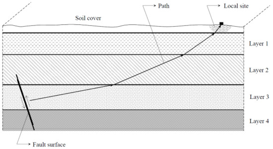
Figure 1.
Physical mechanisms of seismic wave propagation.
The Fourier amplitude and phase spectrum of the acceleration are combined by the Fourier amplitude and phase spectrum of three parts, namely the seismic source, propagation path, and local site, as follows [6,42]:
where Hso (ω), Hpa (ω), His (ω) are the Fourier amplitude of the seismic source, propagation path, and local site, respectively. The subscripts “so, pa, si” mean the seismic source, propagation path, and local site, respectively. Meanwhile, Φso (ω), Φpa (ω), Φsi (ω) are the Fourier phase of the seismic source, propagation path, and local site, respectively.
The seismic source was modeled using the Brune source model [44]. This model assumes that the fault plane is a round plane, the fault dislocations are evenly distributed on the fault plane, and the fault occurs instantaneously. The shear wave generated by the source dislocation propagated in the direction perpendicular to the fault plane, as shown in Figure 2. The near-field displacement induced by fault rupture should be:
where σ is the effective shear stress, β is the shear wave velocity, and μ and τ denote the shear modulus and the Brune source parameter, describing the decay process of the fault rupture, respectively. Let x→0 and transform Equation (4) into the frequency domain, we obtain:
where uso and Uso (ω) are the motions of the seismic source in the time and frequency domains, respectively.
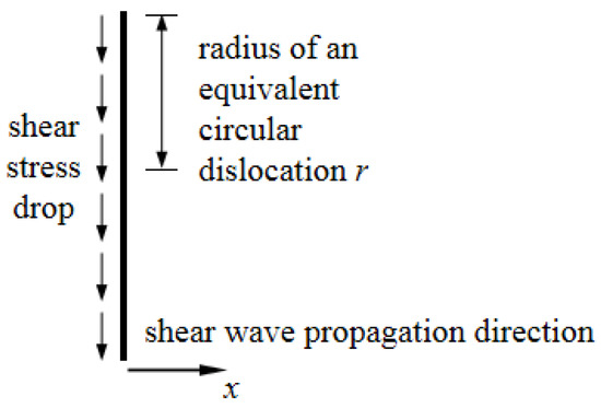
Figure 2.
Schematic of the Brune source model.
The source amplitude spectrum and the phase spectrum should be
where A0 = σβ/μ and τ are the two random parameters of the seismic source, which can be obtained based on many acceleration records in different types of sites. An example has been shown in the literature [5].
The medium from the seismic source to the local site was simplified to a one-dimensional uniform linear elastic medium, and the damping effect and the dispersion effect were considered. At this time, the amplitude spectrum and phase spectrum for the propagation path are simplified as follows [42]:
where K indicates the mean damping effect of the medium and can take a value of 10−5 s/km, R is the epicentral distance, and a, b, c, and d are four empirical parameters. The constants a, b, c, and d in the model are also identified from the recorded acceleration time histories. The detailed process of the identification can be found in the literature [5].
As the influence of the propagation path on the phase spectrum is complicated, after many attempts, Song revised Equation (9) based on the principle that the phase difference distribution between the simulated ground motion and the real earthquake should be as consistent as possible. The modified phase spectrum is as follows [45]:
The local site can be simulated by an equivalent single-degree-of-freedom (SDOF) system, as shown in Figure 3. The input of the system is the seismic wave imposed on the bedrock surface and the displacement of the bedrock is uR. The relative displacement of the system with respect to the bedrock is u, then the absolute displacement of the system uR0 can be obtained by:
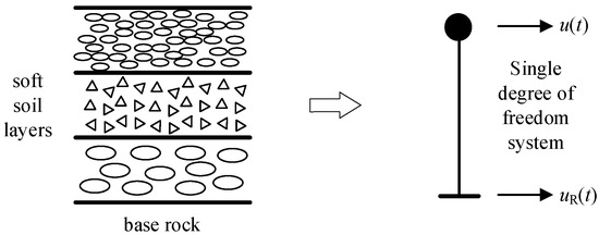
Figure 3.
Equivalent single-degree-of-freedom of the local site.
The kinematic equation of the system is
Equation (12) is easily found in Dynamics of Structures, such as the book written by Chopra [46]. Substituting Equation (12) Into Equation (11) will lead to the motion equation of the system in the time domain as follows:
where uR0 is the output ground motion at a local site. ξg is the equivalent damping ratio of the local site. ωg is the equivalent predominant circular frequency of a local site. Subsequently, according to Equation (13), we can obtain the motion equation of the SDOF system in the frequency domain as follows:
where UR0 (ω) and U0 (ω) are the Fourier transforms of uR0 and uR, respectively, and j is an imaginary unit. Subsequently, we can obtain
Therefore, in the frequency domain, we can obtain the transfer function from UR0 (ω) to U0 (ω) as follows:
where ξg and ωg are the characteristic parameters of the local site.
Therefore, the amplitude spectrum should be equal to:
The phase spectrum of seismic waves in the local site should be
where the symbol “” indicates phase angle calculation. Generally, this is a very small number and represents the phase change from bedrock to the surface. This value is usually ignored by researchers due to its small impact [47].
Lastly, Equations (2) and (3) can be embodied as:
When the vector is a random vector, the ground motion model in Equation (1) becomes a random ground motion model.
The predominant frequency (ωg) and damping ratio (ξg) are obtained according to real seismic acceleration records in different types of sites. An example can be found in the literature [5]. For different types of sites, the histogram and the probability density function of ωg are shown in Figure 4 as an example (herein, PDF is the abbreviation of probability density distribution).
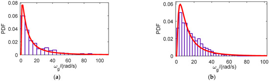
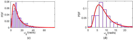
Figure 4.
Histogram and the probability density function of ωg in four kinds of sites: (a) Site I (b) Site II (c) Site III (d) Site IV [5].
In engineering practice, the predominant frequency can also be obtained according to the test of the shear wave velocity (Vs30 in ALA seismic guidelines [48] and Vs20 in Chinese seismic codes [49]). However, the relationship between them is not constant for different sites. Many researchers pay attention to the relationship between the predominant frequency and shear wave velocity, e.g., [50,51].
After we obtain the Fourier amplitude and phase spectrum in Equations (2) and (3), the simulated accelerations in the time domain can be obtained by the inverse discrete Fourier transform method [52] or the method of narrowband wave groups [53].
3. Random Nonstationary Spatially Variable Ground Motion Model
3.1. Model Introduction
Figure 5 is a plan view to show the seismic wave propagation in the local site. The propagation of seismic waves is very complex. Seismic waves can propagate in three dimensions. To simplify this problem and generate stochastic ground motions for engineering practice, many researchers have reduced it to a one-dimensional propagation problem [5]. The propagation direction is defined in a simplified way as the direction of the seismic source toward the local site.
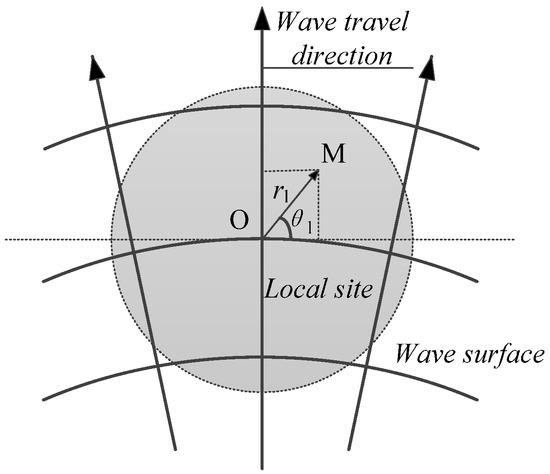
Figure 5.
Seismic wave propagation in the local site (plan view).
Point O is the center point of the local site. Point M is any point at the local site. We assume that the seismic waves travel from point O to point M. Therefore, in the frequency domain, we have:
where HM (ω,r1) and HO (ω,r1) denote the amplitude spectra of seismic waves at points M and O, respectively; ΦM (ω,r1) and ΦO (ω,r1) are the phase spectra of seismic waves at points M and O, respectively, and r1 is the distance between the two points in the direction of seismic wave propagation. Hpr (ω,r1) and Φpr (ω,r1) are the propagation laws of amplitude and phase at the local site, respectively, which can be expressed as follows [43]:
where α0 is the attenuation parameter of the local site, and cg is the apparent seismic wave velocity. α0 and cg are random variables.
However, after careful evaluation, the two shortcomings of that model are: α0 is not self-consistent in this model. According to this assumption, α0 is a constant at different frequencies in this model. However, according to Equations (21) and (23),
Obviously, the parameter α0 should change with frequency, so it is not a constant.
(2) The model only considers the traveling wave effect but neglects the dispersion effect of earthquakes. Herein, the dispersion effect refers to the phenomenon wherein waves with different frequencies propagate at different speeds.
In fact, seismic waves not only have obvious traveling wave effects but also present prominent dispersion effects even at a relatively uniform site. To verify these two phenomena, the accelerations tested by the SMART-1 array were selected as an example. The layout and number of different stations in the array are shown in Figure 6. The distance between stations C00 and I06 in the east–west direction is approximately 45.5 m. The accelerations tested by these two stations in Event 5 in the east–west direction are shown in Figure 7a. Figure 7a shows that, in the real earthquake field, the traveling wave effect is obvious. A comparison of the frequency spectra is shown in Figure 7b. Accordingly, the difference between the two frequency spectra is also obvious. Therefore, the dispersion effect is also prominent, although the distance between these two stations in the east–west direction is only 45.5 m.
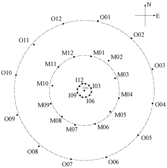
Figure 6.
The SMART-1 array.
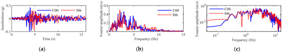
Figure 7.
(a) Accelerations tested by SMART-1. (b) Fourier spectra of the accelerations. (c) Fourier spectra of the accelerations on a log-log scale.
However, because the apparent seismic wave velocity cg in this model is constant, the simulated acceleration in the frequency at different points does not change much. Herein, the model was used to produce samples for the site shown in Figure 8. Point PO was at the center of the site. Point PA represents a point along the direction of seismic wave propagation. It is 45.5 m away from point PO. The simulated accelerations and their Fourier spectra are shown in Figure 9. Obviously, in the simulated field, the traveling wave effect is obvious, according to Figure 9a, whereas in Figure 9b, the dispersion effect is neglected.
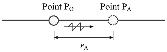
Figure 8.
A simple seismic field.
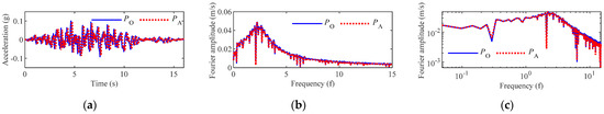
Figure 9.
(a) Simulated accelerations. (b) Fourier spectra of the simulated accelerations. (c) Fourier spectra of the accelerations on a log–log scale.
3.2. Model Modification
To solve the above-mentioned two problems, the amplitude and phase spectra were improved.
3.2.1. Modification of the Amplitude Spectrum
Equation (23) is used to describe the change law of the Fourier amplitude spectrum: However, parameter α should change with frequency as follows:
where Fα is a function that needs to be determined.
Herein, the accelerations in Figure 7 are taken as an example to study the function Fα. The accelerations and their Fourier amplitude spectra are shown in Figure 7. For the convenience of modeling, only records from 0 to 16 s were removed. Subsequently, based on Equation (25), parameter α can be obtained as follows:
where and are the amplitude spectra of the seismic waves at stations C00 and I06, respectively. r0 is the distance between the two stations in the east–west direction and takes a value of 0.0455 km. Figure 10 shows that the parameter changes severely, especially at low frequencies. Therefore, the following function is used to describe the parameters:
where ω (rad) is the circular frequency. p1, p2, and p3 are the three parameters. For the function in Figure 10, the three corresponding numbers of p1, p2, p3 are 19.6300, 9.4480, and −0.0695. The coefficient of correlation is 0.9142. Since the amplitude of the acceleration in the frequency domain is very small after 15 Hz (Figure 7), only the acceleration in the range of 0–15 Hz is utilized for the parameter identification in this paper. Due to the scarcity of data from strong motion arrays, only the data of event 5 obtained by SMART-1 are used.
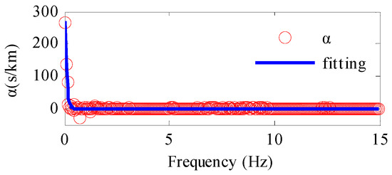
Figure 10.
Fitting of parameter α.
3.2.2. Modification Law of the Phase Spectrum
To describe the dispersion effect of seismic waves, we assumed that the seismic velocity changes with frequency as follows:
where Fcg is a function that must be determined. This hypothesis regards soil as a dispersive medium. This is in accordance with the fact that the soil is essentially a type of viscoelastic medium with damping [54].
To obtain the function Fcg, the method suggested by Loh was utilized [55]. The main steps are as follows:
At frequency ω0, the accelerations at the two stations should be filtered by a narrowband filter. The filter is a Butterworth bandpass filter with a bandwidth of π rad/s. Subsequently, two narrowband accelerations can be obtained as follows:
where a1 and a2 are the initial acceleration while and are the filtered acceleration at the frequency ω0, respectively; F and F−1 are the Fourier transform and the inverse Fourier transform, respectively; is a narrowband filter, and its mid-frequency is ω0; the symbol “∣·∣” indicates capturing the Fourier transform module. In addition, for avoiding the phase delay of accelerations during filtering, a zero-phase digital filtering method is recommended [56].
The cross-correlation of and can be expressed as
where is the cross-correlation between and . Generally, when reaches its maximum, the value is the delay time between the two signals and . However, at the local site, the propagation direction should be considered. Therefore, the delay time should be determined, according to the following rules:
(1) When the seismic waves propagate from to , the delay time should be
where τ1 is the delay time obtained according to the cross-correlation when the seismic waves propagate from to . Now, τ1 should satisfy the following conditions:
where Rpeak1 is the first peak value of Ra (τ) when τ is positive.
(2) When the seismic waves propagate from to , the delay time should be
where τ2 is the delay time obtained according to the cross-correlation when the seismic waves propagate from to . At this time, τ2 should satisfy the following conditions:
where Rpeak2 is the first peak value of Ra (τ) when τ is negative.
(3) The seismic velocity at frequency ω0 can be obtained by
Moreover, the seismic velocity should satisfy the closure property [57]. As shown in Figure 11, three stations, S1, S2, and S3, are arranged in a field. The distances between the two stations along the wave propagation direction were d12, d23, and d13. For a plane wave at a specific frequency, the closure property can be expressed as follows:
where vse is the velocity of the plane wave.
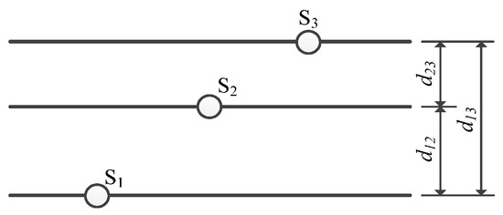
Figure 11.
Closure property for a plane wave.
The accelerations at stations C00 and I06 in Event 5 were studied as an example to obtain the seismic wave velocities at different frequencies, based on the methods suggested above.
(1) When the frequency ω0 is 0.8 Hz, the filtered accelerations are shown in Figure 12a. Subsequently, the cross-correlation between them can be obtained, as shown in Figure 12b. Accordingly, the first extreme point is Q1 when τ is positive. Therefore, the delay time should be 0.64 s. Then, the seismic wave velocity should be:
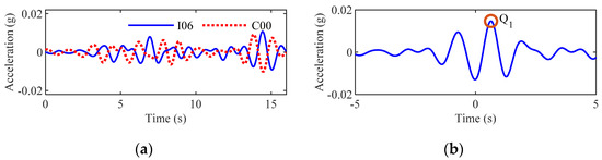
Figure 12.
(a) Filtered accelerations for accelerations at stations I06 and C00 when ω0 = 0.8 Hz, and (b) cross-correlation of the filtered accelerations.
(2) When the frequency ω0 is 2 Hz, based on the same process, as shown above, the filtered accelerations and cross-correlation are shown in Figure 13. At this moment, the delay time should be 0.2 s. Consequently, the seismic wave velocity should be 0.2275 km/s.
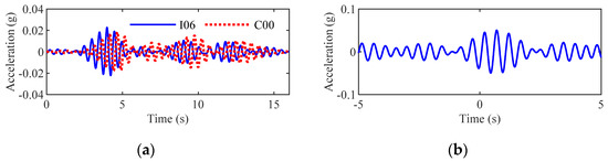
Figure 13.
(a) Filtered accelerations for accelerations at stations I06 and C00 when ω0 = 2 Hz; (b) cross-correlation of the filtered accelerations.
The seismic wave velocities should be examined. When the frequency ω0 is 2 Hz, the accelerations at stations I06, C00, and I12 in the east–west direction can be used to verify each other. The filtered accelerations and the corresponding cross-correlation at stations C00 and I12, I06 and I12 are shown in Figure 14 and Figure 15, respectively.
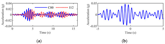
Figure 14.
(a) Filtered accelerations for accelerations at stations C00 and I12 when ω0 = 2 Hz, and (b) cross-correlation of the filtered accelerations.
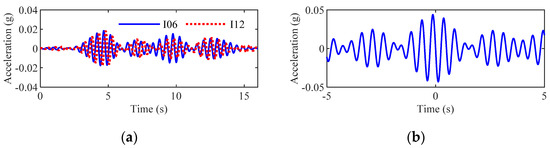
Figure 15.
(a) Filtered accelerations for accelerations at stations I06 and I12 when ω0 = 2 Hz, and (b) cross-correlation of the filtered accelerations.
According to Figure 14 and Figure 15, the delay time from station C00 to station I12 is 0.18 s, and the delay time from station I06 to station I12 is 0.37 s. Therefore, we obtain
where τI06-C00, τC00-I12, and τI06-I12 denote the delay times of seismic waves from stations I06, C00, and I06 to stations C00, I12, and I12, respectively.
Meanwhile, based on Equation (38), the delay time from station I06 to station I12 should be
The relative error between and is 2.63%; therefore, it can be assumed that the seismic velocity meets the closure property successfully.
(1) According to the procedure shown in (1) and (2), we can obtain the seismic wave velocities at different frequencies from station I06 to station C00 in the east–west direction, as shown in Figure 16. Consequently, an obvious linearly increasing trend can be observed in Figure 16. Therefore, the function Fcg in Figure 16 can be represented by a linear function as follows:
where q1 and q2 are the two parameters to be determined. For the function in Figure 16, the parameters q1 and q2 are 0.07273 and 0.09343, respectively. Figure 16 is used to illustrate how the parameters q1 and q2 are obtained for a set of ground motions in two sites. The results in Figure 16 are illustrated with ground motion records in I06 and C00. For other ground motion records, the treatment is similar. Thus, we can obtain many sets of parameters q1 and q2 to determine the distribution information. For the convenience of data processing, we uniformly intercepted the information of seismic waves from 0 to 15 Hz for analysis.
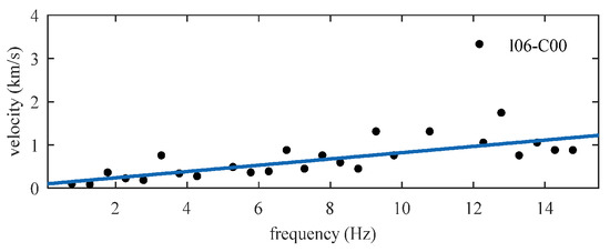
Figure 16.
Seismic velocity at different frequencies.
(2) Figure 10, Figure 11, Figure 12, Figure 13, Figure 14, Figure 15 and Figure 16 are used as examples to illustrate how parameters p1, p2, p3, q1, q2 can be obtained from a group of ground motion records (I06-C00). For other groups of ground motion records, such as (I12-C00), the process to obtain these five parameters is similar. The ground motion records are the test records from the SMART-1 array in the PEER database. The parameters may be correlated with each other. However, for simplicity of processing, those parameters are supposed to be independent when the number of ground motion records is very large. Because these five parameters are derived from the amplitude and phase spectra of seismic wave propagation in the local site, they do not consider the characteristics of the seismic sources and propagation paths, but only the propagation of seismic waves within the local site.
3.2.3. Revised Model
Based on the amendment of the amplitude and phase transfer functions in the frequency domain mentioned above, the new model in the frequency domain can be expressed as follows:
Herein, p1, p2, p3, and q1, q2 denote parameters related to the local site. Obviously, when these parameters are random, the model becomes a random ground motion model.
3.3. Model Parameters
To build a random seismic field, the parameters p1, p2, p3, q1, and q2 in Equations (48) and (49) need to be statistically modeled. Herein, the accelerations obtained by SMART-1 in the east–west and south–north directions were analyzed. For a specific pair of acceleration records in the same site, such as I06 and C00, the parameters are constant. However, for different pairs of acceleration records in the same site, these five variables are random. We obtain five groups of parameter values by analyzing many pairs of acceleration records. They are supposed to be independent in many samples. Thus, a stochastic ground model can be established.
For a pair of specific stations, there is a certain correlation between parameters p1–p3 or q1–q2. When we identify those parameters, we always obtain them group by group. However, we ignore the correlation between parameters when there are many samples because it is difficult to describe the correlation between such parameters. At the same time, ignoring this correlation is very convenient for the sample generation of random variables. This method is also a common method for many artificial earthquake models. For example, in many models, the phase angle is assumed to be an independent random variable [53], or in the lagged coherency of spatially variable ground motion models, the phase angle difference between two stations fits some random distribution [33]. We were not able to study the probability distribution of these five parameters in the model in other types of sites due to the paucity of sample data.
3.3.1. Parameters of the Amplitude Spectrum
For the parameters in Equation (28), according to the method in Section 3.2.1, the parameters p1, p2, and p3 for the accelerations in the east–west and south–north directions can be obtained. The distribution patterns of these parameters are studied. The parameter q1 satisfies the exponential distribution as follows:
Parameters q2 and q3 satisfy the normal distribution as follows:
Herein, parameters λ, μ, and σ are parameters in the probability density function and are summarized in Table 1, where λ is the rate parameter of the exponential distribution function, and μ and σ are the mean and standard deviation of the normal distribution, respectively. The distribution fittings of these parameters are shown in Figure 17. All distribution fittings were tested by the KS test, and the confidence levels were all 95%.

Table 1.
Probability distribution of parameters in the amplitude and phase transfer functions.
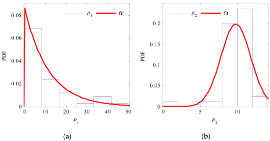
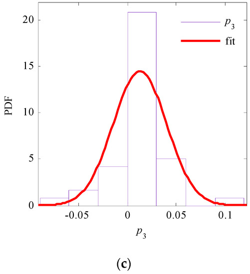
Figure 17.
Distribution fitting of parameters (a) p1 and (b) p2 and (c) p3 in the amplitude transfer function.
3.3.2. Parameters of the Phase Spectrum
For the parameters in Equation (47), according to the method in Section 3.2.2, the parameters can be obtained based on the accelerations in the east–west and south–north directions. The distribution fittings of the two parameters are shown in Figure 18. Herein, an exponential function is used to fit the probability density distribution. The probability distribution information for these two parameters is summarized in Table 1. In addition, all distributions were tested using the KS test, and the confidence levels were as high as 95%.
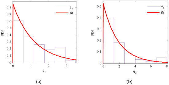
Figure 18.
Distribution fitting of (a) parameter q1 and (b) parameter q2 in the phase transfer function.
3.4. Generation of Spatially Variable Ground Motions
Finally, the new spatially variable ground motion model is expressed as follows:
where aRS (rl,t) is the acceleration at any point in the modeling field, and is a random vector. For completeness and convenience, the probability distribution types and corresponding distribution information of the four parameters are listed in Table 2. The ground motion model proposed in this paper is modeled in the frequency domain by considering the seismic source, propagation path, and local site separately. The randomness of the parameters in the source and propagation path has been presented in the literature [5,42,58], and this paper only focuses on the randomness of the seismic wave propagation in the local site. For a specific acceleration record, the parameters are correlated. However, for many acceleration records, the parameters are assumed to be independent to facilitate engineering applications.
Table 2.
Probability distribution of random parameters.
The model parameters were fitted to acceleration samples from a single event recorded by the SMART-1 array. The probability distribution of those model parameters is, therefore, specific to that event and that region. However, it is a reasonable assumption to apply these parameters to the simulation of seismic waves in the same types of sites, according to the American and Chinese seismic guidelines. For other types of sites, it should be noted that the values of these parameters are not applicable and more ground motion samples from more events and different kinds of sites may be required to obtain appropriate parameters.
To produce a random local field, the following algorithm steps should be taken:
(1) Determine the peak ground acceleration (PGA) and the number of samples needed. For example, for an ordinary residential house located in Beijing, the PGA is usually required to be 0.2 g, according to the seismic codes. The number of samples needs to be determined, according to the reliability assessment method.
(2) Build a coordinate system at the local site and determine the coordinates of the different simulated points. For simplicity, the origin of the coordinate can be assumed to be the incident point of the seismic waves, traveling from the bedrock to the surface of the site.
(3) Determine the probability distribution information of the nine random parameters, according to Table 1 and Table 2. Subsequently, sample points are generated based on different sampling methods, such as the multiplicative congruential method or the mixed congruential method.
(4) The simulated accelerations in the frequency domain at different points in the site can be obtained based on the coordinates of different points in the local site and the selected sample points.
(5) The inverse discrete Fourier transform method [43] or the method of narrowband wave groups [44] can be utilized to obtain accelerations in the time domain. The amplitude of the acceleration at the origin of the coordinate should be modulated according to the amplitude of the designed acceleration. Subsequently, the amplitude of the accelerations at other locations in the local site should be modulated according to the same ratio. The modulation of the acceleration amplitude is based on the peak value of the design acceleration. For example, if the peak value of the design acceleration is 0.2 g while the peak value of the simulated acceleration is 100 m/s2, then the simulated acceleration needs to be divided by 100 m/s2 and multiplied by 0.2 g to get the design acceleration. In the frequency domain, the Fourier amplitude and phase spectrum depend on the source, path, and/or site characteristics.
The above process is also shown schematically in Figure 19.
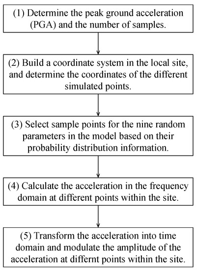
Figure 19.
Flowchart to show the application of the proposed model.
We have compared the simulated acceleration C00 and I06 with the tested acceleration C00 and I06, as shown in Figure 20. The corresponding parameters of the numerical model of C00 is as follows: A0 = 0.1512 (g·s/rad), τ = 0.2084 (s/rad), ζg = 0.2776 rad, ωg = 19.2637 rad, a = 3262.0044, b = 355.9342 rad/s, c = 3804.2735 s/rad, d = 8272.1111 rad/m. The simulated acceleration I06 is obtained, according to the site model introduced in Equations (48) and (49).
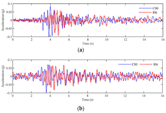
Figure 20.
Comparison between measured and simulated acceleration: (a) Tested acceleration C00 and I06. (b) Simulated acceleration C00 and I06.
Accordingly, it can be found that the simulated acceleration curves have some similarities with the measured acceleration curves, especially the envelope of the acceleration curves. For station C00, the peak value of the measured acceleration occurs at 3.85 s (−0.1 g) while the peak value of the simulated acceleration occurs at 3.59 s (−0.1 g). For station I06, the peak value of the measured acceleration occurs at 4.85 s (−0.09252 g) while the peak value of the simulated acceleration occurs at 4.42 s (−0.08134 g). Therefore, for the measured acceleration, the time between the appearance of peak values (C00-I06) is 1 s while for the simulated acceleration, the time between the appearance of peak values (C00-I06) is 0.93 s. Both the measured and simulated acceleration exhibits a relatively significant wave passage effect. In addition, the Pearson correlation coefficient between the two measured acceleration curves is 0.0410 while the Pearson correlation coefficient between the two simulated acceleration curves is −0.0692. Thus, both the measured and simulated acceleration curves exhibit a significant dispersion phenomenon.
3.5. Examples of Spatially Variable Ground Motions
3.5.1. Example 1
To illustrate the model, the site shown in Figure 8 is used as an example. Herein, we suppose that this site is a type-II site, according to the Chinese seismic design code, with a shear wave velocity of 250 m/s [49]. In this example, a coordinate system is built, as shown in Figure 8. The origin of the coordinate is point PO. The distance between the points PA and PO was 1000 m. The site is a type-II site; therefore, the probability distribution information of the nine random parameters can be obtained according to Table 1 and Table 2, respectively. A total of 5000 sample points can be obtained to simulate 5000 different seismic field samples. Herein, Figure 21 is used as an example to show the sample points and the corresponding probability density distribution of the points for parameter p1.
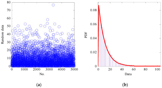
Figure 21.
(a) Sample points and (b) probability density distribution of the points for parameter p1.
Subsequently, the accelerations at different points in the field can be determined, according to Equations (52)–(54). The accelerations and the corresponding displacements at point PO and point PA in the first three samples are shown in Figure 22, Figure 23 and Figure 24, respectively. Accordingly, the simulated accelerations and the corresponding displacements at points PO and PA not only have an obvious traveling effect but also exhibit a prominent dispersion effect. However, for different samples, the obviousness of the two effects is different. For example, in sample 2, the dispersion effect is very weak; therefore, the seismic waves mainly show the traveling effect, whereas, in samples 1 and 3, the traveling and dispersion effects are both obvious.
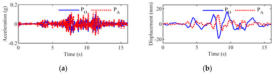
Figure 22.
Accelerations and displacements in sample 1: (a) simulated accelerations and (b) its corresponding displacements.
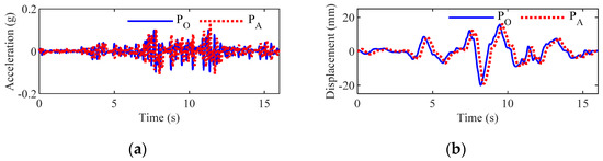
Figure 23.
Accelerations and displacements in sample 2: (a) simulated accelerations and (b) its corresponding displacements.
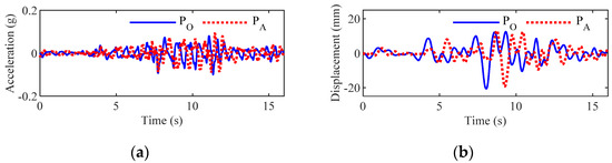
Figure 24.
Accelerations and displacements in sample 3: (a) simulated accelerations and (b) its corresponding displacements.
3.5.2. Example 2
A continuous random field of ground motion was generated to illustrate the dispersion effect of the proposed model. The propagation distance of the seismic wave is defined as 1000 m. For the simulation, p1, p2, and p3, which affect the attenuation parameter, are sampled as 8.47, 10.52, and 0.01, respectively; q1 and q2, which affect the apparent wave velocity, were sampled as 0.98 and 1.50, respectively. (In Example 2, it is supposed that this site meets one group of parameters identified from a specific group of stations. This is because the relative distance between stations is fixed, and the parameter values between different groups of stations are different and cannot be used to generate a continuous seismic wave field.) The distance interval of the time history samples is 4 m along the direction of wave propagation. The time interval of time history samples equals 0.02 s along the time axis. The generated random field of ground motion is shown in Figure 24, where the dispersion effect in the ground motion field is reproduced. It should be noted that Figure 25 represents the spatially variable ground motions in three-dimensional space, which reflects the change of ground motions with time and space. If we make a slice perpendicular to the time axis, the graph is the variation of the acceleration over a certain range (1000 m). Similarly, if we make a slice perpendicular to the space axis, the graph is the variation of the acceleration over a certain time (22.50 s).
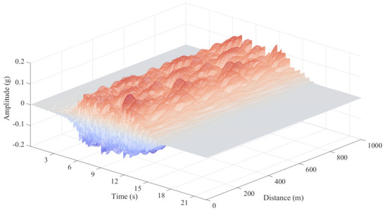
Figure 25.
Generated random field of ground motion by the proposed model.
A top view of the generated field is shown in Figure 25. Wave passage and dispersion effects can be observed. Figure 26 shows the evolution of the amplitude of the ground motion field with distance. The attenuation effect is not obvious, owing to the short propagation distance and the interference of the dispersion effect, but a slight attenuating trend can be observed.
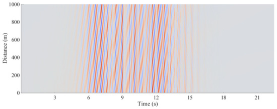
Figure 26.
Evolution of the shape of ground motion field with distance.
It should be noted that ground motion prediction equation curves, e.g., ASK14 [59], mainly focus on the attenuation of earthquakes in a relatively large area. When those models are built, the seismic records tested by a seismic array in a local area are not used. Therefore, those models can hardly reflect the change law of seismic waves in a local site. The model presented in this paper is to describe the spatial variability of ground motions in a local site. Works with the same objective are [60,61]. This paper focuses on the variability of ground motions in a local site based on SMART-1 array data. In addition, it should be noted that the stations in SMART-1 can only test the ground motions at some special points in the local site while it cannot obtain continuous ground motions in the spatial dimension, as shown in Figure 25, Figure 26, Figure 27 and Figure 28.
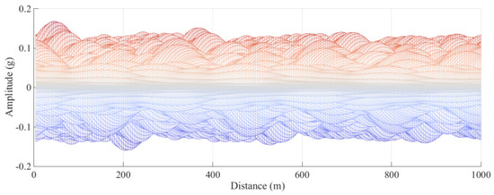
Figure 27.
Evolution of the amplitude of ground motion field with distance.
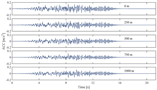
Figure 28.
Changes in seismic waves at different distance.
The suggested model has the following advantages. (1) The new model has a very clear physical background based on the propagation law of seismic waves. (2) The new model avoids the Cholesky decomposition of the cross-spectral density matrix or the iterative loop in the conditional simulation. The Fourier amplitude spectrum and phase spectrum at every simulated point in the local site can be directly obtained. Therefore, it is very convenient for engineering applications.
4. Conclusions
A new random nonstationary spatially variable ground motion model for engineering applications was proposed herein. The model is built according to the propagation law of seismic waves, which are supposed to travel from the hypocenter to the local site. The following conclusions were drawn:
(1) Accelerations tested by the SMART-1 array show that even for relatively short distances in the local site, the seismic waves demonstrate significant dispersion. Therefore, a suitable model should not only reflect the traveling wave effect of seismic waves but also exhibit the dispersion effect.
(2) The new model establishes expressions in the frequency domain for the seismic source, propagation path, and local site. It has a clear physical background and is extremely easy to understand. Meanwhile, the new model avoids the Cholesky decomposition of the cross-spectral density matrix or the iterative loop in the conditional simulation. The Fourier amplitude spectrum and phase spectrum at every simulated point in the local site can be directly obtained. Therefore, it is very convenient for engineering applications.
(3) The numerical case shows that the accelerations in different samples have different characteristics, even for the same site, owing to randomness. In some samples, the traveling wave effect was more pronounced than the dispersion effect, whereas in other samples, the latter is more obvious than the former. The example also shows the practicality of the new model.
In addition, seismic waves in free terrain or built-up areas seem to be different, which may also be an interesting topic. In this paper, we only focus on the generation of ground motions without considering the impact of buildings [62]. Therefore, we first generate seismic waves according to the equations proposed in the paper and then apply them to building structures, such as bridges, pipelines, and building portfolios.
Author Contributions
Conceptualization, H.M.; methodology, Y.D. and H.M.; software, H.M.; validation, H.M.; formal analysis, H.M.; investigation, Y.D.; resources, Y.D.; data curation, H.M.; writing—original draft preparation, H.M.; writing—review and editing, H.M. and J.S.; visualization, H.M. and J.S.; supervision, Y.D. and J.S.; project administration, H.M.; funding acquisition, H.M. All authors have read and agreed to the published version of the manuscript.
Funding
This research was funded by the Beijing Natural Science Foundation (Grant No. 8222008), the National Natural Science Foundation of China (Grant No. 52108427), and the China Postdoctoral Science Foundation (Grant No. 2021M690278).
Institutional Review Board Statement
Not applicable.
Informed Consent Statement
Not applicable.
Data Availability Statement
Not applicable.
Acknowledgments
Funding from the Beijing Natural Science Foundation (Grant No. 8222008), the National Natural Science Foundation of China (Grant No. 52108427), and the China Postdoctoral Science Foundation (Grant No. 2021M690278) is highly appreciated. All the accelerograms used in this study are downloaded from the website of the Pacific earthquake engineering research center (PEER), http://ngawest2.berkeley.edu (accessed on 1 April 2018) The authors are also grateful to the PEER.
Conflicts of Interest
The authors declare no conflict of interest.
References
- Otani, S. The dawn of structural earthquake engineering in Japan. In Proceedings of the 14th World Conference on Earthquake Engineering, Beijing, China, 12–17 October 2008; ASCE: Reston, VA, USA; pp. 1–8. [Google Scholar]
- Reitherman, R.K. Earthquakes and Engineers: An International History; ASCE: Reston, VA, USA, 2012. [Google Scholar]
- Housner, G.W. Characteristics of strong-motion earthquakes. Bull. Seism. Soc. Am. 1947, 37, 19–31. [Google Scholar] [CrossRef]
- Housner, G.W. Properties of strong ground motion earthquakes. Bull. Seism. Soc. Am. 1955, 45, 197–218. [Google Scholar] [CrossRef]
- Ding, Y.; Peng, Y.; Li, J. A Stochastic semi-physical model of seismic ground motions in time domain. J. Earthq. Tsunami 2018, 12, 1850006. [Google Scholar] [CrossRef]
- Boore, D.M. Simulation of ground motion using the stochastic method. Pure Appl. Geophys. 2003, 160, 635–676. [Google Scholar] [CrossRef]
- Boore, D.M.; Atkinson, G.M. Ground-motion prediction equations for the average horizontal component of PGA, PGV, and 5%-damped PSA at spectral periods between 0.01 s and 10.0 s. Earthq. Spectra 2008, 24, 99–138. [Google Scholar] [CrossRef]
- Boore, D.M.; Thompson, E. Path Durations for use in the stochastic-method simulation of ground motions. Bull. Seism. Soc. Am. 2014, 104, 2541–2552. [Google Scholar] [CrossRef]
- Boore, D.M.; Thompson, E.M. Revisions to some parameters used in stochastic-method simulations of ground motion. Bull. Seism. Soc. Am. 2015, 105, 1029–1041. [Google Scholar] [CrossRef]
- Ktenidou, O.; Cotton, F.; Abrahamson, N.A.; Anderson, J.G. Taxonomy of κ: A Review of definitions and estimation approaches targeted to applications. Seism. Res. Lett. 2014, 85, 135–146. [Google Scholar] [CrossRef]
- Boore, D.M. Comparing Stochastic point-source and finite-source ground-motion simulations: SMSIM and EXSIM. Bull. Seism. Soc. Am. 2009, 99, 3202–3216. [Google Scholar] [CrossRef]
- Motazedian, D. Stochastic Finite-Fault Modeling based on a dynamic corner frequency. Bull. Seism. Soc. Am. 2005, 95, 995–1010. [Google Scholar] [CrossRef]
- Campbell, K.W.; Bozorgnia, Y. NGA Ground motion model for the geometric mean horizontal component of PGA, PGV, PGD and 5% damped linear elastic response spectra for periods ranging from 0.01 to 10 s. Earthq. Spectra 2008, 24, 139–171. [Google Scholar] [CrossRef]
- Campbell, K.W.; Bozorgnia, Y. NGA-West2 ground motion model for the average horizontal components of PGA, PGV, and 5% damped linear acceleration response spectra. Earthq. Spectra 2014, 30, 1087–1115. [Google Scholar] [CrossRef]
- Vlachos, C.; Papakonstantinou, K.G.; Deodatis, G. A multi-modal analytical non-stationary spectral model for characterization and stochastic simulation of earthquake ground motions. Soil Dyn. Earthq. Eng. 2016, 80, 177–191. [Google Scholar] [CrossRef]
- Rezaeian, S.; Kiureghian, A.D. Simulation of synthetic ground motions for specified earthquake and site characteristics. Earthq. Eng. Struct. Dyn. 2010, 39, 1155–1180. [Google Scholar] [CrossRef]
- Liu, Z.; Liu, W.; Peng, Y. Random function based spectral representation of stationary and non-stationary stochastic processes. Probabilistic Eng. Mech. 2016, 45, 115–126. [Google Scholar] [CrossRef]
- Svay, A.; Perron, V.; Imtiaz, A.; Zentner, I.; Cottereau, R.; Clouteau, D.; Bard, P.-Y.; Hollender, F.; Lopez-Caballero, F. Spatial coherency analysis of seismic ground motions from a rock site dense array implemented during the Kefalonia 2014 aftershock sequence. Earthq. Eng. Struct. Dyn. 2017, 46, 1895–1917. [Google Scholar] [CrossRef]
- Luco, J.E.; Wong, H.L. Response of a rigid foundation to a spatially random ground motion. Earthq. Eng. Struct. Dyn. 1986, 14, 891–908. [Google Scholar] [CrossRef]
- Jeremić, B.; Tafazzoli, N.; Ancheta, T.; Orbović, N.; Blahoianu, A. Seismic behavior of NPP structures subjected to realistic 3D, inclined seismic motions, in variable layered soil/rock, on surface or embedded foundations. Nucl. Eng. Des. 2013, 265, 85–94. [Google Scholar] [CrossRef]
- Hao, H. Arch responses to correlated multiple excitations. Earthq. Eng. Struct. Dyn. 1993, 22, 389–404. [Google Scholar] [CrossRef]
- Bi, K.; Hao, H. Simulation of spatially varying ground motions with non-uniform intensities and frequency content. In Proceedings of the Australian Earthquake Engineering Society Conference, Ballarat, VIC, Australia, 17–18 October 2002. [Google Scholar]
- Bi, K.; Hao, H.; Li, C.; Li, H. Stochastic seismic response analysis of buried onshore and offshore pipelines. Soil Dyn. Earthq. Eng. 2017, 94, 60–65. [Google Scholar] [CrossRef]
- Saxena, V.; Deodatis, G.; Shinozuka, M. Effect of spatial variation of earthquake ground motion on the nonlinear dynamic response of highway bridges. In Proceedings of the 12th World Conference on Earthquake Engineering, Auckland, New Zealand, 30 January–4 February 2000; ASCE: Reston, VA, USA; pp. 1–8. [Google Scholar]
- Léger, P.; Idé, I.; Paultre, P. Multiple-support seismic analysis of large structures. Comput. Struct. 1990, 36, 1153–1158. [Google Scholar] [CrossRef]
- Wilson, E.L. Three Dimensional Static and Dynamic Analysis of Structures, 3rd ed.; Computers and Structures, Inc.: Berkeley, CA, USA, 2002. [Google Scholar]
- Heredia-Zavoni, E.; Vanmarcke, E.H. Seismic random-vibration analysis of multisupport-structural systems. J. Eng. Mech. 1994, 120, 1107–1128. [Google Scholar] [CrossRef]
- Abrahamson, N.A.; Bolt, B.A.; Darragh, R.B.; Penzien, J.; Tsai, Y.B. The SMART I accelerograph array (1980–1987): A review. Earthq. Spectra 1987, 3, 263–287. [Google Scholar] [CrossRef]
- Chiu, H.-C.; Yeh, Y.T.; Lee, S.-D.N.L.; Liu, W.-H.; Wen, G.-F.; Liu, C.-C. A New Strong-motion array in Taiwan: SMART-2. Terr. Atmospheric Ocean. Sci. 1994, 5, 463–475. [Google Scholar] [CrossRef]
- Katayama, T. Use of dense array data in the determination of engineering properties of strong motions. Struct. Saf. 1991, 10, 27–51. [Google Scholar] [CrossRef]
- Liao, S.; Zerva, A. Physically compliant, conditionally simulated spatially variable seismic ground motions for performance-based design. Earthq. Eng. Struct. Dyn. 2006, 35, 891–919. [Google Scholar] [CrossRef]
- Hao, H.; Oliveira, C.; Penzien, J. Multiple-station ground motion processing and simulation based on SMART-1 array data. Nucl. Eng. Des. 1989, 111, 293–310. [Google Scholar] [CrossRef]
- Zerva, A.; Zervas, V. Spatial variation of seismic ground motions: An overview. Appl. Mech. Rev. 2002, 55, 271–297. [Google Scholar] [CrossRef]
- Deodatis, G. Simulation of ergodic multivariate stochastic processes. J. Eng. Mech. 1996, 122, 778–787. [Google Scholar] [CrossRef]
- Shrikhande, M.; Gupta, V.K. Synthesizing ensembles of spatially correlated accelerograms. J. Eng. Mech. 1998, 124, 1185–1192. [Google Scholar] [CrossRef]
- Vanmarcke, E.H.; Fenton, G.A. Conditioned simulation of local fields of earthquake ground motion. Struct. Saf. 1991, 10, 247–264. [Google Scholar] [CrossRef]
- Vanmarcke, E.H.; Heredia-Zavoni, E.; Fenton, G.A. Conditional simulation of spatially correlated earthquake ground motion. J. Eng. Mech. 1993, 119, 2333–2352. [Google Scholar] [CrossRef]
- Jankowski, R.; Wilde, K. A simple method of conditional random field simulation of ground motions for long structures. Eng. Struct. 2000, 22, 552–561. [Google Scholar] [CrossRef]
- Konakli, K.; Kiureghian, A.D. Simulation of spatially varying ground motions including incoherence, wave-passage and differential site-response effects. Earthq. Eng. Struct. Dyn. 2012, 41, 495–513. [Google Scholar] [CrossRef]
- Dinh, V.-N.; Basu, B.; Brinkgreve, R.B.J. Wavelet-based evolutionary response of multispan structures including wave-passage and site-response effects. J. Eng. Mech. 2014, 140, 04014056. [Google Scholar] [CrossRef]
- Camacho, V.T.; Guerreiro, L.; Oliveira, C.S.; Lopes, M. Effect of spatial variability of seismic strong motions on long regular and irregular slab-girder RC bridges. Bull. Earthq. Eng. 2020, 19, 767–804. [Google Scholar] [CrossRef]
- Wang, D.; Li, J. Physical random function model of ground motions for engineering purposes. Sci. China Technol. Sci. 2010, 54, 175–182. [Google Scholar] [CrossRef]
- Wang, D.; Li, J. A random physical model of seismic ground motion field on local engineering site. Sci. China Technol. Sci. 2012, 55, 2057–2065. [Google Scholar] [CrossRef]
- Brune, J.N. Tectonic stress and the spectra of seismic shear waves from earthquakes. J. Geophys. Res. Earth Surf. 1970, 75, 4997–5009. [Google Scholar] [CrossRef]
- Song, M. Studying Random Function Model of Seismic Ground Motion for Engineering Purposes; Tongji University: Shanghai, China, 2013. (In Chinese) [Google Scholar]
- Chopra, A.K. Dynamics of Structures: Theory and Applications to Earthquake Engineering, 4th ed.; Prentice Hall: Upper Saddle River, NJ, USA, 2012. [Google Scholar]
- Clough, R.W.; Penzien, J. Dynamics of Structures, 3rd ed.; Computers & Structures, Inc.: Berkeley, CA, USA, 2003; p. 94704. [Google Scholar] [CrossRef][Green Version]
- ALA. Seismic Guidelines for Water Pipelines; ASCE; FEMA; NIBS: Washington, DC, USA, 2005.
- Ministry of Construction of the PRC; AQSIQ. Code for Seismic Design of Outdoor Water Supply, Sewerage, Gas and Heating Engineering; China Architecture & Building Press: Beijing, China, 2003.
- Hassani, B.; Atkinson, G.M. Applicability of the site fundamental frequency as a VS30 proxy for central and eastern north America. Bull. Seism. Soc. Am. 2016, 106, 653–664. [Google Scholar] [CrossRef]
- Wang, S.; Shi, Y.; Jiang, W.; Yao, E.; Miao, Y. Estimating site fundamental period from shear-wave velocity profile. Bull. Seism. Soc. Am. 2018, 108, 3431–3445. [Google Scholar] [CrossRef]
- Thráinsson, H.; Kiremidjian, A.S. Simulation of digital earthquake accelerograms using the inverse discrete Fourier transform. Earthq. Eng. Struct. Dyn. 2002, 31, 2023–2048. [Google Scholar] [CrossRef]
- Wong, H.L.; Trifunac, M.D. Generation of artificial strong motion accelerograms. Earthq. Eng. Struct. Dyn. 1979, 7, 509–527. [Google Scholar] [CrossRef]
- Veletsos, A.S.; Verbič, B. Vibration of viscoelastic foundations. Earthq. Eng. Struct. Dyn. 1973, 2, 87–102. [Google Scholar] [CrossRef]
- Loh, C.H. Analysis of the spatial variation of seismic waves and ground movements from smart-1 array data. Earthq. Eng. Struct. Dyn. 1985, 13, 561–581. [Google Scholar] [CrossRef]
- MathWorks. Zero-Phase Digital Filtering—MATLAB Filtfilt. 2022. Available online: https://ww2.mathworks.cn/help/signal/ref/filtfilt.html (accessed on 10 February 2022).
- Boissières, H.-P.; Vanmarcke, E.H. Estimation of lags for a seismograph array: Wave propagation and composite correlation. Soil Dyn. Earthq. Eng. 1995, 14, 5–22. [Google Scholar] [CrossRef]
- Ding, Y.; Peng, Y.; Li, J. Cluster analysis of earthquake ground-motion records and characteristic period of seismic response spectrum. J. Earthq. Eng. 2018, 24, 1012–1033. [Google Scholar] [CrossRef]
- Abrahamson, N.A.; Silva, W.J.; Kamai, R. Summary of the ASK14 ground motion relation for active crustal regions. Earthq. Spectra 2014, 30, 1025–1055. [Google Scholar] [CrossRef]
- Wang, D.; Wang, L.; Xu, J.; Kong, F.; Wang, G. A directionally-dependent evolutionary lagged coherency model of nonstationary horizontal spatially variable seismic ground motions for engineering purposes. Soil Dyn. Earthq. Eng. 2018, 117, 58–71. [Google Scholar] [CrossRef]
- Hong, H.; Cui, X.; Zhou, W. A model to simulate multidimensional nonstationary and non-Gaussian fields based on S-transform. Mech. Syst. Signal Process. 2021, 159, 107789. [Google Scholar] [CrossRef]
- Xu, J.; Feng, D.-C. Stochastic dynamic response analysis and reliability assessment of non-linear structures under fully non-stationary ground motions. Struct. Saf. 2019, 79, 94–106. [Google Scholar] [CrossRef]
Publisher’s Note: MDPI stays neutral with regard to jurisdictional claims in published maps and institutional affiliations. |
© 2022 by the authors. Licensee MDPI, Basel, Switzerland. This article is an open access article distributed under the terms and conditions of the Creative Commons Attribution (CC BY) license (https://creativecommons.org/licenses/by/4.0/).