Damage Identification Method and Uncertainty Analysis of Beam Structures Based on SVM and Swarm Intelligence Algorithm

Abstract

A two-stage damage identification method for beam structures based on support vector machine and swarm intelligence optimization algorithms is proposed. First, the frequencies and mode shapes of the beam structure are obtained using the smooth orthogonal decomposition method, and the normalized modal curvature is calculated as the input of a pre-trained support vector machine to determine the damage location. Then, the stiffness loss at the damaged location of the structure is calculated using swarm intelligence algorithms. The fitness function is the sum of the residual squares of the frequencies of the damaged structure identified by the smooth orthogonal decomposition method and the frequencies calculated for each iteration of the intelligent optimization algorithm. Numerical examples of a damaged simply supported beam structure are used to verify the damage identification performance of the two-stage method. The accuracy of the support vector machine model under different damage degrees and noise levels is studied using the Monte-Carlo method, and an uncertainty of the damage degree prediction value is studied by comparing the particle swarm optimization algorithm, moth-fire algorithm, and mayfly algorithm.

1. Introduction

With the advancement of urbanization, a large number of buildings and other structures have been built. These structures inevitably degenerate during service. The continuous accumulation of damage significantly reduces the safety and durability of structures, and likely causes engineering accidents and personnel/property losses [1,2]. It is of great practical significance to accurately detect the damage at the initial stage to maintain the health of the structure and ensure the safety of life and property. In recent decades, vibration-based damage diagnosis methods have received extensive attention as representatives of global damage identification technology.

Damage identification based on vibration monitoring data is one of the core problems in determining the characteristic parameters that are closely related to the structural dynamic characteristics and sensitivity to damage [3]. In previous studies, changes in vibration characteristics (such as natural frequency, modal curvature, and flexibility) have been proven to be useful for damage identification [4]. Compared with the natural frequency, the mode shape is more sensitive to local damage and robust to noise measurement signals [5]. To improve the sensitivity of the damage index to small damage, Pandey et al. [6] proposed the concept of the curvature mode shape. The second derivative of the structural mode shape curve is the modal curvature, which is more sensitive to structural damage than the mode shape [6] and is widely used in the damage location [6,7,8]. Because the modal curvatures corresponding to lower-order modal vibrations are more reliable, Wahab et al. suggested using low-order modal curvature for damage location [7].

The damage index is often represented by the difference between the identified modal curvature and theoretical structural modal curvature in a healthy state. Because the modal curvature in the healthy state is usually unknown, Ratcliffe et al. [9] proposed a gap-smoothing method, which uses a third-order polynomial function to reconstruct the modal curvature reference data from four adjacent data points. However, the gap-smoothing method also has some limitations [5]: (1) the fitting baseline has poor accuracy at the boundary; and (2) because of the smoothing effect of local curve fitting, the gap-smoothing method can only locate high-degree damage.

Machine learning methods have been widely accepted as tools for feature extraction and damage detection. Aydin and Kisi [10] applied a multi-layer perceptron (MLP) and a radial basis function (RBF) neural network to identify the structural damage of a Timoshenko beam. The results show that the trained network can be used as a diagnostic method for beam-like structure health monitoring. Zhang et al. [11] used a one-dimensional convolutional neural network (CNN) to locate damage to a plate structure based on time-varying characteristics. This method allows the accurate location of damage in the plate with fewer sensors. Li et al. [12] used acoustic emission waves as model inputs and neural networks to monitor rail cracks more accurately and comprehensively. Nguyen et al. [7] used CNN to convert the first three order modal curvatures into images for training. The results showed that if the severity of the damage exceeded 30%, the accuracy of this method would reach 100%.

On the other hand, from the perspective of the model, the damage quantification problem can be defined as the optimization problem of an objective function. A large number of studies have also investigated the feasibility of optimization algorithms in the field of structural damage detection. Mehrjoo et al. [13] used a genetic algorithm (GA) to effectively determine the location and extent of beam structure cracks. Daei et al. [14] proposed a continuous ant colony algorithm (ACO) to detect structural damage using a dynamically measured flexibility matrix. Huang et al. [15] combined particle swarm optimization (PSO) and cuckoo search (CA), and introduced the hybrid algorithm into the damage identification performance test of the actual steel–concrete composite bridge I-40 to effectively distinguish the actual damage and temperature effect. Kang et al. [16] combined an artificial immune system with a PSO algorithm and proposed an immune-enhanced particle swarm optimization (IEPSO) algorithm to effectively identify the location and extent of damage. However, for practical engineering structures, to obtain more accurate damage information, the structure must be divided into smaller elements, which means that the search dimension is increased in the optimization algorithm. To overcome the curse of dimensionality [17,18], one solution is to consider the location and quantification of the damage as a two-stage problem. References [19,20] verified the feasibility of the two-stage damage-identification method. Applying the optimization algorithm to the quantitative analysis of damage based on the determined damage location can significantly reduce the search dimension and calculation time of the algorithm.

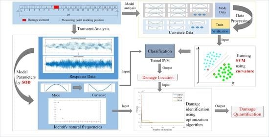
Following the idea of two-stage damage identification, this study investigated the damage identification of beam structures. Based on the analysis of the mapping relationship between the damage location and modal curvature of the beam structure, a support vector machine (SVM) is trained to locate the damage. Compared with other data-driven machine learning methods, the support vector machine can use a limited number of samples to achieve the best generalization effect [21]; it is also favored by a large number of scholars. At the same time, studies [21,22,23,24] have shown that the SVM performs well in damage locations, but it is difficult to quantify damage. The swarm intelligence optimization algorithm can solve this problem well when it is used to identify the degree of damage. Considering the damage degree as an unknown quantity, this study uses the particle swarm optimization (PSO), moth-flame algorithm (MFO), and mayfly algorithm (MA) to calculate the damage degree. Through a large number of simulations and analyses, it is verified that the intelligent optimization algorithm can calculate the damage degree quickly and effectively. To further study the robustness of the method, four levels of noise are set for comparative analysis: no noise, 0.2% noise, 0.5% noise, and 1% noise. The uncertainty of the damage degree identification under different noise levels is analyzed using the Monte-Carlo method.

The remainder of this paper is organized as follows. The second section introduces the principle of the smooth orthogonal decomposition (SOD) and the SVM and the calculation method of normalized curvature. In Section 3, the three swarm intelligent optimization algorithms are introduced in combination with the damage quantification problem, and the fitness function used in this study is proposed. In Section 4, numerical examples of simply supported beams with different damage scenarios are used to verify the proposed method. In Section 5, an uncertainty analysis of the damage degree identification of swarm intelligence algorithms is carried out using the Monte-Carlo method. Finally, this study provides a summary in Section 6.

2. Damage Location

Damage identification is a typical inverse mathematical problem. The two-stage damage identification method divides the damage identification problem into two parts: damage location and damage quantification. Determining the location of damage is the first step. Only when the location of the damage is clear can the damage degree of the damaged part of the structure be identified, and the structure can be better warned, maintained, or replaced. In this study, using the SOD method, the observable response data are transformed into the frequency and mode shape information determined by the structural characteristics we are concerned about, and the modal curvature is obtained. After normalization, it is used as the input of the SVM model to predict the damage location.

2.1. Smooth Orthogonal Decomposition (SOD)

In the field of vibration engineering, the SOD is suitable for identifying lightly damped vibration systems with multiple degrees of freedom [25]. Compared to the proper orthogonal decomposition (POD) method, the SOD method does not require a uniform distribution of the structural mass and can directly identify natural frequencies.

Let the matrix $\mathit{X}$ denote an $n\times N$ ensemble of displacements obtained from $N$ sampling time points from $n$ sensors. The speed dataset can be represented by $\mathit{V}=\dot{\mathit{X}}$. The displacement covariance matrix and velocity covariance matrix can then be expressed as

$${\mathit{R}}_{\mathit{X}\mathit{X}}=\frac{\mathit{X}{\mathit{X}}^T}{N-1},\hspace{1em}{\mathit{R}}_{\mathit{V}\mathit{V}}=\frac{\mathit{V}{\mathit{V}}^T}{N-1}$$

(1)

The SOD can extract mode shapes and natural frequencies from the following generalized eigenvalue problems:

$$\lambda {\mathit{R}}_{\mathit{X}\mathit{X}}\psi ={\mathit{R}}_{\mathit{V}\mathit{V}}\psi ,$$

(2)

where the generalized eigenvalue $\lambda$ is the smooth orthogonal value, and the generalized eigenvector $\psi$ represents the smooth orthogonal mode corresponding to $\lambda$. The generalized eigenvalue problem defined in Equation (2) can be expressed in the matrix form as follows:

$${\mathit{R}}_{\mathit{X}\mathit{X}}\mathit{\Psi }\mathit{\Lambda }={\mathit{R}}_{\mathit{V}\mathit{V}}\mathit{\Psi },$$

(3)

where $\mathit{\Lambda }=diag\left[{\lambda }_1,{\lambda }_2,\cdots ,{\lambda }_n\right]$ and $\mathit{\Psi }=\left[{\psi }_1,{\psi }_2,\cdots ,{\psi }_n\right]$. As the sampling frequency increases, ${\lambda }_i$ approaches the square of the natural frequency ${\omega }_i$, that is, ${\lambda }_i={\omega }_i^2,i=1,2,\cdots ,n$. The system modal matrix $\mathit{\Phi }$ is the inverse transpose of the smooth orthogonal modal matrix $\mathit{\Psi }$, that is, $\mathit{\Phi }={\mathit{\Psi }}^{-T}$.

According to the modal superposition principle, we know that

$$\mathit{X}=\mathit{\Phi }\mathit{Q}, \mathit{V}=\mathit{\Phi }\dot{\mathit{Q}},$$

(4)

where $\mathit{Q}$ denotes the ensemble data of the modal coordinate responses. The covariance matrices in Equation (1) are congruent matrices of the covariance matrices of the modal coordinate responses, as follows:

$${\mathit{R}}_{\mathit{X}\mathit{X}}=\frac{\mathit{\Phi }\mathit{Q}{\mathit{Q}}^T{\mathit{\Phi }}^T}{N-1}=\mathit{\Phi }{\mathit{R}}_{\mathit{Q}\mathit{Q}}{\mathit{\Phi }}^T, {\mathit{R}}_{\mathit{V}\mathit{V}}=\frac{\mathit{\Phi }\dot{\mathit{Q}}{\dot{\mathit{Q}}}^T{\mathit{\Phi }}^T}{N-1}=\mathit{\Phi }{\mathit{R}}_{\dot{\mathit{Q}}\dot{\mathit{Q}}}{\mathit{\Phi }}^T,$$

(5)

where ${\mathit{R}}_{\mathit{Q}\mathit{Q}}=\frac{\mathit{Q}{\mathit{Q}}^T}{N - 1}$ and ${\mathit{R}}_{\dot{\mathit{Q}}\dot{\mathit{Q}}}=\frac{\dot{\mathit{Q}}{\dot{\mathit{Q}}}^T}{N - 1}$.

For undamped free vibration systems, the covariance matrices of the modal coordinate responses are diagonal. Solving the generalized eigenvalue decomposition of Equation (3) is equivalent to the eigenvalue decomposition of the ${\mathit{R}}_{\mathit{X}\mathit{X}}^{-1}{\mathit{R}}_{\mathit{V}\mathit{V}}$. By introducing Equation (5), we obtain

$${\mathit{R}}_{\mathit{X}\mathit{X}}^{-1}{\mathit{R}}_{\mathit{V}\mathit{V}}={\mathit{\Phi }}^{-T}{\mathit{R}}_{\mathit{Q}\mathit{Q}}^{-1}{\mathit{R}}_{\dot{\mathit{Q}}\dot{\mathit{Q}}}{\mathit{\Phi }}^T=\mathit{\Psi }\mathit{\Lambda }{\mathit{\Psi }}^{-1}$$

(6)

Using the transpose and symmetry of matrices, Hu et al. improved Equation (6) and proposed the following new expression [26]:

$${\mathit{R}}_{\mathit{V}\mathit{V}}{\mathit{R}}_{\mathit{X}\mathit{X}}^{-1}=\mathit{\Phi }{\mathit{R}}_{\dot{\mathit{Q}}\dot{\mathit{Q}}}{\mathit{R}}_{\mathit{Q}\mathit{Q}}^{-1}{\mathit{\Phi }}^{-1}=\tilde{\mathit{\Phi }}\mathit{\Lambda }{\tilde{\mathit{\Phi }}}^{-1}$$

(7)

Thus far, the estimated modal matrix $\tilde{\mathit{\Phi }}$ can be directly obtained by the eigenvalue decomposition of the ${\mathit{R}}_{\mathit{V}\mathit{V}}{\mathit{R}}_{\mathit{X}\mathit{X}}^{-1}$. The obtained mode shape vectors are normalized to ensure that their lengths are equal to one.

In practical applications, only low-order modes can be excited with a sufficient energy. Thus, we cannot identify all mode shape vectors completely. It is also very important to determine the order $\widehat{n}$ of the identifiable mode shapes. Take the diagonal elements of ${\mathit{R}}_{\mathit{q}\mathit{q}}={\mathit{\Phi }}^{-1}{\mathit{R}}_{\mathit{X}\mathit{X}}{\mathit{\Phi }}^{-T}$ and arrange them in descending order $\widehat{\lambda }=\left[{\widehat{\lambda }}_1,{\widehat{\lambda }}_2,\cdots ,{\widehat{\lambda }}_{\widehat{n}},{\widehat{\lambda }}_{\widehat{n}+1},\cdots {\widehat{\lambda }}_n\right]$. Because the order of magnitude of the noise eigenvalue is much smaller than the modal eigenvalue, when ${\widehat{\lambda }}_{\widehat{n}}\gg {\widehat{\lambda }}_{\widehat{n}+1}$, we believe that the order of the exact modal shape is $\widehat{n}$ [20]. In this paper, when $\frac{{\widehat{\lambda }}_{\widehat{n}}}{{\widehat{\lambda }}_{\widehat{n}+1}}>10$, we consider ${\widehat{\lambda }}_{\widehat{n}}\gg {\widehat{\lambda }}_{\widehat{n}+1}$.

2.2. Modal Curvature

The curvature ${\phi }^{″}$ is the second derivative of a curve [27]:

$${\phi }^{″}=d^{2}y/d{x}^2$$

(8)

where $y$ is the displacement mode shape function and $x$ is the position coordinate.

When the measuring points are arranged at equal intervals, each element ${\phi }_{ij}^{″}$ in the modal curvature matrix ${\mathit{\Phi }}^{″}$ can be expressed as [27]:

$${\phi }_{ij}^{″}=\frac{y_{i\left(j-1\right)}-2y_{ij}+y_{i\left(j+1\right)}}{h^2}$$

(9)

where $y_{ij}$ represents the modal displacement of the j-th measuring point for the i-th mode, and h represents the distance between the measuring points. Because the measuring points are arranged at equal intervals, the nominal curvature of all modes is multiplied by the $h^2$:

$${\phi }_{ij}^{″}=y_{i\left(j-1\right)}-2y_{ij}+y_{i\left(j+1\right)}$$

(10)

Simultaneously, analogous to the normalization of the mode shape vectors, the modal curvature is also normalized. We call this process normalizing, which ensures that the required modal curvature characteristics are guaranteed to be of the same order of magnitude.

The modal curvature components of the first and last measuring points cannot be calculated using Equation (10) and can be estimated by the following equation (assuming there are $n$ measuring points):

$$\{\begin{array}{c}{\phi }_{11}^{″}=2{\phi }_{12}^{″}-{\phi }_{13}^{″}\\ {\phi }_{1n}^{″}=2{\phi }_{1\left(n-1\right)}^{″}-{\phi }_{1\left(n-2\right)}^{″}\end{array}$$

(11)

2.3. Support Vector Machine (SVM)

The SVM is a generalized linear classifier that classifies the labeled training sample dataset. Its learning strategy is to solve the hyperplane of the optimal (maximized) margin (the minimum distance between the hyperplane and any point of the sample) of the training sample and binary classification of the training dataset [28,29]. A conceptual example of an SVM is shown in Figure 1. However, it is unrealistic to expect only two damage categories for damage locations in practical engineering applications. The damage location problem is a typical multi-classification problem. When an SVM is applied to multi-classification problems, it can be considered as a series of binary classification problems, and the corresponding multi-step binary classification machines should be established.

Suppose we have a training dataset of damaged structures that has only two damage categories:

$$Dataset=\left[\mathit{X};\mathit{Y}\right],$$

(12)

where $\mathit{X}=\left[{\mathit{x}}_1,{\mathit{x}}_2,\cdots ,{\mathit{x}}_n\right]\in {ℝ}^n$ is the set of damage characteristic vectors and $\mathit{Y}=\left[y_1,y_2,\cdots ,y_n\right]$ ($y_i\in \left\{1,-1\right\}$) is the label corresponding to the damage eigenvector. ${\mathit{x}}_{\mathit{i}}$ represents the vector under the i-th damage condition, which refers to the normalized curvature under the i-th damage condition. The hyperplane can be defined as:

$$H\left(\mathit{x}\right)=\mathit{w}\mathit{x}+b=0$$

(13)

where $\mathit{w}$ is the normal vector that controls the normal direction of the hyperplane and $b$ controls the marginal size. The ${\mathit{x}}_{\mathit{i}}$ category can be judged using a hyperplane. If $H\left(\mathit{x}\right)>0$, it is determined that it belongs to damage category I. Conversely, if $H\left(\mathit{x}\right)<0$, it is determined that it belongs to damage category II. The binary classification can be expressed as the following discriminant:

$$\widehat{y}=\mathit{sgn}(\left(\mathit{w}\cdot \mathit{x}\right)+b)$$

(14)

where $\mathit{sgn}(•)$ is the sign discriminant function. If $\left(\mathit{w}\cdot \mathit{x}\right)+b>0$, then $\widehat{y}=1$; if $\left(\mathit{w}\cdot \mathit{x}\right)+b<0$, then $\widehat{y}=-1$.

When $\mathit{w}$ is determined, adjusting $b$ can cause some sample points of damage conditions to fall on $\mathit{w}\mathit{x}+b=1$ and $\mathit{w}\mathit{x}+b=-1$. These characteristic vectors are called the support vectors. The functional margin from the sample point ${\mathit{x}}_{\mathit{i}}$ to the hyperplane under any damage condition can be defined as follows:

$$d_i={\widehat{y}}_{i}H\left({\mathit{x}}_{\mathit{i}}\right)=\left|\mathit{w}{\mathit{x}}_{\mathit{i}}+b\right|$$

(15)

There is significant uncertainty in the function margin. If the parameters $\mathit{w}$ and $b$ are synchronously magnified, the hyperplane will not change, but the function margin $d_i$ will be magnified. Therefore, it is necessary to normalize $\mathit{w}$ and $b$ to obtain the geometric margin:

$$\tilde{d}=\frac{\left|\mathit{w}{\mathit{x}}_{\mathit{i}}+b\right|}{\Vert \mathit{w}\Vert }$$

(16)

The geometric margin that passes through the plane of the two support vectors and is consistent with the normal direction of the optimal hyperplane, that is, the geometric interval between $\mathit{w}\mathit{x}+b=1$ and $\mathit{w}\mathit{x}+b=-1$, can be expressed as:

$$D=2\frac{\left|\mathit{w}{\mathit{x}}_{\mathit{i}}+b\right|}{\Vert \mathit{w}\Vert }=\frac{2}{\Vert \mathit{w}\Vert }$$

(17)

The hyperplane for solving the optimal (maximized) margin of the training sample can be transformed into the following equivalent convex quadratic problem:

$$\begin{gathered} \underset{w,b}{min}\frac{1}{2}{\Vert \mathit{w}\Vert }^2, \\ s.t.\hspace{1em}{y}_i\left(\mathit{w}{\mathit{x}}_{\mathit{i}}+b\right)\ge 1,\hspace{1em}i=1,2,\cdots ,n \end{gathered}$$

(18)

The Lagrange function is introduced to solve Equation (18):

$$L\left(\mathit{w},b,\mathit{\alpha }\right)=\frac{1}{2}{\Vert \mathit{w}\Vert }^2-{\displaystyle \sum }_{i=1}^n{\alpha }_i\left(y_i\left(\mathit{w}{\mathit{x}}_i+b\right)-1\right)$$

(19)

where $\mathit{\alpha }={\left({\alpha }_1,{\alpha }_2,\cdots ,{\alpha }_n\right)}^T$ denotes the Lagrange multiplier vector. According to the Karush–Kuhn–Tucker condition for the differentiable convex problem, the dual problem of Equation (19) can be obtained as [30]:

$$\begin{array}{c}\underset{\alpha }{ma\mathit{x}}\left\{{\displaystyle {\displaystyle \sum }_{i=1}^n}{\alpha }_i-\frac{1}{2}{\displaystyle {\displaystyle \sum }_{i=1}^n}{\displaystyle {\displaystyle \sum }_{j=1}^n}{y}_i{y}_j{\alpha }_i{\alpha }_j{\mathit{x}}_i^T{\mathit{x}}_j\right\}\\ s.t.{\displaystyle {\displaystyle \sum }_{i=1}^n}{\alpha }_i{y}_i=0; {\alpha }_i\ge 0;\hspace{1em}i=1,2,\cdots ,n\end{array}$$

(20)

Assuming that the optimal solution determined by Equation (20) is ${\mathit{\alpha }}^{*}={\left[{\alpha }_1^{*},{\alpha }_2^{*},\cdots ,{\alpha }_n^{*}\right]}^T$, the two parameters that control the hyperplane can be determined by:

$$\begin{array}{c}{\mathit{w}}^{*}={\displaystyle {\displaystyle \sum }_{i=1}^n}{\alpha }_i^{*}{y}_i{\mathit{x}}_{\mathit{i}}\\ b^{*}=\frac{1}{\left|M\right|}{\displaystyle {\displaystyle \sum }_{m\in M}}\left[y_m-{\mathit{w}}^{*}{\mathit{x}}_m\right]\end{array}$$

(21)

where $M$ is the index set of all support vectors and $\left|M\right|$ denotes the cardinality of the set $M$.

However, in practical engineering applications, the data are usually linearly indivisible. In this case, the kernel SVM is constructed using a nonlinear mapping function:

$$\widehat{y}=\mathit{w}\mathit{F}\left(\mathit{x}\right)+b$$

(22)

where $\mathit{F}\left(\mathit{x}\right)$ is a nonlinear mapping function. Similarly, it can be transformed into a convex quadratic problem:

$$\begin{array}{c}\underset{w,b}{min}\frac{1}{2}{\Vert \mathit{w}\Vert }^2\\ s.t. y_i\left(\mathit{w}\mathit{F}\left({\mathit{x}}_{\mathit{i}}\right)+b\right)\ge 1, i=1,2,\cdots ,n\end{array}$$

(23)

The dual problem of Equation (23), similar to Equation (20), can also be constructed as follows:

$$\begin{array}{c}\underset{\alpha }{ma\mathit{x}}\left\{{\displaystyle {\displaystyle \sum }_{i=1}^n}{\alpha }_i-\frac{1}{2}{\displaystyle {\displaystyle \sum }_{i=1}^n}{\displaystyle {\displaystyle \sum }_{j=1}^n}{y}_i{y}_j{\alpha }_i{\alpha }_j{\left(\mathit{F}\left({\mathit{x}}_i\right)\right)}^T\mathit{F}\left({\mathit{x}}_j\right)\right\}\\ s.t. {\displaystyle {\displaystyle \sum }_{i=1}^n}{\alpha }_i{y}_i=0; {\alpha }_i\ge 0; i=1,2,\cdots ,n\end{array}$$

(24)

If the kernel function is defined as $\mathit{k}\left(\mathit{p},\mathit{q}\right)={\left(\mathit{F}\left(\mathit{p}\right)\right)}^T\mathit{F}\left(\mathit{q}\right)$, then Equation (24) can be expressed as:

$$\begin{array}{c}\underset{\alpha }{max}\left\{{\displaystyle {\displaystyle \sum }_{i=1}^n}{\alpha }_i-\frac{1}{2}{\displaystyle {\displaystyle \sum }_{i=1}^n}{\displaystyle {\displaystyle \sum }_{j=1}^n}{y}_i{y}_j{\alpha }_i{\alpha }_{j}k\left(x_i,x_j\right)\right\}\\ s.t. {\displaystyle {\displaystyle \sum }_{i=1}^n}{\alpha }_i{y}_i=0; {\alpha }_i\ge 0; i=1,2,\cdots ,n\end{array}$$

(25)

For the real Euclidean space, the Mercer condition guarantees the arbitrariness of the kernel function $\mathit{k}\left(\mathit{p},\mathit{q}\right)$ [31]. In this manner, we map the linearly indivisible data from the low-dimensional feature space to the high-dimensional feature space. In a high-dimensional space, the original nonlinear separable data will become linearly separable. In this study, because the data are linearly separable, we use the simplest linear kernel function, whose expression is:

$$\mathit{k}\left({\mathit{x}}_i,{\mathit{x}}_j\right)={\mathit{x}}_i^{\mathit{T}}{\mathit{x}}_j$$

(26)

By substituting Equation (26) into Equation (25), we find that it is the same as in Equation (20). Therefore, these two parameters are obtained from Equation (21).

3. Damage Quantification

To obtain accurate damage information, a structure must be finely divided into small elements. It is feasible to consider all of the elements of the entire structure as possible damage elements to establish a structural damage calculation model. However, the problem dimension will increase with an increase in the number of structural elements, and the calculation of swarm optimization algorithms will be extremely complex. In view of the sparseness of the initial damage of the structure, damage localization and damage quantification are considered separately in our work. On the basis that the localization information has been determined, we perform the damage quantitative analysis for the determined damage elements to overcome the curse of dimensionality. However, if the damage localization information is unknown, the search results obtained by swarm optimization algorithms can easily fall into a local optimum.

3.1. Swarm Intelligence Optimization Algorithm

It is difficult to determine an optimal solution for many practical problems. In particular, problems classified as NP-hard cannot be solved using classical optimization methods in a limited amount of time [32]. To determine the damage degree of the structure, an absolute exact solution exists, but cannot be solved analytically. The approximate solution is particularly important for the evaluation of the structural state. To quantify damage when the damage location is known, we use three swarm optimization algorithms to calculate the damage degree. These algorithms include the PSO, MFO, and MA. The convergence trend and calculation error of these three swarm optimization algorithms are compared in this study.

3.1.1. PSO

The PSO is a swarm intelligence optimization algorithm that simulates bird foraging. The solution to the problem is expressed by the position of the particle in the space. The update of the position and state of each particle is related to the social experiences of the particle groups. Based on the information sharing between particles, it can update itself without complex derivative calculations. At the same time, the PSO is not sensitive to the nature of the objective function and can easily jump out of the local optimal value [33], which can be applied to various random fitness functions. When the PSO is applied to quantify the damage, the damage degree of the damaged element is characterized by the position coordinates of each particle. The degree of damage of the damage element is calculated by updating the position state of the particles in the solution space. The pseudo code for the damage degree identification based on the PSO is shown in Algorithm 1.

Algorithm 1: Pseudo code of damage degree identification based on the PSO

Initialize particle swarm position $x_i$ and velocities $v_i \left(i=1, 2, \cdots , N\right)$ Calculate the overall stiffness matrix Calculate fitness function Evaluate fitness results Find personal best $pbest$ and global best $gbest$ Do while stopping criteria are not met     Update velocities and position of particle swarm     Calculate the overall stiffness matrix     Calculate fitness function     Evaluate fitness results     Update $pbest$ and $gbest$ End while Postprocess results and visualization.

3.1.2. MFO

The MFO is a population intelligent optimization algorithm proposed by Australian scholar Mirjalili in 2015 [34]. This is a natural heuristic algorithm that simulates the moth using a lateral orientation to find the light source at night. The moths are actually individuals moving in the search space, and the flames are the best positions that the corresponding moths can reach. Each moth is surrounded by a flame. Once a better solution is obtained, it is updated to the position of the flame in the next generation. Therefore, the moths will never lose their best solutions [35]. At the same time, an adaptive mechanism is proposed to reduce the number of flames adaptively with an increase in iteration times, so that the algorithm can converge better and faster. Compared with other algorithms, the MFO algorithm has the advantages of a simple structure, easy implementation, and fewer parameters [36]. When the MFO is applied to the damage degree optimization model, the damage degree of the damage element is characterized by the position coordinates of the moths. The damage degree of the damage element is calculated by updating the position state of the moths rotating around the flames in the solution space. The pseudo code for the damage degree identification based on the MFO is shown in Algorithm 2.

Algorithm 2: Pseudo code of damage degree identification based on the MFO

Initialize moth position $x_i$ and flame position $y_i \left(i=1,2,\cdots ,N\right)$ Calculate the overall stiffness matrix Calculate moth and flame fitness function Evaluate moth and flame fitness results Establish the corresponding relationship between moth and flame according to fitness value Do while stopping criteria are not met     Update moth position according to flame position     Calculate the overall stiffness matrix     Calculate moth fitness function     Evaluate moth fitness results     Reduce the number of flames     Evaluate flame and moth fitness values     Update flame position and flame fitness     Establish the corresponding relationship between moth and flame according to fitness value End while Postprocess results and visualization.

3.1.3. MA

The MA is a population intelligent optimization algorithm proposed by Zervoudakis and Tsafarakis in 2020 [37], which simulates the flight courtship behavior and mating process of mayflies. The mayflies are divided into males and females. They can update the position of the mayflies and solve the problem by a series of social behaviors (flying, mating, bearing, and replacing). In the process of courtship flight, the male and female mayflies exhibit different social behaviors, but their behaviors depend on the social experience of individuals and groups. This algorithm can be regarded as an improvement of the PSO, which combines the advantages of the PSO, GA, and firefly algorithm (FA). When the MA is applied to the damage degree optimization model, the damage degree of the damage element is represented by the position coordinates of the mayflies. The damage degree of the damage element is calculated by updating the position states caused by a series of social behaviors of the mayflies in the solution space. The pseudo code for the damage degree identification based on the MA is shown in Algorithm 3.

Algorithm 3: Pseudo code of damage degree identification based on the MA

Initialize the male mayfly population $x_i\left(i=1, 2, \cdots ,N\right)$ and velocities $v_i^m\left(i=1, 2,\cdots ,N\right)$ Initialize the female mayfly population $y_j\left(j=1, 2,\cdots ,M\right)$ and velocities $v_j^f\left(j=1, 2,\cdots ,M\right)$ Calculate the overall stiffness matrix Calculate fitness function Evaluate fitness results Find personal best $pbest$ and global best $gbest$ Do while stopping criteria are not met     Update velocities and solutions of males and females     Calculate the overall stiffness matrix     Calculate fitness function     Evaluate fitness results     Rank the mayflies     Mate the mayflies     Calculate the overall stiffness matrix according to offspring     Calculate fitness function     Evaluate fitness results     Evaluate offspring     Separate offspring into male and female randomly     Replace worst solutions with the best new ones     Update $pbest$ and $gbest$ End while Postprocess results and visualization.

3.2. Fitness Function

The traditional fitness function is usually the sum of the residual square of the natural frequency calculated by optimization algorithms and the identified natural frequency. The following fitness functions were used in References [20,38]:

$$Fitness={\displaystyle \sum }_i^n{\left({\omega }_i^r-{\omega }_i^t\right)}^2/{\left({\omega }_i^r\right)}^2$$

(27)

where ${\omega }_i^r$ is the calculated value of the i-th order frequency obtained in each iteration of the optimization algorithms, ${\omega }_i^t$ is the identified i-th order natural frequency value of the structure, and $n$ is the order of the modes involved in the calculation. The calculated natural frequencies of each order are as close to the natural frequencies of each order of the structure as possible during the optimization process. As the objective of optimization, the identified natural frequencies of each order of the structure must be very accurate to ensure calculation accuracy under the fitness function. However, the energy of each mode excited by a structure is typically different. Generally, the energy of the low-order mode is higher and that of the high-order mode is lower, which may affect the accuracy of the SOD method in identifying the modal parameters of each order. To reduce the error caused by the parameters of the identified low-energy mode participating in the calculation, the weighting coefficient ${\alpha }_i$ is added to the traditional fitness function. However, the frequencies of each order usually differ greatly in value, and the denominator in the fitness function is small for low-order frequencies. When the residual values of the calculated natural frequencies and the identified modal frequencies of each order are the same, the low-order frequencies are not stable compared with the high-order frequencies. To mitigate this effect, the fitness function is obtained by adding the weighting coefficient ${\beta }_i$ to the fitness function. The fitness function is given by:

$$Fitness={\displaystyle \sum }_i^{\widehat{n}}\left({\alpha }_i\ast {\beta }_i\ast {\left({\omega }_i^r-{\omega }_i^c\right)}^2/{\left({\omega }_i^r\right)}^2\right)$$

(28)

where ${\omega }_i^c$ is the natural frequency of the structure extracted by the SOD method; ${\alpha }_i=\frac{{\widehat{\lambda }}_i}{{{\displaystyle \sum }}_{i=1}^{\widehat{n}}{\widehat{\lambda }}_i}$, and ${\beta }_i=\frac{{\omega }_i^c}{{{\displaystyle \sum }}_{i=1}^{\widehat{n}}{\omega }_i^c}$, where the values of $\widehat{n}$ and ${\widehat{\lambda }}_i$ are the same as those in Equation (7).

3.3. Damage Identification Steps

The frequencies obtained by the SOD method are used to compute the fitness function of the swarm optimization algorithms. The damage location method based on the SOD-SVM is used to identify the damage elements of the beam structure, and the number of identified damage elements is taken as the dimension of the solution space in the swarm optimization algorithms. Compared with directly considering the stiffness of all structural elements as the unknown quantity of the intelligent algorithms, the two-stage method significantly reduces the number of unknown quantities. Therefore, it is conducive to accelerating the convergence speed of the algorithms and improving the optimization accuracy. The damage identification algorithm is shown in Figure 2.

4. Numerical Example

The beam structure is divided into 20 elements, and the model is established and simulated using finite element analysis software. The beam model is shown in Figure 3. The span of the simply supported beam is $2.0 \mathrm{m}$ and the section size is $0.1 \mathrm{m}\times 0.02 \mathrm{m}$, the Young’s Modulus is $E=210 \mathrm{GPa}$, the density is $\rho =7850 \mathrm{kg}/{\mathrm{m}}^3$, and the Poisson’s ratio is $\gamma =0.3$.

The local damage of this simply supported beam is simulated by reducing the elastic modulus of a specific element [20], as follows:

$$E_i^d=\left(1-d_i\right)E$$

(29)

where $E_i^d$ represents the elastic modulus of the i-th damaged element, and $d_i$ represents the percentage of stiffness reduction of the i-th element (represented as the degree of damage in this study). Gaussian white noise is used as random excitation, and the transient dynamic analysis of the model is carried out to obtain the displacement and velocity response data of each node. At the same time, in order to study the noise robustness of the proposed damage identification method, 0.2%, 0.5%, and 1% noise are added to the extracted displacement and velocity response data, respectively. The signal is contaminated by white noise in terms of:

$$noise=n_{level}\times normrnd\left(0, \sigma , \left[s_{size}\right]\right)$$

(30)

$$X_n=X+noise$$

(31)

where $n_{level}=0.2\%, 0.5\%, \mathrm{or} 1\%$ indicates the noise level, $\sigma$ is the covariance of the original signal, $S_{size}$ is sequence length of the original signal, $normrnd(•)$ is a subroutine to generate normal distribution random numbers, X represents the original signal, and $X_n$ indicates the signal polluted by white noise.

4.1. Single Damage Condition

The damage degree of each element of the established simply supported beam from 1% to 90% (increasing by 1%) is simulated separately, the first-order mode of each damage model is extracted, and the modal curvature is calculated. Through the above operations, we obtain $20\times 90=1800$ groups of data. Another 90 groups of data calculated for the undamaged beam are added to the dataset, and a total of 1890 groups of data are used as the dataset. Using a 75–25 split, the training and verification sets contained 1417 and 473 groups of data, respectively. The SVM model is trained using these data. The damage location of the above datasets is identified using the SVM. The results show that the recognition accuracy of the damage location of the training and verification sets reaches 100%. It can be seen that the SVM can make a good judgment on the location of a single point of damage in the simulated cases.

To further determine the accuracy and robustness of the SVM model, 10%, 15%, 20%, and 25% damage is preset for each element of the simply supported beam. White noise excitation is used to excite the damage model for transient dynamic analysis, and the displacement and velocity response data are obtained. White noise with different degrees is added to the responses (the noise levels are 0.2%, 0.5%, or 1%). The mode shapes and natural frequencies of the structure are extracted using the SOD. As shown in Figure 4, for the eighth element with 20% damage, under the influence of 0.5% noise degree, we can determine and extract the modal parameters of the $\widehat{n}=3$ mode order. The frequencies identified by the SOD and those extracted using ANSYS are compared in

Table 1. Frequency calculation value of the SOD and ANSYS extracted value (single damage condition).

Damage Condition	Frequency Order	Ansys	Noise Level	SOD	Error
Element 8 takes 20% damage	1	57.945	Without	57.954	0.015%
			0.2%	57.924	0.037%
			0.5%	57.901	0.077%
			1%	57.870	0.130%
	2	231.92	Without	231.913	0.003%
			0.2%	231.874	0.020%
			0.5%	231.942	0.010%
			1%	232.173	0.109%
	3	520.72	Without	521.216	0.095%
			0.2%	520.983	0.050%
			0.5%	520.942	0.043%
			1%	520.439	0.054%

. The results show that under different noise levels, the differences between the first three frequency identification values and the extracted values are within 0.15%, indicating that the SOD method can accurately identify the frequencies of a single damaged simply supported beam.

The modal energies of each excitation order are often different. To accurately evaluate the performance of the established SVM model, the test set is composed of the identified modal shape curvatures with the largest modal energy, which is the first-order modal parameter obtained by the SOD method. The statistical verification results for the test set are shown in Figure 5. The results show that the localization accuracy of the SVM for the damage location increases with an increase in the damage degree. The more serious the damage, the easier it is to detect. When the damage is 10% and the noise level reaches 1%, the accuracy of the SVM model is more than 85%. When the noise level is reduced to 0.5%, the recognition accuracy reaches 97.56%, which is significantly improved. When the noise level drops to 0.2%, the position recognition accuracy reaches 100%, even if the local damage is 10%. When the degree of damage reaches 15%, the accuracy is still above 95%, even in the case of high-level noise. At the same time, when the damage degree reaches 20%, even under the influence of 0.5% noise, the localization accuracy reaches 100%. The statistical results show that the damage location method based on the SOD-SVM can effectively identify the damage location under a single damage condition. After the location of the damage element is determined, the subsequent damage degree optimization model is reduced to a one-dimensional search problem.

The eighth element is chosen as the damaged element to illustrate the performance of the searching algorithm. After the SVM determines that the damage element is the eighth element, the stiffness loss ratio of the eighth element is set as an unknown parameter and the first three frequencies are substituted into the fitness function. The search range of the stiffness loss ratio of the element is set to [0, 1]. The fitness evolution of the three swarm intelligent optimization algorithms with an increase in the iteration number is shown in Figure 6. It can be observed that after the dimension is reduced, all three algorithms can converge quickly. The results of the stiffness loss ratio of the damaged element calculated by the three algorithms under different noise levels are listed in

Table 2. Element stiffness reduction ratio (single damage condition).

Damage Condition	Noise Level	Algorithm	Calculated Value	Error
Element 8 takes 20% damage	Without noise	PSO	19.64%	1.80%
		MFO	19.64%	1.80%
		MA	19.64%	1.80%
	0.2%	PSO	20.51%	2.55%
		MFO	20.51%	2.55%
		MA	20.51%	2.55%
	0.5%	PSO	20.87%	4.35%
		MFO	20.87%	4.35%
		MA	20.87%	4.35%
	1%	PSO	21.74%	8.70%
		MFO	21.74%	8.70%
		MA	21.74%	8.70%

. The results demonstrate that swarm intelligence algorithms have good accuracy in the damage identification of simple supported beams with single damage. It should also be noted that the greater the noise level, the greater the deviation in the predicted damage degree. At a noise level of 1%, the maximum error is 8.70%.

4.2. Multiple Damage Condition

Two-element damage is used to represent multi-element damage. The structural damage of each element of the simply supported beam from 10% to 90% (increased by 10%) is simulated separately, the first-order mode of each damage model is extracted, and the modal curvature is calculated. Through the above operations, we can obtain 15,390 groups of data. Another 81 groups of data for calculated undamaged and 1620 groups of data for single damage of each element are added to the dataset, and a total of 17,091 groups of data are used as the dataset. Using a 75–25 split, the training and verification set had 12,818 and 4273 groups of data, respectively. The SVM model is trained using these data. The damage location of the above datasets is identified using the SVM. The results show that the recognition accuracy of the damage location of the training set is 100%, and that of the verification set is 99.91%. It can be seen that the SVM can also make a good judgment on the location of multiple damages in the simulated cases.

Similarly, 10%, 15%, 20%, and 25% damages are preset for each of the two elements of the simply supported beam. White noise excitation is used to excite the damage model for transient dynamic analysis, and displacement and velocity response data are obtained. White noise with different degrees is added to the responses (the noise levels are 0.2%, 0.5%, or 1%). As shown in Figure 7, for the fifth element with 30% damage and the tenth element with 20% damage, under the influence of 1% noise degree, we can determine and extract the modal parameters of the $\widehat{n}=2$ mode order. The frequencies identified by the SOD and those extracted using ANSYS are compared in

Table 3. Frequency calculation value of the SOD and ANSYS extracted value (multiple damage condition).

Damage Condition	Frequency Order	Ansys	Noise Level	SOD	Error
Element 5 takes 30% damage and element 10 takes 20% damage	1	57.341	Without	57.362	0.036%
			0.2%	57.316	0.044%
			0.5%	57.328	0.023%
			1%	57.284	0.100%
	2	228.67	Without	228.684	0.006%
			0.2%	228.819	0.065%
			0.5%	228.976	0.134%
			1%	228.935	0.116%

. The results show that under different noise levels, the differences between the first three frequency identification values and the extracted values are within 0.15%, which indicates that the SOD method can accurately identify the frequencies of multiple damaged simply supported beams.

Similarly, the test set is composed of the identified modal shape curvatures with the largest modal energy, which is the first-order modal parameter obtained using the SOD method. The statistical verification results for the test set are shown in Figure 8. The results show that the localization accuracy of the SVM for the damage location increases with an increase in the damage degree. The more serious the damage, the easier it is to detect. When the damage is 10% and the noise level reaches 1%, the accuracy of the SVM model is only 60%; however, when the noise level is reduced to 0.5%, the recognition accuracy reaches 93.2%, which is significantly improved. When the noise level drops to 0.2%, the position recognition accuracy reaches 98%, even if the local damage is 10%. When the damage degree reaches 20%, the accuracy is still above 83.2% even in the case of high-level noise. When the damage degree reaches 25%, the accuracy is still above 91.2%, even in the case of high-level noise. At the same time, when the damage degree reaches 20%, even under the influence of 0.5% noise, the localization accuracy reaches 99%. The statistical results show that the damage location method based on the SOD-SVM can effectively identify the damage location under multiple damage conditions. After the location of the damage elements is determined, the subsequent damage degree optimization model is reduced to a two-dimensional search problem.

To illustrate the performance of the search algorithm, the fifth and tenth elements are selected as the damaged elements. After the SVM determines that the damage elements are the fifth and tenth elements, the stiffness loss ratios of the fifth and tenth elements are set as unknown parameters, and the first two frequencies are substituted into the fitness function. The search range of the stiffness loss ratios of the element is set to [0, 1]. The fitness evolution of the three swarm intelligent optimization algorithms with an increase in the iteration number is shown in Figure 9. It can be observed that after the dimension is reduced, all three algorithms can converge quickly. The results of the stiffness loss ratio of the damaged element calculated by the three algorithms under different noise levels are listed in

Table 4. Element stiffness reduction ratio (multiple damage condition).

Damage Condition	Noise Level	Element Number	Algorithm	Calculated Value	Error
Element 5 takes 30% damage and element 10 takes 20% damage	Without noise	5	PSO	29.95%	0.17%
			MFO	29.95%	0.17%
			MA	29.95%	0.17%
		10	PSO	19.53%	2.35%
			MFO	19.53%	2.35%
			MA	19.53%	2.35%
	0.2%	5	PSO	29.25%	2.50%
			MFO	29.25%	2.50%
			MA	29.25%	2.50%
		10	PSO	20.99%	4.95%
			MFO	20.99%	4.95%
			MA	20.99%	4.95%
	0.5%	5	PSO	28.97%	3.43%
			MFO	28.97%	3.43%
			MA	28.97%	3.43%
		10	PSO	21.89%	9.45%
			MFO	21.89%	9.45%
			MA	21.89%	9.45%
	1%	5	PSO	28.63%	4.57%
			MFO	28.63%	4.57%
			MA	28.66%	4.47%
		10	PSO	22.04%	10.20%
			MFO	22.04%	10.20%
			MA	22.03%	10.15%

. The results demonstrate that swarm intelligence algorithms have good accuracy in the damage identification of simple supported beams with single damage. It should also be noted that the greater the noise level, the greater the deviation in the predicted damage degree. At a noise level of 1%, the maximum error is 10.20%.

5. Uncertainty Analysis of Identification Results of Swarm Intelligence Optimization Algorithm

Swarm intelligence algorithms typically result in deviations. Algorithm research usually requires multiple operations. The uncertainty of the results is affected by many factors. To comprehensively evaluate the advantages and disadvantages of the algorithms, the identification results, including the mean, variance, and standard deviation, are analyzed using a statistical method. For the damage degree calculation model, we also need to perform statistics on the calculation results to provide more reliable guidance for structural health assessment.

5.1. Uncertainty Analysis of Single Damage Condition

As shown in Figure 10, 20% damage is preset for the eighth element of the simply supported beam model. The displacement and velocity response data are obtained under random excitations of the structure using the Monte-Carlo method. The response data are polluted by noise at four levels (no noise, 0.2% noise, 0.5% noise, and 1% noise). The natural frequency (including the weight) of each order and damage location are obtained using the SOD-SVM. Then, the searching algorithms (PSO, MFO, and MA) are used for the damage degree calculations. To clearly compare the calculation results of the three intelligent optimization algorithms, the natural frequency order used in the calculation is fixed at 2. The error distributions of the calculation results of these algorithms are shown in Figure 11. It can be observed that the number of outliers of calculation error is very small, but the number of outliers increases with the increase of noise. And the identification error dispersion increases with the level of noise. This illustrates that the prediction uncertainty of the structural damage degree optimization model increases with an increase in measurement noise. However, the prediction errors are low, which suggests that swarm intelligence optimization algorithms can effectively predict the damage degree under single damage conditions after dimensionality reduction.

5.2. Uncertainty Analysis of Multiple Damage Condition

As shown in Figure 12, the fifth element of the simply supported beam model is preset with 30% damage, and the tenth element is preset with nine levels of damage degrees (10%, 20%, 30%, 40%, 50%, 60%, 70%, 80%, and 90%). The displacement and velocity response data are obtained by random excitations of the beams under the abovementioned nine working conditions using the Monte-Carlo method. The response data are polluted by noise at four levels (no noise, 0.2% noise, 0.5% noise, and 1% noise). The natural frequency (including weight) of each order and damage locations are obtained by the SOD-SVM, and the algorithms (PSO, MFO, and MA) are used for multiple calculations. Similarly, the natural frequency order involved in the calculation is fixed at 2. The means and standard deviations of the results calculated using the three algorithms are shown in Figure 13, Figure 14 and Figure 15. The calculated mean values are close to the theoretical damage values, and the standard deviations are relatively small. This suggests that, for the multiple damage condition damage degree optimization model, swarm intelligence optimization algorithms can obtain calculation values with stable values and acceptable uncertainties. At the same time, when the damage degree is relatively small (less than or equal to 40%), the noise will make the calculation result of the group optimization algorithm on the damage degree larger, and the greater the noise is, the smaller the calculation result will be. This is disadvantageous to the calculation of damage degree accuracy, but it is beneficial to the safety maintenance of the structure. The standard deviations of the nine working conditions with increasing damage degrees are counted. It can be seen that the standard deviation shows a descending trend with an increase in the damage value; thus, the calculation uncertainty decreases with an increase in the damage degree.

6. Conclusions

In this study, a two-stage damage identification method for beam structures based on an SVM and swarm intelligence algorithms is studied, and the method is verified by a simple supported beam example. First, the normalized modal curvature is calculated, the mapping relationship between the damage location and modal curvature of the beam structures is established, and the SVM model for the damage location is trained. Based on the pre-trained SVM damage location model, the SOD method is introduced to identify the mode shape of the damaged structure. The modal curvature, which is used as the input data of the SVM model for damage location, is calculated using the second-order central difference of the identified mode shapes. The SOD-SVM damage location method is affected by noise when the degree of damage is low. Nevertheless, at a noise level of 0.5% and below, it can accurately locate the damage, even in the case of small damage. In the second step, the stiffness loss of the damaged element located by the SVM is considered as the optimization objective of the swarm intelligence algorithms. Combined with the frequencies obtained by the SOD method, the three swarm intelligent algorithms (PSO, MFO, and MA) are used to calculate the stiffness loss of the damaged element. The results show that all three swarm intelligence algorithms can converge quickly. Even in the case of strong noise pollution, the deviation in the calculated damage is still small (mean deviation within 3%). The Monte-Carlo method is used to calculate the degree of damage under the influence of different noise levels. It is found that the greater the noise, the more dispersed the calculation of damage degree and the greater the uncertainty; the greater the degree of damage, the more accurate the value of the damage calculation results, and the smaller the uncertainty. In summary, the method proposed in this study can accurately identify damage to beam structures. Even under the influence of noise, this method is reliable. In the future, it is necessary to study the application of this algorithm in the damage identification of complex structures.

References

1. Furinghetti, M.; Pavese, A.; Lunghi, F.; Silvestri, D. Strategies of structural health monitoring for bridges based on cloud computing. J. Civ. Struct. Health Monit. 2019, 9, 607–616. [Google Scholar] [CrossRef]
2. O’Reilly, G.J.; Perrone, D.; Fox, M.; Monteiro, R.; Filiatrault, A.; Lanese, I.; Pavese, A. System Identification and Seismic Assessment Modeling Implications for Italian School Buildings. J. Perform. Constr. Facil. 2019, 33, 04018089. [Google Scholar] [CrossRef]
3. Lin, Y.Q.; Ren, W.X. Stochastic state space model-based damage detection of engineering structures. J. Vib. Eng. 2007, 20, 599–605. [Google Scholar] [CrossRef]
4. Alvandi, A.; Cremona, C. Assessment of vibration-based damage identification techniques. J. Sound Vib. 2006, 292, 179–202. [Google Scholar] [CrossRef]
5. He, J.; Zhou, Y. A novel mode shape reconstruction method for damage diagnosis of cracked beam. Mech. Syst. Signal Process. 2019, 122, 433–447. [Google Scholar] [CrossRef]
6. Pandey, A.; Biswas, M.; Samman, M. Damage detection from changes in curvature mode shapes. J. Sound Vib. 1991, 145, 321–332. [Google Scholar] [CrossRef]
7. Wahab, M.A.; De Roeck, G. Damage detection in bridges using modal curvatures: Application to a real damage scenario. J. Sound Vib. 1999, 226, 217–235. [Google Scholar] [CrossRef]
8. Nguyen, D.H.; Nguyen, Q.B.; Bui-Tien, T.; De Roeck, G.; Wahab, M.A. Damage detection in girder bridges using modal curvatures gapped smoothing method and Convolutional Neural Network: Application to Bo Nghi bridge. Theor. Appl. Fract. Mech. 2020, 109, 102728. [Google Scholar] [CrossRef]
9. Ratcliffe, C. DAMAGE DETECTION USING A MODIFIED LAPLACIAN OPERATOR ON MODE SHAPE DATA. J. Sound Vib. 1997, 204, 505–517. [Google Scholar] [CrossRef]
10. Aydin, K.; Kisi, O. Damage detection in Timoshenko beam structures by multilayer perceptron and radial basis function networks. Neural Comput. Appl. 2012, 24, 583–597. [Google Scholar] [CrossRef]
11. Yang, J.; Zhang, L.; Chen, C.; Li, Y.; Li, R.; Wang, G.; Jiang, S.; Zeng, Z. A hierarchical deep convolutional neural network and gated recurrent unit framework for structural damage detection. Inf. Sci. 2020, 540, 117–130. [Google Scholar] [CrossRef]
12. Li, D.; Wang, Y.; Yan, W.-J.; Ren, W.-X. Acoustic emission wave classification for rail crack monitoring based on synchrosqueezed wavelet transform and multi-branch convolutional neural network. Struct. Health Monit. 2021, 20, 1563–1582. [Google Scholar] [CrossRef]
13. Mehrjoo, M.; Khaji, N.; Ghafory-Ashtiany, M. Application of genetic algorithm in crack detection of beam-like structures using a new cracked Euler–Bernoulli beam element. Appl. Soft Comput. 2012, 13, 867–880. [Google Scholar] [CrossRef]
14. Daei, M.; Mirmohammadi, S.H. A flexibility method for structural damage identification using continuous ant colony optimization. Multidiscip. Model. Mater. Struct. 2015, 11, 186–201. [Google Scholar] [CrossRef]
15. Huang, M.; Lei, Y.; Cheng, S. Damage identification of bridge structure considering temperature variations based on particle swarm optimization-cuckoo search algorithm. Adv. Struct. Eng. 2019, 22, 3262–3276. [Google Scholar] [CrossRef]
16. Kang, F.; Li, J.-J.; Xu, Q. Damage detection based on improved particle swarm optimization using vibration data. Appl. Soft Comput. 2012, 12, 2329–2335. [Google Scholar] [CrossRef]
17. Fernández-Martínez, J.L.; Fernández-Muñiz, Z. The curse of dimensionality in inverse problems. J. Comput. Appl. Math. 2020, 369, 112571. [Google Scholar] [CrossRef]
18. Hinrichs, A.; Prochno, J.; Ullrich, M. The curse of dimensionality for numerical integration on general domains. J. Complex. 2019, 50, 25–42. [Google Scholar] [CrossRef] [Green Version]
19. Debing, Z.; Hui, C.; Weifeng, N. Two-Stage Damage Detection of Beam Structure Based on Improved PSO Algorithm. IOP Conf. Series Earth Environ. Sci. 2021, 634, 012060. [Google Scholar] [CrossRef]
20. Hu, Z.; Zhang, P. Damage Identification of Structures Based on Smooth Orthogonal Decomposition and Improved Beetle Antennae Search Algorithm. Adv. Civ. Eng. 2021, 2021, 8857356. [Google Scholar] [CrossRef]
21. Huang, M.; Cheng, X.; Zhu, Z.; Luo, J.; Gu, J. A Novel Two-Stage Structural Damage Identification Method Based on Superposition of Modal Flexibility Curvature and Whale Optimization Algorithm. Int. J. Struct. Stab. Dyn. 2021, 21, 2150169. [Google Scholar] [CrossRef]
22. Bao, Y.; Song, C.; Wang, W.; Ye, T.; Wang, L.; Yu, L. Damage Detection of Bridge Structure Based on SVM. Math. Probl. Eng. 2013, 2013, 490372. [Google Scholar] [CrossRef] [Green Version]
23. Satpal, S.B.; Guha, A.; Banerjee, S. Damage identification in aluminum beams using support vector machine: Numerical and experimental studies. Struct. Control Health Monit. 2016, 23, 446–457. [Google Scholar] [CrossRef]
24. Seyedpoor, S.M.; Nopour, M.H. A two-step method for damage identification in moment frame connections using support vector machine and differential evolution algorithm. Appl. Soft Comput. 2020, 88, 106008. [Google Scholar] [CrossRef]
25. Hu, Z.-X.; Huang, X.; Wang, Y.; Wang, F. Extended Smooth Orthogonal Decomposition for Modal Analysis. J. Vib. Acoust. 2018, 140, 041008. [Google Scholar] [CrossRef]
26. Hu, Z.; Li, J.; Zhi, L.; Huang, X. Modal Identification of damped vibrating systems by iterative smooth orthogonal decomposition method. Adv. Struct. Eng. 2021, 24, 755–770. [Google Scholar] [CrossRef]
27. Liu, Y.L.; Shi, S.P.; Liao, W. Bridge damage identification using curvature mode shapes. J. Vib. Shock 2011, 30, 77–81+96. [Google Scholar] [CrossRef]
28. Yuan, Y.; Zhang, M.; Luo, P.; Ghassemlooy, Z.; Lang, L.; Wang, D.; Zhang, B.; Han, D. SVM-based detection in visible light communications. Optik 2017, 151, 55–64. [Google Scholar] [CrossRef]
29. Huang, M.; Lei, Y.; Li, X.; Gu, J. Damage Identification of Bridge Structures Considering Temperature Variations-Based SVM and MFO. J. Aerosp. Eng. 2021, 34, 04020113. [Google Scholar] [CrossRef]
30. Zhang, F.; Wang, F.; Zhang, J.; Zuo, T. SVM aided LEDs selection for generalized spatial modulation of indoor VLC systems. Opt. Commun. 2021, 497, 127161. [Google Scholar] [CrossRef]
31. Sebald, D.J.; Bucklew, J.A. Support vector machine techniques for nonlinear equalization. IEEE Trans. Signal Process. 2000, 48, 3217–3226. [Google Scholar] [CrossRef]
32. Knuth, D.E. Postscript about NP-hard problems. ACM SIGACT News 1974, 6, 15–16. [Google Scholar] [CrossRef]
33. Tsafarakis, S.; Marinakis, Y.; Matsatsinis, N. Particle swarm optimization for optimal product line design. Int. J. Res. Mark. 2011, 28, 13–22. [Google Scholar] [CrossRef]
34. Mirjalili, S. Moth-flame optimization algorithm: A novel nature-inspired heuristic paradigm. Knowl. Based Syst. 2015, 89, 228–249. [Google Scholar] [CrossRef]
35. Mohanty, B. Performance analysis of moth flame optimization algorithm for AGC system. Int. J. Model. Simul. 2019, 39, 73–87. [Google Scholar] [CrossRef]
36. Savsani, V.; Tawhid, M.A. Non-dominated sorting moth flame optimization (NS-MFO) for multi-objective problems. Eng. Appl. Artif. Intell. 2017, 63, 20–32. [Google Scholar] [CrossRef]
37. Zervoudakis, K.; Tsafarakis, S. A mayfly optimization algorithm. Comput. Ind. Eng. 2020, 145, 106559. [Google Scholar] [CrossRef]
38. Khatir, S.; Dekemele, K.; Loccufier, M.; Khatir, T.; Wahab, M.A. Crack identification method in beam-like structures using changes in experimentally measured frequencies and Particle Swarm Optimization. Comptes Rendus Mécanique 2018, 346, 110–120. [Google Scholar] [CrossRef]
Figure 1. Conceptual model of SVM.
Buildings 12 01950 g001
Figure 2. Schematic diagram of the damage identification.
Buildings 12 01950 g002
Figure 3. Undamaged simply supported beam model.
Buildings 12 01950 g003
Figure 4. Eigenvalue diagram of R q q for single damaged simple supported beam.
Buildings 12 01950 g004
Figure 5. Single damage location identification.
Buildings 12 01950 g005
Figure 6. Fitness of algorithms under single damage condition. (a) Without noise; (b) 0.2% noise; (c) 0.5% noise; and (d) 1% noise.
Buildings 12 01950 g006
Figure 7. Eigenvalue diagram of R q q for simple supported beam with multiple damage.
Buildings 12 01950 g007
Figure 8. Multiple damage location identification.
Buildings 12 01950 g008
Figure 9. Fitness of algorithms under multiple damage condition. (a) Without noise; (b) 0.2% noise; (c) 0.5% noise; and (d) 1% noise.
Buildings 12 01950 g009aBuildings 12 01950 g009b
Figure 10. Single damage simply supported beam model.
Buildings 12 01950 g010
Figure 11. Damage degree calculation error of single damage condition. (a) Without noise; (b) 0.2% noise; (c) 0.5% noise; and (d) 1% noise.
Buildings 12 01950 g011
Figure 12. Multiple damage simply supported beam model.
Buildings 12 01950 g012
Figure 13. Damage degree calculation value of multiple damage condition based on the PSO. (a) Without noise; (b) 0.2% noise; (c) 0.5% noise; and (d) 1% noise.
Buildings 12 01950 g013aBuildings 12 01950 g013b
Figure 14. Damage degree calculation value of multiple damage condition based on the MFO. (a) Without noise; (b) 0.2% noise; (c) 0.5% noise; and (d) 1% noise.
Buildings 12 01950 g014
Figure 15. Damage degree calculation value of multiple damage condition based on the MA. (a) Without noise; (b) 0.2% noise; (c) 0.5% noise; and (d) 1% noise.
Buildings 12 01950 g015